LARGE SCALE GEODETIC LEAST SQUARES ADJUSTMENT BYDISSECTION AND ORTHOGONAL DECOMPOSITION

Gene H. GolubRobert J. Plemmons

STAN-CS-79-774November 19 7 9

DEPARTMENT OF COMPUTER SCIENCESchool of Humanities and Sciences

STANFORD UNIVERSITY

LARGE SCALE GEODETIC LEAST SQUARES ADJUSTMENT BY

DISSECTION AND ORTHOGONAL DECOMPOSITION

bY

Gene H. Golub*Computer Science Department

Stanford UniversityStanford, CA 94305

**-- Robert J. PlemmonsDepartments of Computer Science and Mathematics

University of TennesseeKnoxville, TN 37916

* Research supported in part by U.S. Army Grant DAAG29-77-GO179 andby National Science Foundation Grant MCS78-11985.

** Research supported in part by U.S. Army Grant D&%29-77-G0166.

ABSTRACT

Very large seal@ matrix problems currently arise in the context

of accurately computing the coordinates of points on the surface of

the earth. Here g.eodesists adjust the approximate values of these

coordinates by computing least squares solutions to large sparse systems

of equations which result from relating the coordinates to certain ob-

servations such as distances or angles between points. The purpose of

this paper is to suggest an alternative to the formation and solution of

the normal eqgations for these least squares adjustment problems. In

particular, it is shown how a block-orthogonal decomposition method can

be used in conjunction with a nested dissection scheme to produce an

algorithm for solving such ,problems which combines efficient data

management with numerical stability. As an indication of the magnitude

that these least squares adjustment problems can sometimes attain, the

forthcoming readjustment of the North American Datum in 1983 by the

National Geodetic Survey is discussed. Here it becomes necessary to

linearize and solve an overdetermined system of approximately ~,OOO,OOO

equations in 400,000 unknowns - a truly large-scale matrix problem.

1. Introduction.

Recent technological advances have made possible the collection of

vast amounts of raw data describing--certain physical phenomena. As a

result, the sheer volume of the data has necessitated the development

of new elaborate schemes for processing and interpreting it in detail.

An example is in the adjustment of geodetic data.

Geodesy is the branch of applied mathematics which is concerned

with the determination of the size and shape of the earth, the directions

of lines and the coordinates of stations or points on the earth's surface.

Applications of this science include mapping and charting, missile and

space operations, earthquake prediction,and navigation. The current use

of electronic distance measuring equipment and one-second theodolites

for angle measurements by almost all surveyors necessitates modern ad-

justment procedures to guard against the possibility of blundersas well as

to obtain a better estimate of the unknown quantities being measured. The

number of observations is always larger than the minimum required to

determine the unknowns. The relationships among the unknown quantities

- and the observations lead to an overdetermined system of nonlinear equations.

The measurements are then usually adjusted in the sense of least squares

by computing the least squares solution to a linearized form of the system

that is not rank deficient.

In general, a geodetical position network is a mathematical model

consisting of several mesh-points or geodetic stations, with unknown posi-

tions over a reference surface or in three-dimensional space. These stations

are normally connected by lines, each representing one or more observations

involving the two stations terminating the line. The observations may be

angles or distances,and thus they lead to nonlinear equations involving,

for example, trigonometric identities and distance formulas relating

the unknown coordinates. Each equation typically involves only a small

number of unknowns.

As an illustration of the sheer magnitude that some of these problems

can attain, we mention the readjustment of the North American Datum -

a network of reference points on the North American continent whose

longitudes, latitudes and, in some cases, altitudes must be known to an

accuracy of a few centimeters. "I'his ten-year project by the U.S. National

Geodetic Survey is expected to be completed by 1983. The readjusted net-

work with very accurate coordinates is necessary to regional planners,

engineers and surveyors, who need accurate reference points to make maps

and s,pecify boundary lines; to navigators; to road builders; and to energy

resource developers and distributors. Very briefly, the problem is to use

some ~,OOO,OOO observations relating the positions of approximately

200,000 stations (400,000 unknowns) in order to readjust the tabulated values

for their latitudes and longitudes. This leads to one of the largest single

computational efforts ever attempted - that of computing a least squares

solution of a very sparse system of ~,OOO,OOO nonlinear equations in

400,000 unknowns. This problem is described in detail by Meissl [1979],

by Avila and Tomlin [1979], and from a layman's point of view by Kolata

[X978] in Science.

In general then, geodetical network adjustment problems can lead

(after linearization) to a very large sparse overdetermined system of m

linear equations in n unknowns

2

t

Ax,--

where the matrix A , called the observation matrix, has f'ull column

rank. The least squares solution to (1.1) is then the unique solution

(1.1)

to the <problem:

mixnilb- AxlIp l

An equivalent formulation of the problem is the following: one seeks to

determine vectors y and r such that r + Ay = b and A% = 0 .

The least squares solution to (1.1) is then the unique solution y to

the nonsingular system of normal equations

AtAy = Atb .

The linear system of equations (1.2) is usually solved by computing

the Choleskv factorization

AtA = RtR , R =

and then solvingt

Rw = Atb by forward substitution and Ry =w by-

back substitution. The upper triangular matrix R is called the

Choleskv factor of A .

(1.2)

Most algorithms for solving geodetic least squares adjustment problems

( see Ashkenazi [1971], Bomford [1971], Meissl [1979] or Avila and Tomlin

[1979])typically involve the formation and solution of some (weighted)

form of the normal equations (1.2). But because of the size of these

problems and the high degree of accuracy desired in the coordinates, it

3

is important that particular attention be paid to sparsity considerations

when forming AtA as well as to the numerical stability of the algorithm

being used. It is generally agreed in modern numerical analysis theory

(see Golub [1965], Lawson and Hanson [lg?+] or Stewart [1978])that ortho-

gonal decomposition methods applied directly to the matrix A in (1.1) are

preferable to the calculation of the normal equations whenever numerical

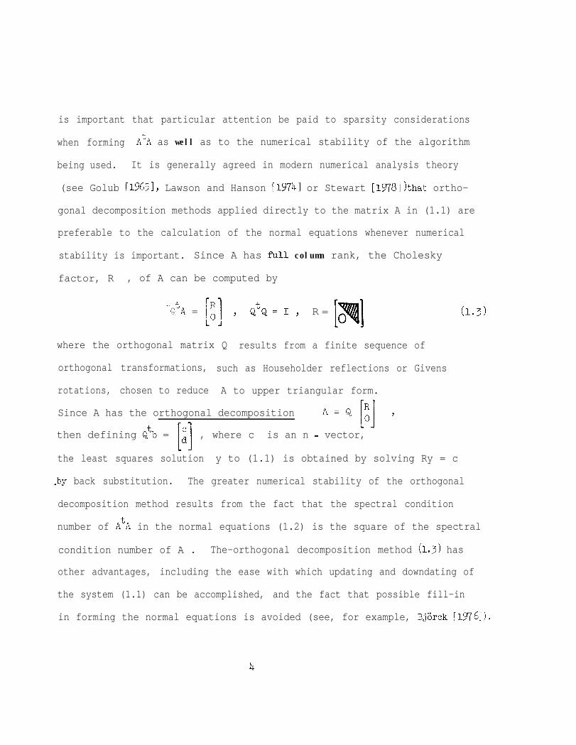
stability is important. Since A has f'ull column rank, the Cholesky

factor, R , of A can be computed by

-Q-tA =TR1 1LO,

7 QtQ=L R = (1.3)

where the orthogonal matrix Q results from a finite sequence of

orthogonal transformations, such as Householder reflections or Givens

rotations, chosen to reduce A to upper triangular form.

Since A has the orthogonal decomposition A=&; 7

then defining Qtb =[I

, where c is an n - vector,

the least squares solution y to (1.1) is obtained by solving Ry = c

-by back substitution. The greater numerical stability of the orthogonal

decomposition method results from the fact that the spectral condition

number of AtA in the normal equations (1.2) is the square of the spectral

condition number of A . The-orthogonal decomposition method (1.3) has

other advantages, including the ease with which updating and downdating of

the system (1.1) can be accomplished, and the fact that possible fill-in

in forming the normal equations is avoided (see, for example, Bj8rck [1976]).

4

However, orthogonal decomposition techniques for solving large sparse

least squares problems such as those in geodesy have generally been

avoided, in part because of tradition and in part because of the lack

of effective means for preserving s.parsity and for managing the

data.

Modern techniques for solving large scale geodetic adjustment

problems have involved the use of a natural form of nested dissection,

called Helmert blocking by geodesists, to partition and solve the normal

equations (1.2). Such techniques are described in detail in Avila and

Tomlin [ 197% in Hanson D9781, and kMeiss1 [1979] where error analyses

are given. ._

The purpose of this paper is to develop an alternative to the formation

and solution of the normal equations in geodetic adjustments. We show how

the orthogonal decomposition method can be combined with a nested dissection

scheme to produce an algorithm for solving such problems that combines

efficient data management with numerical stability.

In subsequent sections the adjustment problem is formulated, and it

is shown how nested dissection leads to an observation matrix A in (1.1)

- of the special partitioned form

A =

./B /’

D4 (1.4)

5

where the diagonal blocks are normally rectangular and dense and where

the large block on the right-hand side is normally sparse with a very

special structure. The form (1.4) is analyzed and a block-orthogonal

decomposition scheme is described. The final section contains some

remarks on the advantages of the a,pproach given in this paper and

relates the concepts mentioned here to further applications. Numerical

experiments and comparisons are given elsewhere in Golub and Plemmons

C 1.98ol.

2. Geodetic Adjustments.

In this 'paper we consider geodetical position networks consisting-_

of mesh-points, called stations, on a two-dimensional reference surface.

Associated with each station there are two coordinates. A line connecting

.two stations is roughly used to indicate that the coordinates are coupled

by one or more physical observations. Thus the coordinates are related

in some equation that may involve, for example, distance formulas or

trigonometric identities relating angle observations. An example of such

a network appears in Figure 1.

FIGURE 1

A 15 station network.

6

More precisely, one considers a coordinate system for the earth

and seeks to locate the stations exactly, relative to that system.

Usually coordinates are chosen from a rectangular geocentric system (see

Bomford [l%'l]). Furthermore, a reference ellipsoid of revolution is

chosen in this set of coordinates and the projection of each station onto

this ellipsoid determines the latitude and longitude of that station.

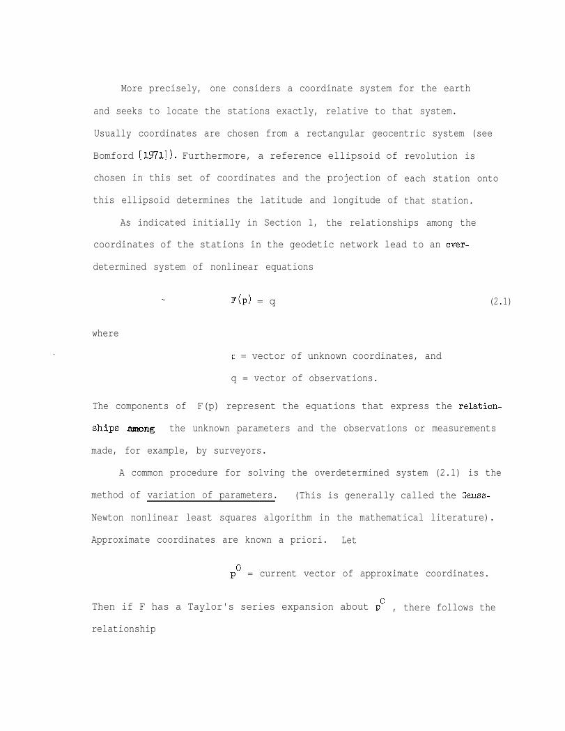
As indicated initially in Section 1, the relationships among the

coordinates of the stations in the geodetic network lead to an over-

determined system of nonlinear equations

F(p) = q (2.1)

where

p = vector of unknown coordinates, and

q = vector of observations.

The components of F(p) represent the equations that express the relation-

shigs mng the unknown parameters and the observations or measurements

made, for example, by surveyors.

A common procedure for solving the overdetermined system (2.1) is the

method of variation of parameters. (This is generally called the Gauss-

Newton nonlinear least squares algorithm in the mathematical literature).

Approximate coordinates are known a priori. Let

PO = current vector of approximate coordinates.

Then if F has a Taylor's series expansion about p" , there follows the

relationship

F(p) = F(p') + F'(p')(p - p") + .,.

where F' (p') denotes the Jacobian of F at p" . Then taking

A = F'(p')

0x = p - p

b = q - F(p")

and truncating the series after 2 terms, one seeks the solution to:

minllb - AX/~ .X

(2.2)

The least squares s-olution y then reapresents the correction to

PO lThat is, one takes

P1 = pO+ y

as the next approximation to p . The process is, of course, iterative

and one can use p1

to compute a further approximation to p . Normally,

the initial coordinates have sufficient accuracy for convergence of the

method, but the number of iterations is often limited by the sheer magnitude

a of the computations. Thus a very accurate approximation to y is desired.

Actually, the equations are usually weighted by use of some positive

diagonal matrix W , where the weights are chosen to reflect the confidence

in the observations: thus (2.2) becomes

min[lW$b - w'Axl12 .X

For simplicity, we will use (2.2) in the analysis to follow. The procedure

8

we discuss, however, will not be complicated by the weights.

Due to the sheer volume of the data to be processed in many

adjustment problems, it is imperative to organize the data in such a

way that the problem can be broken down into meaningful mathematical

sub'problems which are connected in a well-defined way. The total

problem is then attacked by "solving" the subproblems in a topological

sequence. This "substructuring" or "dissection" 'process has been

used by geodesists for almost a century. The method they have employed

dates back to Helmert [1680] and is known as Helmert blocking (see

Wolf [W’81 for a historical discussion).

In Helmert blocking, geogra,phical boundaries for the region in

question are chosen to *partition it into regional blocks. This technique

orders the stations appropriately in order to establish barriers which

divide the network into blocks. The barriers are chosen so that the

interior stations in one block are not coupled by observations to interior

stations in any other block. These interior blocks are separated by sets

of junction stations which are coupled by observations to stations in more

than one block. An example of such a partitioning of the geodetic network

in Figure 1 to one level of Helmert blocking is ,provided in Figure 2.

Here the circled nodes represent the junction stations chosen for this

example.

9

FIGURE 2

One level of Helmert blocking.

The particular form of Helmert blocking we will use here is the same

as that used by Avila and Tomlin [1979] for partitioning the normal

equations. That procedure, in certain respects, is a variation of the

nested dissection method developed by George [1%'3], [1977];

George and Lui [1978];and George, Poole and Voight [X778]. The primary

-emphasis of the nested dissection strategy has been on solving symmetric

positive-definite systems of linear equations associated with finite element

schemes for partial differential equations, There, the finite element nodes

are ordered in such a way that the element matrix B is permuted into

the block partitioned form

10

B =

m

Bl0

0

B2.

. l . .

l .. .

0 0 , . . Bk

Ct

.

C

De

where the diagonal blocks are square.

In our case we use the following dissection strategy in order to

permute the'observation matrix A into the partitioned form (1.4)

Our procedure will be called nested bisection.

Given a geodetical position network on a geographical region 33 ,

first pick a latitude so that approximately one-half of all the stations

lie south of this latitude. This forms two blocks of interior stations

and one block of separator or junction stations and contributes one level

of nested bisection (see Figure 3).

interior stations

junction stations

interior stations

FIGURE 3

One level of nested bisection.

11

I

Now order the stations in IR so that those in the interior regions

A A1

appear first, those in the interior region 2 appear second, and

those in the junction regionB appear last; order the observations

(-l.e., order the equations), so that those‘involving stations in R1

come first, followed by those involving stations inA2 ; then the

observation matrix A can be assembled into the block-partitioned form:

A =

Thus A can be expressed in the block-partitioned form:

A =

.

0

A2

Bl

B2I

where the Aicontains nonzero components of equations corresponding

to coordinates of the interior stations in Jci and where the Bf co&rtain

the nonzero components of equations corresponding to the coordinates ofathe stations in the junction region 23 .

Next, in each of these halves we pick a longitude so that approximately

one-half of the stations in that region lie to the east of that longitude.

This constitutes level 2 of nested bisection. The process can then be

continued by successively subdividing the smaller regions, alternating between

latitudinal and longitudinal dividing lines. Figure 4 illustrates three levels

12

of nested bisection.

A4II A YIfm-M- ----P -- --c--e

A 7FIGURE 4

Three levels of nested bisection.

The observation matrix associated with the nested bisection of the

geodetical position network in Figure 4 can then be assembled into the

Eld5

lizId 6

IT3d7

I!3A8

l (2.3)

13

It follows that if nested bisection is carried out to k levels,

then the patiltioned form of the assembled observation matrix has:

i> pk diagonal blocks associated withinterior regions, and

ii>k2 -1 blocks associated with junction regions.

In particular, there are

iii) 2k-l junction blocks which are each coupled to2 interior regions, and

iv) 2k-1

-1 junction blocks which are each coupled to4 interior regions.

Heuristically, one normally would like to perform the bisection

process so that the sets of junction stations are minimal at each level,

'thus maximizing the numbers of columns in the diagonal blocks. The process *

is stopped at the level k at which the 2k diagonal blocks are suffi-

ciently dense or at the level at which further subdivisions are not

feasible or are not necessary for the particular adjustment problem.

Our proposed block Jrthogonal decomposition algorithm for an obser-

vation matrix A already in the partitioned form determined by nested-

bisection is deferred to the next section.

3. The Block Orthogonal Decomposition.

In this section we describe a block orthogonal decomposition algorithm

for solving the least squares adjustment problem minl(b-Axi12 , whereX

the observation matrix A has been assembled into the general block

diagonal form (1.4). Here we assume that the structure of A is specified

by the nested bisection scheme described in Section 2. Other dissection

14

schemes may be preferable in certain applications (see Golub and

Plemmons [X980]).

We first illustrate the method with k = 2 levels of nested

bisection, as given in Figure 5.

FIGURE 5

Two levels of nested bisection.

Suppose that the associated observation matrix A is assembled into the

corresponding block-partitioned form, giving

A =

'Al

.

Bl Dl

A2 B2 D2

A3 c3 D3

. A4 c4 D4,

Then by the use of orthogonalization techniques based upon, for example,

Householder reflections, Givens rotations or modified Gram-Schmidt ortho-

gonalization, the reduction of A to upper triangular form proceeds as

follows:

15

At the first stage, each diagonal block

orthogonal transformations.

Ai is reduced by

Here the Q.1 are orthogonal

be formed explicitly) and Qi Ai

matrices (which of course need not

= , where R. =1 , yielding

,

Rl

0

R2

0

R30

R4

0.

B01 DO 11

BlD11

B02 DO 21

B2 D12

Co Do3 3

1 1c4 9c

The row blocks corresponding to the upper triangular matrices Ri

are then merged through a permutation of the rows9 yielding

16

Rl

R2

B01 DO 1

B02

DO2

R3Co Do

3 3

R4 C; D"

Bl 1 1Dl

1B2 D1

2

C1 D13 3

C; D'.

.

This completes the first stage of the reduction. For the intermediate

stages, pairs of merged blocks corresponding to junction stations are

reduced. First,E] and [$]

are reduced to upper triangular

form by orthogonal transformations, yielding

.

Rl

R2

R3

.

0Bl

DO1

B02

DO2

Co Do3 3

R4 C; D;

R5DO

5

0 D15

R6 ‘:

0 Di

.

17

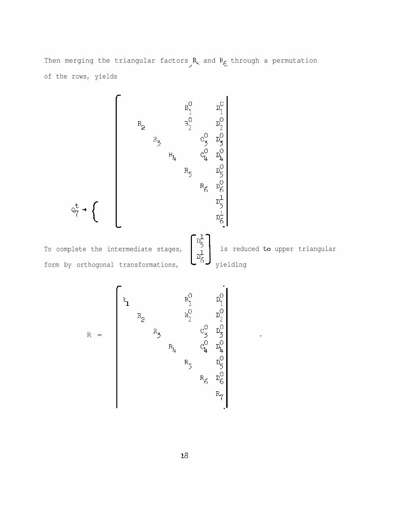
Then merging the triangular factors R, and R, through a permutation/ ”

of the rows, yields

R2

R3

B01

DO1

B02

DO2

Co Do3 3

R4 C; D;

R5DO

5

R6 ':

D151

D6m

To complete the intermediate stages,

form by orthogonal transformations,

D15[3Di is reduced to upper triangular

yielding

R =

3

R2

.

B01

DO1

B02

DO2

R3Co Do

3 3

R4 C4" D;

R5DO

5

R6 ':

18

Here R is the Cholesky factor for A . Let ni denote the

torder of R denote thei for i = l,...,?' and let ct = (c1J . . ..c >

7‘

result of applying the same sequence of orthogonal transformations and

permutations to b , where each c. is an n -vector.1 i

For the final

step of the solution process, the least squares solution y to Ax ~b

is computed as follows.

Partition y as yt = (yl,...,y71t where yi is an n -vector,i

i = l,..., 7. Then the following upper triangular systems are solved

successively by back-substitution for the vectors y. , i = 7,6,...,1 .1

Riyi = ci - Dpy7 ) i = 6,5,

Riyi = Ci - C;y6 - Dyy7 j i = 4,3,

Riyi = ci - B;y5 - DPY7 7 i = 2,l.

The general reduction process is described next in terms of three

basic steps. Let A and b denote the observation matrix and vector

resulting from k levels of nested bisection of a geodetic position

network on some geographical region. Assume that A has been assembled

into the general block-partitioned form (1.4), with 2k diagonal blocks

and 2k-l remaining column blocks. Letting t = 2k , we write A as

19

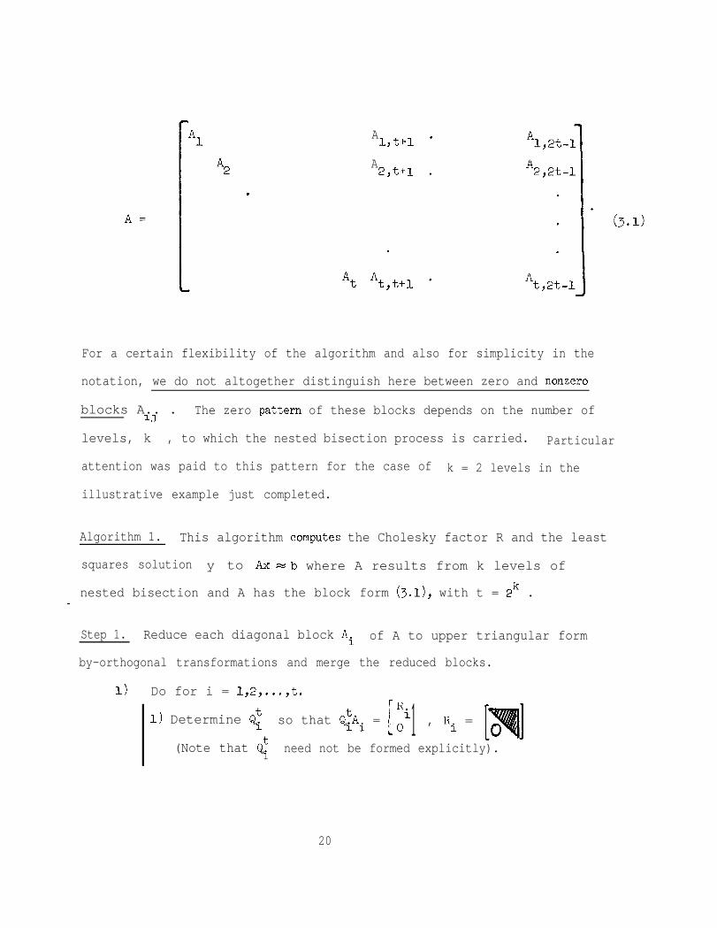
A1,t+1 '

A2,t+1 l

For a certain flexibility of the algorithm and also for simplicity in the

notation, we do not altogether distinguish here between zero and nonzero

blocks A.. .1J

The zero ,pattern of these blocks depends on the number of

levels, k , to which the nested bisection process is carried. Particular

attention was paid to this pattern for the case of k = 2 levels in the

illustrative example just completed.

Algorithm 1. This algorithm com,putes the Cholesky factor R and the least

squares solution y to Ax -b where A results from k levels of

nested bisection and A has the block form (3.11, with t = 2k .-

Step 1. Reduce each diagonal block Ai of A to upper triangular form

by-orthogonal transformations and merge the reduced blocks.

1) Do for i = 1,2,...,t.

1) Determine Qi 1so that Q& = tR.1

LO 1 , Ri =

(Note that Qti need not be formed explicitly).

20

2) Compute

t%[. Ai,Ai t+l,"',Ai 2t 117 7 -

.Ri

A;7 t+l.. .

A;7 2t

.;-

0 A:- 7

t+l... A:72t 1-aI .

2) Merge the reduced row blocks by row permutations so that the

resulting matrix has the form

A01,t+1 A01,t+2

A02,t+1

A02,t+2

. .

, . . AF,3t/2

, . .A&/2

A&t/2)+1 l

A;,(3t/2)+1 l

1Al,t+l

A12,t+1

A13,t+2

A41, t+2

1

. . A01,2t-10. . A2,2t-l

.

. .

.

. . A0t,2t-1

. l A11,2t-1

. l A12,2t-1

. . A13,2t-1

. . Aql,gt-1

.

.

.

A1t-1,2t-1

l . At,2t-l

21

step 2. Reduce and merge the intermediate-stage blocks.

1) Do for u = t, t/2,..., t/2k-l= 2 .

1) Do for v = 1,3,...,u-1

1)

2)

Reduce each pair of row diagonal blocks

[

A1WJ-V

A1v+1,t

to upper triangular form by orthogonal transformation,

as in Step 1.

Merge the resulting reduced row blocks by row permutations

so that the upper triangular blocks R.1

appear first, as

in Step 1.

At the end of Step 2, A has been reduced by orthogonal transformations

to the following form, where each Ri is upper triangular and where certain

of the blocks A0ij are zero.

22

A01,t+1 l

0

A2,t+l l

. l

Rt

0

At,t+l '

Rt+l

. (3.2)

Step 3. Back Substitution. Let ni denote the order of Ri , for

ti = 1,...,2t-1 . Let ct = (c~,...,C~~-~ > denote the result of

applying the same sequence of orthogonal transformations to b and let

Yt = (y1' ...,Y~~ l)t denote the least squares solution to Ax xb ,

where c and yi are n.-vectors, i = 1,...,2t-1. Solve each of thei 1

following upper-triangular systems by back-substitution

1) R2t-lY2t-l = C2t-1

2t-12) R.y =

li ci - 1 A0 Y j 7 i =ij

2t-2, 2t-1,...,t

j=ii-1

2t-1

3) Riyi=ci- Ayj Yj 7 i = t7 t-17***71 l

j=t+l

23

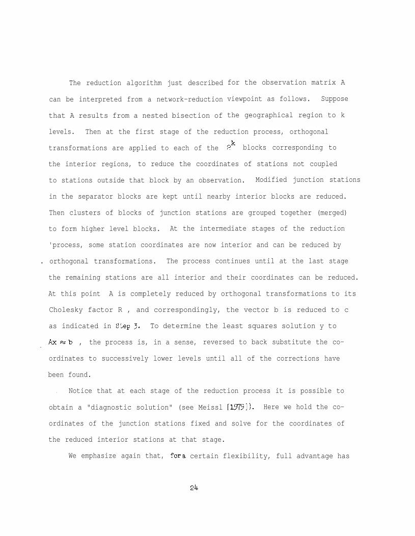
The reduction algorithm just described

can be interpreted from a network-reduction

that A results from a nested bisection of

for the observation matrix A

viewpoint as follows. Suppose

the geographical region to k

levels. Then at the first stage of the reduction process, orthogonal

transformations are applied to each of the 2k blocks corresponding to

the interior regions, to reduce the coordinates of stations not coupled

to stations outside that block by an observation. Modified junction stations

in the separator blocks are kept until nearby interior blocks are reduced.

Then clusters of blocks of junction stations are grouped together (merged)

to form higher level blocks. At the intermediate stages of the reduction

'process, some station coordinates are now interior and can be reduced by

. orthogonal transformations. The process continues until at the last stage

the remaining stations are all interior and their coordinates can be reduced.

At this point A is completely reduced by orthogonal transformations to its

Cholesky factor R , and correspondingly, the vector b is reduced to c

as indicated in Ste.p 3. To determine the least squares solution y to

Axxb , the process is, in a sense, reversed to back substitute the co--

ordinates to successively lower levels until all of the corrections have

been found.

. Notice that at each stage of the reduction process it is possible to

obtain a "diagnostic solution" (see Meissl [1979]). Here we hold the co-

ordinates of the junction stations fixed and solve for the coordinates of

the reduced interior stations at that stage.

We emphasize again that, fora certain flexibility, full advantage has

24

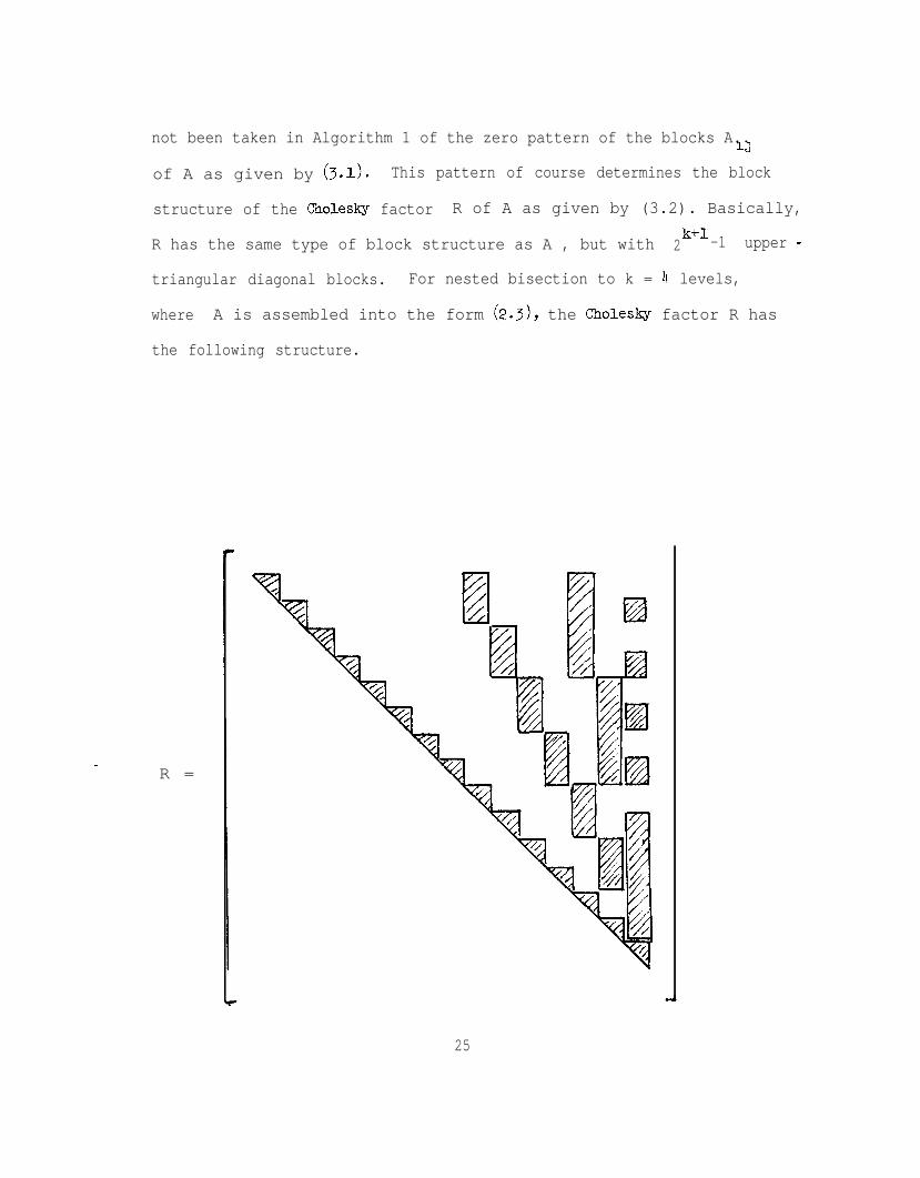
not been taken in Algorithm 1 of the zero pattern of the blocks A..1J

of A as given by (3.1>* This pattern of course determines the block

structure of the Cholesky factor R of A as given by (3.2). Basically,

R has the same type of block structure as A , but with 2k+l-1 upper -

triangular diagonal blocks. For nested bisection to k = 4 levels,

where A is assembled into the form (2.31, the CholesQ factor R has

the following structure.

-R =

25

In order to facilitate an analysis of the results of a least

squares adjustment, it is often desirable to compute some or all of

the elements of the variance-covariance matrix @A )-1

l Since

(ADA)-' = (R~R)-' ,

the special block structure of R just discussed can be used advanta-

geously in computing the variances and covariances. Such a procedure

is given in the next section for a more generally sparse Cholesky factor R .

4. Computation of the Variances.

In many adjustment problems (see, for example, Hanson [1978]) it is

necessary to compute the variances and covariances associated with the

regression coefficients in order to estimate the accuracy of the results.

Under the usual assumptions, the variance of the i-th coefficient is pro-

portional to the (i,i> element of (~~~1-l . If R is sparse, then the

diagonal elements of (A~AP can be calculated quite efficiently. Indeed,

it is easy to compute all the elements of (Ate)-' which are associated

with the non-zero elements of R , the Cholesky factor. We describe the-procedure next.

Using the orthogonalization algorithm we determine the Cholesky

factor R so that

Suppose

AtA = RtR ,

r ij f 0 when (i,j)e K

= 0 when (i,j)k K .

26

Our objective is to determine

((ADA?-] ijWhen (i,j) E: K ,

Let us write

(A%' = z = [zl,...,z,l ,

where zi is the i-th column of the matrix Z .

SinceL

A'AZ = I

RZ = (R?-' .

Note that =

((Rt)-+ii = 1 / rii .

From (4.1) and (4.2), we see that

R zn = en X (r&-1

( ei = (0 ,...,O,l)

so that we can solve for zn by back substitution. Thus

Znn = (rmY2

and for i = n-l,n-2,...,1

n nr r

Z = -1

ij zii jn = -

ij zin r L jn l

j=i+lj=i+l rii

(4.1)

(4.2)

(i,j)E K

27

Let In = min c Ii r f 30 . It is possible to calculate1 < i < n-l in- -

Z ;n for i = n-l,n-2,...,1- . Once these components have been computed,111 11

it is only necessary to save those elements for which (i,n) E

Note

Z = Z .in ni

Now assume we have calculated those elements of zn,zn 1,

for which

K .

� l 7zj +1

rPqf 0 when p=l,...,n ; q = B+l,..,n .

IThus, by symmetry we have computed

z@for q > 1 and (!,qk K .

Now for i = 1,2,., 1-l

n

trij 'j,i!

= 0

j=i

ande

H.ence

n

11

j=j

'1.j 'ja = rli l

n

L(-L- _‘1R = rlj z

r >51 Rj 'je

j=l+l

n

( IL-- x 151 ‘ej ‘&

j=1+1

28

Let I1 = min c Ii riR f 30 .15 i< 8-l

Then for i = P-l,...,IR

-

azi4 = ( -

1rij Zja - f r

ij '13,> / r

ii 'j=i+l j=&+l

(i,j)e K . (i,j)e K

Again, after this 'calculation is performed, we save only those elements

for which (i,a) E K . The above algorithm thus describes a method for

computing the elements of the inverse of (AtA) which are associated

with the non-zero elements of R . Such a procedure can be quite

efficient when compared to computing

(ADA)-' = R-l(Rt)-' .

For example, suppose we need the diagonal elements of (AtA)-' when

rij f 0 for i = j and j = i+l , and

rij = 0 otherwise,

i.e. R is bi-diagonal. The matrix R-1 will be completely filled in

above the diagonal and hence O(n2) numerical operations are required to

compute the diagonal elements of (Ate)-1 a The algorithm we have outlined

above would require O(n) operations. Even greater savings can be expected

. for the Cholesky factor R of the form (3.2), resulting from nested bi-

section.

5. Final Remarks.

To summarize, an alternative has been provided here to the formation

and solution of the normal equations in least squares adjustment problems.

In particular, it has been shown how a block-orthogonal decomposition method

29

can be used in conjunction with a nested dissection scheme to provide

a least squares algorithm for certain geodetic adjustment problems,

Some well-known advantages ofdissectionschemes for sparse linear systems

are that they facilitate efficient data management techniques, they allow

for the use of packaged matrix decomposition routines for the dense

component parts of the problem,and they can allow for the use of parallel

processing. In the pas-&the combination of the normal equations approach

with these dissection techniques (in particular Helmert blocking) has been

preferred, partly because of tradition and partly because of the simplicity

and numerical efficiency of the Cholesky decomposition method. However,

the use of an orthogonal decomposition scheme applied directly toan

observation matrix A which has also been partitioned by a dissection

. scheme has several advantages over the normal equations approach. First,

the Q,R orthogonal decomposition of A allows for an efficient and

stable method of adding observations to the data (See Gill, Golub, Murray

and Saunders [lg'&]). Such methods are crucial in certain large-scale

adjustment problems (see Hanson [lfl8]). Secondly, possible fill-in that

can occur in forming the normal equation matrix AtA is avoided. A-

statistical study of such fill-in is .provided by Bjorck [1976]. Meissl

[1979] reports that some fill-in can be expected in forming AtA in the

readjustment of the North American Datum. This problem cannot be over-

emphasized in such large scale-systems (~,OOO,OOO equations and 4GO,GOG

unknowns). But perhaps the most crucial advantage of the use of ortho-

gonal-decomposition schemes here is that they may reduce the effects of

ill-conditioning in adjustment calculations.

30

In this 'paper we have treated only one aspect of nested dissection

in least squares problems, that of decomposing a geodetical position

network by the 'process of nested bisection. However, the block diagonal

form of the matrix in (1.4) can arise in other dissection schemes such

as one-way dissection (see George, Poole and Voight [lfl8] for a description

of this scheme for solving the normal equations associated with finite

element problems). The form also arises in other contexts, such as photo-

grammetry (See Golub, Luk and Pagan0 [l%'g]). Least squares schemes based

in part upon block iterative methods (see Plemmons [1979])or a combination

of direct and iterative methods may be preferable in some applications.

Moreover, the general problem of permuting A into the form (1.4) by

some graph-theoretic algorithm for ordering the rows and columns of A

(see Weil and Kettler [lY'Tl]) has not been considered in this 'pa'per.

Some of these topics will be addressed further in Golub and Plemmons [1980].

31

REFERENCES

V. Ashkenazi [1971], "Geodetic normal equations", in Large Sets of LinearEquations , J. K. Reid, ed., Academic Press, NY, 57-74.

J. K. Avila and J. A. Tomlin [1979], "Solution of very large least squaresproblems by nested dissection on a parallel processor", Proc. ofComputer Science and Statistics: Twelfth Annual Symposium on theInterface, Waterloo, Canada.

A. Bj8rck [1976], "Methods for sparse linear least squares ,problems", inSparse Matrix Computations, J. R. Bunch and D. J. Rose, eds., AcademicPress, NY, 177-194.

G. Bomford [1971], Geodesy, Clarendon Press, Oxford, Third Edition.

A. George [1973 1, 'Nested dissection on a regular finite element mesh',SIAM J. Numer. Anal. 10, 345-363.

A. George [1977], "Numerical experiments using dissection methods to solven by n grid problems", SIAM J. Numer. Anal. 14, 161-179.

A. George and J. Liu [1978], "Algorithms for matrix partitioning and thenumerical solution of finite element systems', SIAM J. Numer. Anal. 15,2%32'7.

A. George, W. Poole and R. Voigt [1978], 'Incomplete nested dissection forsolving n by n grid ,problems", SIAM J. Numer. Anal. 15, 662-673.

P. E. Gill, G. H. Golub, W. Murray and M. A. Saunders [19"&], "Methods forupdating matrix factorization", Math. Camp. 28, 505-535.

G. H. Golub [1965], "Numerical methods for solving linear least squaresproblems", Numer. Math. 7, 206-216.

sG. H. Golub and R. J. Plemmons [1980], 'Dissection schemes for large sparse

least squares and other rectangular systems', in preparation.

G:H. Golub, F. T, Luk and M. Pagan0 [1979], "A sparse least squares problem_ in photogrammetry", Proc. of Computer Science and Statistics: Twelfth

Annual Conference on the Interface, Waterloo, Canada.

R. H. Hanson [1978], " A posteriori error propogation", Proc. Second Symposiumon problems related to the redefinition of North American GeodeticNetworks,Washington, DC, 427-445.

F. R. Helmert [1880], Die mathematischen und p'hysikalischen Theorien derh6heren Geodasie,

--_1 Teil, Leipzig, Germany.

32

G. B. Kolata [19’78], "Geodesy: dealing with an enormous computer task",Science 200, 421-422, 466.

Ce Lo Lawson and R. J. Hanson [1974], Solving Least Squares Problems,Prentice Hall, Englewood Cliffs, NJ.

P. Meissl [19'79], "A priori prediction of roundoff error accumulationduring the direct solution of super-large geodetic normal equations",NOAA Professional Paper, Department of Commerce, Washington, DC.

R. J. Plemmons [19'79], "Adjustment by least squares in Geodesy using blockiterative methods for sparse matrices", Proc. Annual U. S. Army Conf.on Numer. Anal. and Computers,El Paso, TX.

G. W. Stewart [1%'7], "Research, development and LINPACK?, in MathematicalSoftware II , J. R. Rice, ed., Academic Press, N.Y.

R- L. Weil and P. C. Kettler [ 1971], "Rearranging matrices to block-angular form for decomposition (and other) algorithms", ManagementScience 18, 98-108.

H. wolf [19783, "The Helmert block method - its origin and development",Proc. Second SvmDosium on Problems Related to the Redefinition ofNorth American"Geodetic Networks, Washington, DC, 319-325.

33

1I