large-scale fermentation of e. coli for the production of
TRANSCRIPT

University of Pennsylvania University of Pennsylvania
ScholarlyCommons ScholarlyCommons
Senior Design Reports (CBE) Department of Chemical & Biomolecular Engineering
4-2016
Large-Scale Fermentation of E. Coli for the Production of High-Large-Scale Fermentation of E. Coli for the Production of High-
Purity Isoprene Purity Isoprene
Phillip A. Taylor University of Pennsylvania, [email protected]
Yuta Inaba University of Pennsylvania, [email protected]
Ian J. Pinto University of Pennsylvania, [email protected]
Follow this and additional works at: https://repository.upenn.edu/cbe_sdr
Part of the Biochemical and Biomolecular Engineering Commons
Taylor, Phillip A.; Inaba, Yuta; and Pinto, Ian J., "Large-Scale Fermentation of E. Coli for the Production of High-Purity Isoprene" (2016). Senior Design Reports (CBE). 79. https://repository.upenn.edu/cbe_sdr/79
This paper is posted at ScholarlyCommons. https://repository.upenn.edu/cbe_sdr/79 For more information, please contact [email protected].

Large-Scale Fermentation of E. Coli for the Production of High-Purity Isoprene Large-Scale Fermentation of E. Coli for the Production of High-Purity Isoprene
Abstract Abstract We present a process for the production of isoprene via the fermentation of glucose. Based on our current specifications, we conclude that the use of recombinant E.coli for the fermentation of glucose is a novel yet unprofitable venture. Our current design entails the continuous production of isoprene using 3 pre-seed, 3 seed, and 5 production fermenters each with a production fermentation time of 72 hours. Our scheduling of the fermenters allowed us to produce isoprene continuously at a steady rate, and the liquid by-products of the fermentation were removed and sterilized at the end of each batch. Isoprene was mainly present in the vapor phase during the fermentation and was purified using a combination of an absorption using ISOPAR v, stripping with steam, and separation using a flash vessel.
It was desired that the fermentation was operated near the minimum oxygen concentration (MOC) as such conditions allowed for the highest production rate of isoprene based on the preliminary studies done by Chotani in their patent. The fermentation was operated at 34 °C and 1.7 bar with glucose and oxygen as the reactants producing isoprene, carbon dioxide, and water as the products.
The results of our design suggest that the price of isoprene is too low when compared to the costs of raw materials, making this process economically unfeasible under present market conditions. We project that $4.08 worth of glucose will be need for each pound of isoprene which currently goes for $0.79/lb. Additionally, the metabolic pathway of isoprene is highly exothermic, requiring large utility requirements in terms of chilled water to remove heat from the fermenters. We are unsure of impacts of rapidly changing the temperature of E.Coli on production as there is no data regarding the robustness of the strain. Overall, the fixed capitals costs incurred make this process even more unappealing for further consideration.
Disciplines Disciplines Biochemical and Biomolecular Engineering | Chemical Engineering | Engineering
This working paper is available at ScholarlyCommons: https://repository.upenn.edu/cbe_sdr/79
April 12th, 2016
Dear Dr. Fabiano, Dr. Bockrath and Dr. Bidstrup-Allen,
Our team submits the following design proposal for the project of using a fermentation
process for the production of isoprene. We thank you for your continued guidance over the
semester in completion of this design.
The following design used hand calculations to make the initial estimates for the
equipment sizes and material balances. Aspen v8.8 was use to take these initial estimates and
fine tune various parameters required in the process to close the loops to recycle and conserve
materials. Since Aspen does not handle batch processes well, the key processes involving the
fermenters were designed with the aid of Excel.
While the overall plant design is complete, external market forecasts are a significant
factor for making the managerial decision to pursue this joint venture. We project that this design
will not become profitable unless industry conditions drastically change the price of glucose or
isoprene. Isoprene prices are too low as a commodity chemical to justify the use of a biological
process at this time.
Sincerely,
Phillip Taylor
Yuta Inaba
Ian Pinto

2
Large-scale Fermentation of E.coli for the Production of
High-Purity Isoprene
Yuta Inaba1, Ian Pinto1, Phillip Taylor1
1 – Department of Chemical and Biomolecular Engineering, University of
Pennsylvania
220 South 33rd Street, Philadelphia 19104

3
Table of Contents
Abstract Introduction and Objective Time Chart Market and Competitive Analysis Preliminary Process Synthesis Assembly of Database Process Flow Diagram and Material Balance Process Description Energy Balance and Utility Requirements Equipment List and Unit Descriptions Specification Sheets Equipment Cost Summary Fixed-capital Investment Summary Operating Cost Other Considerations Profitability Analysis Conclusion and Recommendation Acknowledgements Bibliography Appendix
4 5-6 7-8
9-11 12
14-16 17-21 22-23 24-37 38-46
47 48
49-51 52-56 57-59 60-61
62 62
63-79

4
Abstract We present a process for the production of isoprene via the fermentation of glucose.
Based on our current specifications, we conclude that the use of recombinant E.coli for the
fermentation of glucose is a novel yet unprofitable venture. Our current design entails the
continuous production of isoprene using 3 pre-seed, 3 seed, and 5 production fermenters each
with a production fermentation time of 72 hours. Our scheduling of the fermenters allowed us to
produce isoprene continuously at a steady rate, and the liquid by-products of the fermentation
were removed and sterilized at the end of each batch. Isoprene was mainly present in the vapor
phase during the fermentation and was purified using a combination of an absorption using
ISOPAR v, stripping with steam, and separation using a flash vessel.
It was desired that the fermentation was operated near the minimum oxygen
concentration (MOC) as such conditions allowed for the highest production rate of isoprene
based on the preliminary studies done by Chotani in their patent. The fermentation was operated
at 34 °C and 1.7 bar with glucose and oxygen as the reactants producing isoprene, carbon
dioxide, and water as the products.
The results of our design suggest that the price of isoprene is too low when compared to
the costs of raw materials, making this process economically unfeasible under present market
conditions. We project that $4.08 worth of glucose will be need for each pound of isoprene
which currently goes for $0.79/lb. Additionally, the metabolic pathway of isoprene is highly
exothermic, requiring large utility requirements in terms of chilled water to remove heat from the
fermenters. We are unsure of impacts of rapidly changing the temperature of E.Coli on
production as there is no data regarding the robustness of the strain. Overall, the fixed capitals
costs incurred make this process even more unappealing for further consideration.

5
Introduction and Objective Time Chart
This design project originates from analyzing whether the Dupont/Goodyear joint venture
to manufacture isoprene using the fermentation of sugar is a viable approach to compete with
traditional petrochemical manufacturing processes. A plant design using this process will be
detailed to see whether this process is economically viable for these companies.
Table 1 displays the initial charter for this project addressing the breadth and depth of the
analysis presented.
Table 1: Project Charter
Project Name:
Isoprene production from fermentation of E.Coli on sugar
Specific Goals:
Design a plant for this process at an industrial-scale for economic analysis
Project Scope:
In-scope
Using patented information as estimates of the production rates and production
platform
Evaluating different design alternatives to minimize cost while maintaining feasibility
Evaluate profitability of the process or lack thereof and find the most significant
factors that affect the viability of the process
Out-of-scope
Attempting to propose other platforms and methods to biologically produce isoprene
6
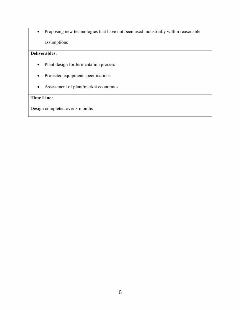
Proposing new technologies that have not been used industrially within reasonable
assumptions
Deliverables:
Plant design for fermentation process
Projected equipment specifications
Assessment of plant/market economics
Time Line:
Design completed over 3 months

7
Market and Competitive Analysis
Since January 2012, the U.S. import price for isoprene has been pushed downwards from
prices upwards of the $3500/ton range to prices around $1500/ton in mid-2015. The price of
isoprene is generally bounded by the price of rubber. The price of rubber (RSS3 grade) peaked in
early 2011 at roughly $2.70/lb of rubber. The increased production of natural rubber in Asia has
oversupplied the market and currently remains at $0.70/lb (Figure 1). On top of increased supply
of natural rubber, the demand for rubber has fallen as China’s historically strong growth slowed.
With China’s economy expanding much more slowly, consumption of rubber and isoprene will
not see much growth until 2020 as the market readjusts for the excess inventories of rubber1.
Figure 1. Monthly rubber prices per pound
As for the market for isoprene monomer in North America outside of synthetic rubber, a
majority of imported isoprene is polymerized to form adhesives. While imports have increased
1 http://www.bloomberg.com/news/articles/2015‐03‐23/world‐rubber‐demand‐slowdown‐seen‐weighing‐on‐price‐through‐2020

8
significantly since 2008, many businesses are choosing to buy isoprene from markets where
rubber prices have influenced isoprene spot sales.
The price for natural rubber remains a fairly good estimate for high-purity isoprene to be
produced in this process as 70% of isoprene was polymerized for end-use in tires in 20132.
Therefore, natural rubber prices must recover for isoprene prices to increase again.
Furthermore, isoprene is currently produced as a byproduct of catalytic cracking in
petrochemical processes. With low crude oil prices forecasted over the next several year,
isoprene will remain relatively cheap to produce using traditional approaches. Roughly 800,000
tons of petrochemical isoprene is polymerized to cis-polyisoprene each year.
2 https://www.ihs.com/products/isoprene‐chemical‐economics‐handbook.html

9
Preliminary Process Synthesis
The production of isoprene via fermentation requires a minimum oxygen concentration
(MOC) of 9.97%. During the early stages of the process synthesis, there were two flow sheets
which satisfied this requirements.
Option A: Air can be used as the source of oxygen and N2 gas can be used as a diluent.
Option B: The fermenter-off gases can be recycled and mixed with air so that the MOC is
satisfied.
The objective was to operate the fermentation near the MOC since it allowed for the
highest rate of production of isoprene as referenced by one of our patents, US 2011/0178261 (2.2
g/hr-L).
1. Use of Nitrogen Gas as a Diluent
The reaction pathways for both Options A and B were the same. The nitrogen gas would
have to be obtained from a cryogenic plant and this option was ruled out due to the large
volumes of nitrogen gas that would be required for the dilution. The alternative—i.e. option B—
was determined to be favorable since it did not require the use of a diluent. Assuming the N2 flow
rate assumed below, 31,531,130 SCFH of nitrogen flow would be required. From Airgas’
website, a Cryo-turbine plant would have a maximum capacity of 400,000 SCFH3. To meet our
diluent requirements, 8 cyroplants would be required to supply enough air. These plants would
3 https://www.airgas.com/medias/305‐On‐Site‐Nitrogen‐System‐Services.pdf?context=bWFzdGVyfHJvb3R8NzA2Njg1fGFwcGxpY2F0aW9uL3BkZnxoMmMvaDI1LzkwNzY5MjcyMDEzMTAucGRmfGMzYjI1YWM1Zjc5ZWUyZmZiMzRjOWRlNDM5NmU2YTE1Y2JmNmE3NWY3MTdhY2VjYmNlODA4ZmUyZTc5NmNjMWE

10
also incur heavy land costs and operating expenses as well as a large fixed capital investment.
Therefore, this option was not pursued any further.
Figure 2.1 Unit operations for the dilution of air with N2 gas (Option A)
2. Recycling of the Fermenter-off Gases
Option B involves the recycling of the fermenter-off gases. The fermenter off gases first
enter an absorption column where the isoprene is absorbed from the gas phase. The remaining
gas components which are mainly incondensable gases then leave the absorption column. This
gas stream is split to purge some of the gases and the remainder is mixed with the air stream to
be fed to the fermenter.
It is also important to note that a fraction of the vapor stream that is leaving the
absorption column has to be purged. There are several inerts in the process such as nitrogen and
argon. To avoid any accumulation of these inerts in the system, a fraction of the vapor stream has
to be purged before it’s mixed with the feed gas.
Mixer Fermenter To
Absorption
Column
Air
215,233 lb/hr
N2
232,057 lb/hr
Mixed Stream
447,291lb/hr
9.97 vol % O2
Fermenter‐Off
Gases
Glucose
127,632 lb/hr

11
Figure 2.2 Unit operations for the dilution of air by recycling the fermenter‐off gases (Option B)
Absorption
Column
Splitter
Air
280,564 lb/hr
Vapor
Product
Liquid
Product
Purge
Stream Recycle
Stream
Glucose
127,632 lb/hr
9.97 vol %
O2 Mixer Fermenter

12
Assembly of Database
The heat capacities, boiling points, molecular weights, and toxicity data were obtained for
all of the components as the relevant thermophysical properties in the process. Based on the
results of US 2011/0178261, the isoprene producing strain CMP1043 of E.coli will produce
isoprene at the following rate with the reaction:
Rate of isoprene production = 2.2 g/hr-L (where L represents per L of broth volume) using the
pathway,
C6H12O6 + 3.41 O2 = 0.370 C5H8 + 4.15 CO2 + 4.52 H2O.
Table 2: Thermophysical Properties, Toxicity, and Price of Principal Chemicals
Component Cp at 25°C (J mol-1 K-1)
Boiling Point (°C)
MW (g/mol)
Price (per lb)
Isoprene 144.75 34 68.12 $0.79
Oxygen 29.10 -183 16 N/A
Glucose 218.6 410.8 180.16 $0.40
Carbon Dioxide
29.10 -78.5 44.01 N/A
Water 4184 100 18.02 $0.20/m3
Nitrogen 29.10 -195.8 14.01 N/A
Argon 20.79 -185.8 39.95 N/A Isopar $0.64
Note: Any prices which were listed as N/A were not used in the profitability analysis. These
components were either by-products (for example, water) or were raw materials that were
obtained from ambient air.

13
The by-products could not be sold due to their low purities and thus they were excluded from the
profitability analysis. We also assumed the extracellular production of other compounds were
minimal using a biological pathway. Also, the heat capacities for oxygen, carbon dioxide,
nitrogen, and argon were computed assuming ideal gas behavior.

14
Process Flow Diagram and Material Balance
Our process flow diagram and a break‐down of stream properties within the process is
show below.
Figure 3. Process Flow Diagram

15
Table 3.1. Material Balance Block
Stream Number
11 12 13 14 15 16 17 18 19 20
Temperature (°C)
15 30 34 34.18 34.18 34.18 34.85 115.61 107.75 98.39
Pressure (bar)
1.01 1.01 1.7 1.7 1.7 1.7 1.7 1.7 1.7 1.7
Vapor fraction
0 0 0 1 1 1 0 1 0 1
Mass flow (lb/hr)
23,796,890 58,731.2 3,373,580 665,975 322,998 342,977 3,391,740 337,594 3,693,380 35962.34
Molar flow (lbmol/hr)
1,320,875.34 3260.07 18298.37 21395.76 10376.94 11018.81 18616.27 18739.29 36128.68 1226.881
Component molar flow:
(lbmol/hr)
Isoprene 0 0 0 3.90 1.89 2.01 215.25 0 3.83E-18 215.25
Oxygen 0 0 0 697.49 338.28 359.21 1.566 0 5.97E-48 1.566
Glucose 0 0 0 0 0 0 0 0 0 0
Carbon Dioxide
0 0 0 4242.27 2057.50 2184.77 57.944 0 1.93E-29 57.94
Water 1,320,875.34 3260.07 0 667.85 323.90 343.94 19.089 18739.29 17838.89 919.49
Nitrogen 0 0 0 15596.23 7564.17 8032.06 24.324 0 3.91E-50 24.32
Argon 0 0 0 186.33 90.37 95.96 0.542 0 3.62E-50 0.542
Isopar 0 0 18298.37 1.677 0.813 0.864 18297.55 0 18289.79 7.765
Stream Number
1 2 3 4 5 6 7 8 9 10
Temperature (°C)
25 90.85 80 34 34.09 34 25 34 34 5
Pressure (bar)
1.01 1.7 1.01 1.7 1.7 1.7 1.7 1.7 1.7 1.01
Vapor fraction
1 1 0 1 1 0 0 1 0 0
Mass flow (lb/hr)
280,565 280,565 58,731.2 280,565 623,543 127,632 8,893,900 678,632 8,893,900 23,796,890
Molar flow (lbmol/hr)
9686.67 9686.67 3260.07 9686.67 20705.49 2621.31 493,550 21,597 493,550 1,320,875.34
Component molar flow:
(lbmol/hr)
Isoprene 0 0 0 0 2.01 0 1.46 185.5 1.46 0
Oxygen 2029.4 2029.36 0 2029.3 2388.6 0 0.54 697.5 0.54 0
Glucose 0 0 0 0 0 495.91 0 0 0 0
Carbon Dioxide
2.62 2.62 0 2.6154 2187.4 0 78.78 4244.81 78.78 0
Water 0 0 3260.07 0 343.9 2125.399 493,462.97 685.74 493,462.97 1,320,875.34
Nitrogen 7564.32 7564.32 0 7564.32 15596.4 0 6.29 15596.34 6.29 0
Argon 90.38 90.3766 0 90.3766 186.3 0 0.16 186.34 0.16 0
Isopar 0 0 0 0 0.863 0 0.01 0.864 0.01 0
16
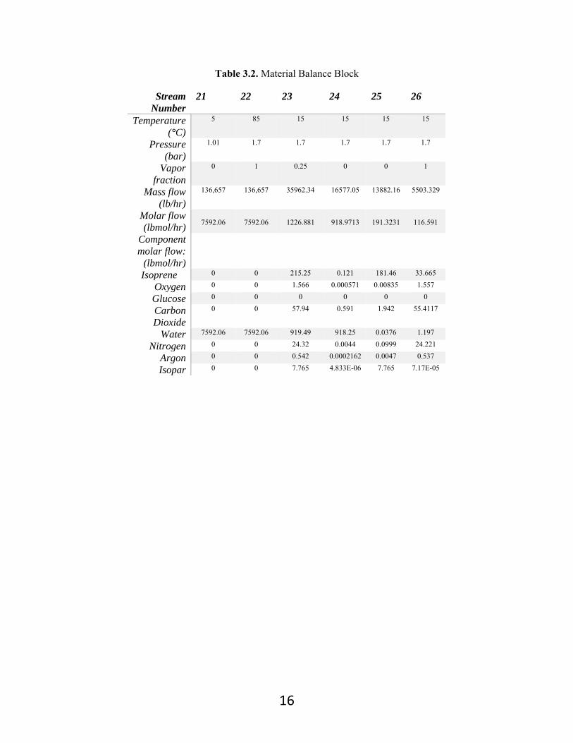
Table 3.2. Material Balance Block
Stream Number
21 22 23 24 25 26
Temperature (°C)
5 85 15 15 15 15
Pressure (bar)
1.01 1.7 1.7 1.7 1.7 1.7
Vapor fraction
0 1 0.25 0 0 1
Mass flow (lb/hr)
136,657 136,657 35962.34 16577.05 13882.16 5503.329
Molar flow (lbmol/hr)
7592.06
7592.06
1226.881
918.9713
191.3231
116.591
Component molar flow:
(lbmol/hr)
Isoprene 0 0 215.25 0.121 181.46 33.665
Oxygen 0 0 1.566 0.000571 0.00835 1.557
Glucose 0 0 0 0 0 0
Carbon Dioxide
0 0 57.94 0.591 1.942 55.4117
Water 7592.06 7592.06 919.49 918.25 0.0376 1.197
Nitrogen 0 0 24.32 0.0044 0.0999 24.221
Argon 0 0 0.542 0.0002162 0.0047 0.537
Isopar 0 0 7.765 4.833E-06 7.765 7.17E-05

17
Process Description
Figure 4. Block Flow Diagram for Isoprene Fermentation Process
5. Process overview:
The fermentation process is carried out using E.coli as a host platform. Once E.coli is
grown to the necessary concentrations, the isoprene production pathway is induced with
isopropyl-beta-D-1-thiogalactopyranoside (IPTG). Once induced, we assume that growth stops
and all glucose consumption by the microbe is directed towards the pathway. The off-gas from
the fermenter is taken off, carrying nearly all of the isoprene produced and sent to the absorption
column. In the absorption column, the fermenter off-gas is contacted with ISOPAR V, modeled
as a C13 paraffin solution in ASPEN, to bring the isoprene into solution. The remaining
incondensable gases are recycled back to the fermenter to bring the feed gas to 9.97% O2 to be
outside of the flammable levels for isoprene.
The isoprene-rich Isopar is piped to the stripper column where steam is injected to
vaporize the isoprene back into vapor phase for separation from Isopar. The steam stream
carrying the isoprene vapor enters a 3-phase flash at 15°C where more of the inert gases are
returned to the absorption column for further removal of isoprene. The two liquid phases exiting
Fermentation
34°C, 1.7bar
Absorption
34°C, 1.7bar
Stripper
34°C, 1.7bar
Flash 3
15°C, 1.7bar

18
the flash vessel are a water stream and a liquid isoprene stream containing some Isopar
contaminant. The isoprene stream is purified to 95% where it is stored at a quality grade that can
be used for polymerization. 0.02% wt% tert-butylcatechol is added to the isoprene to prevent
polymerization before usage.
2. Process Details:
The compressor (Block E-1) is used to bring the feed gas from the atmosphere up to 1.7
bars which is the pressure used in the fermentation process. This pressure was chosen because it
was the pressure tested at the bench-scale in the patents for the production of isoprene. Although
other pressures could most likely be used, there was no data to justify a use of a higher pressure.
Furthermore, a higher backpressure in the fermenters would allow for greater removal of
isoprene from the fermenter batch liquid rather than piping in gases at atmospheric pressure.
The mixer (Block E-6) at the beginning of the process is used to lower the feed gas O2
concentration down to 9.97%. During the patent review, it was discovered that the E.Coli was
consistently grown in reduced oxygen levels. Reduced oxygen helped drive carbon flux towards
the isoprene production pathway in E.Coli. 9.97% O2 in the feed gas was specifically chosen to
maximize the rate of production and reduce the risks of creating a flammable mix of vapors.
From the patent data, higher oxygen concentrations would lower the productivity of E.Coli. The
mixer combines air from the atmosphere as a source of O2 and the incondensable gases from the
absorption column (Block E-7) because using a N2 diluent source from an air liquefaction plant
or membranes is costly when only the oxygen concentration is the only important factor within
the feed gas as mentioned in the preliminary process synthesis.
The fermenters (Block E-5) are not well-represented in the flow diagram. The production
of isoprene calls for a continuous process for efficient purification to create the final product.
19
However, fermenters are typically not run continuously because of the increased risk of
contamination as time goes on; running fermenters in batch will allow for better response to
contaminated tanks as those cultures would need to be restarted. Our process proposes a 3-stage
step-up process from the shaker flasks produced in the laboratory to the full-scale fermentation
tanks used for isoprene production. From the 500mL shaker flasks grown from the initial stocks
of recombinant E.Coli, the pre-seed fermenters will grow the E.Coli up to 5L at 15g/L
concentration, taking 16 hours with exponential growth. The contents of the pre-seed fermenters
will be transferred into the seed fermenters to grow the E.Coli up to 88 m3 at 15g/L
concentration, taking another 26 hours with exponential growth. Once the E.Coli enters the
fermenters for production, each fermenter will be in growth phase for 8 hours to bring the
bacteria to 880 m3 at 15g/L where it will be ready to be induced using IPTG for directing glucose
consumption to the isoprene production pathway.
The process requires 4 production fermenters to produce a fixed amount of isoprene per
hour for continuous downstream processing assuming an 8 hour growth phase, 72 hour
fermentation phase, 10 hours for CIP/SIP, and 2 hours before the start of another batch to feed in
all the starting materials. However, this number is highly optimistic as we expect some batches
to become contaminated with other bacteria over the fermentation process, requiring a shutdown
of these fermenters. As such we propose to have an extra fermenter that will continually be in the
growth phase, ready to be induced for isoprene production in case any of the other fermenters
need to be taken off-line prematurely before the end of the batch cycle. Figure 5 shows a sample
Gantt chart of how the fermenters, seed fermenters, and pre-seed fermenters should be scheduled
to ensure a stable production rate. In this design, 5 fermenters, 3 seed fermenters, and 3 pre-seed
fermenters were used, but extra capacity for all fermenters should be considered if the

20
engineered E.Coli is weak, where there is a high probability of the cell culture dying out. At the
operating temperature and pressure of 34°C and 1.7 bar, isoprene is at a sufficiently dilute
concentration that all of the isoprene is vaporized into the off-gas.
Additionally, the seed and pre-seed fermenters will be designed to run at atmospheric
pressure. These fermenters will operate closely to a purely batch fermenter as all nutrients,
mainly glucose will be charged to the fermenters before the addition of E.Coli. However, to
promote the mass transfer of oxygen into the media, an arbitrary amount of filtered air will be
pumped through the fermenter so that oxygen can dissolve into the liquid as it is agitated.
Although 2.24 moles of oxygen is need for every mole of glucose consumed, any flow rate
higher than the stoichiometric amount can be used for equipment convenience. Once the E.Coli
is grown up to the amounts necessary for seeding the production fermenters, the liquid will be
pumped to a pressure of 1.7 bar before it is added.
Figure 5. Fermenter Scheduling
The off-gas from the fermenter is taken to the absorption column (Block E-7) where it is
contacted with Isopar v to bring the isoprene back into the liquid phase. The process is designed
so that nearly all of the isoprene is moved into the Isopar so that the only gases leaving the
21
absorption column are incondensable inerts and water vapor. The vapors leave the top of the
column at 34.8°C while the bottoms leave at 34.2°C
The isoprene-rich Isopar stream is injected into the stripping column (Block E-9) along
with saturated steam at 1.7 bar to vaporize the isoprene one more to separate the Isopar and
isoprene. The isoprene leaves the stripping column with the remaining steam and incondensable
gases at 107.8°C while the Isopar leaves at the bottom of the column with a second water phase
at 98.8°C. The bottoms from the stripping column which contains roughly a 50:50 split of water
and Isopar can be decanted to send the Isopar back to the absorption column so that the Isopar
does not need to be continuously replaced except for the small amount that is vaporized by the
steam and leaves the stripping column through the top.
The high temperature vapor stream carrying the isoprene is then cooled in a heat
exchanger (Block E-14) with chilled water to bring the temperature of the stream down to 15°C.
A 3-phase flash system (Block E-11) is used to separate the inerts, water, and isoprene/Isopar
into different streams. A distillation column was considered as an alternative to the flash system,
but the flash system was able to reach a high purity of isoprene without having to use additional
theoretical stages. Since a chilled water system is needed for the cooling the fermenters, the
benefits of adding a small amount of additional chilled water to the system for cooling the vapor
stream outweighs the costs associated with manufacturing and operating a distillation column.
The inerts that leave from the top of the flash is recycled back to the absorption to give a chance
for the Isopar to be separated again, while the water can be collected for use in the fermenters
again.

22
Energy Balance and Utility Requirements
This process requires a large amount of chilled water to cool the fermenters in
production. From the heat of formation calculations, the production of isoprene releases 1636
kJ/mol of glucose consumed. To meet our production needs, 451,193,000 kJ/hr of heat is
released by the 3 production fermenters. While it was desirable to meet the heat removal
requirements by using a combination of heat jackets and internal cooling loops, our calculations
showed that it would not be possible to fit enough tubes within the fermenter to allow for enough
surface area contact. Therefore, the fermenter contents will be pumped to an external heat
exchanger (Block E-12) to remove excess heat using chilled water. This will assume that any
increase in temperature experience before the heat exchanger will not affect the E.Coli. Since
chilled water cannot be heat beyond 15°C before returning it to the cooling tower, the chilled
water is a self-contained loop. Some additional chilled water will be needed for the vapor stream
leaving the stripping column to cool it down to 15°C before it enters the flash vessel for the
separation of isoprene from the other gases and water.
The compressed air introduced for the feed gas and the vapor stream leaving the stripping
column will also need cooling. Since the temperatures of this stream is 90.9°C cooling water can
be used as the cold stream for the heat exchanger cooling the air stream (Block E-3). For the pre-
flash heat exchanger (Block E-14), since the required temperature is 15°C, chilled water will
need to be used for this heat exchanger as well.
Many process requires the removal of heat because the process is constantly generating
heat through fermentation and steam is added at different places to aid with separation of our
product. As such, there is a high demand for cooling, while we do not see the need for much
heating within the process. Therefore, there is minimal benefits gained by attempting to integrate

23
the heat exchanger network, and so each heat exchanger is standalone. The following table
describes the cooling demands for various streams within the process.
Table 4. Cooling demands within process
Cooling Requirement
From Change in T To Change in T
4.512*108 KJ/hr Stream 9 34°C to 25°C Stream 10 5°C to 15°C 7.238*106 KJ/hr Stream 2 90.9°C to 34°C Stream 12 30°C to 80°C 2.075*107 KJ/hr Stream 20 98.4°C to 15°C Stream 21 5°C to 85°C

24
Equipment List and Unit Descriptions
1. Absorption Column.
The absorption column (Block E-7) was designed using a combination of hand
calculations and Aspen simulations. The number of actual stages that were required for the
separation was estimated using the Kremser equation. The calculations of the absorption factor
and number of actual stages are shown in the appendix.
Since the number of stages is an input for the Aspen flow sheet, the material balances for
the system were first solved by hand and the resulting flow rates were used for the Kremser
calculations. Also, Raoult’s law was used to calculate the K-value of isoprene assuming the feed
stream to the absorption was behaving ideally. Raoult’s law assumes an ideal mixture so the
Kremser calculations were based on this assumption. The number of actual stages was
determined to be 20 stages and sieve trays were used.
The diameter and height of the column were estimated using two methods: (1) using hand
calculations in Microsoft Excel, and (2) using Aspen simulations. After the number of stages was
computed using the Kremser method, the value was inputted into Aspen and the flow rates of
the absorption’s column feed stream, the column’s vapor product, and liquid product were
obtained from the simulation. These values were used to perform a flooding velocity calculation
which was then used to estimate the diameter and height of the column using the methods
outlined in Product and Process Design Principles by Seider, Seader, Lewin, and Widagdo.
The value for the diameter of the column was compared to the value that was obtained
from Aspen’s Tray Spacing Report. It’s important to note that Aspen’s estimate for the column
diameter was used for the calculations of the column’s capital and operating costs. The diameter

25
of the column was determined to be 34.81 ft with a height of 54 ft. Carbon Steel (SA-285 Grade
C) was chosen as the material for column due its price and availability and the sieve trays were
also made of Carbon Steel (SA-285 Grade C).
Using the methods outlined in Product and Process Design Principles by Seider, Seader,
Lewin, and Widagdo, the thickness and weight of the column were estimated, using the
operating pressure of 1.7 bar. The weight was then used to determine the vessel cost and the
purchase costs of the 20 sieve trays were also computed. The bare-module factor for the column
was determined to be 4.16 with a total bare-module cost of $18,608,456.
Since this is an absorption column, there is no reboiler or condenser. The only operating
cost stems from the use of Isopar as a solvent for isoprene. The operating costs were determined
to be $2,159,091.
When modeling the absorption column in ASPEN, the convergence of the column was
highly sensitive to the flow of Isopar. The Isopar flow had to be gradually reduced to find the
minimum flow rate that achieved our separation requirements. Carbon steel was used as the
construction material due to its low costs and mild operating conditions. Design calculation
initially done by hand can be found in the Appendix, and the specification sheet can be located
on page 38.
2. Stripping Column
The stripping column was designed using a similar method to that of the absorption
column. The stripping column (Block E-9) was designed using a combination of hand
calculations and Aspen simulations. The number of actual stages that were required for the
26
separation was estimated using the Kremser equation and the detailed calculations are shown in
the appendix.
As was mentioned in the previous section, the material balances for the system were first
solved by hand and the resulting flow rates were used for the Kremser equation calculations.
Raoult’s was used to calculate the K-value of isoprene assuming the feed stream to the
absorption was behaving ideally. The number of actual stages was determined to be 20 stages
and sieve trays were used.
The diameter and height of the column were estimated using two methods: (1) using hand
calculations in Microsoft Excel, and (2) using Aspen simulations. After the number of stages
were computed using the Kremser method, the number of stages was inputted into Aspen and the
flow rates of the stripping’s column feed stream, the column’s vapor product, and liquid product
were obtained from the simulation. These values were used to perform a flooding velocity
calculation which was then used to estimate the diameter and height of the column using the
methods outlined in Product and Process Design Principles by Seider, Seader, Lewin, and
Widagdo.
The value for the diameter of the column was compared to the value that was obtained
from Aspen’s Tray Spacing Report and the values that were generated by Aspen were used for
the estimates of the column’s capital and operating costs. The diameter of the column was
determined to be 39.5 ft with a height of 54 ft. Carbon Steel (SA-285 Grade C) was chosen as the
material for column due its price and availability and the sieve trays were also made of Carbon
Steel (SA-285 Grade C).
Using the methods outlined in Product and Process Design Principles by Seider, Seader,
Lewin, and Widagdo, the thickness and weight of the column were estimated. The weight was

27
then used to determine the vessel cost and the purchase cost of the 20 sieve trays was also
computed. The bare-module factor for the column was then determined to be 4.16 with a total
bare-module cost of $40,110,845.
Since this is a stripping column, there is no reboiler or condenser. The only operating cost
stems from the use of steam as a stripping agent. The operating cost was determined to be
$27,010,000 per year.
When modeling the stripping column in ASPEN, the convergence of the column was
highly sensitive to the flow of steam. The steam flow rate had to be gradually reduced to find the
minimum flow rate that achieved our separation requirements. Carbon steel was used as the
construction material due to its low costs and mild operating conditions. Design calculation
initially done by hand can be found in the Appendix, and the specification sheet can be located
on page 39.
3. Heat Exchangers (For the Fermenters)
The heat exchangers (Block E-12) were designed using hand calculations in Microsoft
Excel. The rate of heat removal was determined based on the heat of reaction and two methods
were used to estimate this quantity—the heats of formation and heats of combustion of the
products and reactants. It is important to note that this method inherently assumes that the heat of
metabolism of the E.coli is equal to the heat of the reaction involving the production of isoprene.
The heat of formation calculations resulted in a rate of heat removal of 4.512E+08 kJ/hr
which was equally distributed among three shell and tube heat exchangers. Initially, heating
jackets and cooling coils internal to the fermenters were considered but none of these methods
supplied a large enough heat transfer area for cooling. Therefore, the best option was to cool the

28
liquid contents of the fermenters externally using an external shell and tube heat exchanger. The
liquid contents were on the tube-side and the chilled water was on the shell side.
Since the fermentation temperature was 34 °C, the liquid contents were pumped out of
the tank at 34 °C and were cooled to 25 °C using the heat exchanger. The cooled liquid which
mainly consisted of water and dissolved gases was then pumped back into the fermenter. The
CPMX property set in Aspen was used to estimate the heat capacity at constant pressure for the
liquid contents of the fermenter and the molar flow rate was then computed using the specified
temperature difference, required rate of heat removal, and cp. The heat capacity of the liquid
contents was 0.075 kJ/mol-K with a molar flow rate of 493,550 lbmol/hr.
Chilled water at 5 °C was used for the cooling and the final temperature of the water
stream was determined using a ΔTmin of 19 °C. Therefore, the final temperature of the cooling
water was 15 °C and the mass flow rate of the the cooling water was calculated using the
specified temperature difference, required rate of heat removal, and cp. The required mass flow
rate of the cooling waster was 1,320,875 lbmol/hr.
Using the methods outlined in Product and Process Design Principles by Seider, Seader,
Lewin, and Widagdo, the size of the shell and tube heat exchanger was estimated. First, the log-
mean temperature difference was determined and the overall heat transfer coefficient (U) was
obtained using Table 18.5 in Product and Process Design Principles. The heat transfer area was
calculated using the required rate of heat removal, overall heat transfer coefficient, log-mean
temperature difference, and correction factor (FT). The overall heat transfer coefficient was
determined to be 225 BTU/°F-ft2-hr and the required heat transfer area was 18806 ft2.
A tube-side velocity of 17 ft/s was chosen and the number of tubes per pass was
computed assuming BWG tubing with an outer diameter of 0.75 in. and an inner diameter of

29
0.62 in. A tube length of 16 ft/s was selected and the number of tube passes was estimated using
the heat transfer area per tube. Next, a 1-in. square pitch was assumed and the inner diameter of
the shell was obtained using the tabulated data outlined in Product and Process Design
Principles. Also, the baffle spacing was also chosen to be half of the shell diameter. The number
of tubes was 991 tubes with 7 passes. A shell diameter of 170.32 in. was determined and the
baffle spacing was 102.19 in.
The capital cost of each heat exchanger was estimated using the methods listed in
Chapter 22 of Product and Process Design Principles. A fixed heat exchanger was assumed for
the calculations and Carbon Steel was chosen for the shell material due to its price and
availability. The shell diameter, required heat transfer area, and number of tubes were used to
estimate the bare-module factor and total mare-module cost of each exchanger. Since three heat
exchangers were required for our design, the total bare-module cost was determined to be
$2,065,920.14.
The only operating costs of the heat exchangers were the utility requirements for the
chilled water. The operating costs amounted to $14,438,188.99 assuming a price of $4 per
gigajoule of cooling.
Carbon steel was used as the construction material due to its low costs and mild operating
conditions. Design calculation initially done by hand can be found in the Appendix, and the
specification sheet can be located on page 40.
4. Heat Exchangers (For the Flash Vessel)
The heat exchanger (Block E-14) for the flash vessel’s feed stream (Block E-11) was
designed using a combination of our hand calculations in Microsoft Excel and Aspen
30
simulations. The vapor product that was leaving the stripping column had to be cooled to 15 °C
before it was fed to the flash vessel. The vapor phase was mainly composed of water vapor and
isoprene and the cooling was required to condense isoprene out of the vapor phase.
The required rate of heat removal was first estimated using our Aspen simulation. A
heater block was used to obtain the duty which was required to reduce the stripping column
vapor product’s temperature to 15 °C. A shell and tube heat exchanger with chilled water was
used for the cooling and the chilled water was on the tube-side and the vapor phase was on the
shell side. The final temperature of the chilled water stream was determined using a ΔTmin of
13.9 °C. Therefore, the final temperature of the chilled water was 85 °C and the mass flow rate
of the the chilled water was calculated using the specified temperature difference, required rate
of heat removal, and cp. The required mass flow rate of the cooling water was 7592 lbmol/hr.
Using the methods outlined in Product and Process Design Principles by Seider, Seader,
Lewin, and Widagdo, the size of the shell and tube heat exchanger was estimated. First, the log-
mean temperature difference was determined and the overall heat transfer coefficient (U) was
obtained using Table 18.5 in Product and Process Design Principles. The heat transfer area was
calculated using the required rate of heat removal, overall heat transfer coefficient, log-mean
temperature difference, and correction factor (FT). The overall heat transfer coefficient was
determined to be 60 BTU/°F-ft2-hr and the required heat transfer area was 15,368 ft2.
A tube-side velocity of 0.35 ft/s was chosen and the number of tubes per pass was
computed assuming BWG tubing with an outer diameter of 0.75 in. and an inner diameter of
0.62 in. A tube length of 16 ft/s was selected and the number of tube passes was estimated using
the heat transfer area per tube. Next, a 1-in. square pitch was assumed and the inner diameter of
the shell was obtained using the tabulated data outlined in Product and Process Design

31
Principles. Also, the baffle spacing was also chosen to be half of the shell diameter. The number
of tubes was 829 tubes with 7 passes. A shell diameter of 142.56 in. was determined and the
baffle spacing was 85.53 in.
The capital cost of the heat exchanger was estimated using the methods listed in Chapter
22 of Product and Process Design Principles. A fixed heat exchanger was assumed for the
calculations and Carbon Steel was chosen for the shell material due to its price and availability.
The shell diameter, required heat transfer area, and number of tubes were used to estimate the
bare-module factor and total mare-module cost of the exchanger. The total bare-module cost was
determined to be $337,772.49.
The only operating costs of the heat exchangers were the utility requirements for the
chilled water. The operating costs amounted to $663,941.78 assuming a price of $4 per gigajoule
of cooling.
Carbon steel was used as the construction material due to its low costs and mild operating
conditions. Design calculation initially done by hand can be found in the Appendix, and the
specification sheet can be located on page 41.
5. Heat Exchangers (For the Air Stream)
The heat exchanger for the air stream was designed using a similar method to that of the
fermenters’ heat exchangers. Hand calculations in Microsoft Excel were used to estimate the size
of the heat exchanger and the detailed calculations are shown in the appendix.
A fermenter pressure of 1.7 bar was outlined in U.S. Patent Application 20130164809
and this condition was used for our process. Since ambient air is at 25 °C and 1.01 bar, the air
first had to be compressed before it could be fed to the fermenter. Upon adiabatic compression,

32
the air stream’s temperature increased to 90.85 °C and it had to be cooled to 34 °C before it was
fed to the fermenter. The required rate of heat removal was calculated using the heat capacity of
air, the specified ΔT, and the mass flow rate of the air stream. The rate of heat removal was
7.238E+06 kJ/hr. Also, the air stream was on the shell-side and the cooling water was on the
tube-side of the heat exchanger.
Cooling water at 25 °C and 1.01 bar was used as the cold stream for the heat exchanger.
The final temperature of the water stream was determined using a ΔTmin of 10 °C. Therefore, the
final temperature of the cooling water was 80 °C and the molar flow rate of the the cooling water
was calculated using the specified temperature difference, required rate of heat removal, and Cp.
The required molar flow rate of the cooling water was 3260.07 lbmol/hr.
Using the methods outlined in Product and Process Design Principles by Seider, Seader,
Lewin, and Widagdo, the size of the shell and tube heat exchanger was estimated. First, the log-
mean temperature difference was determined and the overall heat transfer coefficient (U) was
obtained using Table 18.5 in Product and Process Design Principles. The heat transfer area was
calculated using the required rate of heat removal, overall heat transfer coefficient, log-mean
temperature difference, and correction factor (FT). The overall heat transfer coefficient was
determined to be 60 BTU/°F-ft2-hr and the required heat transfer area was 6414 ft2.
A tube-side velocity of 0.3 ft/s was chosen and the number of tubes per pass was
computed assuming BWG tubing with an outer diameter of 0.75 in. and an inner diameter of
0.62 in. A tube length of 16 ft/s was selected and the number of tube passes was estimated using
the heat transfer area per tube. Next, a 1-in. square pitch was assumed and the inner diameter of
the shell was obtained using the tabulated data outlined in Product and Process Design
Principles. Also, the baffle spacing was also chosen to be half of the shell diameter. The number
33
of tubes was 491 tubes with 5 passes. A shell diameter of 70.23 in. was determined and the
baffle spacing was 42.14 in.
The capital cost of the heat exchanger was estimated using the methods listed in Chapter
22 of Product and Process Design Principles. A fixed heat exchanger was assumed for the
calculations and Carbon Steel was chosen for the shell material due to its price and availability.
The shell diameter, required heat transfer area, and number of tubes were used to estimate the
bare-module factor and total mare-module cost of the exchanger. The total bare-module cost was
determined to be $115,220.99.
The only operating costs of the air stream’s heat exchanger was the utility requirements
for the cooling water. The operating costs amounted to $503,742.51 per year assuming a price of
$0.02 per m3 of cooling water.
Carbon steel was used as the construction material due to its low costs and mild operating
conditions. Design calculation initially done by hand can be found in the Appendix, and the
specification sheet can be located on page 42.
6. Fermenters
Since running the fermenters involves a batch process, the number of fermenters and their
size were determined by making sure that a constant flow rate of off-gas from the fermenters was
achieved, save for contaminations within the fermenters resulting in shutting down a tank. Thus,
for a 96 hour batch cycle, it was determined that the fermenter would be in the growth phase for
8 hours to reach 15g/L E.coli. Then, the fermenter would be induced and enter the fermentation
phase for 72 hours. After fermentation, the tanks would be cleaned for 10 hours with a CIP/SIP

34
cycle. There would be 4 hours of down time for any additional checks and then 2 hours to pipe in
the batch media to start the next cycle.
Based on the fact that isoprene had to be continuously produced, the water accumulation
from the isoprene production reaction, feed glucose solution, and the initial batch media itself
were considered. Since the necessary working volume after each 80 (8 growth + 72
fermentation) hour production cycle were known, Benz’s article on fermenter sizing, “Large-
Scale Microbial Production of Advanced Biofuels: How big can we go?” was used to interpolate
the specifications for the fermenter vessel and agitator. This process was repeated for the seed
fermenter as it was a large working volume. Finally, a rough quotation from Sartorius was
obtained for the pre-seed fermenter as it is a bench-scale fermenter (5L) and was already
commercially available. As such, the working volumes for the various size fermenters were
1850m3, 88m3, and 5L. Only the largest fermenters would be producing isoprene, and the seed
and pre-seed fermenters would only be used to grow E.coli to higher concentration needed for
the initial batch media for the 1850m3 tanks.
We were provided the information that 1 gram of glucose produces 0.56 grams of
biomass from Dr. Bockrath. Therefore, for our calculations of E.Coli biomass content within the
fermenters and the growth of E.Coli at the beginning of each batch cycle, we used the following
equation: C6H12O6 + 2.24 O2 = 4.1 CH1.2O0.5N0.2 + 1.90 CO2 + 2.31 H2O.
Carbon steel was used as the construction material due to its low costs and mild operating
conditions. The specification sheets for the various fermenter sizes can be located on pages 44-
46.
35
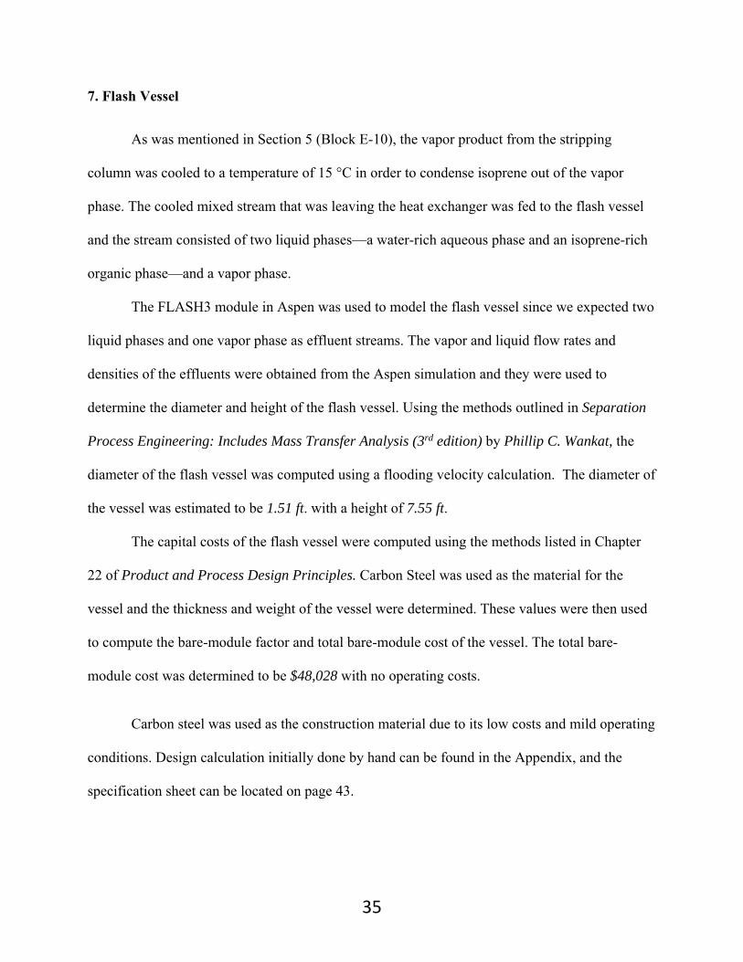
7. Flash Vessel
As was mentioned in Section 5 (Block E-10), the vapor product from the stripping
column was cooled to a temperature of 15 °C in order to condense isoprene out of the vapor
phase. The cooled mixed stream that was leaving the heat exchanger was fed to the flash vessel
and the stream consisted of two liquid phases—a water-rich aqueous phase and an isoprene-rich
organic phase—and a vapor phase.
The FLASH3 module in Aspen was used to model the flash vessel since we expected two
liquid phases and one vapor phase as effluent streams. The vapor and liquid flow rates and
densities of the effluents were obtained from the Aspen simulation and they were used to
determine the diameter and height of the flash vessel. Using the methods outlined in Separation
Process Engineering: Includes Mass Transfer Analysis (3rd edition) by Phillip C. Wankat, the
diameter of the flash vessel was computed using a flooding velocity calculation. The diameter of
the vessel was estimated to be 1.51 ft. with a height of 7.55 ft.
The capital costs of the flash vessel were computed using the methods listed in Chapter
22 of Product and Process Design Principles. Carbon Steel was used as the material for the
vessel and the thickness and weight of the vessel were determined. These values were then used
to compute the bare-module factor and total bare-module cost of the vessel. The total bare-
module cost was determined to be $48,028 with no operating costs.
Carbon steel was used as the construction material due to its low costs and mild operating
conditions. Design calculation initially done by hand can be found in the Appendix, and the
specification sheet can be located on page 43.
36
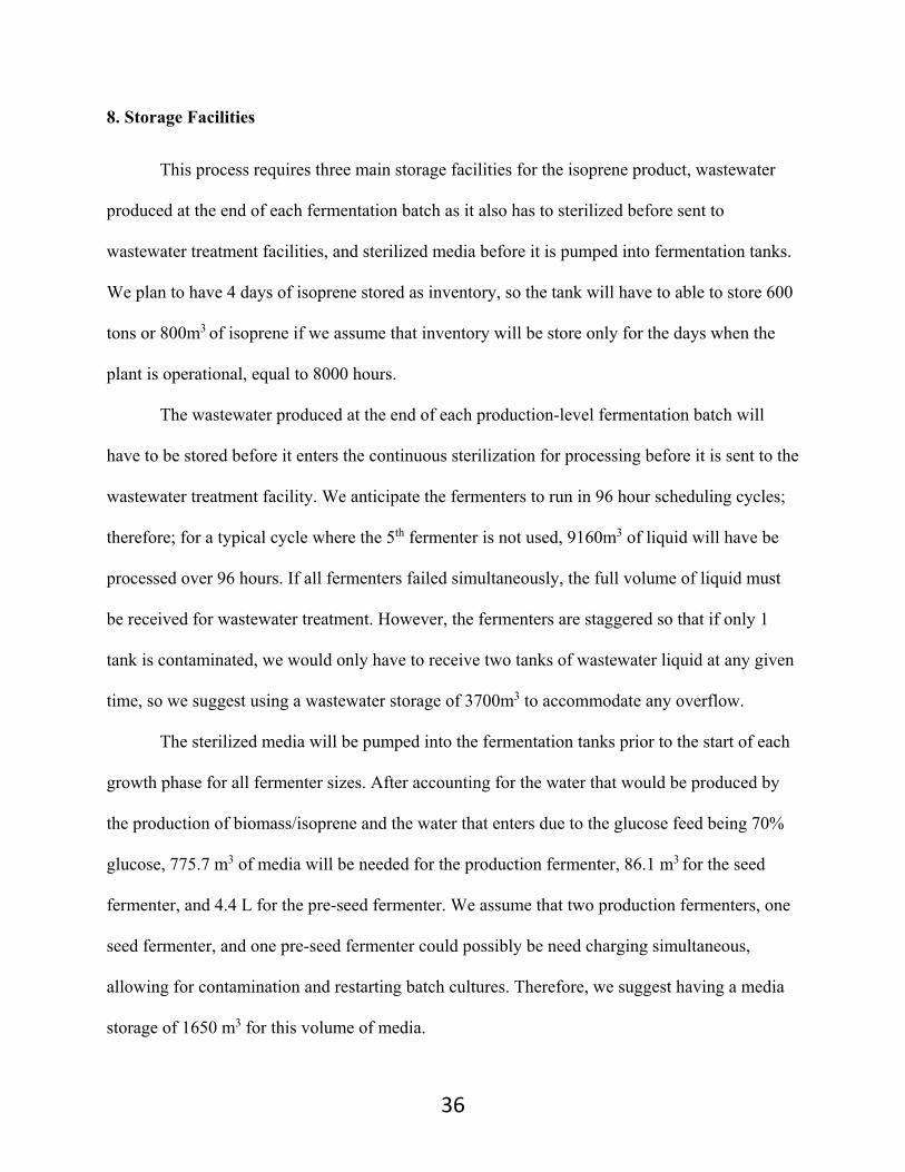
8. Storage Facilities
This process requires three main storage facilities for the isoprene product, wastewater
produced at the end of each fermentation batch as it also has to sterilized before sent to
wastewater treatment facilities, and sterilized media before it is pumped into fermentation tanks.
We plan to have 4 days of isoprene stored as inventory, so the tank will have to able to store 600
tons or 800m3 of isoprene if we assume that inventory will be store only for the days when the
plant is operational, equal to 8000 hours.
The wastewater produced at the end of each production-level fermentation batch will
have to be stored before it enters the continuous sterilization for processing before it is sent to the
wastewater treatment facility. We anticipate the fermenters to run in 96 hour scheduling cycles;
therefore; for a typical cycle where the 5th fermenter is not used, 9160m3 of liquid will have be
processed over 96 hours. If all fermenters failed simultaneously, the full volume of liquid must
be received for wastewater treatment. However, the fermenters are staggered so that if only 1
tank is contaminated, we would only have to receive two tanks of wastewater liquid at any given
time, so we suggest using a wastewater storage of 3700m3 to accommodate any overflow.
The sterilized media will be pumped into the fermentation tanks prior to the start of each
growth phase for all fermenter sizes. After accounting for the water that would be produced by
the production of biomass/isoprene and the water that enters due to the glucose feed being 70%
glucose, 775.7 m3 of media will be needed for the production fermenter, 86.1 m3 for the seed
fermenter, and 4.4 L for the pre-seed fermenter. We assume that two production fermenters, one
seed fermenter, and one pre-seed fermenter could possibly be need charging simultaneous,
allowing for contamination and restarting batch cultures. Therefore, we suggest having a media
storage of 1650 m3 for this volume of media.

37
The following table shows the equipment list summary in a concise table.
Table 5. Equipment List
Block
Number
Unit Type Unit
Number
Material of
Construction
Size
(h/l x w)
Operating T
and P
E-7 Absorption
Column
1 Carbon Steel 54ft x 34.8ft 34.2-34.8°C,
1.7 bar
E-9 Stripping Column 1 Carbon Steel 54ft x 39.5ft 98.8-107.8°C, 1.7
bar
E-12 Fermenter Heat
Exchanger
3 Carbon Steel 16ft x 170in 1.7 bar
E-3 Air Heat
Exchanger
1 Carbon Steel 16ft x 53.7in 1.7 bar
E-14 Pre-flash Heat
Exchanger
1 Carbon Steel 16ft x 53.7in 1.7 bar
E-11 Flash Vessel 1 Carbon Steel 7.55ft x 1.51ft 15°C, 1.7 bar
E-5 Fermenter 5 Carbon Steel 33.2m x 9.9m 34°C, 1.7 bar
E-5 Seed Fermenter 3 Carbon Steel 12.2m x 3.6m 34°C, 1 bar
E-5 Pre-seed Fermenter 3 Carbon Steel 1.3m x 0.7m 34°C, 1 bar
N/A Isoprene Storage
Tank
1 Carbon Steel 800m3 25°C, 1 bar
N/A Wastewater
Storage Tank
1 Carbon Steel 3700m3 25°C, 1.7 bar
N/A Media Storage
Tank
1 Carbon Steel 1650 m3 25°C, 1.7 bar

38
Specification Sheets
Figure 6. Specification sheet for absorption column
Absorption Column
Identification: Item Absorption Column Item No. E-7 No. required 1
Date: 4 April 2016
By: Phillip Taylor
Function: Separate isoprene from water vapor, CO2, Argon, and other non-condensables.
Operation: Continuous
Materials handled: Quantity (lbmol/hr): Composition (lbmol/hr):
Isoprene Oxygen Glucose
Carbon Dioxide Water
Nitrogen Argon Isopar
Temperature (°C)
Feed 1 21,597
185.5 697.5
0 4244.81 685.74
15596.34 186.34 0.864
34
Feed 2 18,298.37
0 0 0 0 0 0 0
18,298.37
34
Bottoms 18616.27
215.25 1.566
0 57.944 19.089 24.324 0.542
18297.55
34.85
Vapor 21395.76
3.90 697.49
0 4242.27 667.85
15596.23 186.33 1.677
34.18
Feed 3 116.591
33.665 1.557
0 55.4117
1.197 24.221 0.537
7.17E-05
15
Design Data: Number of trays: 20 Pressure: 1.7 bar Functional Height: 54 ft Material of construction: Carbon steel Recommended inside diameter: 34.81 ft Tray efficiency: 0.70 Feed 1 stage: 20 Feed 2 stage: 1 Feed 3 stage: 7
Tray spacing: 24 in.
Utilities: Controls: Tolerances: Comments and drawings: See Process Flow Sheet and Appendix.

39
Figure 7. Specification Sheet for Stripping Column
Stripping Column
Identification: Item Stripping Column Item No. E-9 No. required 1
Date: 4 April 2016
By: Phillip Taylor
Function: Separate isoprene from Isopar, water vapor, CO2, and other non-condensables.
Operation: Continuous
Materials handled: Quantity (lbmol/hr): Composition (lbmol/hr):
Isoprene Oxygen Glucose
Carbon Dioxide Water
Nitrogen Argon Isopar
Temperature (°C)
Feed 1 18616.27
215.25 1.566
0 57.944 19.089 24.324 0.542
18297.55
34.85
Feed 2 18739.29
0 0 0 0
18739.29 0 0 0
115.61
Bottoms 36128.68
3.83E-18 5.97E-48
0 1.93E-29 17838.89 3.91E-50 3.62E-50 18289.79
107.75
Vapor 1226.881
215.25 1.566
0 57.94
919.49 24.32 0.542 7.765
98.39
Design Data: Number of trays: 20 Pressure: 1.7 bar Functional Height: 54 ft Material of construction: Carbon steel Recommended inside diameter: 39.53 ft Tray efficiency: 0.70 Feed 1 stage: 1 Feed 2 stage: 20
Tray spacing: 24 in.
Utilities: Controls: Tolerances: Comments and drawings: See Process Flow Sheet and Appendix.

40
Figure 8. Specification sheet for shell and tube heat exchanger for fermenters
Fermenter Shell and Tube Heat Exchanger
Identification: Item Heat Exchanger Item No. E-12 No. required 3
Date: 4 April 2016
By: Phillip Taylor
Function: Maintain a fermentation temperature of 34 °C.
Operation: Continuous
Materials handled: Quantity (lbmol/hr): Composition (lbmol/hr):
Isoprene Oxygen Glucose
Carbon Dioxide Water
Nitrogen Argon Isopar
Temperature (°C)
Hot In 493,550
1.46 0.54
0 78.78
493,462.97 6.29 0.16 0.01
34
Cold In 1,320,875.3
0 0 0 0
1,320,875.30 0 0
5
Hot Out 493,550
1.46 0.54
0 78.78
493,462.97 6.29 0.16 0.01
25
Cold Out 1,320,875.3
0 0 0 0
1,320,875.30 0 0
15
Design Data: Heat Transfer Area: 18805.64 ft2 Type of tubing: BWG O.D of tubing: 0.75 in. I.D of tubing: 0.62 in. Material of construction for shell: Carbon steel Number of tubes per pass: 991 Length of tube: 16 ft Number of passes 7 I.D of shell: 170.32 in.
Baffle spacing: 102.19 in.
Utilities: 1,320,875 lbmol/hr of chilled water at 5 °C and 1.01 bar. Controls: Tolerances: Comments and drawings: See Process Flow Sheet and Appendix.

41
Figure 9. Specification sheet for shell and tube heat exchanger before entering flash vessel
Pre-Flash Shell and Tube Heat Exchanger
Identification: Item Heat Exchanger Item No. E-14 No. required 1
Date: 4 April 2016
By: Phillip Taylor
Function: Maintain a flash temperature of 15 °C.
Operation: Continuous
Materials handled: Quantity (lbmol/hr): Composition (lbmol/hr):
Isoprene Oxygen Glucose
Carbon Dioxide Water
Nitrogen Argon Isopar
Temperature (°C)
Hot In 1226.881
215.25 1.566
0 57.94
919.49 24.32 0.542 7.765
98.39
Cold In 7592.06
0 0 0
7592.06 0 0 0 0
5
Hot Out 1226.881
215.25 1.566
0 57.94
919.49 24.32 0.542 7.765
15
Cold Out 7592.06
0 0 0
7592.06 0 0 0 0
85
Design Data: Heat Transfer Area: 15,368.2 ft2 Type of tubing: BWG O.D of tubing: 0.75 in. I.D of tubing: 0.62 in. Material of construction for shell: Carbon steel Number of tubes per pass: 829 Length of tube: 16 ft Number of passes 7 I.D of shell: 53.66 in.
Baffle spacing: 32.20 in.
Utilities: 7585.63 lbmol/hr of cooling water at 15 °C and 1.01 bar. Controls: Tolerances: Comments and drawings: See Process Flow Sheet and Appendix.

42
Figure 10. Specification sheet for shell and tube heat exchanger for feed gas
Air Shell and Tube Heat Exchanger
Identification: Item Heat Exchanger Item No. E-3 No. required 1
Date: 4 April 2016
By: Phillip Taylor
Function: Maintain an air temperature of 34 °C.
Operation: Continuous
Materials handled: Quantity (lbmol/hr): Composition (lbmol/hr):
Isoprene Oxygen Glucose
Carbon Dioxide Water
Nitrogen Argon Isopar
Temperature (°C)
Hot In 9686.67
0 2029.36
0 2.62
0 7564.32 90.3766
0
90.85
Cold In 3260.07
0 0 0 0
3260.07 0 0 0
30
Hot Out 9686.67
0 2029.36
0 2.62
0 7564.32 90.3766
0
34
Cold Out 3260.07
0 0 0 0
3260.07 0 0 0
80
Design Data: Heat Transfer Area: 4,363.56 ft2 Type of tubing: BWG O.D of tubing: 0.75 in. I.D of tubing: 0.62 in. Material of construction for shell: Carbon steel Number of tubes per pass: 312 Length of tube: 16 ft Number of passes 5 I.D of shell: 53.66 in.
Baffle spacing: 32.20 in.
Utilities: 9686.67 lbmol/hr of cooling water at 15 °C and 1.01 bar. Controls: Tolerances: Comments and drawings: See Process Flow Sheet and Appendix.

43
Figure 11. Specification sheet for 3 stream flash vessel
3 Stream Flash Vessel
Identification: Item Flash Vessel Item No. E-11 No. required 1
Date: 4 April 2016
By: Phillip Taylor
Function: Flash the stream leaving the stripping column to separate isoprene
Operation: Continuous
Materials handled: Quantity (lbmol/hr): Composition (lbmol/hr):
Isoprene Oxygen Glucose
Carbon Dioxide Water
Nitrogen Argon Isopar
Temperature (°C)
Inlet 1226.881
215.25 1.566
0 57.94
919.49 24.32 0.542 7.765
15
Vapor 116.591
33.665 1.557
0 55.4117
1.197 24.221 0.537
7.17E-05
15
Liquid 1 191.3231
181.46 0.00835
0 1.942
0.0376 0.0999 0.0047 7.765
15
Liquid 2 918.9713
0.121 0.000571
0 0.591
918.25 0.0044
0.0002162 4.833E-06
15
Design Data: Pressure: 1.7 bar Height: 7.55 ft Diameter: 1.51 ft Material of construction: Carbon steel
Utilities: Controls: Tolerances: Comments and drawings: See Process Flow Sheet and Appendix.

44
Figure 12. Specification sheet for fermenter
Fermenters
Identification: Item Fermenter Item No. E-3 No. required 5
Date: 4 April 2016
By: Yuta Inaba
Function: Ferment E.Coli on glucose to produce isoprene
Operation: Batch
Materials handled: Quantity (lbmol/hr): Composition (lbmol/hr ):
Isoprene Oxygen Glucose
Carbon Dioxide Water
Nitrogen Argon Isopar
Temperature (°C)
Feed Gas 6901.83
0.67 796.2
0 729.1 114.6
5198.8 62.1 0.287
34
Glucose Feed 873.77
0 0
165.3 0
708.5 0 0 0
34
Off-gas 7199
61.8 232.5
0 1414.9 228.58
5198.78 62.11 0.288
34
Design Data: Temperature: 34°C Pressure: 1.7 bar Working Volume: 1850 m3
Diameter: 9.9 m Tank Height: 33.2 m Maximum Liquid Level: 24.7 m Agitator Motor Size: 4770 kW Brake Compressor Size: 8385kW Impeller Size: 2.5m x4
Shaft Diameter: 362mm Oxygen Transfer Rate: 200 mmol/L-hr
Utilities: Controls: Tolerances: Comments and drawings: See Process Flow Sheet and Appendix. Connected directly to external heat exchanger
Liquid Accumulation (lbmol) 223511
0.287 0.105
0 15.4
223494 1.23
0.031 0.003
34

45
Figure 13. Specification sheet for seed fermenter
Seed Fermenters
Identification: Item Fermenter Item No. E-3 No. required 3
Date: 4 April 2016
By: Yuta Inaba
Function: Grow E.Coli to necessary concentration for the fermenter.
Operation: Batch
Materials handled: Quantity (lbmol): Composition (lbmol):
Isoprene Oxygen Glucose
Carbon Dioxide Water
Nitrogen Argon Isopar
Temperature (°C)
Batch Media 10696
0 0
28.83 0
10667 0 0 0
34
Design Data: Temperature: 34°C Pressure: 1.7 bar Working Volume: 88 m3
Diameter: 3.6 m Tank Height: 12.2 m Maximum Liquid Level: 9.0 m Agitator Motor Size: 510 kW Brake Compressor Size: 385kW Impeller Size: 1.3m x4
Shaft Diameter: 138 mm Oxygen Transfer Rate: 200 mmol/L-hr
Utilities: Controls: Tolerances: Comments and drawings: See Process Flow Sheet and Appendix.

46
Figure 14. Specification sheet for pre-seed fermenter
Pre-seed Fermenters
Identification: Item Fermenter Item No. E-3 No. required 3
Date: 4 April 2016
By: Yuta Inaba
Function: Grow E.Coli to necessary concentration for the seed fermenter
Operation: Batch
Materials handled: Quantity (lbmol): Composition (lbmol):
Isoprene Oxygen Glucose
Carbon Dioxide Water
Nitrogen Argon Isopar
Temperature (°C)
Batch Media 0.609
0 0
0.001 0
0.608 0 0 0
34
Design Data: Temperature: 34°C Pressure: 1.7 bar Working Volume: 5 L
Diameter: 0.7 m Tank Height: 1.3 m Maximum Liquid Level: 0.97 m Agitator Motor Size: 0.5 kW Brake Compressor Size: N/A Impeller Size: 0.4m x6
Shaft Diameter: 138 mm Oxygen Transfer Rate: 200 mmol/L-hr
Utilities: Controls: Tolerances: Comments and drawings: See Process Flow Sheet and Appendix. Specifications obtained from Sartorius.

47
Equipment Cost Summary
The fermenters constitute the highest equipment cost because of the numerous
components required in their construction (vessel costs/agitators/etc.). The absorption and
stripping column are the next highest costs, partially because of their complexity in design. The
other equipment costs are much lower compared to these three parts of the plant design.
These prices were determined using the tabulated costs in Product and Process Design
Principles by Seider, Seader, Lewin, and Widagdo for the various pieces of equipment.
Table 6. Equipment cost summary
Equipment Block Number Purchase Cost
Absorption Column E-7 $4,473,187
Stripping Column E-9 $9,642,030
Fermenters/Agitator (all) E-5 $47,794,800
Heat Exchangers (Fermenters) E-12 $641,590
Compressor E-1 $1,228,888
Heat Exchanger (Air Stream) E-3 $35,783
Flash Vessel E-11 $11,545
Heat Exchanger (Pre-flash) E-14 $48,103
The purchase costs of the equipment were estimated using the methods outlined in
Product and Process Design Principles by Seider, Seader, Lewin, and Widagdo assuming a CE
price index of 500. The detailed calculations are shown in the appendix.

48
Fixed-capital Investment Summary
The fixed-capital investment takes the purchase cost of each equipment piece and
incorporates the costs of installation including direct field materials and labor, freight, overhead,
and contract expenses. This adjustment in costs is lumped as a bare module factor which is a
multiplicative factor for the purchase costs shown in the previous section. The total bare module
cost for this process is $219,177,000.
Figure 15. Bare Module Costs for equipment

49
Operating Cost
The operating cost of this plant includes fixed costs and variable costs. As can be seen
below in Table 5, the raw materials and utilities are a significant proportion of the variable costs.
Unless the cost of glucose, the major material input, is reduced, the costs incurred to produce
isoprene is not favorable for this process. To produce 50,000 tons of isoprene per year, the
process incurs $456 million in variable costs each year. We assumed that we would be directly
receiving 70% glucose from a company like Cargill which has corn mills located in Iowa, so that
we will not to have to pay transportation costs for our high consumption rate of glucose.
Figure 16 shows the raw materials needed for the isoprene process. Since the
fermentation batch media requires many minor chemicals to be dissolved in, these prices are
accounted by taking the weighted average weight and price for these compounds. Figure 17 then
shows the utility costs when assuming that we would be getting our utilities provided by a nearby
plant.
Figure 16. Raw materials variable costs

50
Figure 17. Utility variable costs for isoprene
Figure 18 shows our total variable costs when general expenses are combined with the
raw materials and utilities costs for production. Raw materials constitute most of our variable
cost as the price of glucose is a major factor driving up the costs for this process. Our total
variable cost at full capacity is $456 million.
Figure 18. Estimate of total variable costs when producing 50,000 tons of isoprene

51
Table 6 lists the fixed costs of the plant. The overhead is calculated in accordance with
the guidelines from Product and Process Design Principles. These expenses are required to
operate the plant as they include operator salaries, maintenance, and general business
management. The total overhead leads to an annual expense of $1.7 million.
Table 6. Fixed overhead costs per year
Fixed Costs Operations Direct Wages and Benefits $ 416,000 Direct Salaries and Benefits $ 62,400 Operating Supplies and Services $ 24,960 Technical Assistance to Manufacturing $ 300,000 Control Laboratory $ 325,000 Total Operations $ 1,128,360 Maintenance Wages and Benefits $ 151,913 Salaries and Benefits $ 37,978 Materials and Services $ 151,913 Maintenance Overhead $ 7,596 Total Maintenance $ 349,399 Operating Overhead General Plant Overhead: $ 47,449 Mechanical Department Services: $ 16,039 Employee Relations Department: $ 39,429 Business Services: $ 49,454 Total Operating Overhead $ 152,370 Property Taxes and Insurance Property Taxes and Insurance: $ 67,517 Other Annual Expenses Rental Fees (Office and Laboratory Space): $ - Licensing Fees: $ -

52
Miscellaneous: $ - Total Other Annual Expenses $ - Total Fixed Costs $ 1,697,646
Other Considerations
1. Safety
Isoprene is a flammable liquid and it is the only major safety hazard for our process.
Isoprene must be stored and used with adequate ventilation. Its containers should be kept closed
and it should be stored only where temperatures will not exceed 125 °F (52 °C). Full and empty
containers of isoprene should be stored separately and a first-in, first-out inventory system
should be used to prevent the storage of full containers for long periods.
There are several precautions which must be taken when handling isoprene. Inhalation
and contact with eyes, skin, and clothing should be avoided. Isoprene should be kept away from
heat, sparks, and open flames and only spark-proof tools and explosion-proof equipment should
be used. Safety showers and eye-baths should be readily available and you should not eat, drink,
or smoke in areas where isoprene is stored or used. Also, after working with this material, you
should wash your face and hands thoroughly with soap and water before eating, drinking,
smoking, applying cosmetics, or using the toilet. Prolonged and repeated exposure to isoprene
should also be avoided.
Using the MSDS, the flammability limits for isoprene were obtained:
Lower flammability limit (in air): 1.5%
Upper flammability limit (in air): 9.7%

53
None of the streams in our system had an isoprene concentration that fell within the
flammability limit therefore fires and explosions should not be an issue, but any changes in
isoprene concentration during startup should be monitored to remain outside this range.
2. HAZOP Analysis
Since, a P&ID diagram does not exist for this process, the HAZOP analysis will instead
be focused around the primary sections of the system: that is the fermentor section, the absorber
and stripping section, and the storage of isoprene . The best method to prevent any kind incident
and to ensure personnel safety is the use of PPE ( Personal Protective Equipment).The purpose of
using PPE is to protect against a majority of the hazards at the plant. Although it is subject to
change depending on the materials or environment, the primary PPE that the operator should
have on hand should be a hard hat, protective goggles, earplugs, hard toes shoes, gloves, and
flame retardant clothing. This equipment is used to protect against any hazardous material that
can contact the body, flash fires, and noise pollution that is produced due to the industrial sized
equipment.
Fermenter Section:
At the fermenters, the main safety concerns that could lead to accidents or operating
problems is the leakage of off gas at the outlet. This would create an asphyxiation hazard for
operators at the plant. Since the offgas contains a small amount of oxygen and isoprene which
can be toxic when inhaled in large amounts, proper asphyxiation safety procedures should be
followed for any work done in that area. The main causes of asphyxiation hazards are failure to
detect an oxygen deficient atmosphere in and around confined spaces and inadequately preparing
for recognition and rescue. One primary area of concern is that there is only one operator at the

54
plant. Should there be an incident where he finds himself in a potential low oxygen atmosphere,
there will be nobody to help him. In order to prevent an incident like this from happening in the
first place, a few safety measures should be implemented. For example, a continuous monitoring
of oxygen deficient environments around equipment that is dealing with the off gas or isoprene.
Warning systems with alarms could be implemented in order to alert the operator that an oxygen
deficient environment has occurred near the equipment. Furthermore, the operator should carry a
personal monitor that measures oxygen concentration in the air so that should he or she enter an
area that presents a potential asphyxiation hazard, they can evacuate the area with caution and
wait for further assistance.
Absorber and Stripping Column Section:
At the absorber column one safety concern is the handling of ISOPAR V. There are fire
and explosion risks associated with static accumulation and discharge. In order to prevent this,
the transfer system of the isopar should be effectively bound or ground in accordance with the
National Fire Protection Association publications. The containers should be kept closed when
not in use and should not be stored near heat, sparks, flame or strong oxidants. Although an
asphyxiation hazard is also present here, it only applies towards the top of the column if any
maintenance is being done.
At the stripper, the same safety concerns exist as for the absorber. However, one
important additional concern is the use of steam. Since the steam is coming in at 115 degrees
Celsius, it presents a burning hazard if the operator makes contact with the piping. In order to
prevent this, any piping that is transporting steam needs to be insulated for heat. Not only does
this prevent the loss of heat but it also help ensure safe handling of the steam piping. This also
applies to the liquid stream leaving the stripper which is leaving at a temperature of 107 degrees.

55
For both the stripper and the absorber there are structural safety concerns due to the size
of the equipment. These include vibrations, corrosion, and overheating or overpressurization.
These can be solved with proper maintenance and management of the equipment so that any of
these problems can be quickly identified and the proper steps can be taken to ensure they are
fixed.
Isoprene Storage:
The purified isoprene at the end of the process will be stored in a storage tank. Although
it is being stored as a liquid, the potential for the isoprene vaporizing towards the top of the
stored liquid exists. This could cause a pressure hazard that may affect the integrity of the tank.
In order to decrease this concern, a pressure relief system should be installed on the tank along
with a vapor recovery system since the isoprene gas cannot be released to the environment due to
EPA regulations.
3. Startup
Since the recycle loop is required for the dilution of air to an oxygen concentration of
9.97 vol%, a diluent has to be used during the startup of the process. Based on the
recommendations of one of our industrial consultants, Dr. Richard Bockrath, methane gas will be
burned and used as a diluent for the fermenter’s air stream during startup.
It is important to note that the products of the combustion of methane include carbon
dioxide and water vapor. Since a considerable amount of CO2 will be pumped into the system
during startup, this also means that the concentration of CO2 that enters the fermenter will also
be quite large. CO2 is inhibitory to the growth of the E.coli so the initial production rate of
isoprene might be below the predicted rate of 2.2 g/hr-L.

56
4. Environmental Concerns and Waste Removal
Wastewater treatment and disposal is one important area of consideration. As can be seen
from the reaction mechanism, one of the primary byproducts from the isoprene reaction is water.
Since there is an abundance of water produced there needs to be a way to treat and reuse it. The
primary impurity in the water would be any dead E.coli that is left after the fermentation process
is complete. This treatment process would be a two-step process. Primary treatment would
include filtration of the water with coarse and fine screens and a hydrocyclone in order to remove
and solids and E.Coli from the water. Secondary treatment would be a process in which we
evaporate the water in four stages to recover some water to be inputted back to the process. The
steam would be filtered using a scrubber. The initial three stages would be sent back as clean
water and one would be sent to the waste treatment plant.

57
Profitability Analysis
This process is highly unprofitable due to the high operating expenses needed to produce
isoprene, disregarding any capital investments needed for equipment. Due to reaction
stoichiometry in the E.Coli, 10.21 lb of glucose is need per pound of isoprene. Thus, to even
begin making positive revenue for this process, glucose prices will either have to drop to
$0.077/lb or isoprene prices will have to increase to $4.084/lb. While it is difficult to foresee
glucose prices falling in the future, it is possible that isoprene prices could return to prices of
around $1.50/lb. However, the current metabolic pathway does not effectively convert glucose
into isoprene, resulting in a low process efficiencies.
Some profitability measures are listed below, but calculations are not required to show
that there will be a high deficit from the input costs for this process. Because of the imbalance
between the cash obtained from selling the isoprene to the expenses made for the raw materials,
the IRR and ROI predicted for this process are unreasonably large. Without a lower input cost of
glucose or a higher price of isoprene, this process will begin with a deficit, and this deficit will
continue to grow as the fixed costs for purchasing equipment and other administrative costs are
added. Figure 19 shows these values for completeness, but are not very useful under the
assumptions we made for various prices.

58
Figure 19. Some key profitability measures for this process.
Additionally, we assumed a 5 year accelerated depreciation schedule in hopes of reducing
some of our initial losses, but even with this generous assumption, our cash flows are highly
negative year after year. Figure 20 shows the depreciation schedule and Figure 21 shows our
yearly cash flow summary assuming that this plant will be operational for 15 years.
Figure 20. 5 Year accelerated depreciation schedule used for the process.

59
Figure 21. Cash flow projection using a 15 year timeline
A very generous sensitivity analysis was calculating, assuming that the isoprene prices
could be volatile in the upcoming years, causing the price to increase. Figure 22 shows this
sensitivity analysis showing the effects of different isoprene prices and variable costs, but as
stated before, the analysis is not very helpful when the process’s key input component of glucose
costs more than the isoprene.
Figure 22. Sensitivity analysis on price of isoprene and variable costs

60
Conclusions and Recommendation
The production of isoprene via the fermentation of glucose is a novel yet unprofitable
venture. Based on the results of our analysis, we have concluded that our design simply does not
have a competitive advantage. The price of isoprene is too low when compared to the costs of
raw materials and the chemical pathway for the production of isoprene is also highly exothermic.
The large rate of heat removal for the fermenters resulted in astronomically large utility
requirements for chilled water. Another issue is that the fermentation has to be operated at a
pressure of 1.7 bar. The electricity costs due to the use of a compressor were considerable and
large amounts of Isopar and steam were required for the absorption and stripping columns.
As for any plant design, there is certainly room for improvement regarding our current
design. One method which would decrease the raw material costs is that stream 19—i.e. the
liquid product leaving the stripping column—could be recycled back to the absorption column.
The liquid product leaving the stripping column is rich in Isopar and the reuse of the solvent
would significantly decrease the plant’s operating costs. Another issue is that the isoprene
product is obtained as a liquid (stream 25) with a purity of approximately 95%. The purity of the
isoprene product can be increased to 99% by adding a second flash vessel which would separate
the isoprene from the remaining Isopar that is present in stream 25.
A third recommendation is that the isoprene that’s lost at the end of every fermentation
batch can be recycled. Isoprene is immiscible with water so the liquid contents of the fermenter
is essentially a two-phase system—an isoprene-rich phase and an aqueous phase. A decanter can
be used to separate the two immiscible layers and the isoprene layer could be obtained with a

61
fairly high purity. Based on our estimates, 0.85 lbmol of isoprene are being lost per fermentation
batch which amounts to a total of 95.5 lbmol of isoprene which can be recovered per year.

62
Acknowledgments
Thanks to Dr. Sue Ann Bidstrup-Allen, Dr. Richard Bockrath, and all of our other industrial
advisors for their assistance and support during the design of this process. Special thanks are also sent to
Professor Leonard Fabiano for his guidance regarding the design of our Aspen flow sheet and his efforts
to contact the AspenTech support team.
Bibliography
1. Chotani, G. K., et al. , Production of Isoprene under Reduced Oxygen Inlet Levels, U.S. Patent
Application 20130164809 A1 (2013).
2. Feher et al., Purification of Isoprene from renewable resources, U.S. Patent Application 2011/0178261
A1 (2011).
3. Chotani et al., Reduction of Carbon Dioxide Emission during Isoprene Production by Fermentation,
U.S. Patent 8,470,581 (2013).
4. Seider, Warren D., J. D. Seader, Daniel R. Lewin, and Warren D. Seider. Product and Process Design
Principles: Synthesis, Analysis, and Evaluation. New York: Wiley, 2004. Print.
5. Benz, Gregory T. "Large Scale Microbial Production of Advanced Biofuels: How Big Can We
Go?" Biofuels Digest. Benz Technology International, Inc. Web. 05 Apr. 2016.
6. Isoprene; MSDS Catalog Code SLI1204 [Online]; Science Lab.com: Houston, Texas,
http://www.sciencelab.com/msds.php?msdsId=9924409 (accessed April 5, 2016).
7. Yaws, Carl L. Chemical Properties Handbook. McGraw-Hill, 1999. Print

63
Appendix
1. Hand Calculations—Material Balances (Option B)
The material balances for the system were first solved by hand using Microsoft Excel.
The resulting flow rates for the air stream, fermenter feed, and split fraction for the purge were
used as inputs for the Aspen simulation. There were five major assumptions that were made in
solving these material balances:
(1) The vapor product from the absorption column contained a negligible concentration of water.
It was assumed that all of the water would condense in the absorption column.
(2) There was a perfect separation between isoprene and the other gas phase components at the
absorption column. This assumption is unrealistic but it allowed for an estimate of the required
air flow rate and split fraction for the process.
(3) The vapor feed stream entering the fermenter contained oxygen in 20% excess of the
stoichiometric amount that was required to produce 50,000 ton of isoprene per year.
(4) The vapor feed stream to the fermenter had an oxygen concentration of 9.97 vol%.
(5) Since the target oxygen concentration was given in terms of a volume percentage, it was
assumed that the vapor feed to the fermenter behaved ideally. This allowed us to use the volume
percentage of oxygen as a molar percentage in the material balances.
The results of our excel spreadsheet are shown on the next page:
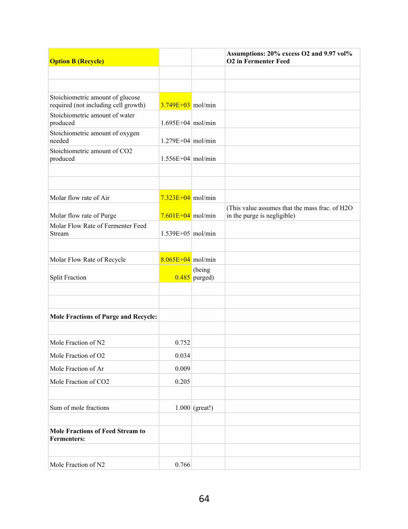
64
Option B (Recycle) Assumptions: 20% excess O2 and 9.97 vol% O2 in Fermenter Feed
Stoichiometric amount of glucose required (not including cell growth) 3.749E+03 mol/min
Stoichiometric amount of water produced 1.695E+04 mol/min
Stoichiometric amount of oxygen needed 1.279E+04 mol/min
Stoichiometric amount of CO2 produced 1.556E+04 mol/min
Molar flow rate of Air 7.323E+04 mol/min
Molar flow rate of Purge 7.601E+04 mol/min (This value assumes that the mass frac. of H2O in the purge is negligible)
Molar Flow Rate of Fermenter Feed Stream 1.539E+05 mol/min
Molar Flow Rate of Recycle 8.065E+04 mol/min
Split Fraction 0.485(being purged)
Mole Fractions of Purge and Recycle:
Mole Fraction of N2 0.752
Mole Fraction of O2 0.034
Mole Fraction of Ar 0.009
Mole Fraction of CO2 0.205
Sum of mole fractions 1.000 (great!)
Mole Fractions of Feed Stream to Fermenters:
Mole Fraction of N2 0.766

65
Mole Fraction of O2 0.1173
Mole Fraction of Ar 0.009
Mole Fraction of CO2 0.108
Sum of mole fractions 1.000 (great!)
Feed Stream to Absorber:
Molar Flow Rate 1.603E+05 mol/min (This assumes the exit stream leaving the fermenter is saturated with H2O)
Composition of Feed to Absorber:
Mole Fraction of N2 0.735
Mole Fraction of O2 0.016
Mole Fraction of isoprene 0.009
Mole Fraction of Ar 0.009
Mole Fraction of CO2 0.200
Mole Fraction of H2O 0.031
Sum of mole fractions 1.000 (great!)
Liquid Water leaving through the fermenter 1.198E+04 mol/min
Flow rate of isoprene-lean gas stream 1.539E+05 mol/min (This assumes a perfect separation between isoprene and the other gas-phase components)
(i.e. the gas stream leaving the top of the tower)
Composition of isoprene-lean gas stream:
Mole Fraction of N2 0.766
Mole Fraction of O2 0.017
Mole Fraction of Ar 0.009
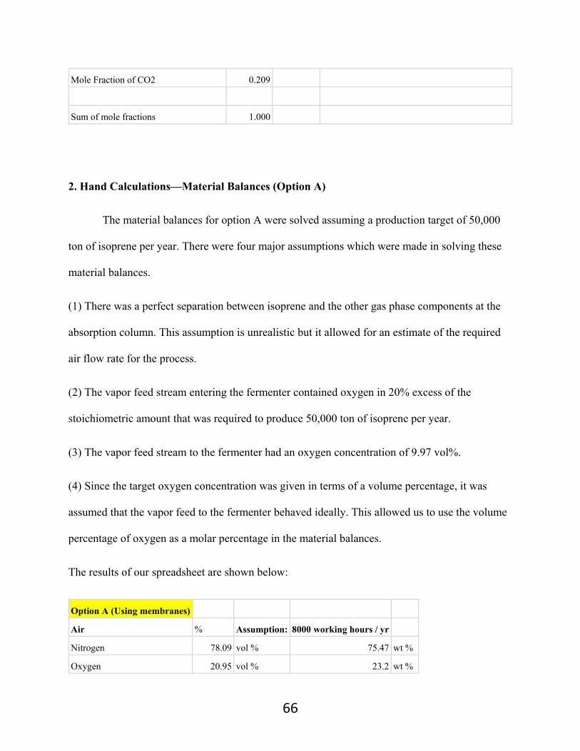
66
Mole Fraction of CO2 0.209
Sum of mole fractions 1.000
2. Hand Calculations—Material Balances (Option A)
The material balances for option A were solved assuming a production target of 50,000
ton of isoprene per year. There were four major assumptions which were made in solving these
material balances.
(1) There was a perfect separation between isoprene and the other gas phase components at the
absorption column. This assumption is unrealistic but it allowed for an estimate of the required
air flow rate for the process.
(2) The vapor feed stream entering the fermenter contained oxygen in 20% excess of the
stoichiometric amount that was required to produce 50,000 ton of isoprene per year.
(3) The vapor feed stream to the fermenter had an oxygen concentration of 9.97 vol%.
(4) Since the target oxygen concentration was given in terms of a volume percentage, it was
assumed that the vapor feed to the fermenter behaved ideally. This allowed us to use the volume
percentage of oxygen as a molar percentage in the material balances.
The results of our spreadsheet are shown below:
Option A (Using membranes)
Air % Assumption: 8000 working hours / yr
Nitrogen 78.09 vol % 75.47 wt %
Oxygen 20.95 vol % 23.2 wt %

67
Argon 0.933 vol % 1.28 wt %
Carbon Dioxide 0.027 vol % 0.05 wt %
Necessary O2 1.38E+11 L/yr 2.86E+05 L/min
Necessary Air 6.56E+11 L/yr 1.37E+06 L/min
Necessary N2 diluent 7.23E+11 L/yr 1.51E+06 L/min
Total Gas Inflow 1.38E+12 L/yr 2.87E+06 L/min
N2 moles 3.23E+10 moles
N2 mass 9.04E+08 kg
Liquid N2 vol 1.12E+06 m^3
2.95E+08 gal/yr
Liquid N2 vol 8.86E+05 gal/day
CO2 Volume 1.67E+11 L/yr
H2O moles 8.14E+09 moles/yr
H2O vol, liquid 4.52E+02 m^3/yr
3. Hand Calculations—Absorption Column
The number of actual stages for the column was estimated using the Kremser equation.
The calculations of the absorption factor, minimum flow rate of solvent required, and number of
stages are shown on the next page.

68
Kremser Calculations (Absorption)
Entering vapor flow rate to absorption column (V) 9.618E+03 kmol/hr
I'll use Raoult's Law to calculate the K-value of isoprene:
K-value of isoprene 0.591
(1 - phi) 0.9999
Lmin (minimum amount of absorbent rate) 5.682E+03 kmol/hr
I'll choose an operating absorbent flow rate of 1.5*Lmin
L 8.523E+03 kmol/hr
Absorption factor (A) 1.50 (Eq. 19.2)
Number of stages 20 stages
The diameter and height of the column were estimated using a flooding velocity
calculation outlined in Product and Process Design Principles by Seider, Seader, Lewin, and
Widagdo. The flow rates and densities for liquid and vapor products of the column were obtained
from our Aspen simulation. The estimates for the capacitance parameter, surface tension factor,
foaming factor, and hole-area factor were computed using the aforementioned methods.
The following assumptions were made for the flooding velocity calculations:
(1) A tray column will be used with 24 in. spacing between trays.
(2) The trays are non-foaming.
(3) Sieve trays will be used.
The results of our Excel spreadsheet are shown on the next page.

69
Flooding Velocity Calculations (Absorber):
Mass flow rate of liquid leaving the bottom of the column (L*) 1.748E+06 lb/hr
Density of liquid stream (ρ_L) 45.323 lb/ft^3
Mass flow rate of gas leaving the top of the column (G*) 6.352E+05 lb/hr
Density of gas stream (ρ_G) 0.131 lb/ft^3
Flow ratio parameter (F_LG) 0.148
C_SB 0.107 m/s
Surface Tension of liquid stream leaving bottom of absorber 25.6 dyne/cm
F_ST (Surface Tension Factor) 1.05
F_f (Foaming Factor) 1
F_HA (Hole‐area Factor) 1
C (Capacity parameter) 0.112
U_f (Flooding Velocity) 2.458E+04 ft/hr
Ratio of downcomer area to tower's internal cross‐sectional area (A_d/A_T) 0.105
I'm going to compute the diameter of the column using 0.85*U_f
D (Diameter of column) 18.2 ft
Tower Height 54.0 ft
Note: The diameter and height that were obtained using our hand calculations were not used in
our profitability analysis. Aspen’s estimates were used instead.
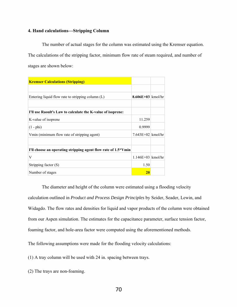
70
4. Hand calculations—Stripping Column
The number of actual stages for the column was estimated using the Kremser equation.
The calculations of the stripping factor, minimum flow rate of steam required, and number of
stages are shown below:
Kremser Calculations (Stripping)
Entering liquid flow rate to stripping column (L) 8.606E+03 kmol/hr
I'll use Raoult's Law to calculate the K-value of isoprene:
K-value of isoprene 11.259
(1 - phi) 0.9999
Vmin (minimum flow rate of stripping agent) 7.643E+02 kmol/hr
I'll choose an operating stripping agent flow rate of 1.5*Vmin
V 1.146E+03 kmol/hr
Stripping factor (S) 1.50
Number of stages 20
The diameter and height of the column were estimated using a flooding velocity
calculation outlined in Product and Process Design Principles by Seider, Seader, Lewin, and
Widagdo. The flow rates and densities for liquid and vapor products of the column were obtained
from our Aspen simulation. The estimates for the capacitance parameter, surface tension factor,
foaming factor, and hole-area factor were computed using the aforementioned methods.
The following assumptions were made for the flooding velocity calculations:
(1) A tray column will be used with 24 in. spacing between trays.
(2) The trays are non-foaming.

71
(3) Sieve trays will be used.
The results of our Excel spreadsheet are shown below.
Flooding Velocity Calculations (Stripping)
Mass flow rate of liquid leaving the bottom of the column (L*) 3.043E+06 lb/hr
Density of liquid stream (ρ_L) 43.412 lb/ft^3
Mass flow rate of gas leaving the top of the column (G*) 6.968E+05 lb/hr
Density of gas stream (ρ_G) 0.079 lb/ft^3
Flow ratio parameter (F_LG) 0.187
C_SB 0.099 m/s
Surface Tension of liquid stream leaving bottom of absorber 17.8 dyne/cm
F_ST (Surface Tension Factor) 0.98
F_f (Foaming Factor) 1
F_HA (Hole-area Factor) 1
C (Capacity parameter) 0.097
U_f (Flooding Velocity) 2.673E+04 ft/hr
Ratio of downcomer area to tower's internal cross-sectional area (A_d/A_T) 0.110
I'm going to compute the diameter of the column using 0.85*U_f
D (Diameter of column) 23.5 ft
Tower Height 54.0 ft
Note: The diameter and height that were obtained using our hand calculations were not used in
our profitability analysis. Aspen’s estimates were used instead.

72
5. Hand Calculations—Shell and Tube Heat Exchanger (Fermenters)
The calculations of the sizes and flow rates for the fermenter’s shell and tube heat
exchangers were described in the Equipment List and Unit Descriptions section. The results of
our excel spreadsheet are shown below.
Heat Exchangers for Fermenters
Total Q -4.512E+08 kJ/hr
Q per fermenter -1.504E+08 kJ/hr
Using Aspen, I obtained the heat capacity for the liquid that's leaving the fermenter
Cp 0.0745814736 kJ/mol-K
Upper limit on the fermenter's temperature 34 °C
Target Temperature 25 °C
Molar flow rate of hot stream to the heat exchanger 2.241E+08 mol/hr
We're using cooling water at 5°C and 1 atm
Initial temperature of cooling water 5 °C
Final temperature of cooling water 15 °C
Mass flow rate of cooling water 3.598E+06 kg/hr
Note: We'll need five identical heat exchangers (only three will be operated at any given time)
Total cooling water requirement for fermenters 1.079E+07 kg/hr
Sizing Calculations for Heat Exchangers (for fermenters):
Log-mean temperature difference 35.09 °F

73
Next, I estimated the overall heat transfer coefficient using Table 18.5 in the Product and Process Design text)
Note: This assumes that the cooling water is on the *shell* side and the liquid that's leaving the fermenter is on the *tube* side
U 225 BTU/°F-ft^2-hr
Next, I need to estimate the correction factor F_T
R 0.900
S 0.345
F_T (Correction Factor) 0.959
Ai (Heat Transfer Area) 18805.64 ft^2
I'm going to select a stream velocity of 17 ft/s for the tube side:
u 17 ft/s
Total cross-sectional area per pass 2.077 ft^2
Assuming that we have tubes with the following sizes:
O.D 0.75 in
I.D 0.62 in
Number of tubes per pass 991 tubes
I'm going to select a tube length of 16 ft
L 16 ft
Heat transfer area per tube 2.597 ft^2
Number of tube passes 7 passes
Assuming the tubes are on a 1-in square pitch
Total number of tubes 7241 tubes
Inner Diameter of Shell (D_s) 170.32 in
Baffle spacing:
b_min 34.06498257 in

74
b_max 170.32 in
I'm going to select a baffle spacing that's directly in the midle of this range
b 102.19 in
6. Hand Calculations—Shell and Tube Heat Exchanger (Air Stream)
The calculations of the sizes and flow rates for the air stream’s shell and tube heat
exchanger were described in the Equipment List and Unit Descriptions section. The results of
our excel spreadsheet are shown below.
Sizing Calculations (for the air stream's HX)
Mass flow rate of air stream 1.273E+05 kg/hr
Initial temp of air 90.84755 °C
Final temp of air 34 °C
Heat capacity of air 1.0005 kJ/kg-K
Q 7.238E+06 kJ/hr
Initial temp of cooling water 25 °C
Final temp of cooling water 80 °C
Mass flow rate of cooling water 3.148E+04 kg/hr
Log-mean temperature difference 17.811 °F
Next, I estimated the overall heat transfer coefficient using Table 18.5 in the Product and Process Design text)
Note: This assumes that the cooling water is on the *tube* side and air is on the *shell* side
U 60 BTU/°F-ft^2-hr

75
Next, I need to estimate the correction factor F_T
R 1.034
S 0.835
F_T (Correction Factor) 1.000 (I'll fix this later)
Ai (Heat Transfer Area) 6,414.10 ft^2
I'm going to select a stream velocity of 0.4 ft/s for the tube side:
u 0.3 ft/s
Total cross-sectional area per pass 1.030 ft^2
Assuming that we have tubes with the following sizes:
O.D 0.75 in
I.D 0.62 in
Number of tubes per pass 491 tubes
I'm going to select a tube length of 16 ft
L 16 ft
Heat transfer area per tube 2.597 ft^2
Number of tube passes 5 passes
Assuming the tubes are on a 1-in square pitch
Total number of tubes 2470 tubes
Inner Diameter of Shell (D_s) 70.23 in
Baffle spacing:
b_min 14.04517081 in
b_max 70.23 in
I'm going to select a baffle spacing that's directly in the midle of this range
b 42.14 in

76
7. Hand Calculations—Shell and Tube Heat Exchanger (Flash Vessel)
The calculations of the sizes and flow rates for the heat exchanger for the flash vessel’s
feed were described in the Equipment List and Unit Descriptions section. The results of our excel
spreadsheet are shown below.
Sizing Calculations (HX for the Flash Vessel's Feed)
Required Heat Duty 20748180.72 kJ/hr
Inlet temp. of vapor stream 98.9 °C
Outet temp. of vapor stream 15 °C
Initial temp. of chilled water 5 °C
Final temp. of chilled water 85 °C
Note: We're using chilled water at 5 degrees C and 1 atm
Mass flow rate of chilled water 61986.68 kg/hr
Log-mean temperature difference 21.309 °F
Next, I estimated the overall heat transfer coefficient using Table 18.5 in the Product and Process Design text)
Note: This assumes that the cooling water is on the *tube* side and the vapor is on the *shell* side
U 60 BTU/°F-ft^2-hr
Next, I need to estimate the correction factor F_T
R 1.05
S 0.852
F_T (Correction Factor) 1.000
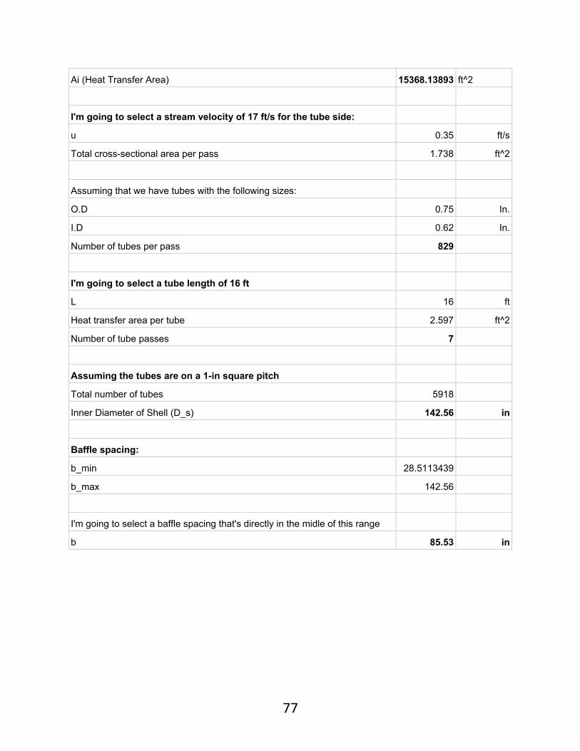
77
Ai (Heat Transfer Area) 15368.13893 ft^2
I'm going to select a stream velocity of 17 ft/s for the tube side:
u 0.35 ft/s
Total cross-sectional area per pass 1.738 ft^2
Assuming that we have tubes with the following sizes:
O.D 0.75 In.
I.D 0.62 In.
Number of tubes per pass 829
I'm going to select a tube length of 16 ft
L 16 ft
Heat transfer area per tube 2.597 ft^2
Number of tube passes 7
Assuming the tubes are on a 1-in square pitch
Total number of tubes 5918
Inner Diameter of Shell (D_s) 142.56 in
Baffle spacing:
b_min 28.5113439
b_max 142.56
I'm going to select a baffle spacing that's directly in the midle of this range
b 85.53 in

78
8. Hand Calculations—Flash Vessel
As was mentioned in the Equipment Lists and Unit Descriptions section, the diameter and
height of the flash vessel were computed using the methods outlined in Separation Process
Engineering: Includes Mass Transfer Analysis (3rd edition) by Phillip C. Wankat. A flooding
velocity calculation was used and 85% of the flooding velocity was chosen. The detailed
calculations are shown below:
Flash Vessel Sizing
Liquid flow rate 30458.57 lb/hr
Vapor flow rate 5503.329 lb/hr
Density of liquid phase 53.66 lb/ft^3
Density of vapor phase 0.21 lb/ft^3
F_lv 0.348
K_drum 0.298 ft/s
U_perm 4.72 ft/s
We're going to use 85% of the flooding velocity for our calculations
U 4.016024592 ft/s
Cross-sectional area (A_c) 1.79056846 ft^2
Diameter of flash vessel 1.51 ft
Assuming a height-to-diameter ratio of 5
Height of flash vessel 7.55 ft

79
9. Aspen Flow Sheet
The Aspen flow sheet is essentially the same as the process flow diagram. The only
notable difference is that the fermenters were modeled using the RSTOIC and flash vessel
modules in Aspen. Since it isn’t possible to specify two separate phases as effluent streams for
RSTOIC, a flash vessel had to be used to separate the liquid and vapor phases for the fermenter.
Even though the fermenter was modeled as a continuous process, it is in fact a batch
process. Our scheduling of the fermenters allowed for the continuous production of isoprene in
the vapor phase but the liquid phase; however, was removed at the end of every 72 hour batch.
Even though a continuous process was simulated, the results of the simulations were used to
estimate the compositions of the vapor and liquid phases of the fermenter, which were valid even
though the removal of the liquid contents of the fermenters was inherently a batch process.
Therefore, it allowed us to estimate the amount of isoprene that was lost after every fermentation
batch since the flow rate of the liquid phase was easily converted to a batch value. The amount of
liquid that accumulated in the fermenter was simply 72 hours times the liquid flow rate that was
obtained from Aspen.
The other unit operations are the same as the ones that were listed in the process flow
sheet, and no further explanations are necessary.