large-scale drivers of australian east coast cyclones since 1851 · corresponding author: stuart...

Browning. Journal of Southern Hemisphere Earth Systems Science (2016) 66: 125–151

Corresponding author: Stuart Browning, Department of Environmental Sciences, Macquarie University, Sydney NSW 2109, Australia. Email: [email protected]

Large-scale drivers of Australian East Coast Cyclones since 1851

Stuart A. Browning and Ian D. Goodwin

Marine Climate Risk Group, Department of Environmental Sciences, Macquarie University, Sydney, Australia

(Manuscript received September 2015; accepted May 2016)

Subtropical maritime low-pressure systems are one of the most complex and destructive storm types to impact Australia’s eastern seaboard. This family of storms, commonly referred to as East Coast Cyclones (ECC), is most active during the late autumn and early winter period when baroclinicity increases in the Tasman Sea region. ECC have proven challenging to forecast at both event and seasonal timescales. Storm activity datasets, objectively determined from reanalyses using cyclone detection algorithms, have improved understanding of the drivers of ECC over the era of satellite data coverage. In this study we attempt to extend these datasets back to 1851 using the Twentieth Century Reanalysis version 2c (20CRv2c). However, uncertainty in the 20CRv2c increases back through time due to observational data scarcity, and individual cyclones counts tend to be underestimated during the 19th century. An alternative approach is explored whereby storm activity is estimated from seasonal atmosphere-ocean circulation patterns. Seasonal ECC frequency over the 1955 to 2014 period is significantly correlated to regional sea-level pressure and sea surface temperature (SST) patterns. These patterns are used to downscale the 20CRv2c during early years when individual events are not well simulated. The stormiest periods since 1851 appear to have been 1870 to the early 1890s, and 1950 to the early 1970s. Total storm activity has been below the long-term average for most winters since 1976. Conditions conducive to frequent ECC events tend to occur during periods of relatively warm SST in the southwest Pacific typical of negative Interdecadal Pacific Oscillation (IPO-ve). Extratropical cyclogenesis is associated with negative Southern Annular Mode (SAM-ve) and blocking in the southern Tasman Sea. Subtropical cyclogenesis is associated with SAM+ve and blocking in the central Tasman Sea. While the downscaling approach shows some skill at estimating seasonal storm activity from the large-scale circulation, it cannot overcome data scarcity based uncertainties in the 19th century when the 20CRv2c is effectively unconstrained throughout most of the southern hemisphere. Storm frequency estimates during the 19th century are difficult to verify and should be interpreted cautiously and with reference to available documentary evidence.

1. Introduction

Australia’s eastern seaboard is periodically impacted by severe subtropical maritime storms. Commonly known as East Coast Lows (ECL) or East Coast Cyclones (ECC), these storms have proven most frequent during late autumn and early winter yet can occur at any time of year. Because ECCs tend to impact the more populated latitudes of Australia’s eastern seaboard, insured losses from extreme ECC can exceed those of severe tropical cyclone events (ICA, 2015). ECC predictability remains poor at both event (Mills et al. 2010) and seasonal timescales. Recent studies have provided insights into ECC frequency and large-scale drivers since ~1980 using objective cyclone detection algorithms applied to reanalysis data (Browning and Goodwin 2013, Pepler et al. 2015). However, extreme ECC events are relatively infrequent, having an apparent decadal to multidecadal return period, meaning that the past ~30–40 years are probably insufficient

Browning. Large-scale drivers of East Coast Cyclones

126

to capture the full range of ECC variability. The 1950s to 1970s are believed to have been the stormiest decades of the 20th century and some of the most extreme documented events occurred during the late 19th century (Callaghan and Helman 2008)—a longer record is therefore desirable.

The skill of cyclone detection algorithms is largely dependent on data quality (Allen et al. 2010). Pepler and Coutts-Smith (2013) recently developed a 58-year (1950–2008) Tasman Sea storm history by applying the Melbourne University Tracking Scheme (Murray and Simmonds 1991, Jones and Simmonds 1993) to the NCEP1 reanalysis (Kalnay et al. 1996). Unfortunately, NCEP1 contains several well-documented data errors in the southern hemisphere (Bromwich and Fogt 2004, Hines et al. 2000) that may affect results. The 20th Century Reanalysis Version 2c (20CRv2c) covers an even longer (1851–2014) period and is free from many of the errors affecting NCEP-1 (Compo et al. 2010). The 20CR has previously been used to develop retrospective analysis of both tropical and extratropical cyclone frequency (Wang et al. 2013).

The longer cyclone record afforded by the 20CRv2c should provide insights into decadal variability in ECC frequency and associated regional climate drivers. The 20CRv2c is constrained by surface pressure observations, of which there is sufficient spatial density in the Australia–New Zealand region post ~1955, however prior to this there is a progressive decrease in the density of observational data back through time. This means that any attempt to understand ECC variability from the 20CRv2c must contend with increasing data uncertainty back in time. Wang et al. (2012) found that as data density decreased, so too did the ability of the 20CRv2c ensemble mean to accurately simulate individual cyclones; therefore, in order to obtain more realistic results cyclone detection should be applied to the individual ensemble members.

An alternative approach to dealing with data uncertainty is to estimate cyclone activity at seasonal timescales using information about the large-scale seasonal drivers of ECC storm activity, as described in Browning and Goodwin (2013). Statistical downscaling uses the relationships between observations and large-scale features to estimate the behaviour of smaller scale feature such as cyclones that might not be accurately simulated (Caron et al. 2011, Pielke and Wilby 2012). Downscaling has been successfully used to estimate storm behaviour from both global climate model (GCM) data (Hunt and Watterson 2010, Daloz et al. 2012) and reanalysis data (Emanuel 2010, Elison Timm et al. 2013). An important caveat to downscaling—whether applied to GCM output or the 20CRv2c—is that the large-scale features of ocean and atmosphere circulation must be realistically simulated.

The primary aim of this paper is to develop a long (1851–2014) objectively determined history of ECC activity. To this effect we explore two complementary approaches: (i) extend the presently available ERA-Interim based storm day history (Browning and Goodwin 2013) by applying the same cyclone detection-tracking-classification algorithm to the longer 20CRv2c, and (ii) use statistical relationships between the storm day history and large-scale coupled ocean-atmosphere variability to develop a seasonal index representing storm activity. The paper is outlined as follows: Section 2 describe the application of cyclone detection, tracking and classification to the 20CRv2c sea-level pressure (SLP) data, and the development of a downscaling approach to estimate storm activity during the early decades of the 20CRv2c when individual events might not be well simulated. Section 3 presents the multidecadal history of storm conditions and investigates dynamical linkages between individual event frequency and large-scale patterns of seasonal climate variability. Section 4 focuses on the relationship between ECC activity and Pacific decadal variability, and evaluates some of the advantages and limitations of the downscaling approach. Section 5 provides some closing remarks, focusing primarily on the approach and its potential application to other climate datasets.

2. Data and methods

2.1 Data

This study uses the Twentieth Century Reanalysis project, as described in Compo et al. (2011), as its primary source of atmospheric data. 20CRv2c (the current research version) has a spatial resolution of 2° latitude/longitude and was developed using a Kalman Ensemble filter data assimilation; the model used is an experimental version of the NCEP_GFS that accounts for both volcanic and CO2 forcing. Gridded fields are constructed from a 56-member ensemble mean. 20CRv2c uses sea-level pressure (SLP) observations from the International Surface Pressure Databank (ISPD) version 3.2.9, sea surface temperature (SST) from Simple Ocean Data Assimilation with sparse input (SODAsi.2), and sea ice boundary conditions from the COBE-SST2 (Hirahara et al. 2014). 20CRv2c data are provided by the National Ocean Atmosphere


127

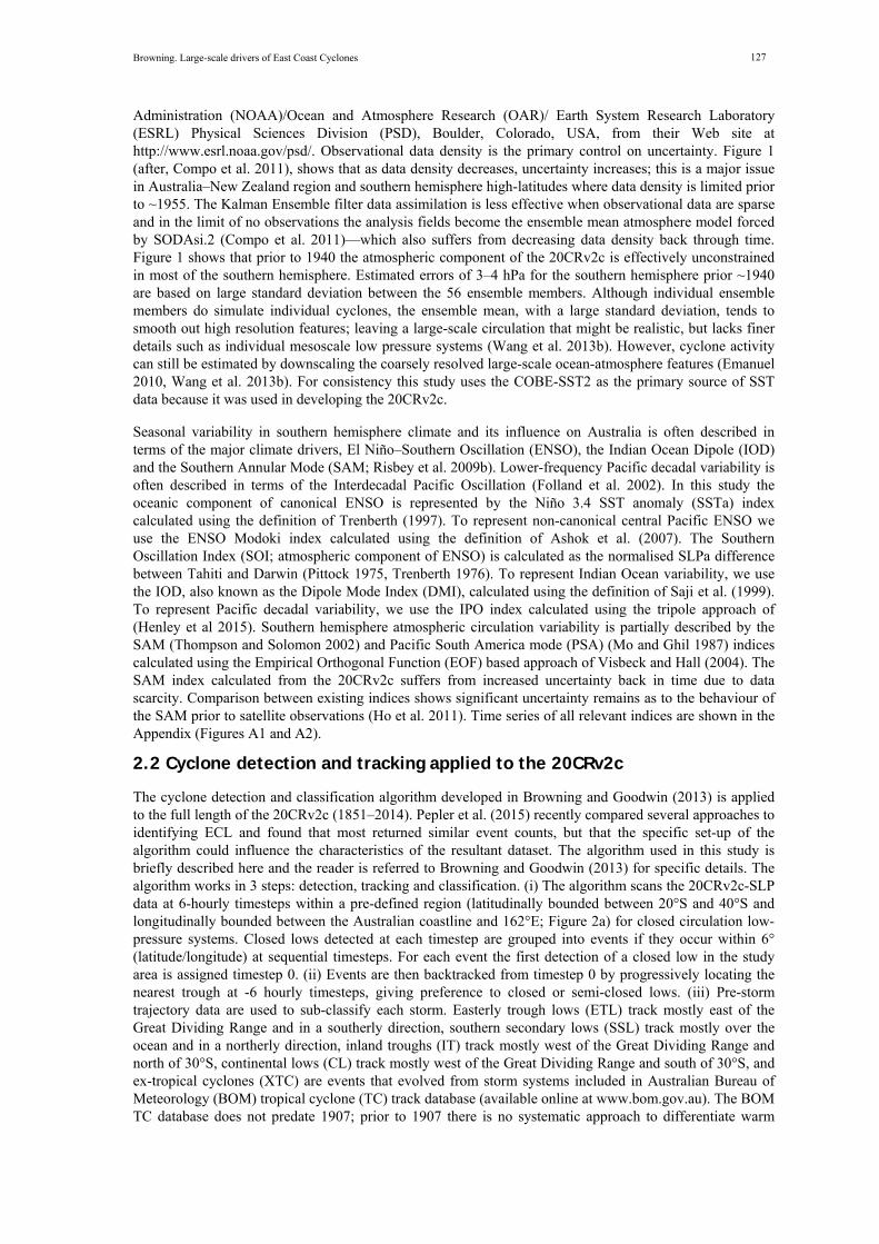
Administration (NOAA)/Ocean and Atmosphere Research (OAR)/ Earth System Research Laboratory (ESRL) Physical Sciences Division (PSD), Boulder, Colorado, USA, from their Web site at http://www.esrl.noaa.gov/psd/. Observational data density is the primary control on uncertainty. Figure 1 (after, Compo et al. 2011), shows that as data density decreases, uncertainty increases; this is a major issue in Australia–New Zealand region and southern hemisphere high-latitudes where data density is limited prior to ~1955. The Kalman Ensemble filter data assimilation is less effective when observational data are sparse and in the limit of no observations the analysis fields become the ensemble mean atmosphere model forced by SODAsi.2 (Compo et al. 2011)—which also suffers from decreasing data density back through time. Figure 1 shows that prior to 1940 the atmospheric component of the 20CRv2c is effectively unconstrained in most of the southern hemisphere. Estimated errors of 3–4 hPa for the southern hemisphere prior ~1940 are based on large standard deviation between the 56 ensemble members. Although individual ensemble members do simulate individual cyclones, the ensemble mean, with a large standard deviation, tends to smooth out high resolution features; leaving a large-scale circulation that might be realistic, but lacks finer details such as individual mesoscale low pressure systems (Wang et al. 2013b). However, cyclone activity can still be estimated by downscaling the coarsely resolved large-scale ocean-atmosphere features (Emanuel 2010, Wang et al. 2013b). For consistency this study uses the COBE-SST2 as the primary source of SST data because it was used in developing the 20CRv2c.

Seasonal variability in southern hemisphere climate and its influence on Australia is often described in terms of the major climate drivers, El Niño–Southern Oscillation (ENSO), the Indian Ocean Dipole (IOD) and the Southern Annular Mode (SAM; Risbey et al. 2009b). Lower-frequency Pacific decadal variability is often described in terms of the Interdecadal Pacific Oscillation (Folland et al. 2002). In this study the oceanic component of canonical ENSO is represented by the Niño 3.4 SST anomaly (SSTa) index calculated using the definition of Trenberth (1997). To represent non-canonical central Pacific ENSO we use the ENSO Modoki index calculated using the definition of Ashok et al. (2007). The Southern Oscillation Index (SOI; atmospheric component of ENSO) is calculated as the normalised SLPa difference between Tahiti and Darwin (Pittock 1975, Trenberth 1976). To represent Indian Ocean variability, we use the IOD, also known as the Dipole Mode Index (DMI), calculated using the definition of Saji et al. (1999). To represent Pacific decadal variability, we use the IPO index calculated using the tripole approach of (Henley et al 2015). Southern hemisphere atmospheric circulation variability is partially described by the SAM (Thompson and Solomon 2002) and Pacific South America mode (PSA) (Mo and Ghil 1987) indices calculated using the Empirical Orthogonal Function (EOF) based approach of Visbeck and Hall (2004). The SAM index calculated from the 20CRv2c suffers from increased uncertainty back in time due to data scarcity. Comparison between existing indices shows significant uncertainty remains as to the behaviour of the SAM prior to satellite observations (Ho et al. 2011). Time series of all relevant indices are shown in the Appendix (Figures A1 and A2).

2.2 Cyclone detection and tracking applied to the 20CRv2c

The cyclone detection and classification algorithm developed in Browning and Goodwin (2013) is applied to the full length of the 20CRv2c (1851–2014). Pepler et al. (2015) recently compared several approaches to identifying ECL and found that most returned similar event counts, but that the specific set-up of the algorithm could influence the characteristics of the resultant dataset. The algorithm used in this study is briefly described here and the reader is referred to Browning and Goodwin (2013) for specific details. The algorithm works in 3 steps: detection, tracking and classification. (i) The algorithm scans the 20CRv2c-SLP data at 6-hourly timesteps within a pre-defined region (latitudinally bounded between 20°S and 40°S and longitudinally bounded between the Australian coastline and 162°E; Figure 2a) for closed circulation low-pressure systems. Closed lows detected at each timestep are grouped into events if they occur within 6° (latitude/longitude) at sequential timesteps. For each event the first detection of a closed low in the study area is assigned timestep 0. (ii) Events are then backtracked from timestep 0 by progressively locating the nearest trough at -6 hourly timesteps, giving preference to closed or semi-closed lows. (iii) Pre-storm trajectory data are used to sub-classify each storm. Easterly trough lows (ETL) track mostly east of the Great Dividing Range and in a southerly direction, southern secondary lows (SSL) track mostly over the ocean and in a northerly direction, inland troughs (IT) track mostly west of the Great Dividing Range and north of 30°S, continental lows (CL) track mostly west of the Great Dividing Range and south of 30°S, and ex-tropical cyclones (XTC) are events that evolved from storm systems included in Australian Bureau of Meteorology (BOM) tropical cyclone (TC) track database (available online at www.bom.gov.au). The BOM TC database does not predate 1907; prior to 1907 there is no systematic approach to differentiate warm


128

season ETLs from transitioning TCs. This is not a major problem for this work, as we are focused primarily on the cool season when ECC are most frequent and TCs are uncommon. Thresholds for storm intensity and duration were applied to exclude minor systems: only storms lasting for longer than 18 hours and developing a pressure gradient of at least 6 hPa per 2° latitude/longitude were retained.

Figure 1 Data density in the The International Surface Pressure Databank version 3 as used in the 20CRv2c (Compo et al. 2015). (a) Spatial distribution of station data included in each year of the 20CRv2c. (b) Temporal change in data density in the Australian (red), New Zealand (green) and Antarctic (blue) regions (regions used to calculate station data density are illustrated in (a)); dashed line at 1955 denotes reduction in data density. (c) Compo et al. (2011) figure 6.3b showing the relationship between data density and error in the southern hemisphere—note the logarithmic scale.

2.3 Comparison between cyclone tracking applied to ERA-Interim and 20CRv2c

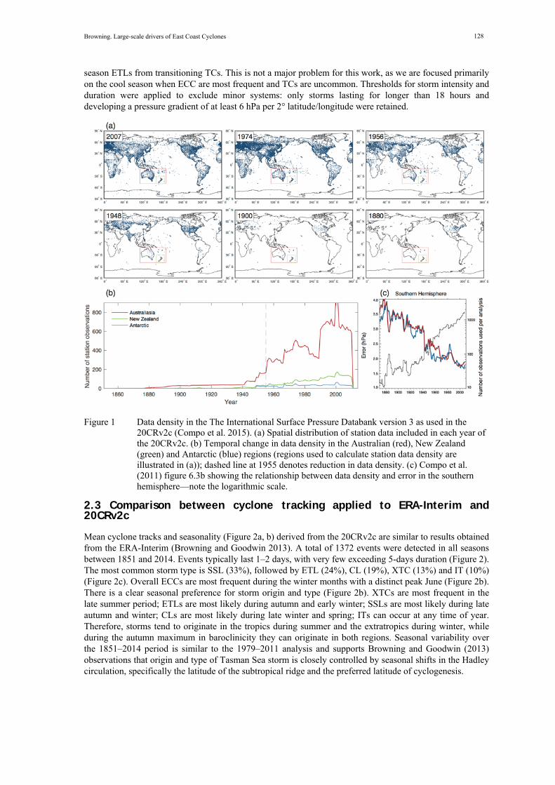
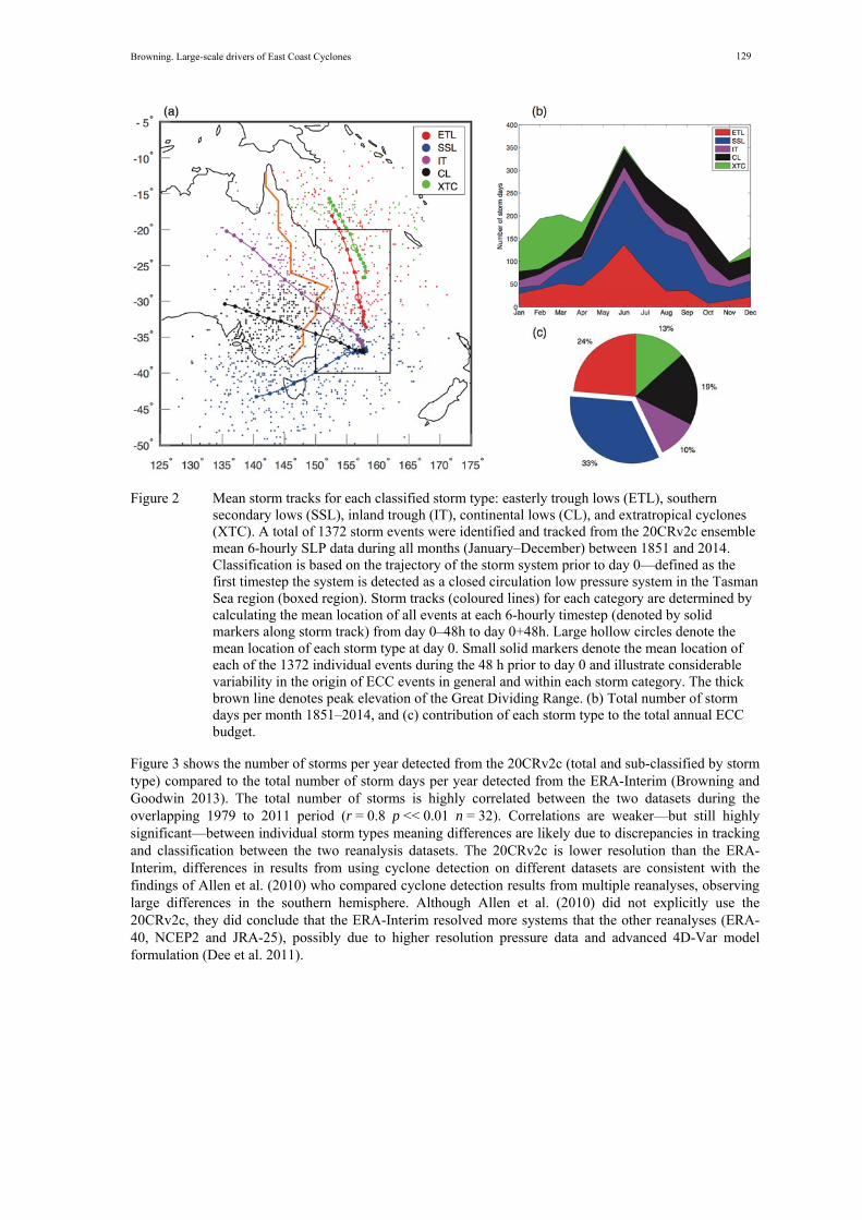
Mean cyclone tracks and seasonality (Figure 2a, b) derived from the 20CRv2c are similar to results obtained from the ERA-Interim (Browning and Goodwin 2013). A total of 1372 events were detected in all seasons between 1851 and 2014. Events typically last 1–2 days, with very few exceeding 5-days duration (Figure 2). The most common storm type is SSL (33%), followed by ETL (24%), CL (19%), XTC (13%) and IT (10%) (Figure 2c). Overall ECCs are most frequent during the winter months with a distinct peak June (Figure 2b). There is a clear seasonal preference for storm origin and type (Figure 2b). XTCs are most frequent in the late summer period; ETLs are most likely during autumn and early winter; SSLs are most likely during late autumn and winter; CLs are most likely during late winter and spring; ITs can occur at any time of year. Therefore, storms tend to originate in the tropics during summer and the extratropics during winter, while during the autumn maximum in baroclinicity they can originate in both regions. Seasonal variability over the 1851–2014 period is similar to the 1979–2011 analysis and supports Browning and Goodwin (2013) observations that origin and type of Tasman Sea storm is closely controlled by seasonal shifts in the Hadley circulation, specifically the latitude of the subtropical ridge and the preferred latitude of cyclogenesis.


129

Figure 2 Mean storm tracks for each classified storm type: easterly trough lows (ETL), southern secondary lows (SSL), inland trough (IT), continental lows (CL), and extratropical cyclones (XTC). A total of 1372 storm events were identified and tracked from the 20CRv2c ensemble mean 6-hourly SLP data during all months (January–December) between 1851 and 2014. Classification is based on the trajectory of the storm system prior to day 0—defined as the first timestep the system is detected as a closed circulation low pressure system in the Tasman Sea region (boxed region). Storm tracks (coloured lines) for each category are determined by calculating the mean location of all events at each 6-hourly timestep (denoted by solid markers along storm track) from day 0–48h to day 0+48h. Large hollow circles denote the mean location of each storm type at day 0. Small solid markers denote the mean location of each of the 1372 individual events during the 48 h prior to day 0 and illustrate considerable variability in the origin of ECC events in general and within each storm category. The thick brown line denotes peak elevation of the Great Dividing Range. (b) Total number of storm days per month 1851–2014, and (c) contribution of each storm type to the total annual ECC budget.

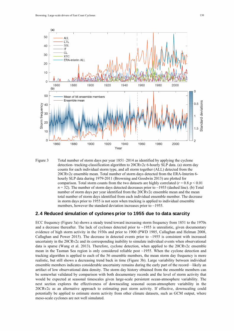
Figure 3 shows the number of storms per year detected from the 20CRv2c (total and sub-classified by storm type) compared to the total number of storm days per year detected from the ERA-Interim (Browning and Goodwin 2013). The total number of storms is highly correlated between the two datasets during the overlapping 1979 to 2011 period (r = 0.8 p << 0.01 n = 32). Correlations are weaker—but still highly significant—between individual storm types meaning differences are likely due to discrepancies in tracking and classification between the two reanalysis datasets. The 20CRv2c is lower resolution than the ERA-Interim, differences in results from using cyclone detection on different datasets are consistent with the findings of Allen et al. (2010) who compared cyclone detection results from multiple reanalyses, observing large differences in the southern hemisphere. Although Allen et al. (2010) did not explicitly use the 20CRv2c, they did conclude that the ERA-Interim resolved more systems that the other reanalyses (ERA-40, NCEP2 and JRA-25), possibly due to higher resolution pressure data and advanced 4D-Var model formulation (Dee et al. 2011).


130

Figure 3 Total number of storm days per year 1851–2014 as identified by applying the cyclone detection- tracking-classification algorithm to 20CRv2c 6-hourly SLP data. (a) storm day counts for each individual storm type, and all storm together (ALL) detected from the 20CRv2c ensemble mean. Total number of storm days detected from the ERA-Interim 6-hourly SLP data during 1979-2011 (Browning and Goodwin 2013) are plotted for comparison. Total storm counts from the two datasets are highly correlated (r = 0.8 p < 0.01 n = 32). The number of storm days detected decreases prior to ~1955 (dashed line). (b) Total number of storm days per year identified from the 20CRv2c ensemble mean and the mean total number of storm days identified from each individual ensemble member. The decrease in storm days prior to 1955 is not seen when tracking is applied to individual ensemble members, however the standard deviation increases prior to ~1955.

2.4 Reduced simulation of cyclones prior to 1955 due to data scarcity

ECC frequency (Figure 3a) shows a steady trend toward increasing storm frequency from 1851 to the 1970s and a decrease thereafter. The lack of cyclones detected prior to ~1955 is unrealistic, given documentary evidence of high storm activity in the 1930s and prior to 1900 (PWD 1985, Callaghan and Helman 2008, Callaghan and Power 2015). The decrease in detected events prior to ~1955 is consistent with increased uncertainty in the 20CRv2c and its corresponding inability to simulate individual events when observational data is sparse (Wang et al. 2013). Therefore, cyclone detection, when applied to the 20CRv2c ensemble mean in the Tasman Sea region is only considered reliable post ~1955. When the cyclone detection and tracking algorithm is applied to each of the 56 ensemble members, the mean storm day frequency is more realistic, but still shows a decreasing trend back in time (Figure 3b). Large variability between individual ensemble members indicates considerable uncertainty remains during the early part of the record—likely an artifact of low observational data density. The storm day history obtained from the ensemble members can be somewhat validated by comparison with both documentary records and the level of storm activity that would be expected at seasonal timescales given large-scale persistent ocean-atmosphere variability. The next section explores the effectiveness of downscaling seasonal ocean-atmosphere variability in the 20CRv2c as an alternative approach to estimating past storm activity. If effective, downscaling could potentially be applied to estimate storm activity from other climate datasets, such as GCM output, where meso-scale cyclones are not well simulated.


131

2.5 Downscaling the early portion of the 20CRv2c using large-scale driver relationships established over the 1955–2014 period

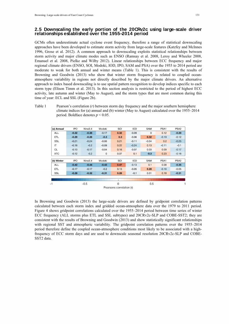
GCMs often underestimate actual cyclone event frequency, therefore a range of statistical downscaling approaches have been developed to estimate storm activity from large-scale features (Katzfey and McInnes 1996, Grose et al. 2012). A common approach to downscaling exploits statistical relationships between storm activity and major climate modes such as ENSO (Ramsay et al. 2008, Leroy and Wheeler 2008, Emanuel et al. 2008, Pielke and Wilby 2012). Linear relationships between ECC frequency and major regional climate drivers (ENSO, SOI, Modoki, IOD, IPO, SAM and PSA) over the 1955 to 2014 period are moderate to weak for both annual and winter means (Table 1). This is consistent with the results of Browning and Goodwin (2013) who show that winter storm frequency is related to coupled ocean-atmosphere variability in regions not directly described by the major climate drivers. An alternative approach to index based downscaling is to use spatial pattern recognition to develop indices specific to each storm type (Elison Timm et al. 2013). In this section analysis is restricted to the period of highest ECC activity, late autumn and winter (May to August), and the storm types that are most common during this time of year: ECL and SSL (Figure 2b).

Table 1 Pearson’s correlation (r) between storm day frequency and the major southern hemisphere climate indices for (a) annual and (b) winter (May to August) calculated over the 1955–2014 period. Boldface denotes p < 0.05.

In Browning and Goodwin (2013) the large-scale drivers are defined by gridpoint correlation patterns calculated between each storm index and gridded ocean-atmosphere data over the 1979 to 2011 period. Figure 4 shows gridpoint correlations calculated over the 1955–2014 period between time series of winter ECC frequency (ALL storms plus ETL and SSL subtypes) and 20CRv2c-SLP and COBE-SST2; they are consistent with the results of Browning and Goodwin (2013) and show statistically significant relationships with regional SST and atmospheric variability. The gridpoint correlation patterns over the 1955–2014 period therefore define the coupled ocean-atmosphere conditions most likely to be associated with a high-frequency of ECC storm days and are used to downscale seasonal resolution 20CRv2c-SLP and COBE-SST2 data.


132

Figure 4 Gridpoint Pearson’s correlation (r) between seasonal (May to August) ECC storm frequency and (1) COBE-SST2 and (2) 20CRv2c SLP calculated over 1955 to 2014: (a) ALL storms, (b) ETL, and (c) SSL. Stippling shows regions with p < 0.05. Red box denotes region used for spatial pattern downscaling—see text for more detail.

The downscaling approach is conceptually similar to the approach used by Elison Timm et al. (2013) and utilises spatial correlations to rank each season of the 20CRv2c-SLP and COBE-SST2 by its similarity to the respective gridpoint correlation fields shown in Figure 4. Seasonal spatial similarity indices are calculated from 20CRv2c-SLP and COBE-SST2 for each storm type. In all cases the spatial similarity indices are significantly (p < 0.01) correlated to the original storm day time series over the calibration period (1955–2014) and the full 1851–2014 time period (Figure 5, columns 1 and 2). The SST and SLP spatial similarity indices are averaged to produce a single index that, for ALL storms and ETL is better correlated to storm day frequency than its components (Figure 5, column 3). The original 1955–2014 storm day time series are also better correlated to the spatial similarity indices than to any of the major climate drivers shown in Table 1.

500 hPa geopotential height (GPH) data were also evaluated, but omitted from the final indices. Although upper atmospheric dynamics have been shown to be important in ECC development (Bridgman 1985, Dowdy et al. 2013, Mills et al. 2010), the final indices show only minimal improvement with the inclusion of the 500 hPa GPH data. In reality the SLP and 500 hPa GPH fields are dynamically linked; the 20CRv2c is constrained by only surface observations (Compo et al. 2011), so in this case the upper atmosphere dynamics are inferred from SLP data anyhow, making their inclusion alongside SLP data somewhat redundant.


133

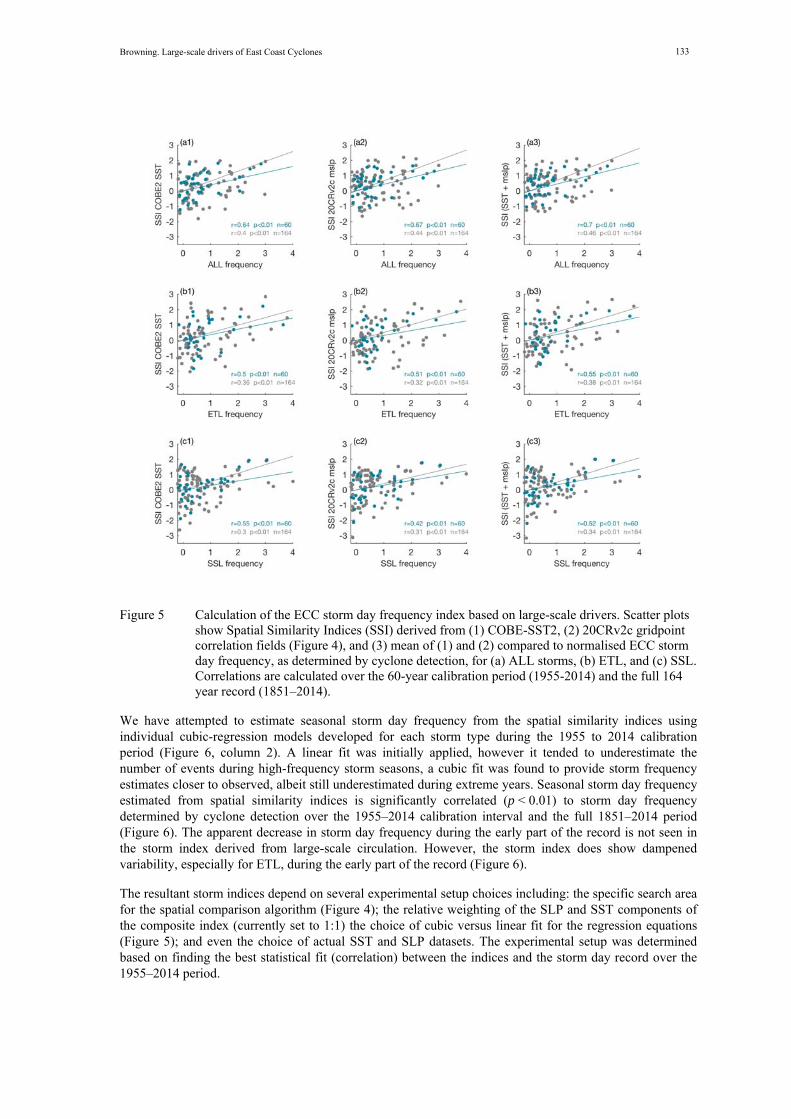
Figure 5 Calculation of the ECC storm day frequency index based on large-scale drivers. Scatter plots show Spatial Similarity Indices (SSI) derived from (1) COBE-SST2, (2) 20CRv2c gridpoint correlation fields (Figure 4), and (3) mean of (1) and (2) compared to normalised ECC storm day frequency, as determined by cyclone detection, for (a) ALL storms, (b) ETL, and (c) SSL. Correlations are calculated over the 60-year calibration period (1955-2014) and the full 164 year record (1851–2014).

We have attempted to estimate seasonal storm day frequency from the spatial similarity indices using individual cubic-regression models developed for each storm type during the 1955 to 2014 calibration period (Figure 6, column 2). A linear fit was initially applied, however it tended to underestimate the number of events during high-frequency storm seasons, a cubic fit was found to provide storm frequency estimates closer to observed, albeit still underestimated during extreme years. Seasonal storm day frequency estimated from spatial similarity indices is significantly correlated (p < 0.01) to storm day frequency determined by cyclone detection over the 1955–2014 calibration interval and the full 1851–2014 period (Figure 6). The apparent decrease in storm day frequency during the early part of the record is not seen in the storm index derived from large-scale circulation. However, the storm index does show dampened variability, especially for ETL, during the early part of the record (Figure 6).

The resultant storm indices depend on several experimental setup choices including: the specific search area for the spatial comparison algorithm (Figure 4); the relative weighting of the SLP and SST components of the composite index (currently set to 1:1) the choice of cubic versus linear fit for the regression equations (Figure 5); and even the choice of actual SST and SLP datasets. The experimental setup was determined based on finding the best statistical fit (correlation) between the indices and the storm day record over the 1955–2014 period.


134

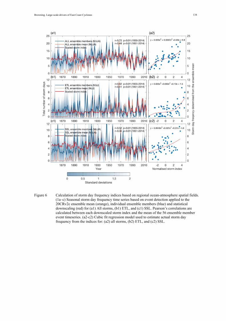
Figure 6 Calculation of storm day frequency indices based on regional ocean-atmosphere spatial fields. (1a–c) Seasonal storm day frequency time series based on event detection applied to the 20CRv2c ensemble mean (orange), individual ensemble members (blue) and statistical downscaling (red) for (a1) All storms, (b1) ETL, and (c1) SSL. Pearson’s correlations are calculated between each downscaled storm index and the mean of the 56 ensemble member event timeseries. (a2-c2) Cubic fit regression model used to estimate actual storm day frequency from the indices for: (a2) all storms, (b2) ETL, and (c2) SSL.


135

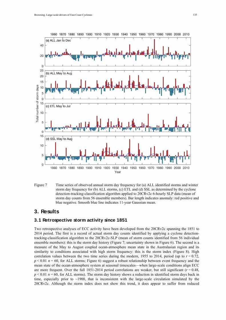
Figure 7 Time series of observed annual storm day frequency for (a) ALL identified storms and winter storm day frequency for (b) ALL storms, (c) ETL and (d) SSL as determined by the cyclone detection-tracking-classification algorithm applied to 20CRv2c 6-hourly SLP data (mean of storm day counts from 56 ensemble members). Bar length indicates anomaly: red positive and blue negative. Smooth blue line indicates 11-year Gaussian mean.

3. Results

3.1 Retrospective storm activity since 1851

Two retrospective analyses of ECC activity have been developed from the 20CRv2c spanning the 1851 to 2014 period. The first is a record of actual storm day counts identified by applying a cyclone detection-tracking-classification algorithm to the 20CRv2c-SLP (mean of storm counts identified from 56 individual ensemble members): this is the storm day history (Figure 7; uncertainty shown in Figure 6). The second is a measure of the May to August coupled ocean-atmosphere mean state in the Australasian region and its similarity to conditions associated with high storm frequency: this is the storm index (Figure 8). High correlation values between the two time series during the modern, 1955 to 2014, period (up to r = 0.72, p < 0.01 n = 60, for ALL storms; Figure 6) suggest a robust relationship between event frequency and the mean state of the ocean-atmosphere system at seasonal timescales—when large-scale conditions align ECC are more frequent. Over the full 1851-2014 period correlations are weaker, but still significant (r = 0.48, p < 0.01 n = 60, for ALL storms). The storm day history shows a reduction in identified storm days back in time, especially prior to ~1900, that is inconsistent with the large-scale circulation simulated by the 20CRv2c. Although the storm index does not show this trend, it does appear to suffer from reduced


136

amplitude; suggesting that neither approach provides a perfect representation of actual ECC activity over the full 1851–2014 period.

3.2 Recent storm day history: 1955–2014

Figure 7 shows both interannual and multidecadal variability in total storm activity with an overall decrease since the mid-1970s. Between 1955–1976 there were an average of 25.9 storm days per year, decreasing to 20.5 per year between 1980–2010. Total winter storm frequency also declined from 1955–1976 (11.4-days per winter) to 1980–2010 (8.3 days per winter). The largest change is seen in SSL with a higher frequency during 1970–1980 (5-days per winter) compared to the recent 1990–-2006 period (3.2-days per winter). ETL, however, were less frequent during the 1970–1980s (1.4-days per winter) than the 1995–2014 period (2.6-days per winter).

Between 1955 and 2014 the stormiest year for all storm types was 1974 due to increased storminess in all seasons, especially summer; two of the stormiest winters were 1956, due to increased SSL activity, and 1967 due to increased ETL activity. During the top 10% of storm seasons (Table A1) the state of the major southern hemisphere climate drivers is broadly consistent with expectations from Table 1. For both ETL and SSL, high activity is usually associated with SOI+ve and warm SST in the eastern tropical Indian Ocean (IOD-ve). High winter ETL activity generally occurs with IPO-ve coupled to SAM+ve while high SSL activity is often coincident with La Niña coupled to IPO-ve and SAM-ve.

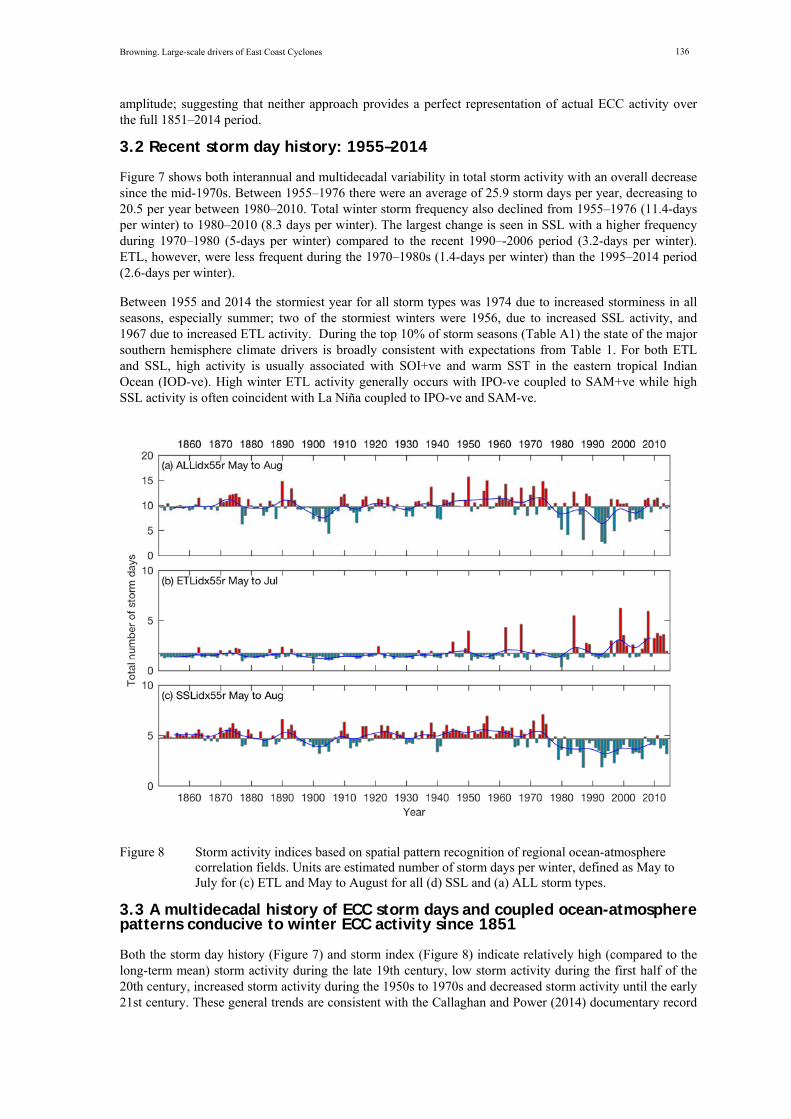
Figure 8 Storm activity indices based on spatial pattern recognition of regional ocean-atmosphere correlation fields. Units are estimated number of storm days per winter, defined as May to July for (c) ETL and May to August for all (d) SSL and (a) ALL storm types.

3.3 A multidecadal history of ECC storm days and coupled ocean-atmosphere patterns conducive to winter ECC activity since 1851

Both the storm day history (Figure 7) and storm index (Figure 8) indicate relatively high (compared to the long-term mean) storm activity during the late 19th century, low storm activity during the first half of the 20th century, increased storm activity during the 1950s to 1970s and decreased storm activity until the early 21st century. These general trends are consistent with the Callaghan and Power (2014) documentary record


137

of storm activity. The late 20th century decline in ECC events appears to be mostly related to a shift away from conditions conducive to extratropical origin SSL, while conditions remained favourable to ETL (Figure 8).

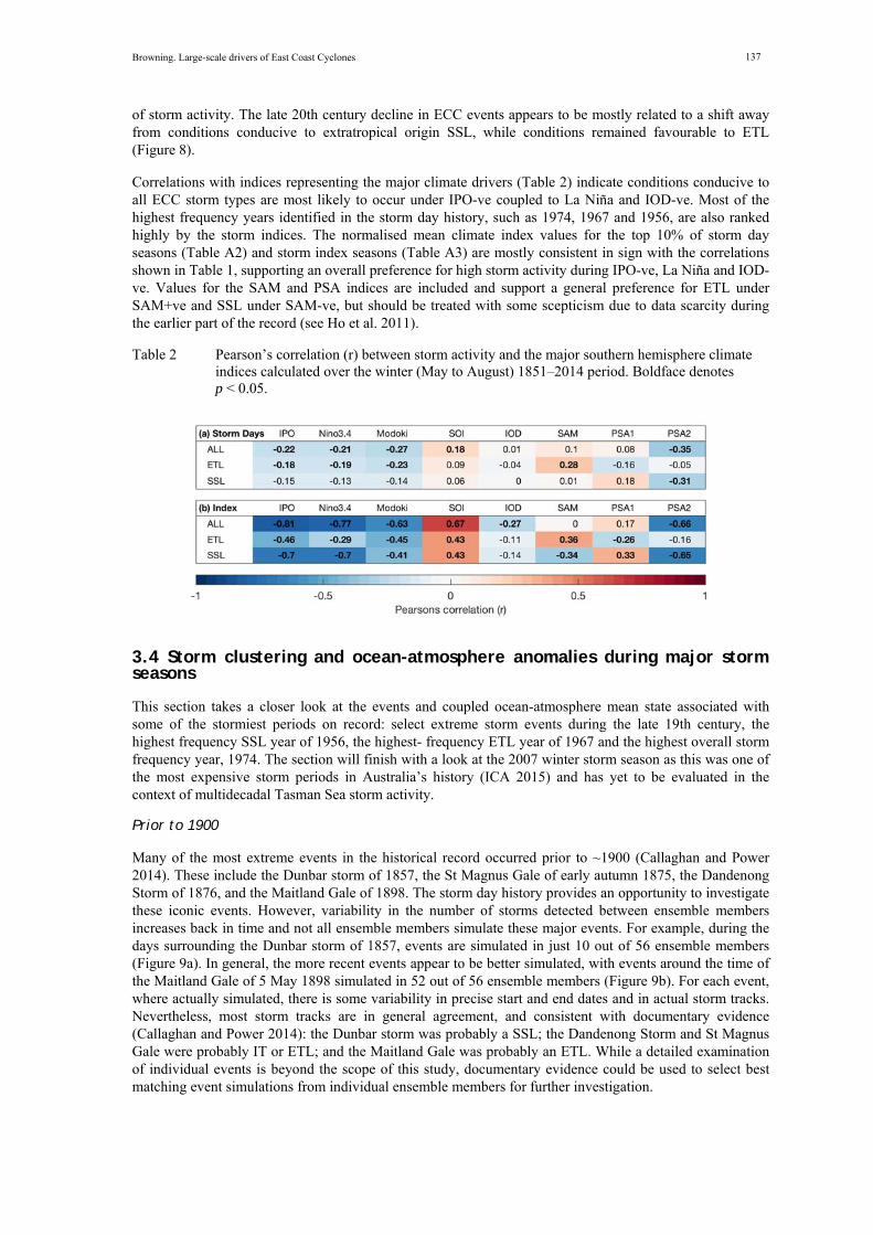
Correlations with indices representing the major climate drivers (Table 2) indicate conditions conducive to all ECC storm types are most likely to occur under IPO-ve coupled to La Niña and IOD-ve. Most of the highest frequency years identified in the storm day history, such as 1974, 1967 and 1956, are also ranked highly by the storm indices. The normalised mean climate index values for the top 10% of storm day seasons (Table A2) and storm index seasons (Table A3) are mostly consistent in sign with the correlations shown in Table 1, supporting an overall preference for high storm activity during IPO-ve, La Niña and IOD-ve. Values for the SAM and PSA indices are included and support a general preference for ETL under SAM+ve and SSL under SAM-ve, but should be treated with some scepticism due to data scarcity during the earlier part of the record (see Ho et al. 2011).

Table 2 Pearson’s correlation (r) between storm activity and the major southern hemisphere climate indices calculated over the winter (May to August) 1851–2014 period. Boldface denotes p < 0.05.

3.4 Storm clustering and ocean-atmosphere anomalies during major storm seasons

This section takes a closer look at the events and coupled ocean-atmosphere mean state associated with some of the stormiest periods on record: select extreme storm events during the late 19th century, the highest frequency SSL year of 1956, the highest- frequency ETL year of 1967 and the highest overall storm frequency year, 1974. The section will finish with a look at the 2007 winter storm season as this was one of the most expensive storm periods in Australia’s history (ICA 2015) and has yet to be evaluated in the context of multidecadal Tasman Sea storm activity.

Prior to 1900

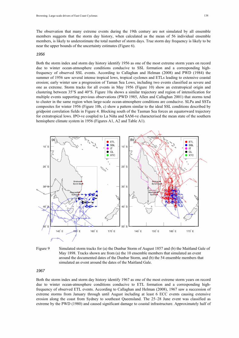
Many of the most extreme events in the historical record occurred prior to ~1900 (Callaghan and Power 2014). These include the Dunbar storm of 1857, the St Magnus Gale of early autumn 1875, the Dandenong Storm of 1876, and the Maitland Gale of 1898. The storm day history provides an opportunity to investigate these iconic events. However, variability in the number of storms detected between ensemble members increases back in time and not all ensemble members simulate these major events. For example, during the days surrounding the Dunbar storm of 1857, events are simulated in just 10 out of 56 ensemble members (Figure 9a). In general, the more recent events appear to be better simulated, with events around the time of the Maitland Gale of 5 May 1898 simulated in 52 out of 56 ensemble members (Figure 9b). For each event, where actually simulated, there is some variability in precise start and end dates and in actual storm tracks. Nevertheless, most storm tracks are in general agreement, and consistent with documentary evidence (Callaghan and Power 2014): the Dunbar storm was probably a SSL; the Dandenong Storm and St Magnus Gale were probably IT or ETL; and the Maitland Gale was probably an ETL. While a detailed examination of individual events is beyond the scope of this study, documentary evidence could be used to select best matching event simulations from individual ensemble members for further investigation.


138

The observation that many extreme events during the 19th century are not simulated by all ensemble members suggests that the storm day history, when calculated as the mean of 56 individual ensemble members, is likely to underestimate the total number of storm days. True storm day frequency is likely to be near the upper bounds of the uncertainty estimates (Figure 6).

1956

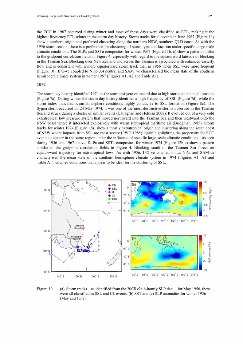
Both the storm index and storm day history identify 1956 as one of the most extreme storm years on record due to winter ocean-atmosphere conditions conducive to SSL formation and a corresponding high-frequency of observed SSL events. According to Callaghan and Helman (2008) and PWD (1984) the summer of 1956 saw several intense tropical lows, tropical cyclones and ETLs leading to extensive coastal erosion; early winter saw a progression of Taman Sea Lows, including two events classified as severe and one as extreme. Storm tracks for all events in May 1956 (Figure 10) show an extratropical origin and clustering between 35°S and 40°S. Figure 10a shows a similar trajectory and region of intensification for multiple events supporting previous observations (PWD 1985, Allen and Callaghan 2001) that storms tend to cluster in the same region when large-scale ocean-atmosphere conditions are conducive. SLPa and SSTa composites for winter 1956 (Figure 10b, c) show a pattern similar to the ideal SSL conditions described by gridpoint correlation fields in Figure 4. Blocking south of the Tasman Sea forces an equatorward trajectory for extratropical lows. IPO-ve coupled to La Niña and SAM-ve characterised the mean state of the southern hemisphere climate system in 1956 (Figures A1, A2 and Table A1).

Figure 9 Simulated storm tracks for (a) the Dunbar Storm of August 1857 and (b) the Maitland Gale of May 1898. Tracks shown are from (a) the 10 ensemble members that simulated an event around the documented dates of the Dunbar Storm, and (b) the 54 ensemble members that simulated an event around the dates of the Maitland Gale.

1967

Both the storm index and storm day history identify 1967 as one of the most extreme storm years on record due to winter ocean-atmosphere conditions conducive to ETL formation and a corresponding high-frequency of observed ETL events. According to Callaghan and Helman (2008), 1967 saw a succession of extreme storms from January through until August including at least 6 ECC events causing extensive erosion along the coast from Sydney to southeast Queensland. The 25–28 June event was classified as extreme by the PWD (1980) and caused significant damage to coastal infrastructure. Approximately half of


139

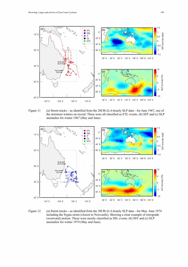
the ECC in 1967 occurred during winter and most of these days were classified as ETL, making it the highest frequency ETL winter in the storm day history. Storm tracks for all events in June 1967 (Figure 11) show a northern origin and preferred clustering along the northern NSW, southern QLD coast. As with the 1956 storm season, there is a preference for clustering of storm type and location under specific large-scale climatic conditions. The SLPa and SSTa composites for winter 1967 (Figure 11b, c) show a pattern similar to the gridpoint correlation fields in Figure 4, especially with regard to the equatorward latitude of blocking in the Tasman Sea. Blocking over New Zealand and across the Tasman is associated with enhanced easterly flow and is consistent with a more equatorward storm track than in 1956 when SSL were more frequent (Figure 10). IPO-ve coupled to Niño 3.4 neutral and SAM+ve characterised the mean state of the southern hemisphere climate system in winter 1967 (Figures A1, A2 and Table A1).

1974

The storm day history identified 1974 as the stormiest year on record due to high storm counts in all seasons (Figure 7a). During winter the storm day history identifies a high frequency of SSL (Figure 7d), while the storm index indicates ocean-atmosphere conditions highly conducive to SSL formation (Figure 8c). The Sygna storm occurred on 24 May 1974, it was one of the most destructive storms observed in the Tasman Sea and struck during a cluster of similar events (Callaghan and Helman 2008). It evolved out of a very cold extratropical low pressure system that moved northward into the Tasman Sea and then westward onto the NSW coast where it interacted explosively with warm subtropical maritime air (Bridgman 1985). Storm tracks for winter 1974 (Figure 12a) show a mostly extratropical origin and clustering along the south coast of NSW where impacts from SSL are most severe (PWD 1985); again highlighting the propensity for ECC events to cluster in the same region under the influence of specific large-scale climatic conditions—as seen during 1956 and 1967 above. SLPa and SSTa composites for winter 1974 (Figure 12b-c) show a pattern similar to the gridpoint correlation fields in Figure 4. Blocking south of the Tasman Sea forces an equatorward trajectory for extratropical lows. As with 1956, IPO-ve coupled to La Niña and SAM-ve characterised the mean state of the southern hemisphere climate system in 1974 (Figures A1, A2 and Table A1), coupled conditions that appear to be ideal for the clustering of SSL.

Figure 10 (a) Storm tracks—as identified from the 20CRv2c 6-hourly SLP data—for May 1956, these were all classified as SSL and CL events. (b) SST and (c) SLP anomalies for winter 1956 (May and June).


140

Figure 11 (a) Storm tracks—as identified from the 20CRv2c 6-hourly SLP data—for June 1967, one of the stormiest winters on record. These were all classified as ETL events. (b) SST and (c) SLP anomalies for winter 1967 (May and June).

Figure 12 (a) Storm tracks—as identified from the 20CRv2c 6-hourly SLP data—for May–June 1974 including the Sygna storm (closest to Newcastle). Showing a clear example of retrograde (westward) motion. These were mostly classified as SSL events. (b) SST and (c) SLP anomalies for winter 1974 (May and June).


141

The Pasha Bulka storm of 2007

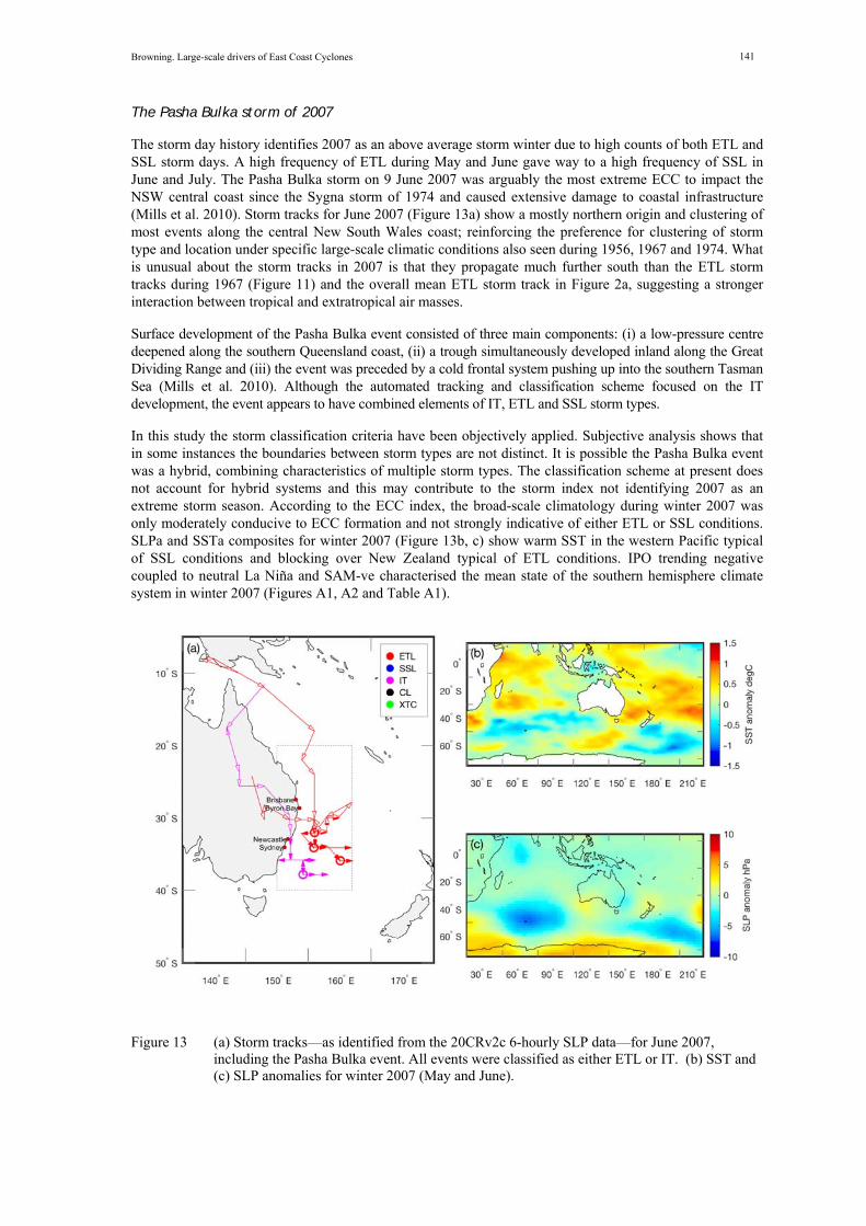
The storm day history identifies 2007 as an above average storm winter due to high counts of both ETL and SSL storm days. A high frequency of ETL during May and June gave way to a high frequency of SSL in June and July. The Pasha Bulka storm on 9 June 2007 was arguably the most extreme ECC to impact the NSW central coast since the Sygna storm of 1974 and caused extensive damage to coastal infrastructure (Mills et al. 2010). Storm tracks for June 2007 (Figure 13a) show a mostly northern origin and clustering of most events along the central New South Wales coast; reinforcing the preference for clustering of storm type and location under specific large-scale climatic conditions also seen during 1956, 1967 and 1974. What is unusual about the storm tracks in 2007 is that they propagate much further south than the ETL storm tracks during 1967 (Figure 11) and the overall mean ETL storm track in Figure 2a, suggesting a stronger interaction between tropical and extratropical air masses.

Surface development of the Pasha Bulka event consisted of three main components: (i) a low-pressure centre deepened along the southern Queensland coast, (ii) a trough simultaneously developed inland along the Great Dividing Range and (iii) the event was preceded by a cold frontal system pushing up into the southern Tasman Sea (Mills et al. 2010). Although the automated tracking and classification scheme focused on the IT development, the event appears to have combined elements of IT, ETL and SSL storm types.

In this study the storm classification criteria have been objectively applied. Subjective analysis shows that in some instances the boundaries between storm types are not distinct. It is possible the Pasha Bulka event was a hybrid, combining characteristics of multiple storm types. The classification scheme at present does not account for hybrid systems and this may contribute to the storm index not identifying 2007 as an extreme storm season. According to the ECC index, the broad-scale climatology during winter 2007 was only moderately conducive to ECC formation and not strongly indicative of either ETL or SSL conditions. SLPa and SSTa composites for winter 2007 (Figure 13b, c) show warm SST in the western Pacific typical of SSL conditions and blocking over New Zealand typical of ETL conditions. IPO trending negative coupled to neutral La Niña and SAM-ve characterised the mean state of the southern hemisphere climate system in winter 2007 (Figures A1, A2 and Table A1).

Figure 13 (a) Storm tracks—as identified from the 20CRv2c 6-hourly SLP data—for June 2007, including the Pasha Bulka event. All events were classified as either ETL or IT. (b) SST and (c) SLP anomalies for winter 2007 (May and June).


142

4. Discussion

4.1 Large-scale influences on ECC formation during the 20th century

The stormiest years in recent history (since 1955): 1956 (SSL), 1967 (ETL) and 1974 (ALL storms) display distinct clustering of storm types, tracks and regions of maximum intensification during the early winter period. The latitude of blocking in the Tasman appears to be a deterministic factor on the type and location of ECC. Persistent blocking south of the Tasman, such as during 1956 and 1974, is conducive to frequent SSL events while blocking in the central Tasman, such as during 1967, is associated with ETL events. The location of blocking in the Tasman is locally influenced by the land-sea temperature difference (Lamb 1959, Carleton 1979, Mo et al. 1987) and remotely influenced by large-scale Rossby wave forcing (Coughlan 1983, Karoly 1983, Renwick and Revell 1999). Poleward propagating barotropic Rossby waves can be generated by tropical convective anomalies (these may or may not be ENSO related); their influence on mid-latitude blocking is dependent on the state of the SAM (e.g. Stammerjohn et al. 2008, Cai et al. 2011b). Therefore, blocking variability in the Tasman is subject to the complex interaction of both local and remote tropical and extratropical drivers (Kidson 2000, Jiang 2011, Jiang et al. 2013). This combination of factors may help to explain why we see only moderate to weak linear correlations between storm frequency and ENSO, IPO and SAM. However, extreme (top 10%) storm years do show a distinct preference for formation during IPO-ve coupled to La Niña; SAM-ve is more likely to be associated with SSL, while SAM+ve is more likely to be associated with ETL (Table A1).

Both the 1967 ETL season and the recent 2007 storm season both occurred during IPO trending toward its negative phase. Hopkins and Holland (1997) put forward a hypothesis that ETL events were more frequent during the transition from El Niño to La Niña mean state as defined by the difference in the SOI value from year-1 to year+1. No such relationship is observed between the SOI and ETL or SSL frequency (using the storm day dataset) over the period used by Hopkins and Holland (1997) (1955–1992) or the longer 1955 to 2014 period. However, there is a weak positive correlation between the trend in the IPO and the ETL observational record (r = 0.28, p < 0.05, n = 55) and the ETL index (r = 0.34, p < 0.01, n = 138). Where the trend in the IPO is calculated over the May to July period as the difference between year-1 and year-0 (similar but weaker correlations were achieved calculating the difference between year-1 and year+1). Although the correlations are relatively weak—albeit statistically significant—most major storm periods do seem to correspond to shifts from IPO positive to IPO negative including 1960, 1967, 1984, 1999 and 2007. The ETL index also indicates a shift in the IPO for 8 of the top 10 storm years between 1851 and 2014. Over a time period longer than Hopkins and Holland (1998), this study does not support their findings with regard to the SOI (in terms of the correlations values); however, it does support the concept that most high-frequency ETL seasons do tend to occur during a shift in the mean state of the Pacific from ‘El Niño like’ to ‘La Niña like’, as defined by the IPO. SSL frequency on the other hand is not related to a shift in the IPO, rather SSL frequency is moderately correlated to the IPO where SSL events and climatic conditions conducive to SSL events are more frequent during IPO-ve.

4.2 Downscaling and the link between weather and climate

The rationale for downscaling the seasonal 20CRv2c data to estimate cyclone activity is based on the dynamical relationship between seasonal mean climate state and the formation of individual events (Lorrey et al. 2007). There is persistence within the climate system such that large-scale features like the Subtropical Ridge (Drosdowsky 2005, Cai et al. 2011a) and mid-latitude blocking (Pook et al. 2013, Ummenhofer et al. 2013) establish in preferred locations over seasonal timescales and influence the behaviour of synoptic weather and storm tracks (Baines 1983, Jiang et al. 2013). Browning and Goodwin (2013) showed that ECC event frequency and storm type are guided by large-scale (coupled ocean-atmosphere) influences at seasonal timescales. Therefore, an understanding of the seasonal mean state can be effectively used to infer variability in actual synoptic scale weather events. Significant correlations between individually tailored indices representing the state of the coupled ocean-atmosphere system and actual ECC event counts (Figures 5 and 6) over the 1955 to 2014 period support the use of spatial pattern recognition as a downscaling tool. The alternative approach of Dowdy et al. (2013) uses upper atmospheric geostrophic vorticity to estimate ECL probability from the ERA-Interim. This is a potentially useful approach for high-resolution GCM simulations with realistic upper atmospheres, however it cannot discriminate between storm types and is not suitable for application to coarser resolution datasets such as the 20CRv2c that are based only on surface observations.


143

4.3 The issue of storm intensity

One important issue not investigated here is storm intensity. There appears to be a relationship between documentary evidence of extreme events and high-frequency storm seasons (see 1956, 1967, 1974 and 2007 above); suggesting that when large-scale conditions are conducive, events are both more frequent and extreme. Accurately defining intensity is quiet challenging. SLP gradients provide some indication, however the reanalysis data may be too coarse to provide precise measurements. Impacts based storm definitions have been used by Hopkins and Holland (1997) and Shand et al. (2011), but these rely on accurate measurements of variables such as precipitation, wind strength and wave height that can be extremely localised. Developing an accurate objective measure of storm intensity is an ongoing area of research.

4.4 Findings are strongly dependent on data quality

Any conclusions about storm variability based on retrospective storm histories and indices are strongly dependent upon the realism of the data from which they are derived. Data scarcity remains the biggest issue when developing any long climate history in the southern hemisphere—prior to 1948 and south of 50°S, there are only 10 stations or less included in the 20CRv2c (Figure 1). Storm day counts determined by cyclone detection appear to underestimate storm activity during the early part of the record. Determining storm day frequency from individual ensemble members, as opposed to the ensemble mean, goes some way towards addressing this issue; however, there are still considerable uncertainties during the 19th century.

ECC indices derived from the large-scale circulation provides a realistic estimate of storm activity during the mid-to-late 20th century, when the 20CRv2c is well constrained by observational data. However, underestimation of ECC variability—especially during the 19th century—suggest that the downscaling approach is also affected by observational data deficiencies. Unfortunately, it is difficult to assess the reality of large-scale circulation during the early decades of the 20CRv2c. For example, Pohl et al. (2012) conducted an in-depth comparison between SAM indices derived from 20CR, HadSLP2 and the Marshall (2003) and Visbeck (2009) SAMs, confirming poor agreement between all indices prior to the 1950s. Therefore, conclusions about past storm activity, whether derived from cyclone identification or large-scale indices, should be supplemented by comparison with documentary evidence and proxy climate data if available.

5. Conclusion

The major conclusions with regard to ECC are that during high-frequency storm seasons there is clear clustering of storm types based on storm track and latitude of maximum intensification. The primary determinant on this appears to be the latitude of blocking in the Tasman Sea. Blocking is influenced by multiple local and remote factors; this is likely the main reason for only moderate to weak linear correlations with indices representing the major climate drivers. However, by looking at seasonal variability in storm day frequency and regional climate conditions, it appears the highest storm activity periods do occur under IPO-ve coupled to La Niña, when there is an overall negative SLP anomaly in the Australian region and warmer (more energetic) SST in the western Pacific. This is consistent with Power and Callaghan (2015) who found a strong association between ECL frequency and La Niña since 1876. SSL originating in the extratropics are more likely when blocking is poleward under SAM-ve, while ETL originating in the subtropical easterlies are more likely when blocking is equatorward under SAM+ve. Anomalous years with conditions conducive to both storm types may promote hybrid systems: it is possible that the 2007 Pasha Bulka storm was one such event. These events appear to display the strongest retrograde motion (westward) during intensification and warrant further investigation.

One of the main objectives of this research has been concerned with developing a suitable approach to estimate storm activity from imperfect data. While automated cyclone detection algorithms provide a record of actual ECC events, data scarcity appears to affect the simulation of individual cyclones during the early part of the 20CRv2c. However, seasonal event frequency can be estimated by downscaling using individually tailored indices based on spatial recognition of coupled ocean-atmosphere variability. When applied to the 20CRv2c, this approach produces storm indices that are highly correlated to the observational record and show that large-scale circulation during the early years of the 20CRv2c is indicative of higher storm activity than is actually simulated. Unfortunately, at present there is no way to validate the accuracy of the early portion of the 20CRv2c at high-latitudes, so conclusions must be viewed with regard to this


144

important caveat. The downscaling approach is readily adaptable to any clearly definable storm type and should be applicable to other gridded climate datasets, such as existing Climate Model Intercomparison Project (CMIP5) simulations (Taylor et al. 2011) and proxy-based reanalyses (Browning 2014).

Acknowledgements

This research contributes to the Australian Eastern Seaboard Climate Change Initiative and was in part funded by a Macquarie University External Collaborative Grant with the New South Wales Office for Environment and Heritage, and the New South Wales Environmental Trust. S.A. Browning received a postgraduate Macquarie University Research Scholarship (MQRES). Support for the Twentieth Century Reanalysis Project dataset is provided by the U.S. Department of Energy, Office of Science Innovative and Novel Computational Impact on Theory and Experiment (DOE INCITE) program, and Office of Biological and Environmental Research (BER), and by the National Oceanic and Atmospheric Administration Climate Program Office. We thank Jeff Callaghan and an anonymous reviewer for their constructive comments.

References

Allen, J.T., Pezza, A.B. and Black, M.T. 2010. Explosive cyclogenesis: a global climatology comparing multiple reanalyses. J. Climate, 23, 6468–6484, doi:10.1175/2010JCLI3437.1.

Bridgman, H.A. 1985. The Sygna storm at Newcastle – 12 years later. Meteorology Australia, VBP 4574, 10–16.

Bromwich, D.H. and Fogt, R.L. 2004. Strong trends in the skill of the ERA-40 and NCEP–NCAR reanalyses in the high and mid-latitudes of the southern hemisphere, 1958–2001*. J. Climate, 17, 4603–4619, doi:10.1175/3241.1.

Browning, S.A. and Goodwin, I.D. 2013. Large-scale influences on the evolution of winter subtropical maritime cyclones affecting Australia’s east coast. Mon. Weather Rev, 141, 2416–2431, doi:10.1175/MWR-D-12-00312.1.

Browning, S. 2014: The Drivers Of Multidecadal Climate Variability In The Extratropics Over The Late Holocene, Ph.D. thesis. Macquarie University.

Callaghan, J. and Helman, P. 2008. Severe Storms on the east coast of Australia 1770–2008. Griffith Centre for Coastal Management, Griffith University, Gold Coast, Queensland, 252 pp.

Callaghan, J. and Power. S.B. 2014: Major coastal flooding in southeastern Australia 1860–2012, associated deaths and weather systems. Austr Meteorol Oceanogr J. 64, 183–213

Caron, L.-P., Jones, C.G. and Winger, K. 2011. Impact of resolution and downscaling technique in simulating recent Atlantic tropical cylone activity. Clim. Dynam, 37, 869–892, doi:10.1007/s00382-010-0846-7.

Compo, G.P., Whitaker, J.S., Sardeshmukh, P.D., Matsui, N., Allan, R.J., Yin, X., Gleason, B.E., Vose, R. S., Rutledge, G., Bessemoulin, P., Brönnimann, S., Brunet, M., Crouthamel, R.I., Grant, A.N., Groisman, P.Y., Jones, P.D., Kruk, M.C., Kruger, A.C., Marshall, G.J., Maugeri, M., Mok, H.Y., Nordli, Ø., Ross, T.F., Trigo, R.M., Wang, X.L., Woodruff, S.D. and Worley, S.J. 2011. The twentieth century reanalysis project. Q. J. Roy. Meteor. Soc, 137, 1–28, doi:10.1002/qj.776.

Daloz, A.S., Chauvin, F., Walsh, K., Lavender, S., Abbs, D. and Roux, F. 2012. The ability of general circulation models to simulate tropical cyclones and their precursors over the North Atlantic main development region. Clim. Dynam, 39, 1559–1576, doi:10.1007/s00382-012-1290-7.

Dee, D.P., Uppala, S.M., Simmons, A.J., Berrisford, P., Poli, P., Kobayashi, S., Andrae, U., Balmaseda, M. A., Balsamo, G., Bauer, P., Bechtold, P., Beljaars, A.C.M., van de Berg, L., Bidlot, J., Bormann, N., Delsol, C., Dragani, R., Fuentes, M., Geer, A.J., Haimberger, L., Healy, S. B., Hersbach, H., Hólm, E. V., Isaksen, L., Kållberg, P., Köhler, M., Matricardi, M., McNally, A.P., Monge-Sanz, B.M., Morcrette, J.J., Park, B.K., Peubey, C., de Rosnay, P., Tavolato, C., Thépaut, J.N. and Vitart, F. 2011. The ERA-Interim reanalysis: configuration and performance of the data assimilation system. Q. J. Roy. Meteor. Soc., 137, 553–597, doi:10.1002/qj.828.

Dowdy, A.J., Mills, G.A. and Timbal, B. 2013. Large‐scale diagnostics of extratropical cyclogenesis in eastern Australia. Int. J. Climatol, 33, 2318–2327, doi:10.1002/joc.3599.

Elison Timm, O., Takahashi, M., Giambelluca, T.W. and Diaz, H.F. 2013. On the relation between large‐scale circulation pattern and heavy rain events over the Hawaiian Islands: Recent trends and future changes. Journal of Geophysical Research-Atmospheres, 118, 4129–4141, doi:10.1002/jgrd.50314.

Emanuel, K. 2010. Tropical cyclone activity downscaled from NOAA-CIRES Reanalysis, 1908–1958. J. Adv. Model. Earth Syst, 2, 1, doi:10.3894/JAMES.2010.2.1.


145

Emanuel, K., Sundererejan, R. and Williams, J. 2008. Hurricanes and Global Warming: Results from Downscaling IPCC AR4 Simulations. B. Am. Meteor. Soc, 89, 347–367, doi:10.1175/BAMS-89-3-347.

Folland, C.K., Renwick, J.A. Salinger, M.J. and Mullan, A.B. 2002. Relative influences of the Interdecadal Pacific Oscillation and ENSO on the South Pacific Convergence Zone. Geophys. Res. Lett, 29, 1643, doi:10.1029/2001GL014201.

Grose, M.R., Pook, M.J., Mcintosh, P.C., Risbey, J.S. and Bindoff, N.L. 2012. The simulation of cutoff lows in a regional climate model: reliability and future trends. Clim. Dynam, 39, 445–459, doi:10.1007/s00382-012-1368-2.

Henley, B.J., Gergis, J., Karoly, D.J. Power, S. Kennedy, J. and Folland, C.K. 2015. A Tripole Index for the Interdecadal Pacific Oscillation. Clim. Dynam, doi:10.1007/s00382-015-2525-1.

Hines, K.M., Bromwich, D.H. and Marshall, G.J. 2000. Artificial surface pressure trends in the NCEP-NCAR reanalysis over the Southern Ocean and Antarctica*. J. Climate, 13, 3940–3952, doi:10.1175/1520-0442(2000)013<3940:ASPTIT>2.0.CO;2.

Hirahara, S., Ishii, M. and Fukuda, Y. 2014: Centennial-scale sea surface temperature analysis and its uncertainty. J. Climate, 27, 57–75, doi:10.1175/JCLI-D-12-00837.1.

Hunt, B.G. and Watterson, I.G. 2010. The temporal and spatial characteristics of surrogate tropical cyclones from a multi-millenial simulation. Clim. Dynam, 34, 699–718, doi:10.1007/s00382-009-0627-3.

Jones, D.A. and Simmonds, I. 1993. A climatology of southern hemisphere extratropical cyclones. Clim. Dynam, 9, 131–145, doi:10.1007/BF00209750.

Kalnay, E., Kanamitsu, M., Kistler, R., Collins, W., Deaven, D., Gandin, L., Iredell, M., Saha, S., White, G., Woollen, J., Zhu, Y., Leetmaa, A., Reynolds, R., Chelliah, M., Ebisuzaki, W., Higgins, W., Janowiak, J., Mo, K.C., Ropelewski, C., Wang, J., Jenne, R. and Joseph, D. 1996. The NCEP/NCAR 40-Year Reanalysis Project. B. Am. Meteor. Soc, 77, 437–471, doi:10.1175/1520-0477(1996)077<0437:TNYRP>2.0.CO;2.

Katzfey, J.J. and McInnes, K.L. 1996. GCM simulations of eastern Australian cutoff lows. J. Climate, 9, 2337–2355, doi:10.1175/1520-0442(1996)009<2337:GSOEAC>2.0.CO;2.

Leroy, A. and Wheeler, M.C. 2008. Statistical prediction of weekly tropical cyclone activity in the southern hemisphere. Mon. Weather Rev, 136, 3637–3654, doi:10.1175/2008MWR2426.1.

Mills, G.A., Webb, R., Davidson, N.E., Kepert, J., Seed, A. and Abbs, D.2010. The Pasha Bulker east coast low of 8 June 2007. CAWCR Technical Report No. 023, 74 pp.

Murray, R. and Simmonds, I. 1991. A numerical scheme for tracking cyclone centres from digital data Part I: development and operation of. Australian Meteorological Magazine, 39, 155–166.

Pepler, A.S., Di Luca, A., Ji, F., Alexander, L.V., Evans, J.P. and Sherwood, S.C. 2015. Impact of Identification Method on the Inferred Characteristics and Variability of Australian East Coast Lows. Mon. Weather Rev, 143, 864–877, doi:10.1175/MWR-D-14-00188.1.

Pielke, R.A. and Wilby, R.L. 2012. Regional climate downscaling: What's the point? Eos Trans. AGU, 93, 52–53.

Power, S.B. and Callaghan, J. 2015: Variability in severe coastal flooding in south-eastern Australia since the mid-19th century, associated storms and death tolls. J. Appl. Meteor. Climatol, JAMC–D–15–0146.1, doi:10.1175/JAMC-D-15-0146.1.

Public Works Department (PWD). 1985. Elevated coastal levels; Storms affecting N.S.W. coast 1880-1980. Weatherex Meteorological Services and Public Works Department Rep. 85041, 574 pp.

Ramsay, H.A., Leslie, L.M., Lamb, P.J., Richman, M.B. and Leplastrier, M. 2008. Interannual Variability of Tropical Cyclones in the Australian Region: Role of Large-Scale Environment. J. Climate, 21, 1083–1103, doi:10.1175/2007JCLI1970.1.

Wang, X.L., Feng, Y., Compo, G.P., Swail, V.R., Zwiers, F.W., Allan, R.J. and Sardeshmukh, P.D. 2013. Trends and low frequency variability of extra-tropical cyclone activity in the ensemble of twentieth century reanalysis. Clim. Dynam, 40, 2775–2800, doi:10.1007/s00382-012-1450-9.


146

Appendix

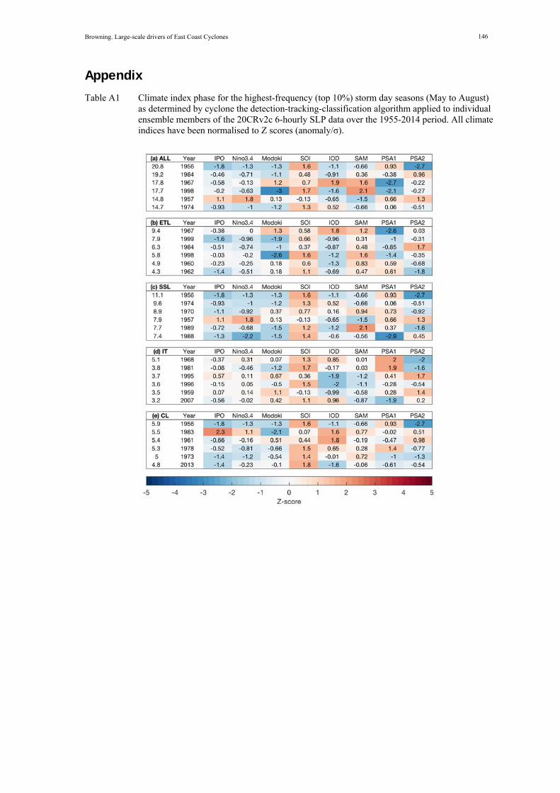
Table A1 Climate index phase for the highest-frequency (top 10%) storm day seasons (May to August) as determined by cyclone the detection-tracking-classification algorithm applied to individual ensemble members of the 20CRv2c 6-hourly SLP data over the 1955-2014 period. All climate indices have been normalised to Z scores (anomaly/σ).


147

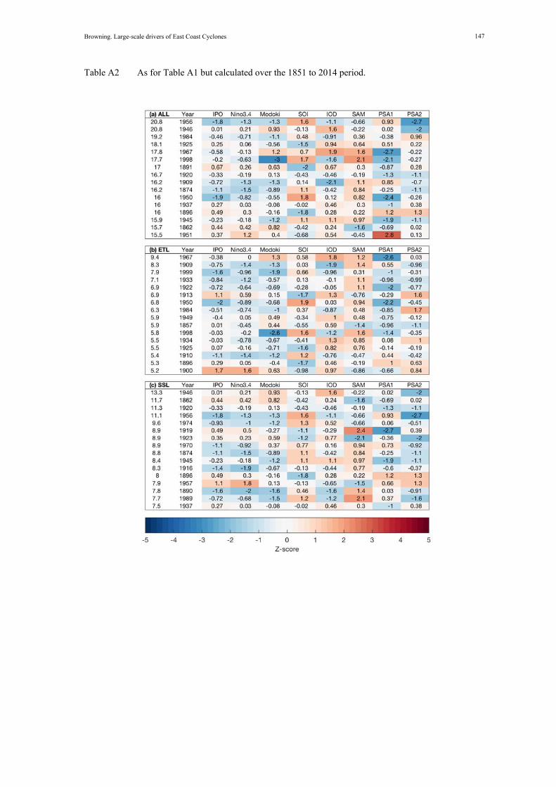
Table A2 As for Table A1 but calculated over the 1851 to 2014 period.


148

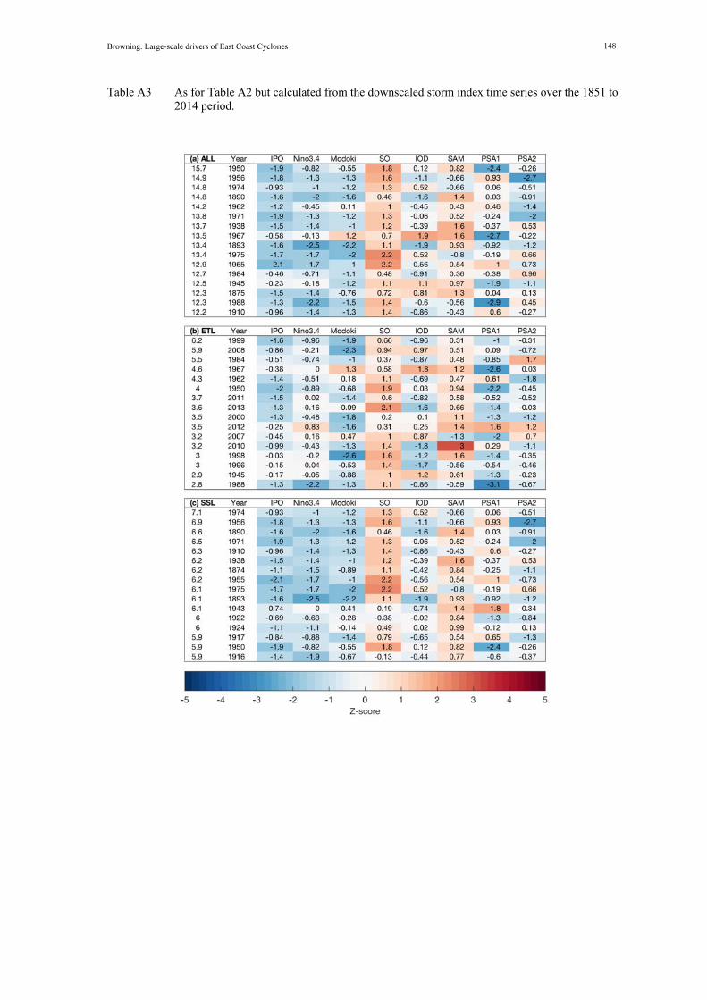
Table A3 As for Table A2 but calculated from the downscaled storm index time series over the 1851 to 2014 period.


149

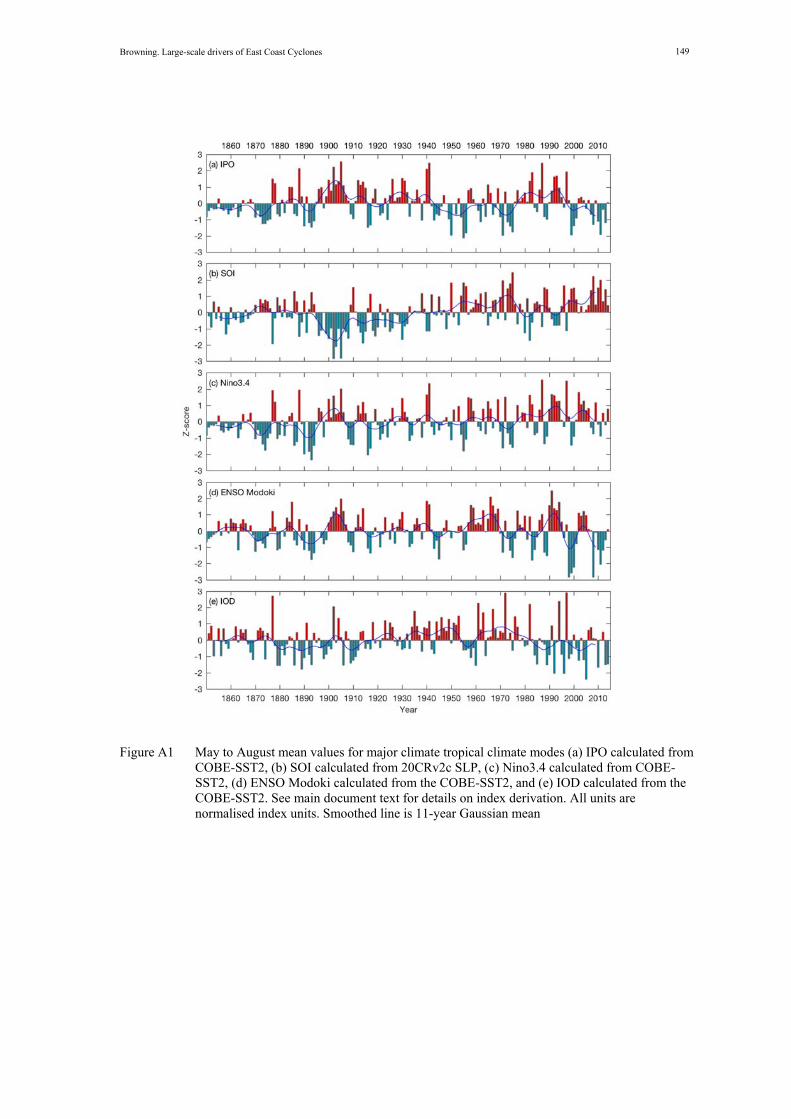
Figure A1 May to August mean values for major climate tropical climate modes (a) IPO calculated from COBE-SST2, (b) SOI calculated from 20CRv2c SLP, (c) Nino3.4 calculated from COBE-SST2, (d) ENSO Modoki calculated from the COBE-SST2, and (e) IOD calculated from the COBE-SST2. See main document text for details on index derivation. All units are normalised index units. Smoothed line is 11-year Gaussian mean


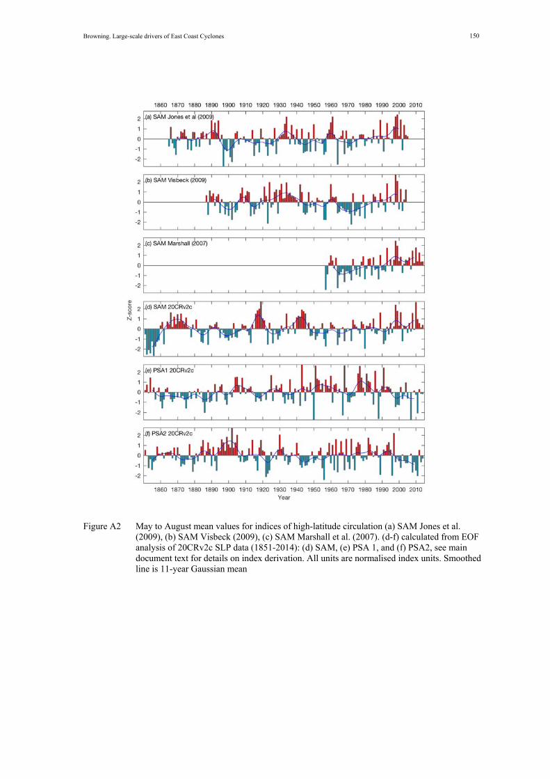
150

Figure A2 May to August mean values for indices of high-latitude circulation (a) SAM Jones et al. (2009), (b) SAM Visbeck (2009), (c) SAM Marshall et al. (2007). (d-f) calculated from EOF analysis of 20CRv2c SLP data (1851-2014): (d) SAM, (e) PSA 1, and (f) PSA2, see main document text for details on index derivation. All units are normalised index units. Smoothed line is 11-year Gaussian mean

large-scale drivers of australian east coast cyclones since 1851 · corresponding author: stuart...

Documents