large margin semi-supervised learning - journal of machine

Journal of Machine Learning Research 8 (2007) 1867-1891 Submitted 2/06; Revised 1/07; Published 8/07

Large Margin Semi-supervised Learning

Junhui Wang [email protected]

Xiaotong Shen [email protected]

School of StatisticsUniversity of MinnesotaMinneapolis, MN 55455, USA

Editor: Tommi Jaakkola

Abstract

In classification, semi-supervised learning occurs when a large amount of unlabeled data is avail-able with only a small number of labeled data. In such a situation, how to enhance predictabilityof classification through unlabeled data is the focus. In this article, we introduce a novel largemargin semi-supervised learning methodology, using grouping information from unlabeled data,together with the concept of margins, in a form of regularization controlling the interplay betweenlabeled and unlabeled data. Based on this methodology, we develop two specific machines in-volving support vector machines and ψ-learning, denoted as SSVM and SPSI, through differenceconvex programming. In addition, we estimate the generalization error using both labeled andunlabeled data, for tuning regularizers. Finally, our theoretical and numerical analyses indicatethat the proposed methodology achieves the desired objective of delivering high performance ingeneralization, particularly against some strong performers.

Keywords: generalization, grouping, sequential quadratic programming, support vectors

1. Introduction

In many classification problems, a large amount of unlabeled data is available, while it is costly toobtain labeled data. In text categorization, particularly web-page classification, a machine is trainedwith a small number of manually labeled texts (web-pages), as well as a huge amount of unlabeledtexts (web-pages), because manually labeling is impractical; compare with Joachims (1999). Inspam detection, a small group of identified e-mails, spam or non-spam, is used, in conjunction witha large number of unidentified e-mails, to train a filter to flag incoming spam e-mails, comparewith Amini and Gallinari (2003). In face recognition, a classifier is trained to recognize faces withscarce identified and enormous unidentified faces, compare with Balcan et al. (2005). In a situationas such, one research problem is how to enhance accuracy of prediction in classification by usingboth unlabeled and labeled data. The problem of this sort is referred to as semi-supervised learning,which differs from a conventional “missing data” problem in that the size of unlabeled data greatlyexceeds that of labeled data, and missing occurs only in response. The central issue that this articleaddresses is how to use information from unlabeled data to enhance predictability of classification.

In semi-supervised learning, a sample {Zi = (Xi,Yi)}nli=1 is observed with labeling Yi ∈ {−1,1},

in addition to an independent unlabeled sample {X j}nj=nl+1 with n = nl +nu, where Xk = (Xk1, · · · ,

Xkp); k = 1, · · · ,n is an p-dimensional input. Here the labeled sample is independently and iden-tically distributed according to an unknown joint distribution P(x,y), and the unlabeled sample is

c©2007 Junhui Wang and Xiaotong Shen.

WANG AND SHEN

independently and identically distributed from distribution P(x) that may not be the marginal distri-bution of P(x,y).

A number of semi-supervised learning methods have been proposed through some assumptionsrelating P(x) to the conditional distribution P(Y = 1|X = x). These methods include, among others,co-training (Blum and Mitchell, 1998), the EM method (Nigam, McCallum, Thrun and Mitchell,1998), the bootstrap method (Collins and Singer, 1999), information-based regularization (Szummerand Jaakkola, 2002), Bayesian network (Cozman, Cohen and Cirelo, 2003), Gaussian random fields(Zhu, Ghahramani and Lafferty, 2003), manifold regularization (Belkin, Niyogi and Sindhwani,2004), and discriminative-generative models (Ando and Zhang, 2004). Transductive SVM (TSVM;Vapnik, 1998) uses the concept of margins.

Despite progress, many open problems remain. Essentially all existing methods make variousassumptions about the relationship between P(Y = 1|X = x) and P(x) in a way for an improvementto occur when unlabeled data is used. Note that an improvement of classification may not be ex-pected when simply imputing labels of X through an estimated P(Y = 1|X = x) from labeled data,compare with Zhang and Oles (2000). In other words, the potential gain in classification stemsfrom an assumption, which is usually not verifiable or satisfiable in practice. As a consequence, anydeparture from such an assumption is likely to degrade the “alleged” improvement, and may yieldworse performance than classification with labeled data alone.

The primary objective of this article is to develop a large margin semi-supervised learningmethodology to deliver high performance of classification by using unlabeled data. The method-ology is designed to adapt to a variety of situations by identifying as opposed to specifying a rela-tionship between labeled and unlabeled data from data. It yields an improvement when unlabeleddata can reconstruct the optimal classification boundary, and yields a no worse performance than itssupervised counterpart otherwise. This is in contrast to the existing methods.

Through three key ingredients, our objective is achieved, including (1) comparing all possiblegrouping boundaries from unlabeled data for classification, (2) using labeled data to determinelabel assignment for classification as well as a modification of the grouping boundary, and (3)interplay between (1) and (2) through tuning to connect grouping to classification for seeking thebest classification boundary. These ingredients are integrated in a form of regularization involvingthree regularizers, each controlling classification with labeled data, grouping with unlabeled data,and interplay between them. Moreover, we introduce a tuning method using unlabeled data fortuning the regularizers.

Through the proposed methodology and difference convex programming, we develop two spe-cific machines based on support vector machines (SVM; Cortes and Vapnik, 1995) and ψ-learning(Shen, Tseng, Zhang and Wong, 2003), denoted as SSVM and SPSI. Numerical analysis indicatesthat SSVM and SPSI achieve the desired objective, particularly against TSVM and a graphicalmethod in simulated and benchmark examples. Moreover, a novel learning theory is developed toquantify SPSI’s generalization error as a function of complexity of the class of candidate decisionfunctions, the sample sizes (nl,nu), and the regularizers. To our knowledge, this is the first attemptto relate a classifier’s generalization error to (nl,nu) and regularizers in semisupervised learning.This theory not only explains SPSI’s performance, but also supports our aforementioned discus-sion concerning the interplay between grouping and classification, as evident from Section 5 thatSPSI can recover the optimal classification performance at a speed in nu because of grouping fromunlabeled data.

1868

LARGE MARGIN SEMI-SUPERVISED LEARNING

This article is organized in eight sections. Section 2 introduces the proposed semi-supervisedlearning methodology. Section 3 treats non-convex minimization through difference convex pro-gramming. Section 4 proposes a tuning methodology that uses both labeled and unlabeled data toenhance of accuracy of estimation of the generalization error. Section 5 presents some numerical ex-amples, followed by a novel statistical learning theory in Section 6. Section 7 contains a discussion,and the appendix is devoted to technical proofs.

2. Methodology

In this section, we present our proposed margin-based semi-supervised learning method as well itsconnection to other existing popular methodologies.

2.1 Proposed Methodology

We begin with our discussion in linear margin classification with labeled data (Xi,Yi)nli=1 alone.

Given a class of linear decision functions of the form f (x) = wTf x+w f ,0 ≡ (1,xT )w f , a cost function

C ∑nli=1 L(yi f (xi))+J( f ) is minimized with respect to f ∈F , a class of candidate decision functions,

to obtain the minimizer f yielding a classifier Sign( f ), where J( f ) = ‖w f ‖2/2 is the reciprocal ofthe L2 geometric margin, and L(·) is a margin loss defined by functional margins zi = yi f (xi);i = 1, · · · ,nl .

Different learning methodologies are defined by different margin losses. Margin losses include,among others, the hinge loss L(z) = (1− z)+ for SVM with its variants L(z) = (1− z)q

+ for q >1; compare with Lin (2002); the ρ-hinge loss L(z) = (ρ− z)+ for nu-SVM (Scholkopf, Smola,Williamson and Bartlett, 2000) with ρ > 0 to be optimized; the ψ-loss L(z) = ψ(z), with ψ(z) =1−Sign(z) if z ≥ 1 or z < 0, and 2(1− z) otherwise, compare with Shen et al. (2003), the logisticloss L(z) = log(1+e−z), compare with Zhu and Hastie (2005); the sigmoid loss L(z) = 1− tanh(cz);compare with Mason, Baxter, Bartlett and Frean (2000). A margin loss L(z) is said to be a largemargin if L(z) is nonincreasing in z, which penalizes small margin values.

In order to extract useful information about classification from unlabeled data, we construct aloss U(·) for a grouping decision function g(x) = (1,xT )wg ≡ wT

g x+wg,0, with Sign(g(x)) indicatinggrouping. Towards this end, we let U(z) = min{y=±1} L(yz) by minimizing y in L(·) to remove itsdependency of y. As shown in Lemma 1, U(z) = L(|z|), which is symmetric in z and indicates thatit can only determine the grouping boundary that occurs near in an area with low value of U(z) butprovide no information regarding labeling.

While U can be used to extract the grouping boundary, it needs to yield the Bayes decisionfunction f ∗ = argmin f∈F EL(Y f (X)) in order for it to be useful for classification, where E is theexpectation with respect to (X ,Y ). More specifically, it needs f ∗ = argming∈F EU(g(X)). How-ever, it does not hold generally since argming∈F EU(g(X)) can be any g ∈ F satisfying |g(x)| ≥ 1.Generally speaking, U gives no information about labeling Y . To overcome this difficulty, we reg-ularize U and introduce our regularized loss for semi-supervised learning to induce a relationshipbetween classification f and grouping g:

S( f ,g;C) = C1L(y f (x))+C2U(g(x))+C3

2‖w f −wg‖2 +

12‖wg‖2, (1)

where C = (C1,C2,C3) are non-negative regularizers, and ‖w f −wg‖2 = ‖w f −wg‖2 +(w f ,0−wg,0)2

is the usual L2-Euclidean norm in Rp+1. Whereas L(y f (x)) regularizes the contribution from labeled

1869

WANG AND SHEN

data, U(g(x)) controls the information extracted from unlabeled data, and ‖w f −wg‖2 penalizes thedisagreement between f and g, specifying a loose relationship between f and g. The interrelationbetween f and g is illustrated in Figure 3. Note that in (1) the geometric margin 2

‖w f ‖2 does not enter

as it is regularized implicitly through 2‖w f−wg‖2 and 2

‖wg‖2 .

In nonlinear learning, a kernel K(·, ·) that maps from S×S to R 1 is usually introduced for flex-ible representations: f (x) = (1,K(x,x1), · · · ,K(x,xn))w f and g(x) = (1,K(x,x1), · · · ,K(x,xn))wg

with w f = (w f ,w f ,0) and wg = wg +wg,0. Then nonlinear surfaces separate instances of two classes,implicitly defined by K(·, ·), where the reproducing kernel Hilbert spaces (RKHS) plays an impor-tant role; compare with Wahba (1990) and Gu (2000). The forgoing treatment for the linear case isapplicable when the Euclidean inner product 〈xi,x j〉 is replaced by K(xi,x j). In this sense, the linearcase may be regarded as a special case of nonlinear learning.

Lemma 1 says that the regularized loss (1) allows U to yield precise information about theBayes decision function f ∗ when after tuning. Specifically, U targets at the Bayes decision functionin classification when C1 and C3 are large, and grouping can differ from classification at other Cvalues.

Lemma 1 For any large margin loss L(z), U(z) = miny∈{−1,1} L(yz) = L(|z|), where y = Sign(z) =argminy∈{−1,1} L(yz) for any given z. Additionally,

( f ∗C,g∗C) = arg inff ,g∈F

ES( f ,g;C) → ( f ∗, f ∗) as C1,C3 → ∞.

In the case that ( f ∗C,g∗C) is not unique, we choose it as any minimizer of ES( f ,g;C).Through (1), we propose our cost function for semi-supervised learning:

s( f ,g) = C1

nl

∑i=1

L(yi f (xi))+C2

n

∑j=nl+1

U(g(x j))+C3

2‖ f −g‖2 +

12‖g‖2

−, (2)

where in the linear case, ‖g‖− = ‖wg‖ and ‖ f − g‖ = ‖w f −wg‖; in the nonlinear case ‖g‖2− =

wTg Kwg, ‖ f −g‖2 = (w f −wg)

T K(w f −wg)+(w f ,0−wg,0)2 is the RKHS norm, with an n×n matrix

K whose i jth element is K(xi,x j). Minimization of (2) with respect to ( f ,g) yields an estimateddecision function f thus classifier Sign( f ). The constrained version of (2), after introducing slackvariables {ξk ≥ 0;k = 1, · · · ,n}, becomes

C1

nl

∑i=1

ξi +C2

n

∑j=nl+1

ξ j +C3

2‖ f −g‖2 +

12‖g‖2

−, (3)

subject to ξi −L(yi f (xi)) ≥ 0; i = 1, · · · ,nl; ξ j −U(g(x j)) ≥ 0; j = nl + 1, · · · ,n. Minimization of(2) with respect to ( f ,g), equivalently, minimization of (3) with respect to ( f ,g,ξk;k = 1, · · · ,n)subject to the constraints gives our estimated decision function ( f , g), where f is for classification.

Two specific machines SSVM and SPSI will be further developed in what follows. In (2), SSVMuses L(z) = (1− z)+ and U(z) = (1−|z|)+, and SPSI uses L(z) = ψ(z) and U(z) = 2(1−|z|)+.

2.2 Connection Between SSVM and TSVM

To better understand the proposed methodology, we now explore the connection between SSVMand TSVM. In specific, TSVM uses a cost function in the form of

C1

nl

∑i=1

(1− yi f (xi))+ +C2

n

∑j=nl+1

(1− y j f (x j))+ +12‖ f‖2

−,

1870


where minimization with respect to (y j : j = nl +1, · · · ,n; f ) yields the estimated decision functionf . It can be thought of as the limiting case of SSVM as C3 → ∞ forcing f = g in (2).

SSVM in (3) stems from grouping and interplay between grouping and classification, whereasTSVM focuses on classification. Placing TSVM in the framework of SSVM, we see that SSVMrelaxes TSVM in that it allows grouping (g) and classification (f) to differ, whereas f ≡ g for TSVM.Such a relaxation yields that |e( f , f ∗)| = |GE( f )−GE( f ∗)| is bounded by |e( f , g)|+ |e(g,g∗C)|+|e(g∗C, f ∗)|, with |e( f , g)| controlled by C3, the estimation error |e(g,g∗C)| controlled by C2n−1

u andthe approximation error |e(g∗C, f ∗)| controlled by C1 and C3. As a result, all these error terms can bereduced simultaneously with a suitable choice of (C1,C2,C3), thus delivering better generalization.This aspect will be demonstrated by our theory in Section 6 and numerical analysis in Section 5. Incontrast, TSVM is unable to do so, and needs to increase the size of one error in order to reducethe other error, and vice versa, compare with Wang, Shen and Pan (2007). This aspect will be alsoconfirmed by our numerical results.

The forgoing discussion concerning SSVM is applicable to (2) with a different large margin lossL as well.

3. Non-convex Minimization Through Difference Convex Programming

Optimization in (2) involves non-convex minimization, because of non-convex U(z) and/or possi-bly L(z) in z. On the basis of recent advances in global optimization, particularly difference convex(DC) programming, we develop our minimization technique. Key to DC programming is decompo-sition of our cost function into a difference of two convex functions, based on which iterative upperapproximations can be constructed to yield a sequence of solutions converging to a stationary point,possibly an ε-global minimizer. This technique is called DC algorithms (DCA; An and Tao, 1997),permitting a treatment of large-scale non-convex minimization.

To use DCA for SVM and ψ-learning in (2), we construct DC decompositions of the cost func-tions of SPSI and SSVM sψ and sSV M in (2):

sψ = sψ1 − sψ

2 ; sSV M = sSV M1 − sSV M

2 ,

where L(z) = ψ(z) and U(z) = 2(1−|z|)+ for SPSI,

sψ1 = C1 ∑nl

i=1 ψ1(yi f (xi))+C2 ∑nj=nl+1 2U1(g(x j))+ C3

2 ‖ f −g‖2 + 12‖g‖2

−,

sψ2 = C1 ∑nl

i=1 ψ2(yi f (xi))+C2 ∑nj=nl+1 2U2(g(x j));

and L(z) = (1− z)+ and U(z) = (1−|z|)+ for SSVM,

sSV M1 = C1 ∑nl

i=1(1− yi f (xi))+ +C2 ∑nj=nl+1U1(g(x j))+ C3

2 ‖ f −g‖2 + 12‖g‖2

−,

sSV M2 = C2 ∑n

j=nl+1U2(g(x j)).

These DC decompositions are obtained through DC decompositions of (1−|z|)+ = U1(z)−U2(z)and ψ(z) = ψ1(z)−ψ2(z), where U1 = (|z|−1)+, U2 = |z|−1, ψ1 = 2(1− z)+, and ψ2 = 2(−z)+.The decompositions are displayed in Figure 1.

With these decompositions, we treat the nonconvex minimization in (2) by solving a sequenceof quadratic programming (QP) problems. Algorithm 1 solves (2) for SPSI and SSVM.Algorithm 1: (Sequential QP)Step 1. (Initialization) Set initial values f (0) = g(0) as the solution of SVM with labeled data alone,

1871

WANG AND SHEN

−3 −2 −1 0 1 2 3

−1.

0−

0.5

0.0

0.5

1.0

1.5

2.0

z

UU1

U2

−1.5 −1.0 −0.5 0.0 0.5 1.0 1.5

01

23

45

z

ψψ1

ψ2

Figure 1: The left panel is a plot of U , U1 and U2, for the DC decomposition of U = U1−U2. Solid,dotted and dashed lines represent U , U1 and U2, respectively. The right panel is a plot ofψ, ψ1 and ψ2, for the DC decomposition of ψ = ψ1 −ψ2. Solid, dotted and dashed linesrepresent ψ, ψ1 and ψ2, respectively.

and an precision tolerance level ε > 0.Step 2. (Iteration) At iteration k + 1, compute ( f (k+1),g(k+1)) by solving the corresponding dualproblems given in (4).Step 3. (Stopping rule) Terminate when |s( f (k+1),g(k+1))− s( f (k),g(k))| ≤ ε.Then the estimate ( f , g) is the best solution among ( f (l),g(l))k+1

l=1 .At iteration k + 1, after omitting constants that are independent of (4), the primal problems are

required to solve

minw f ,wg

sψ1 ( f ,g)−〈( f ,g),∇sψ

2 ( f (k),g(k))〉,

minw f ,wg

sSV M1 ( f ,g)−〈( f ,g),∇sSVM

2 ( f (k),g(k))〉. (4)

Here ∇sSV M2 = (∇SV M

1 f ,∇SV M2 f ,∇SVM

1g ,∇SV M2g ) is the gradient vector of sSV M

2 with respect to ( f ,g),

with ∇SV M1g = C2 ∑n

j=nl+1 ∇U2(g(x j))x j, ∇SV M2g = C2 ∑n

j=nl+1 ∇U2(g(x j)), ∇SV M1 f = 0p, and ∇SV M

2 f = 0,

where ∇U2(z) = 1 if z > 0, and ∇U2(z) = −1 otherwise. Similarly, ∇sψ2 = (∇ψ

1 f ,∇ψ2 f ,∇

ψ1g,∇

ψ2g)

is the gradient vector of sψ2 with respect to (w f ,wg), with ∇ψ

1 f = C1 ∑nli=1 ∇ψ2(yi f (xi))yixi, ∇ψ

2 f =

C1 ∑nli=1 ∇ψ2(yi f (xi))yi, ∇ψ

1g = 2∇SV M1g , and ∇ψ

2g = 2∇SV M2g , where ∇ψ2(z) = 0 if z > 0 and ∇ψ2(z) =

−2 otherwise. By Karush-Kuhn-Tucker(KKT)’s condition, the primal problems in (4) are equivalentto their dual forms, which are generally easier to work with and given in the Appendix C.

By Theorem 3 of Liu, Shen and Wong (2005), limk→∞

‖ f (k+1) − f (∞)‖ = 0 for some f (∞), and con-

vergence of Algorithm 1 is superlinear in that limk→∞

‖ f (k+1) − f (∞)‖/‖ f (k) − f (∞)‖ = 0 and

limk→∞

‖g(k+1) − g(∞)‖/‖g(k) − g(∞)‖ = 0, if there does not exist an instance x such that f (∞)(x) =

g(∞)(x) = 0 with f (∞)(x) = (1,K(x,x1), · · · ,K(x,xn))w(∞)f and g(∞)(x) = (1,K(x,x1), · · · ,

K(x,xn))w(∞)g . Therefore, the number of iterations required for Algorithm 1 is o(log(1/ε)) to

achieve the precision ε > 0.

1872


4. Tuning Involving Unlabeled Data

This section proposes a novel tuning method based on the concept of generalized degrees of freedom(GDF) and the technique of data perturbation (Shen and Huang, 2006; Wang and Shen, 2006),through both labeled and unlabeled data. This permits tuning of three regularizers C = (C1,C2,C3)in (2) to achieve the optimal performance.

The generalization error (GE) of a classification function f is defined as GE( f ) = P(Y f (X) <0) = EI(Y 6= Sign( f (X))), where I(·) is the indicator function. The GE( f ) usually depends on theunknown truth, and needs to be estimated. Minimization of the estimated GE( f ) with respect to therange of the regularizers gives the optimal regularization parameters.

For tuning, write f as fC, and write (X l,Y l) = (Xi,Yi)nli=1 and Xu = {X j}n

j=nl+1. By Theorem 1

of Wang and Shen (2006), the optimal estimated GE( fC), after ignoring the terms independent offC, has the form of

EGE( fC)+1

2nl

nl

∑i=1

Cov(Yi,Sign( fC(Xi))|X l)+14

D1(Xl, fC). (5)

Here, EGE( fC) = 12nl

∑nli=1(1−Yi Sign( fC(Xi))) is the training error, and D1(X l, fC) = E

(E(4(X))−

1nl

∑nli=14(Xi)|X l

)with 4(X) = (E(Y |X)− Sign( fC(X)))2, where E(·|X) and E(·|X l) are condi-

tional expectations with respect to Y and Y l respectively. As illustrated in Wang and Shen (2006),the estimated (5) based on GDF is optimal in the sense that it performs no worse than the methodof cross-validation and other tuning methods; see Efron (2004).

In (5), Cov(Yi,Sign( fC(Xi))|X l); i = 1 · · · ,nl and D1(X l, fC) need to be estimated. It appearsthat Cov(Yi,Sign( fC(Xi))|X l) is estimated only through labeled data, for which we apply the dataperturbation technique of Wang and Shen (2006). On the other hand, D1(X l, fC) is estimated directlythrough (X l,Y l) and Xu jointly.

Our method proceeds as follows. First generate pseudo data Y ∗i by perturbing Yi:

Y ∗i =

{Yi with probability 1− τ,Yi with probability τ,

(6)

where 0 < τ < 1 is the size of perturbation, and (Yi + 1)/2 is sampled from a Bernoulli distribu-tion with p(xi), an rough probability estimate of p(xi) = P(Y = 1|X = xi), which may be obtainedthrough the same classification method that defines fC or through logistic regression when it doesn’tyield an estimated p(x), such as SVM and ψ-learning. The estimated covariance is proposed to be

Cov(Yi,Sign( fC(Xi))|X l) =1

k(Yi, p(Xi))Cov∗(Y ∗

i ,Sign( f ∗C(Xi))|X l); i = 1, · · · ,nl, (7)

where k(Yi, p(Xi)) = τ + τ(1− τ) ((Yi+1)/2−p(Xi))2

p(Xi)(1−p(Xi)), and f ∗C is an estimated decision function through

the same classification method trained through (Xi,Y ∗i )nl

i=1.

To estimate D1, we express it as a difference between the true model error E(E(Y |X)−Sign( fC(X)))2 and its empirical version n−1

l ∑nli=1(E(Yi|Xi)−Sign( fC(Xi)))

2, where the former can

1873

WANG AND SHEN

be estimated through (X l,Y l) and Xu. The estimated D1 becomes

D1(Xl, fC) = E∗

(1nu

n

∑j=nl+1

((2p(X j)−1)−Sign( f ∗C(X j)))2−

1nl

nl

∑i=1

((2p(Xi)−1)−Sign( f ∗C(Xi)))2

∣∣∣∣∣Xl

),

(8)

Generally, Cov in (7) and D1 in (8) can be always computed using a Monte Carlo (MC) ap-proximation of Cov∗, E∗, when it is difficult to obtain their analytic forms. Specifically, when Y l isperturbed D times, a MC approximation of Cov and D1 can be derived:

Cov(Yi,Sign( fC(Xi))|X l) ≈ 1D−1

D

∑d=1

1k(Yi, p(Xi))

Sign( f ∗dC (Xi))(Y

∗di −Y

∗i ), (9)

D1(Xl, fC) ≈ 1

D−1

D

∑d=1

(1nu

n

∑j=nl+1

((2p(X j)−1)−Sign( f ∗dC (X j)))

2−

1nl

nl

∑i=1

((2p(Xi)−1)−Sign( f ∗dC (Xi)))

2

),

where Y ∗di ;d = 1, · · · ,D are perturbed samples according to (6), Y

∗i = 1

D ∑d Y ∗di , and f ∗d

C is trained

through (Xi,Y ∗di )nl

i=1. Our proposed estimate GE becomes

GE( fC) = EGE( fC)+1

2nl

nl

∑i=1

Cov(Yi,Sign( fC(Xi))|X l)+14

D1(Xl, fC), (10)

By the law of large numbers, GE converges to (5) as D → ∞. In practice, we recommend D to beat least nl to ensure the precision of MC approximation and τ to be 0.5. In contrast to the estimatedGE with labeled data alone, the GE( fC) in (10) requires no perturbation of X when X u is available.This permits more robust and computationally efficient estimation.

Minimization of (10) with respect to C yields the minimizer C, which is optimal in terms of GEas suggested by Theorem 2, under similar technical assumptions as in Wang and Shen (2006).

(C.1): (Loss and risk) limnl→∞ supC |GE( fC)/E(GE( fC))−1| = 0 in probability.(C.2): (Consistency of initial estimates) For almost all x, pi(x)→ pi(x), as nl → ∞; i = 1, · · · ,nl .(C.3): (Positivity) Assume that inf

CE(GE( fC)) > 0.

Theorem 2 Under Conditions C.1-C.3, limnl ,nu→∞

(lim

τ→0+GE( fC)/ inf

CGE( fC)

)= 1.

Theorem 2 says the ideal optimal performance infC GE( fC) can be realized by GE( fC) whenτ → 0+ and nl ,nu → ∞ against any other tuning method.

1874


5. Numerical Examples

This section examines effectiveness of SSVM and SPSI and compare them against SVM with la-beled data alone, TSVM and a graphical method of Zhu, Ghahramani and Lafferty (2003), in bothsimulated and benchmark examples. A test error, averaged over 100 independent replications, isused to measure their performances.

For simulation comparison, we define the amount of improvement of a method over SVM withlabeled data alone as the percent of improvement in terms of the Bayesian regret,

(T (SV M)−T (Bayes))− (T (·)−T (Bayes))T (SV M)−T (Bayes)

, (11)

where T (·) and T (Bayes) are the test error of any method and the Bayes error. This metric seemsto be sensible, which is against the baseline—the Bayes error T (Bayes), which is approximated bythe test error over a test sample of large size, say 105.

For benchmark comparison, we define the amount of improvement over SVM as

T (SV M)−T (·)T (SV M)

, (12)

which underestimates the amount of improvement in absence of the Bayes rule.Numerical analyses are performed in R2.1.1. For TSVM, SVMlight (Joachims, 1999) is used.

For the graphical method, a MATLAB code provided in Zhu, Ghahramani and Lafferty (2003) is

employed. In the linear case, K(s, t) = 〈s, t〉; in the Gaussian kernel case, K(s, t) = exp(− ‖s−t‖2

σ2

),

where σ2 is set to be p, a default value in the “svm” routine of R, to reduce computational cost fortuning σ2.

5.1 Simulations and Benchmarks

Two simulated and three benchmark examples are examined. In each example, we perform a gridsearch to minimize the test error of each classifier with respect to tuning parameters, in order toeliminate the dependency of the classifier on these parameters. Specifically, one regularizer forSVM and one tuning parameter σ in the Gaussian weight matrix for the graphical method, tworegularization regularizers for TSVM, and three regularizers for SSVM and SPSI are optimizedover [10−2,103]. For SSVM and SPSI, C is searched through a set of unbalanced grid points,based on our small study of the relative importance among (C1,C2,C3). As suggested by Figure2, C3 appears to be most crucial to GE( fC), whereas C2 is less important than (C1,C3), and C1

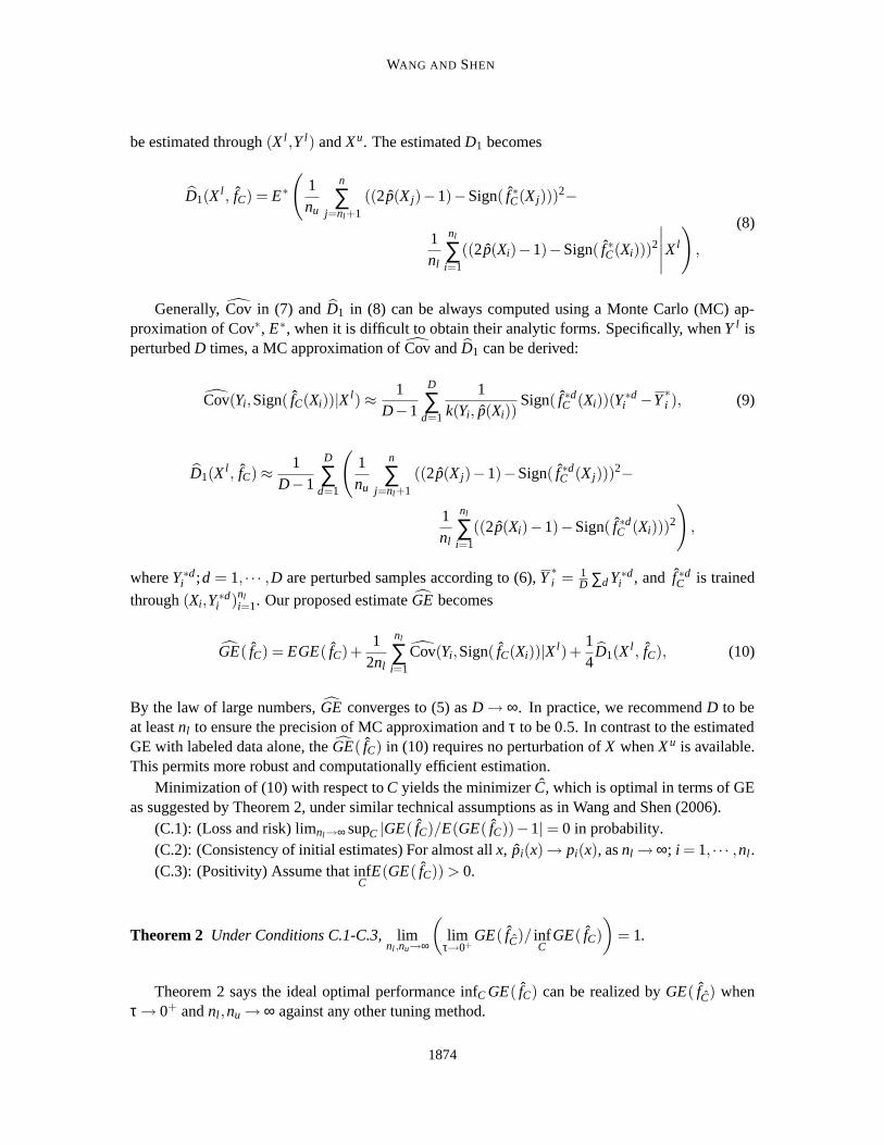
is only useful when its value is not too large. This leads to our unbalanced search over C, thatis, C1 ∈ {10−2,10−1,1,10,102}, C2 ∈ {10−2,1,102}, and C3 ∈ {10m/4;m = −8,−7, · · · ,12}. Thisstrategy seems reasonable as suggested by our simulation. Clearly, a more refined search is expectedto yield better performance for SSVM and SPSI.

Example 1: A random sample {(Xi1,Xi2,Yi); i = 1, · · · ,1000} is generated as follows. First,1000 independent instances (Yi,Xi1,Xi2) are sampled according to (Yi +1)/2∼Bernoulli(0.5), Xi1 ∼Normal(Yi,1), and Xi2 ∼ Normal(0,1). Second, 200 instances are randomly selected for training,and the remaining 800 instances are retained for testing. Next, 190 unlabeled instances (Xi1,Xi2)are obtained by removing labels from a randomly chosen subset of the training sample, whereas theremaining 10 instances are treated as labeled data. The Bayes error is 0.162.

1875

WANG AND SHEN

C2

C1

GE

C3

C2

GE

C3

C1

GE

Figure 2: Plot of GE( fC) as a function of (C1,C2,C3) for one random selected sample of theWBC example. The top left, the top right and the bottom left are plots of GE( fC)versus (C1,C2), (C2,C3) and (C3,C1), respectively. Here (C1,C2,C3) take values in set{10−2+m/4;m = 0,1, · · · ,20}.

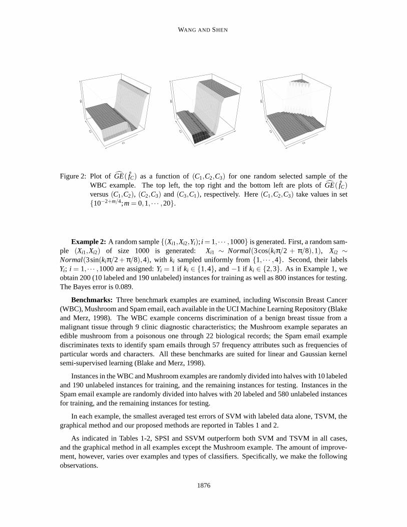
Example 2: A random sample {(Xi1,Xi2,Yi); i = 1, · · · ,1000} is generated. First, a random sam-ple (Xi1,Xi2) of size 1000 is generated: Xi1 ∼ Normal(3cos(kiπ/2 + π/8),1), Xi2 ∼Normal(3sin(kiπ/2 + π/8),4), with ki sampled uniformly from {1, · · · ,4}. Second, their labelsYi; i = 1, · · · ,1000 are assigned: Yi = 1 if ki ∈ {1,4}, and −1 if ki ∈ {2,3}. As in Example 1, weobtain 200 (10 labeled and 190 unlabeled) instances for training as well as 800 instances for testing.The Bayes error is 0.089.

Benchmarks: Three benchmark examples are examined, including Wisconsin Breast Cancer(WBC), Mushroom and Spam email, each available in the UCI Machine Learning Repository (Blakeand Merz, 1998). The WBC example concerns discrimination of a benign breast tissue from amalignant tissue through 9 clinic diagnostic characteristics; the Mushroom example separates anedible mushroom from a poisonous one through 22 biological records; the Spam email examplediscriminates texts to identify spam emails through 57 frequency attributes such as frequencies ofparticular words and characters. All these benchmarks are suited for linear and Gaussian kernelsemi-supervised learning (Blake and Merz, 1998).

Instances in the WBC and Mushroom examples are randomly divided into halves with 10 labeledand 190 unlabeled instances for training, and the remaining instances for testing. Instances in theSpam email example are randomly divided into halves with 20 labeled and 580 unlabeled instancesfor training, and the remaining instances for testing.

In each example, the smallest averaged test errors of SVM with labeled data alone, TSVM, thegraphical method and our proposed methods are reported in Tables 1 and 2.

As indicated in Tables 1-2, SPSI and SSVM outperform both SVM and TSVM in all cases,and the graphical method in all examples except the Mushroom example. The amount of improve-ment, however, varies over examples and types of classifiers. Specifically, we make the followingobservations.

1876


Data Method SVMl TSVM Graph SSVM SPSI SVMc

n×dim Improv. Improv. Improv. Improv.Example 1 Linear .344(.0104) .249(.0134) .188(.0084) .184(.0084) .164(.0084)1000×2 52.2% .232(.0108) 85.7% 87.9%

Gaussian .385(.0099) .267(.0132) 61.5% .201(.0072) .200(.0069) .196(.0015)52.9% 82.5% 83.0%

Example 2 Linear .333(.0129) .222(.0128) .129(.0031) .128(.0031) .115(.0032)1000×2 45.5% .213(.0114) 83.6% 84.0%

Gaussian .347(.0119) .258(.0157) 49.2% .175(.0092) .175(.0098) .151(.0021)34.5% 66.7% 66.7%

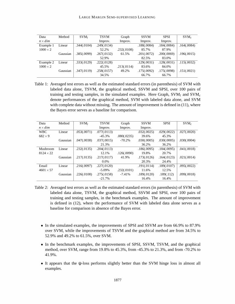
Table 1: Averaged test errors as well as the estimated standard errors (in parenthesis) of SVM withlabeled data alone, TSVM, the graphical method, SSVM and SPSI, over 100 pairs oftraining and testing samples, in the simulated examples. Here Graph, SVMl and SVMc

denote performances of the graphical method, SVM with labeled data alone, and SVMwith complete data without missing. The amount of improvement is defined in (11), wherethe Bayes error serves as a baseline for comparison.


n×dim Improv. Improv. Improv.WBC Linear .053(.0071) .077(.0113) .032(.0025) .029(.0022) .027(.0020)682×9 -45.3% .080(.0235) 39.6% 45.3%

Gaussian .047(.0038) .037(.0015) -70.2% .030(.0005) .030(.0005) .030(.0004)21.3% 36.2% 36.2%

Mushroom Linear .232(.0135) .204(.0113) .186(.0095) .184(.0095) .041(.0018)8124×22 12.1% .126(.0090) 19.8% 20.7%

Gaussian .217(.0135) .217(.0117) 41.9% .173(.0126) .164(.0123) .021(.0014)0.0% 20.3% 24.4%

Email Linear .216(.0097) .227(.0120) .191(.0114) .189(.0107) .095(.0022)4601×57 -5.09% .232(.0101) 11.6% 12.5%

Gaussian .226(.0108) .275(.0158) -7.41% .189(.0120) .189(.112) .099(.0018)-21.7% 16.4% 16.4%

Table 2: Averaged test errors as well as the estimated standard errors (in parenthesis) of SVM withlabeled data alone, TSVM, the graphical method, SSVM and SPSI, over 100 pairs oftraining and testing samples, in the benchmark examples. The amount of improvementis defined in (12), where the performance of SVM with labeled data alone serves as abaseline for comparison in absence of the Bayes error.

• In the simulated examples, the improvements of SPSI and SSVM are from 66.9% to 87.9%over SVM, while the improvements of TSVM and the graphical method are from 34.5% to52.9% and 49.2% to 61.5%, over SVM.

• In the benchmark examples, the improvements of SPSI, SSVM, TSVM, and the graphicalmethod, over SVM, range from 19.8% to 45.3%, from -45.3% to 21.3%, and from -70.2% to41.9%.

• It appears that the ψ-loss performs slightly better than the SVM hinge loss in almost allexamples.

1877

WANG AND SHEN

• SPSI and SSVM nearly reconstruct all relevant information about labeling in the two simu-lated examples and the WBC example, when they are compared with SVM with full labeldata. This suggests that room for further improvement in these cases is small.

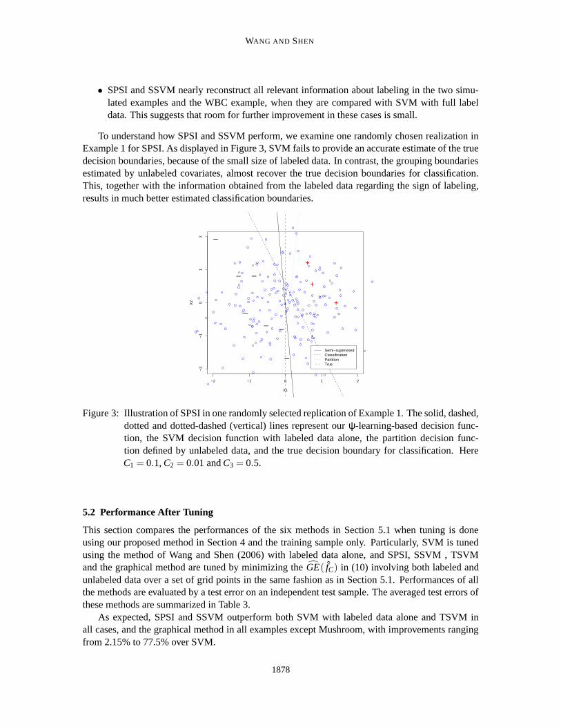
To understand how SPSI and SSVM perform, we examine one randomly chosen realization inExample 1 for SPSI. As displayed in Figure 3, SVM fails to provide an accurate estimate of the truedecision boundaries, because of the small size of labeled data. In contrast, the grouping boundariesestimated by unlabeled covariates, almost recover the true decision boundaries for classification.This, together with the information obtained from the labeled data regarding the sign of labeling,results in much better estimated classification boundaries.

−2 −1 0 1 2

−2

−1

01

2

X1

X2

_

+

+

_

_

_

_+

_

_

Semi−supervisedClassificationPartitionTrue

Figure 3: Illustration of SPSI in one randomly selected replication of Example 1. The solid, dashed,dotted and dotted-dashed (vertical) lines represent our ψ-learning-based decision func-tion, the SVM decision function with labeled data alone, the partition decision func-tion defined by unlabeled data, and the true decision boundary for classification. HereC1 = 0.1, C2 = 0.01 and C3 = 0.5.

5.2 Performance After Tuning

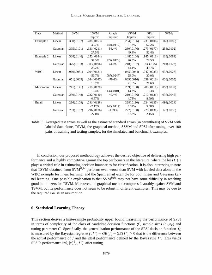
This section compares the performances of the six methods in Section 5.1 when tuning is doneusing our proposed method in Section 4 and the training sample only. Particularly, SVM is tunedusing the method of Wang and Shen (2006) with labeled data alone, and SPSI, SSVM , TSVMand the graphical method are tuned by minimizing the GE( fC) in (10) involving both labeled andunlabeled data over a set of grid points in the same fashion as in Section 5.1. Performances of allthe methods are evaluated by a test error on an independent test sample. The averaged test errors ofthese methods are summarized in Table 3.

As expected, SPSI and SSVM outperform both SVM with labeled data alone and TSVM inall cases, and the graphical method in all examples except Mushroom, with improvements rangingfrom 2.15% to 77.5% over SVM.

1878



Improv. Improve. Improv. Improv.Example 1 Linear .350(.0107) .281(.0153) .234(.0106) .233(.0106) .167(.0085)

36.7% .244(.0112) 61.7% 62.2%Gaussian .395(.0101) .331(.0211) 56.4% .280(.0176) .273(.0177) .258(.0102)

27.5% 49.4% 52.4%Example 2 Linear .338(.0146) .252(.0144) .148(.0104) .145(.0111) .118(.0084)

34.5% .227(.0129) 76.3% 77.5%Gaussian .375(.0153) .303(.0196) 44.6% .248(.0167) .233(.175) .201(.0123)

25.2% 44.4% 49.7%WBC Linear .060(.0081) .094(.0131) .045(.0044) .042(.0035) .037(.0027)

-56.7% .087(.0247) 25.0% 30.0%Gaussian .051(.0039) .044(.0047) -70.6% .039(.0016) .039(.0018) .038(.0005)

13.7% 21.6% 21.6%Mushroom Linear .241(.0141) .211(.0120) .209(.0108) .209(.0111) .053(.0037)

12.4% .137(.0101) 13.3% 13.3%Gaussian .230(.0148) .232(.0140) 40.4% .219(.0156) .210(.0131) .036(.0045)

-0.87% 4.78% 8.69%Email Linear .236(.0109) .241(.0128) .228(.0130) .224(.0125) .099(.0024)

-2.12% .240(.0117) 3.39% 5.08%Gaussian .233(.0107) .296(.0136) -1.69% .227(.0130) .228(.0131) .123(.0056)

-27.0% 2.58% 2.15%

Table 3: Averaged test errors as well as the estimated standard errors (in parenthesis) of SVM withlabeled data alone, TSVM, the graphical method, SSVM and SPSI after tuning, over 100pairs of training and testing samples, for the simulated and benchmark examples.

In conclusion, our proposed methodology achieves the desired objective of delivering high per-formance and is highly competitive against the top performers in the literature, where the loss U(·)plays a critical role in estimating decision boundaries for classification. It is also interesting to notethat TSVM obtained from SVMlight performs even worse than SVM with labeled data alone in theWBC example for linear learning, and the Spam email example for both linear and Gaussian ker-nel learning. One possible explanation is that SVMlight may not have some difficulty in reachinggood minimizers for TSVM. Moreover, the graphical method compares favorably against SVM andTSVM, but its performance does not seem to be robust in different examples. This may be due tothe required Gaussian assumption.

6. Statistical Learning Theory

This section derives a finite-sample probability upper bound measuring the performance of SPSIin terms of complexity of the class of candidate decision functions F , sample sizes (nl,nu) andtuning parameter C. Specifically, the generalization performance of the SPSI decision function fCis measured by the Bayesian regret e( f , f ∗) = GE( f )−GE( f ∗) ≥ 0 that is the difference betweenthe actual performance of f and the ideal performance defined by the Bayes rule f ∗. This yieldsSPSI’s performance infC |e( fC, f ∗)| after tuning.

1879

WANG AND SHEN

6.1 Assumptions and Theorems

Our statistical learning theory involves risk minimization and the empirical process theory. Thereader may consult Shen and Wang (2006) for a discussion about a learning theory of this kind.

First we introduce some notations. Let ( f ∗C,g∗C) = arg inf f ,g∈F ES( f ,g;C) is a minimizer forsurrogate risk ES( f ,g;C), as defined in Lemma 1. Let e f = e( f , f ∗) be the Bayesian regret for fand eg = e(g,g∗C) be the corresponding version for g relative to g∗

C. Denote by V f (X) = L(Y f (X))−L(Y f ∗(X)) and Vg(X) = U(g(X))− U(g∗C(X)) be the differences between f and f ∗, and g and g∗Cwith respect to surrogate loss L and regularized surrogate loss U(g) = U(g)+ C3

2nuC2‖g− f ∗C‖2.

To quantify complexity of F , we define the L2-metric entropy with bracketing. Given any ε > 0,denote {( f l

m, f um)}M

m=1 as an ε-bracketing function set of F if for any f ∈ F , there exists an m suchthat f l

m ≤ f ≤ f um and ‖ f l

m − f um‖2 ≤ ε;m = 1, · · · ,M, where ‖ · ‖2 is the usual L2 norm. Then the

L2-metric entropy with bracketing H(ε,F ) is defined as the logarithm of the cardinality of smallestε-bracketing function set of F .

Three technical assumptions are formulated based upon local smoothness of L, complexity ofF as measured by the metric entropy, and a norm relationship.

Assumption A. (Local smoothness: Mean and variance relationship) For some some constants0 < αh < ∞, 0 ≤ βh < 2, a j > 0; j = 1,2,

sup{h∈F : E(Vh(X))≤δ}

|eh| ≤ a1δαh , (13)

sup{h∈F : E(Vh(X))≤δ}

Var(Vh(X)) ≤ a2δβh , (14)

for any small δ > 0 and h = f ,g.Assumption A describes the local behavior of mean (eh)-and-variance (Var(Vh(X))) relationship.

In (13), Taylor’s expansion usually leads to αh = 1 when f and g can be parameterized. In (14), theworst case is βh = 0 because max(|L(y f )|, |U(g)|) ≤ 2. In practice, values for αh and βh depend onthe distribution of (X ,Y ).

Let J0 = max(J(g∗C),1) with J(g) = 12‖g‖2

− the regularizer. Let Fl(k) = {L(y f )−L(y f ∗) : f ∈F ,J( f )≤ k} and Fu(k) = {U(g)−U(g∗C) : g ∈ F ,J(g)≤ kJ0} be the regularized decision functionspaces for f ’s and g’s.

Assumption B. (Complexity) For some constants ai > 0; i = 3, · · · ,5 and εnv with v = l or u,

supk≥2

φv(εnv ,k) ≤ a5n1/2v , (15)

where φu(ε,k) =R a1/2

3 Tβg/2

u

a4TuH1/2(w,Fu(k))dw/Tu with Tu = Tu(ε,C,k) = min(1,ε2/βg/2+

(nuC2)−1(k/2 − 1)J0), and φl(ε,k) =

R a1/23 T

β f /2

la4Tl

H1/2(w,Fl(k))dw/Tl with Tl = Tl(ε,C,k) =

min(1,ε2/β f /2+(nlC1)−1(k/2−1)max(J( f ∗),1)).

Although Assumption B is always satisfied by some εnv , the smallest possible εnv from (15)yields the best possible error rate, for given Fv and sample size nv. This is to say that the rate isindeed governed by the complexity of Fv(k). An equation of this type, originated from the empiricalprocess theory, has been widely used in quantifying the error rates in function estimation, see, forexample, Shen and Wong (1994).

1880


Assumption C. (Norm relationship) For some constant a6 > 0, ‖ f‖1 ≤ a6‖ f‖ for any f ∈ F ,where ‖ · ‖1 is the usual L1-norm.

Assumption C specifies a norm relationship between norm ‖ · ‖ defined by a RKHS and ‖ · ‖1.This is usually met when F is a RKHS, defined, for instance, by Gaussian and Sigmoid kernels,compare with Adams (1975).

Theorem 3 (Finite-sample probability bound for SPSI) In addition to Assumptions A-C, assumethat nl ≤ nu. For the SPSI classifier Sign( fC), there exist constants a j > 0; j = 1,6,7,10,11, andJl > 0, Ju > 0 and B ≥ 1 defined as in Lemma 5, such that

P(

infC

|e( fC, f ∗)| ≥ a1sn)≤ 3.5exp(−a7nu((nuC∗

2)−1J0)

max(1,2−βg))+

6.5exp(−a10nl((nlC∗1)

−1 min(Jl,J( f ∗)))max(1,2−β f ))+

6.5exp(−a11nu((nuC∗2)

−1Ju)max(1,2−βg)),

where sn = min(δ2α f

nl ,max(δ2αgnu , infC∈C |e(g∗C, f ∗)|)

), δnv = min(εnv ,1) with v = l,u, C∗ =

(C∗1 ,C

∗2 ,C

∗3) = arg infC∈C |e(g∗C, f ∗)|), and C = {C : nlC1 ≥ 2δ−2

nlmax(Jl,J( f ∗),1),nuC2 ≥

2δ−2nu

max(J0,2C3(2B+ J( f ∗C)+ J(g∗C))),C3 ≥ a26Bδ−4

nu}.

Corollary 4 Under the assumptions of Theorem 3, as nu ≥ nl → ∞,

infC

|e( fC, f ∗)| = Op(sn), sn = min(δ2α f

nl ,max(δ2αgnu , inf

C∈C|e(g∗C, f ∗)|)

).

Theorem 3 provides a probability bound for the upper tail of |e( fC, f ∗)| for any finite (nl,nu).Furthermore, Corollary 4 says that the Bayesian regret infC∈C |e(g∗C, f ∗)| for the SPSI classifierSign( fC) after tuning is of order of no larger than sn, when nu ≥ nl → ∞. Asymptotically, SPSI per-

forms no worse than its supervised counterpart in that infC |e( fC, f ∗)| = Op(δ2α fnl ). Moreover, SPSI

can outperform its supervised counterpart in the sense that infC |e( fC, f ∗)| = Op(min(δ2αgnu ,δ2α f

nl )) =

Op(δ2αgnu ), when {g∗C : C ∈ C} provides a good approximation to the Bayes rule f ∗.

Remark: Theorem 3 and Corollary 4 continue to hold when the “global” entropy in (15) isreplaced by a “local” entropy, compare with Van De Geer (1993). Let Fl,ξ(k) = {L(y f )−L(y f ∗) :f ∈ F ,J( f ) ≤ k, |e( f , f ∗)| ≤ ξ} and Fu,ξ(k) = {U(g)−U(g∗C) : g ∈ F ,J(g) ≤ k, |e(g,g∗C)| ≤ ξ}be the “local” entropy of Fl(k) and Fu(k). The proof requires only a slight modification. The localentropy avoids a loss of lognu factor in the linear case, although it may not be useful in the nonlinearcase.

6.2 Theoretical Examples

We now apply the learning theory to one linear and one kernel learning examples to obtain thegeneralization error rates for SPSI, as measured by the Bayesian regret. We will demonstrate thatthe error in the linear case can be arbitrarily fast while that in the nonlinear case is fast. In eithercase, SPSI’s performance is better than that of its supervised counterpart.

Linear learning: Consider linear classification where X = (X(1),X(2)) is sampled independentlyaccording to the same probability density q(z) = 1

2(θ + 1)|z|θ for z ∈ [−1,1] with θ ≥ 1. Given X ,assign label Y to 1 if X(1) > 0 and −1 otherwise; then Y is chosen randomly to flip with constant

1881

WANG AND SHEN

probability τ for 0 < τ < 12 . Here the true decision function ft(x) = x(1) yielding the vertical line as

the classification boundary.In this case, the degree of smoothness of this problem is characterized by exponent θ > 0 in the

density q(z), which describes the level of difficulty of linear classification but may not be so in thenonlinear case.

For classification, we minimize (2) over F , consisting of linear decision functions of formf (x) = (1,x)T w for w ∈ R 3 and x = (x(1),x(2)) ∈ R 2. To apply Corollary 4, we verify Assump-tions A-C with detailed verification given in Appendix B. In fact, Assumption A follows from thesmoothness of E(Vh(X)) and Var(Vh(X)) with respect to h, where a local Taylor expansion yieldsthe degree of smoothness exponents α and β. Assumption B is automatically met, and the entropyEquation (15) is solved for the smallest possible εnv satisfying it. Assumption C is always true

for RKHS. It then follows from Corollary 4 that infC |e( fC, f ∗)| = Op(n−(θ+1)/2u (lognu)

(θ+1)/2) asnu ≥ nl → ∞. This says that the optimal ideal performance of the Bayes rule is recovered by SPSIat speed of n−(θ+1)/2

u (lognu)(θ+1)/2 as nu ≥ nl → ∞. This rate is arbitrarily fast as θ → ∞.

Kernel learning: Consider, in the preceding case, kernel learning with a different candidatedecision function class defined by the Gaussian kernel. To specify F , we may embed a finite-dimensional Gaussian kernel representation into an infinite-dimensional space F = {x∈R 2 : f (x) =wT

f φ(x) = ∑∞k=0 w f ,kφk(x) : w f = (w f ,0, · · ·)T ∈ R ∞} by the representation theorem of RKHS, com-

pare with Wahba (1990). Here 〈φ(x),φ(z)〉 = K(x,z) = exp(− ‖x−z‖2

2σ2 ).To apply Corollary 4, we verify Assumptions A-C as before, with detailed verification given

in Appendix B. The function space F generated by the Gaussian kernel is rich enough to wellapproximate the ideal performer Sign(E(Y |X)) (Steinwart, 2001), and yields the exponents α andβ in Assumption A with smoothness and Soblev’s inequality (Adams, 1975). Similarly, it followsfrom Corollary 4 that infC |e( fC, f ∗)|= Op(min(n−1

l (lognlJl)3,n−1/2

u (lognuJu)3/2)) as nu ≥ nl → ∞.

Therefore, the optimal ideal performance of the Bayes rule is recovered by SPSI at fast speed ofmin(n−1

l (lognlJl)3,n−1/2

u (lognuJu)3/2) as nu ≥ nl → ∞.

7. Discussion

This article proposed a novel large margin semi-supervised learning methodology that is applicableto a class of large margin classifiers. In contrast to most semi-supervised learning methods assumingvarious dependencies between the marginal and conditional distributions, the proposed methodol-ogy integrates labeled and unlabeled data through regularization to identify such dependencies forenhancing classification. The theoretical and numerical results show that our methodology outper-forms SVM and TSVM in situations when unlabeled data provides useful information, and performsno worse when unlabeled data does not so. For tuning, further investigation of regularization pathsof our proposed methodology is useful as in Hastie, Rosset, Tibshirani and Zhu (2004), to reducecomputational cost.

Acknowledgments

This research is supported by NSF grants IIS-0328802 and DMS-0604394. We thank Wei Pan formany constructive comments. We also thank three referees and the editor for helpful comments andsuggestions.

1882


Appendix A. Technical Proofs

Proof of Theorem 2: The proof is similar to that of Theorem 2 of Wang and Shen (2006), and thusis omitted.Proof of Theorem 3: The proof uses a large deviation empirical technique for risk minimization.Such a technique has been previously developed in function estimation as in Shen and Wong (1994).The proof proceeds in three steps. In Step 1, the tail probability of {eU(gC,g∗C) ≥ δ2

nu} is bounded

through a large deviation probability inequality of Shen and Wong (1994). In Step 2, a tail prob-ability bound of {|e( fC, f ∗)| ≥ δ2

nu} is induced from Step 1 using a conversion formula between

eU(gC,g∗C) and |e( fC, f ∗)|. In Step 3, a probability upper bound for {|e( fC, f ∗)| ≥ δ2nl} is obtained

using the same treatment as above. The desired bound is obtained based on the bounds in Step 2and Step 3.

Step 1: It follows from Lemma 5 that max(‖ fC‖2,‖gC‖2) ≤ B for a constant B ≥ 1, where( fC, gC) is the minimizer of (2). Furthermore, gC defined in (2) can be written as gC =argmin

g∈F

{C2 ∑n

j=nl+1U(g(x j))+ J(g)+ C32 (‖ fC −g‖2 −‖ f ∗C −g‖2)

}.

By the definition of gC, P(eU(gC,g∗C) ≥ δ2nu

) is upper bounded by

P(J(gC) ≥ B)+P∗(

supg∈N

n−1u

n

∑j=nl+1

(U(g∗C(x j))−U(g(x j)))+λ(J(g∗C)− J(g))

+λC3

2(‖ fC −g∗C‖2 −‖ f ∗C −g∗C‖2 −‖ fC −g‖2 +‖ f ∗C −g‖2) ≥ 0

)

≤ P(J(gC) ≥ B)+P∗(

supg∈N

n−1u

n

∑j=nl+1

(U(g∗C(x j))−U(g(x j)))+λ(J(g∗C)− J(g))

+λC3(2B+ J( f ∗C)+ J(g∗C)) ≥ 0)≡ P(J(gC) ≥ B)+ I,

where λ = (nuC2)−1, N = {g ∈ F ,J(g) ≤ B,eU(g,g∗C) ≥ δ2

nu}, and P∗ denotes the outer probability.

By Lemma , there exists constants a10,a11 > 0 such that P(J(gC)≥ B)≤ 6.5exp(−a10nl(nlC1)−1Jl)

+6.5exp(−a11nu(nuC2)−1Ju), where Jl and Ju are defined in Lemma 5.

To bound I, we introduce some notations. Define the scaled empirical process as Eu(U(g∗C)−U(g)) = n−1

u ∑nj=nl+1

(U(g∗C(x j)) − U(g(x j)) + λ(J(g∗C) − J(g))

)− E(U(g∗C(X j)) − U(g(X j))+

λ(J(g∗C)− J(g))) = Eu(U(g∗C)−U(g)). Thus

I = P∗(

supg∈N

Eu(U(g∗C)−U(g)) ≥

infg∈N

E(U(g(X))−U(g∗C(X)))+λ(J(g∗C)− J(g))−λC3(2B+ J( f ∗C)+ J(g∗C))

).

Let As,t = {g ∈ F : 2s−1δ2nu≤ eU(g,g∗C) < 2sδ2

nu,2t−1J0 ≤ J(g) < 2tJ0}, and let As,0 = {g ∈ F :

2s−1δ2nu≤ eU(g,g∗C) < 2sδ2

nu,J(g) < J0}; s, t = 1,2, · · · . Without loss of generality, we assume that

εnu < 1. Then it suffices to bound the corresponding probability over As,t ; s, t = 1,2, · · · . Towardthis end, we control the first and second moment of U(g∗C(X))−U(g(X)) over f ∈ As,t .

For the first moment, by assumption δ2nu≥ 2λmax(J0,2C3(2B+ J( f ∗C)+ J(g∗C))),

infAs,t

E(U(g(X))−U(g∗C(X)))+λ(J(g∗C)− J(g)) ≥ 2s−1δ2nu

+λ(2t−1 −1)J0;s, t = 1,2, · · · ,

1883

WANG AND SHEN

infAs,0

E(U(g(X))−U(g∗C(X)))+λ(J(g∗C)− J(g)) ≥ (2s−1 −1/2)δ2nu≥ 2s−2δ2

nu;s = 1,2, · · · .

Therefore, infAs,t E(U(g(X))−U(g∗C(X)))+λ(J(g∗C)−J(g))−λC3(2B+J( f ∗C)+J(g∗C))≥M(s, t) =

2s−2δ2nu

+λ(2t−1−1)J0, and infAs,0 E(U(g(X))−U(g∗C(X)))+λ(J(g∗C)−J(g))−λC3(2B+J( f ∗C)+J(g∗C)) ≥ M(s,0) = 2s−3δ2

nu, for all s, t = 1,2, · · · .

For the second moment, by Assumptions A,

supAs,t

Var(U(g(X))−U(g∗C(X))) ≤ supAs,t

a2(eU(g,g∗C))βg ≤ a2(2sδ2

nu+(2t −1)λJ0)

βg

≤ a223βg(2s−2δ2nu

+(2t−1 −1)λJ0)βg ≤ a3M(s, t)βg = v2(s, t),

for and s, t = 1,2, · · · and some constant a3 > 0.Now I ≤ I1 + I2 with I1 = ∑∞

s,t=1 P∗(supAs,t

Eu(U(g∗C)

−U(g)) ≥ M(s, t)); I2 = ∑∞s=1 P∗(sup

As,0

Eu(U(g∗C)−U(g)) ≥ M(s,0)). Next we bound I1 and I2

separately using Theorem 3 of Shen and Wong (1994). We now verify conditions (4.5)-(4.7)there. To compute the metric entropy of {U(g)−U(g∗

C) : g ∈ As,t} in (4.7) there, we note thatR v(s,t)

aM(s,t) H1/2(w,Fu(2t))dw/M(s, t) is nonincreasing in s and M(s, t) and hence that

Z v(s,t)

aM(s,t)H1/2(w,Fu(2

t))dw/M(s, t) ≤Z a1/2

3 M(1,t)βg/2

aM(1,t)H1/2(w,Fu(2

t))dw/M(1, t)

≤ φ(εnu ,2t),

with a = 2a4ε. Assumption B implies (4.7) there with ε = 1/2 and some ai > 0; i = 3,4. Further-more, M(s, t)/v2(s, t) ≤ 1/8 and T = 1 imply (4.6), and (4.7) implies (4.5). By Theorem 3 of Shenand Wong (1994), for some constant 0 < ζ < 1,

I1 ≤∞

∑s,t=1

3exp

(− (1−ζ)nuM2(s, t)

2(4v2(s, t)+M(s, t)/3)

)≤

∞

∑s,t=1

3exp(−a7nu(M(s, t))max(1,2−βg))

≤∞

∑s,t=1

3exp(−a7nu(2s−1δ2

nu+λ(2t−1 −1)J0)

max(1,2−βg))

≤ 3exp(−a7nu(λJ0)max(1,2−βg))/(1− exp(−a7nu(λJ0)

max(1,2−βg)))2.

Similarly, I2 ≤ 3exp(−a7nu(λJ0)max(1,2−βg))/(1−exp(−a7nu(λJ0)

max(1,2−βg)))2. Thus I ≤ I1 + I2 ≤6exp(−a7nu((nuC2)

−1J0)max(1,2−βg))/(1−exp(−a7nu((nuC2)

−1J0)max(1,2−βg)))2, and I1/2 ≤ (2.5+

I1/2) exp(−a7nu((nuC2)−1J0)

max(1,2−βg)). Thus P(eU(gC,g∗C) ≥ δ2nu

) ≤ 3.5exp(−a7nu

((nuC2)−1J0)

max(1,2−βg)) + 6.5exp(−a10nl((nlC1)−1Jl)

max(1,2−β f ))+6.5exp(− a11nu((nuC2)

−1Ju)max(1,2−β f )).

Step 2: By Lemma 5 and Assumption C, |eU( fC, gC)| ≤ E| fC(X)− gC(X)| ≤ a6‖ fC − gC‖ ≤a6√

B/C3 ≤ δ2nu

when C3 ≥ a26Bδ−4

nu. By Assumption A and the triangle inequality, |e( fC,g∗C)| ≤

a1(eU( fC,g∗C))αg ≤ a1(eU(gC,g∗C) + |eU( fC, gC)|)αg ≤ a1(eU(gC,g∗C) + δ2nu

, implying thatP(|e( fC,g∗C)| ≥ a1(2δ2

nu)αg)≤P(eU(gC,g∗C)≥ δ2

nu), ∀C ∈ C . Then P

(infC |e( fC, f ∗)| ≥ a1(2δ2

nu)αg +

infC∈C |e(g∗C, f ∗)|)

≤ P(eU(gC∗ ,g∗C∗) ≥ δ2nu

) ≤ 3.5exp(− a7nu((nuC∗2)

−1J0)max(1,2−βg)) +

1884


6.5exp(−a10nl((nlC∗1)

−1Jl)max(1,2−β f )) + 6.5exp(−a11nu ((nuC∗

2)−1Ju)

max(1,2−βg)), where C∗ =arg infC∈C |e(g∗C, f ∗)|.

Step 3: Note that fC = argmax f∈F {C1 ∑nli=1 L(yi f (xi)) + 1

2‖ f‖2−} when C2 = 0 and C3 = ∞.

An application of the same treatment yields that P(infC e( fC, f ∗) ≥ a1δ2nl) ≤ P(infC eL( fC, f ∗) ≥

a1δ2nl) ≤ 3.5exp(−a10nl((nlC∗

1)−1J( f ∗))max(1,2−β f )) when nlC∗

1 ≥ 2δ−2nl

max(J( f ∗),1). The desiredresult follows.

Lemma 5 Under the assumptions of Theorem 3, for ( fC, gC) as the minimizer of (2), there existsconstants B > 0, depending only on C1, such that

max(E(C3‖ fC − gC‖2 +‖gC‖2),E‖ fC‖2,2C1) ≤ B.

Proof: It suffices to show E(C3‖ fC− gC‖2+‖gC‖2)≤B. Let W ( f ,g) = 1C1

s( f ,g) = ∑nli=1Wl(yi f (xi))

+C2C1

∑nj=nl+1Wu(g(x j)), where Wl( f (xi)) = L(yi f (xi))+

C34nlC1

‖ f −g‖2, and Wu(g(x j)) =U(g(x j))+1

2nuC2‖g‖2 + C3

4nuC2‖ f −g‖2. For convenience, write Jl( f ,g) = C3

4 ‖ f −g‖2, Ju( f ,g) = C34 ‖ f −g‖2 +

12‖g‖2

−, λl = (C1nl)−1, and λu = (C2nu)

−1. We then define a new empirical process El,u(W ( f ,g)−W ( f ∗C,g∗C)) = El(Wl( f )−Wl( f ∗C))+ C2nu

C1nlEu(Wu(g)−Wu(g∗C)) as

1nl

nl

∑i=1

(Wl( f (xi))−Wl( f ∗C(xi))−E(Wl( f (Xi))−Wl( f ∗C(Xi)))

)+

C2nu

C1nl

1nu

n

∑i=nl+1

(Wu(g(x j))−Wu(g

∗C(xi))−E(Wu(g(X j))−Wu(g

∗C(Xi)))

).

An application of the same argument as in the proof of Theorem 3 yields that for constants a8,a9 > 0,P(eW ( fC, gC; f ∗C,g∗C) ≥ δ2

w) is upper bounded by

3.5exp(−a8nl((nlC1)−1Jl)

max(1,2−β f ))+3.5exp(−a9nu((nuC2)−1Ju)

max(1,2−βg)),

provided that 2Jl ≤ nlC1δ2nl

and 2Ju ≤ nuC2δ2nu

, where eW ( f ,g; f ∗C,g∗C) = eL( f , f ∗C) + C2C1

eU(g,g∗C),

δ2w = δ2

nl+ C2nu

C1nlδ2

nu, Jl = max(Jl( f ∗C,g∗C),1) and Ju = max(Ju( f ∗C,g∗C),1).

Without loss of generality, assume min(Jl( f ∗C,g∗C),Ju( f ∗C,g∗C)) ≥ 1. Let J( f ,g) = Jl( f ,g) +Ju( f ,g) and At = { f ,g∈F : eW ( f ,g; f ∗C,g∗C)≤ δ2

w,2t−1J( f ∗C,g∗C)≤ J( f ,g) < 2tJ( f ∗C,g∗C)}; t = 1, · · · .Then, P

(J( fC, gC) ≥ J( f ∗C,g∗C)

)is upper bounded by

P(eW ( fC, gC; f ∗C,g∗C) ≥ δ2w)+

∞

∑t=1

P∗(

supAt

El,u(W ( f ∗C,g∗C)−W ( f ,g)) ≥ E(W ( f ,g)−W ( f ∗C,g∗C))

)

≤ P(eW ( fC, gC; f ∗C,g∗C) ≥ δ2w)+

∞

∑t=1

P∗(

supAt

El,u(W ( f ∗C,g∗C)−W ( f ,g)) ≥ (2t−1 −1)λlJ( f ∗C,g∗C)+ δ2w

)

≤ P(eW ( fC, gC; f ∗C,g∗C) ≥ δ2w)+

∞

∑t=1

P∗(

supAt

El(Wl( f ∗C)−Wl( f )) ≥ (2t−1 −1)λlJl + δ2nl

)+

∞

∑t=1

P∗(

supAt

Eu(Wu(g∗C)−Wu(g)) ≥ (2t−1 −1)λuJu + δ2

nu

).

1885

WANG AND SHEN

An application of the same argument in the proof of Theorem 3 yields that for some constants0 < a10 ≤ a8 and 0 < a11 ≤ a9 that P

(J( fC, gC) ≥ J( f ∗C,g∗C)

)is upper bounded by

P(eW ( f ,g; f ∗C,g∗C) ≥ δ2w)+

∞

∑t=1

(3exp(−a11nl((nlC1)

−1Jl( f ∗C,g∗C)2t−1)max(1,2−β f ))+

3exp(−a12nu((nuC2)−1Ju( f ∗C,g∗C)2t−1)max(1,2−βg))

)

≤ 6.5exp(−a10nl((nlC1)−1Jl)

max(1,2−β f ))+6.5exp(−a11nu((nuC2)−1Ju)

max(1,2−βg)).

Note that J( fC, gC) ≤ s( f , g) ≤ s(1,1) ≤ 2C1nl . There exists a constant B1 > 0 such that

E(C3‖ fC − gC‖2 +‖gC‖2−) ≤ J( f ∗C,g∗C)+B1 ≤ 2C1 +B1, (16)

since J( f ∗C,g∗C) ≤ ES( f ∗C,g∗C) ≤ ES(1,1) ≤ 2C1. It follows from the KKT condition and (16) thatE|wgC,0| is bounded by a constant B2, depending only on C1. The desired result follows with achoice of B = 2C1 +B1 +B2

2.

Lemma 6 (Metric entropy in Example 6.2.1) Under the assumptions there, for v = l or u,

H(ε,Fv,ξ(k)) ≤ O(log(ξ1/(θ+1)/ε)).

Proof: We first show the inequality for Fu,ξ(k). Suppose lines g(x) = 0 and g∗C(x) = 0 inter-sect lines x(2) = ±1 with two points (ug,1),(vg,−1) and (ug∗C ,1),(vg∗C ,−1), respectively. Note

that e(g,g∗C) ≤ ξ implies P(∆(g,g∗C)) ≤ ξ1−2τ with ∆(g,g∗C) = {Sign(g(x)) 6= Sign(g∗C(x))}. Direct

calculation yields that P(∆(g,g∗C)) ≥ 12 max(|ug − ug∗C |, |vg − vg∗C |)

θ+1, max(|ug − ug∗C |, |vg − vg∗C |) ≤a′ξ1/(θ+1) for a constant a

′> 0. We then cover all possible (ug,1) and (vg,−1) with intervals

of length ε∗. The covering number for these possible points is no more than (2a′ξ1/(θ+1)/ε∗)2.After these points are covered, we then connect the endpoints of the covering intervals to formbracket planes l(x) = 0 and u(x) = 0 such that l ≤ g ≤ u, and ‖u − l‖2 ≤ ‖u − l‖∞ ≤ ε∗. LetU l(g) = 2− 2max(|l±1|, |u±1|) and Uu(g) = 2− 2I(l(x)u(x) > 0)min(|l±1|, |u±1|), then U l(g) ≤U(g)≤Uu(g) and ‖Uu(g)−U l(g)‖∞ ≤ 2‖|u− l‖∞ ≤ 2ε∗. With ε = 2ε∗, {(U l(g),Uu(g))} forms anε-bracketing set of U(g). Therefore, the ε-covering number for Fu,ξ(k) is at most (4a′ξ1/(θ+1)/ε)2,

implying H(ε,Fu,ξ(k)) is upper bounded by O(log(ξ1

θ+1 /ε)). Furthermore, it is similar to showthe inequality for Fl,ξ(k) since

(2min(1,1−max(yl(x),yu(x))+),2min(1,1−min(yl(x),yu(x))+)

)

forms a bracket for L(y f (x)) when l ≤ f ≤ u.

Lemma 7 (Metric entropy in Example 6.2.2) Under the assumptions there, for v = l or u,

H(ε,Fv(k)) ≤ O((log(k/ε))3).

Proof: We first show the inequality for Fu(k). Suppose there exist ε-brackets (glm,gu

m)Mm=1 for some

M such that for any g ∈ F (k) = {g ∈ F : J(g)≤ k}, glm ≤ g ≤ gu

m and ‖gum−gl

m‖∞ ≤ ε for some 1 ≤m≤M. Let U l(g) = 2−2max(|gl

m,±1|, |gum,±1|) and Uu(g) = 2−2I(gl

mgum > 0)min(|gl

m,±1|, |gum,±1|),

then U l(g) ≤ U(g) ≤ Uu(g) and ‖Uu(g)−U l(g)‖∞ ≤ 2‖gum − gl

m‖∞ ≤ 2ε. Therefore, (U l(g)−U(g∗C),Uu(g)−U(g∗C)) forms a bracket of length 2ε for U(g)−U(g∗

C). The desired inequality thenfollows from the Example 4 in Zhou (2002) that H∞(ε,F (k))≤ O(log(k/ε)3) under the L∞−metric:‖g‖∞ = supx∈R 2 |g(x)|. Furthermore, it is similar to show the inequality for Fl(k) as in Lemma 6.

1886


Lemma 8 For any functions f , g and any constant ρ > 0,

E|Sign( f (X))−Sign(g(X))|I(| f (X)| ≥ ρ) ≤ 2ρ−1E| f (X)−g(X)|.

Proof: The left hand side is 2P(| f (X)| ≥ ρ,Sign( f (X)) 6= Sign(g(X))) ≤ 2P(| f (x)−g(x)| ≥ ρ) ≤2ρ−1E| f (X)−g(X)| by Chebyshev’s inequality.

Appendix B. Verification of Assumptions A-C in the Theoretical Examples

Linear learning: Since (X(1),Y ) is independent of X(2), ES( f ,g;C) = E(E(S( f ,g;C)|X(2))) ≥ES( f ∗C, g∗C;C) for any f ,g ∈ F , and ( f ∗C, g∗C) = argmin f ,g∈F1

ES( f , g;C) with F1 = {x(1) ∈ R :f (x) = (1,x(1))

T w : w ∈ R 2} ⊂ F . It then suffices to verify Assumptions A-C over F1 ratherthan F . By Lemma 1, the approximation error infC∈C e(g∗C, f ∗) = 0. For (13), note that f ∗ mini-mizes EL(Y f (X)) and g∗C minimizes EU(g) given f ∗C . Direct computation, together with Taylor’sexpansion yields that E(Vh(X)) = (e0,e1)Γh(e0,e1)

T for any function h = (1,x(1))T wh ∈ F1 with

wh = wh∗ +(e0,e1)T , where h∗ = f ∗ or g∗C and Γh is a positive definite matrix. Thus E(Vh(X)) ≥

λ1(e20 + e2

1) for constant λ1 > 0. Moreover, straightforward calculation yields that |eh| ≤ 12(1−

2τ)min(|wh∗,1|, |wh∗,1 + e1|)−(θ+1)|e0|θ+1 ≤ λ2(e20 + e2

1)(θ+1)/2 for some constant λ2 > 0, where

wh∗ = (wh∗,0,wh∗,1). A combination of these two inequalities leads to (13) with αh = (θ + 1)/2.For (14), note that Var(Vh(X)) ≤ ‖h− h∗‖2

2 = e20 + e2

1EX2(1) ≤ max(1,EX2

(1))(e20 + e2

1). This implies

(14) with βh = 1. For Assumption B, by Lemma 6, H(ε,Fv,ε(k)) ≤ O(log(ε1/(θ+1))/ε) for any

given k, thus φv(ε,k) = a3(log(T−θ/2(θ+1)v ))1/2/T 1/2

v with Tv = Tv(ε,C,k). Hence supk≥2 φv(ε,k) ≤O((log(ε−θ/(θ+1)))1/2/ε

)in (15). Solving (15), we obtain εnl = ( lognl

nl)1/2 when C1 ∼

J( f ∗)δ−2nl

n−1l ∼ lognl and εnu = ( lognu

nu)1/2 when C2 ∼ J0δ−2

nun−1

u ∼ lognu. Assumption C is fulfilled

because E(X2) < ∞. In conclusion, we obtain, by Corollary 4, that infC |e( fC, f ∗)| =Op((n−1

u lognu)(θ+1)/2). Surprisingly, this rate is arbitrarily fast as θ → ∞.

Kernel learning: Similarly, we restrict our attention to F1 = {x ∈ R : f (x) = wTf φ(x) =

∑∞k=0 w f ,kφk(x) : w f ∈ R ∞}, where 〈φ(x), φ(z)〉 = exp(− (x−z)2

2σ2 ).For (13), note that F is rich for sufficiently large nl in that for any continuous function f , there

exists a f ∈ F such that ‖ f − f‖∞ ≤ ε2nl

, compare with Steinwart (2001). Then f ∗ = argmin f∈FEL(Y f ) implies ‖ f ∗ − Sign(E(Y |X))‖∞ ≤ ε2

nland |EL(Y f ∗)− GE( f ∗)| ≤ 2ε2

nl. Consequently,

|e( f , f ∗)| ≤ E(V f (X)) + 2ε2nl

and α f = 1. On the other hand, E(Vg(X)) ≥ −E|g− f ∗C| −E|g∗C −f ∗C|+ C3

2nuC2‖g− f ∗C‖2 − C3

2 ‖g∗C − f ∗C‖2. Using the fact that ( f ∗C,g∗C) is the minimizer of ES( f ,g;C),

we have C32 ‖g∗C − f ∗C‖2 ≤ ES( f ∗C,g∗C) ≤ ES(1,1) ≤ 2C1. By Sobolev’s inequality (Adams, 1975),

E|g∗C − f ∗C| ≤ λ3‖g∗C − f ∗C‖ ≤ λ3(4C1/C3)1/2 and E|g− f ∗C| ≤ λ3‖g− f ∗C‖, for some constant λ3 > 0.

Plugging these into the previous inequality, we have eU(g,g∗C) ≥ C32nuC2

‖g− f ∗C‖2 − λ3‖g− f ∗C‖−2C1nuC2

− λ3(4C1/C3)1/2. By choosing suitable C, we obtain 1

2‖g− f ∗C‖2 − eU(g,g∗C)1/2‖g− f ∗C‖−eU(g,g∗C) ≤ 0. Solving this inequality yields ‖g− f ∗C‖ ≤ (1 +

√5)eU(g,g∗C)1/2. Furthermore, by

Lemma 8 and Sobolev’s inequality, for sufficient small λ4 > 0, e(g,g∗C) ≤ E2λ−14 | f ∗C(X)−g(X)|+

2P(| f ∗C(X)| ≤ λ4)+ e( f ∗C,g∗C) ≤ 2λ−14 (1 +

√5)E(Vg(X))1/2 + 2P(| f ∗C(X)| ≤ λ4)+ e( f ∗C,g∗C). How-

ever, by Lemma 1, e( f ∗C,g∗C) → 0, and P(| f ∗C(X)| ≤ λ4) ≤ P(| f ∗(X)| − | f ∗(X)− f ∗C(X)| ≤ λ4) =P(| f ∗(X)| ≤ | f ∗(X)− f ∗C(X)|+ λ4) → 0, as C1,C2,C3 → ∞, because of linearity of f ∗. This yields(13) with αg = 1/2. For (14), Var(L(Y f (X))− L(Y f ∗(X))) ≤ 2E(L(Y f (X))− L(Y f ∗(X)))2 =

1887

WANG AND SHEN

(w f − w f ∗)T Γ2(w f − w f ∗) where Γ2 is a positive definite matrix, and similar to Example 6.2.1,

E(Vf (X)) = (w f −w f ∗)Γh(w f −w f ∗)T since f ∗ minimizes E(L(Y f (X))). Therefore, there exists

a constant λ5 > 0 such that Var(L(Y f (X))− L(Y f ∗(X))) ≤ λ5E(Vf (X)). Also, Var(U(g(X))−U(g∗C(X))) ≤ ‖g−g∗C‖2

2 ≤ 2(‖g− f ∗C‖2 +‖g∗C − f ∗C‖2) ≤ 2((1+√

3)2eU(g,g∗C)+ 4C1C3

) ≤ (8+2(1+√3)2)E(Vg(X))), implying (14) with β f = βg = 1. For Assumption B, by Lemma 7, H(ε,Fv(k)) ≤

O((log(kJv/ε))3) for any given k. Similarly, we have εnl = (n−1l (lognlJl)

3)1/2 when C1 ∼J( f ∗)δ−2

nln−1

l ∼ (lognlJl)−3 and εnu = (n−1

u (lognuJu)3)1/2 when C2 ∼ J0δ−2

nun−1

u ∼ (lognuJu)−3. As-

sumption C is fulfilled with the Gaussian kernel.

Appendix C. The Dual Form of (5)

Let ∇ψ(k) = (∇ψ(k)1 ,∇ψ(k)

2 )T , ∇ψ(k)1 = C1(∇ψ2(y1 f (k)(x1))y1, · · · ,∇ψ2(ynl f (k)(xnl ))ynl ) and ∇ψ(k)

2 =2C2(∇U2(g(k)(xnl+1)), · · · ,∇U2(g(k)(xn))). Further, let α = (α1, · · · ,αnl )

T , β = (βnl+1, · · · ,βn)T ,

γ = (γnl+1, · · · ,γn)T , yα = (y1α1, · · · ,ynl αnl )

T , and

Theorem 9 (ψ-learning) The dual problem of (4) with respect to (α,β,γ) is

maxα,β,γ

{−(

yαβ− γ

)T ((1+ 1

C3)Kll +

1C3

Il Klu

Kul Kuu

)(yα

β− γ

)+

(α− (β+ γ))T 1n − (yα − (β− γ))T

(K∇ψ(k) +

(∇ψ(k)

10nu

))},

(17)

subject to

(2

(yα

γ−β

)+∇ψ(k)

)T

1n = 0, 0n ≤ α ≤C11n, 0n ≤ β, 0n ≤ γ, and 0n ≤ β+ γ ≤C21n.

Proof of Theorem 9: For simplicity, we only prove the linear case as the nonlinear case is es-sentially the same. The kth primal problem in (4), after introducing slack variable ξ, is equivalentto min(w f ,wg,ξi,ξ j)C1 ∑nl

i=1 ξi +C2 ∑nj=nl+1 ξ j +

C32 ‖w f −wg‖2 + 1

2‖wg‖2 −〈w,∇sψ2 ( f (k),g(k))〉 subject

to constraints 2(1 − yi(〈w f ,xi〉)) ≤ ξi, xi ≥ 0; i = 1, · · · ,nl , and 2(|〈wg,x j〉| − 1) ≤ ξ j, ξ j ≥ 0;j = nl +1, · · · ,n.

To solve this minimization problem, the Lagrangian multipliers are employed to yield

L(w f ,wg,ξi,ξ j)

= C1

nl

∑i=1

ξi +C2

n

∑j=nl+1

ξ j +C3

2‖w f −wg‖2 +

12‖wg‖2 −〈w,∇sψ

2 (w(k)f ,w(k)

g )〉+

2nl

∑i=1

αi(1− yi(〈w f ,xi〉)−ξi

2)+2

n

∑j=nl+1

β j(〈wg,x j〉−1− ξ j

2)−

2n

∑j=nl+1

γ j(〈wg,x j〉+1+ξ j

2)−

nl

∑i=1

γiξi −n

∑j=nl+1

η jξ j, (18)

where αi ≥ 0; i = 1, · · · ,nl , β j ≥ 0, γ j ≥ 0, j = nl + 1, · · · ,n. Differentiate L with respect to(w f ,wg,ξi,ξ j) and let the partial derivatives be zero, we obtain that ∂L

∂w f=C3(w f −wg)−2∑nl

i=1 αiyixi

−∇ψ(k)1 f = 0, ∂L

∂wg= wg −C3(w f − wg)−2∑n

j=nl+1(γ j −β j)x j −∇ψ(k)1g = 0, ∂L

∂w f ,0= C3(w f ,0 −wg,0)−

1888


2∑nli=1 αiyi = 0, ∂L

∂wg,0= −C3(w f ,0 −wg,0)− 2∑n

j=nl+1(γ j −β j)−∇ψ(k)2g = 0, ∂L

∂ξi= C1 −αi − γi = 0,

and ∂L∂ξ j

= C2 −β j − γ j −η j = 0. Solving these equations yields that w∗f = 2(1+C−1

3 )∑nli=1 αiyixi +

∑nj=nl+1(γ j − β j)x j + (1 + C−1

3 )∇ψ(k)1 f + ∇ψ(k)

1g , w∗g = 2∑nl

i=1 αiyixi + ∑nj=nl+1(γ j − β j)x j + ∇ψ(k)

1 f +

∇ψ(k)1g , 2∑nl

i=1 αiyi + 2∑nj=nl+1(γ j − β j) + ∇ψ(k)

2 f + ∇ψ(k)2g = 0, αi + γi = C1; i = 1, · · · ,nl , and β j +

γ j + η j = 0; j = nl + 1, · · · ,n. Substituting w∗f , w∗

g and these identities into (18), we obtain (17)after ignoring all constant terms. To derive the corresponding constraints, note that C1−αi−γi = 0,γi ≥ 0 and αi ≥ 0 implies 0 ≤ αi ≤ C1, η j ≥ 0 and C2 − β j − γ j −η j = 0 implies β j + γ j ≤ C2.Furthermore, KKT’s condition requires that αi(1 − yi(〈w f ,xi〉)− ξi) = 0, β j(〈wg,x j〉 − 1 − ξ j),γ j(〈wg,x j〉+1+ξ j) = 0, γiξi = 0, and η jξ j = 0. That is, ξi 6= 0 implies γi = 0 and αi =C1, and ξ j 6= 0implies η j = 0 and β j + γ j = C2. Therefore, if 0 < αi < C1, then ξi = 0 and 1− yi(〈w f ,xi〉) = 0, if0 < β j + γ j < C2, then ξ j = 0 and 〈wg,x j〉+1 = 0 or 〈wg,x j〉−1 = 0.

Write the solution of (17) as (α(k+1),β(k+1),γ(k+1)), which yields the solution of (4): w(k+1)f =

2XT

((1+ 1

C3)yα

β− γ

)+ ∇ψ(k)

((1+ 1

C3)1nl

1nu

), and w(k+1)

g = 2XT

(yα

β− γ

)+ ∇ψ(k)1n, and

(w(k+1)f ,0 ,w(k+1)

g,0 ) satisfies KKT’s condition in that yi0(K(w(k+1)f ,xi0) + w(k+1)

f ,0 ) = 1 for any i0 with

0 < αi0 < C1, and for any j0 with 0 < β j0 + γ j0 < C2, K(w(k+1)g ,x j0) + w(k+1)

g,0 = 1 if β j0 > 0 or

K(w(k+1)g ,x j0) + w(k+1)

g,0 = −1 if γ j0 > 0. Here K(w(k+1)f ,xi0) = (1 + 1

C3)∑nl

i=1(2α(k+1)i yi+

C1∇ψ2( f (k)(xi)))K(xi,xi0) + 2∑nj=nl+1(γ

(k+1)j − β(k+1)

j )K(x j,xi0) + 2C2 ∑nj=nl+1 ∇U2(g(k)(x j))

K(x j,xi0), and K(w(k+1)g ,x j0) = ∑nl

i=1 2α(k+1)i yiK(xi,x j0) + ∑nl

i=1C1∇ψ2( f (k)(xi))K(xi,x j0)+

2∑nj=nl+1(γ

(k+1)j − β(k+1)

j +C2∇U2(g(k)(x j)))K(x j,x j0). When KKT’s condition is not applicable

to determine (w(k+1)f ,0 ,w(k+1)

g,0 ), that is, there does not exist an i such that 0 < αi < C1 or an j such that

0 < β j + γ j < C2, we may compute (w(k+1)f ,0 ,w(k+1)

g,0 ) through quadratic programming by substituting

(w(k)f , w(k)

g ) into (4).

Theorem 10 (SVM) The dual problem of (4) for SVM with respect to (α,β,γ) is the same as (17)with (α,β,γ,yα) replaced by 1

2(α,β,γ,yα), and ∇ψ(k) replaced by ∇S(k) = (0, · · · ,0,

C2∇U2(g(k)(xnl+1)), · · · , C2∇U2(g(k)(xn)))T . Here KKT’s condition remains the same.

Proof of Theorem 10: The proof is similar to that of Theorem 9, and thus is omitted.

References

R. A. Adams. Sobolev Spaces. Academic Press, New York, 1975.

M. Amini, and P. Gallinari. Semi-supervised learning with an explicit label-error model for misclas-sified data. In IJCAI 2003.

L. An and P. Tao. Solving a class of linearly constrained indefinite quadratic problems by D.C.algorithms. J. of Global Optimization, 11:253-285, 1997.

R. Ando and T. Zhang. A framework for learning predictive structures from multiple tasks andunlabeled data. Technical Report RC23462, IBM T.J. Watson Research Center, 2004.

1889

WANG AND SHEN

M. Balcan, A. Blum, P. Choi, J. Lafferty, B. Pantano, M. Rwebangira and X. Zhu. Person identifi-cation in webcam images: an application of semi-supervised learning. In ICML 2005.

P. L. Bartlett, M. I. Jordan and J. D. McAuliffe. Convexity, classification, and risk bounds. J. Amer.Statist. Assoc., 19:138-156, 2006.

M. Belkin, P. Niyogi and V. Sindhwani. Manifold Regularization : A Geometric Framework forLearning From Examples. Technical Report, Univ. of Chicago, Department of Computer Science,TR-2004-06, 2004.

C. L. Blake and C. J. Merz. UCI repository of machine learning databases[http://www.ics.ci.edu/∼mlearn/MLRepository.html]. University of California, Irvine, De-partment of Information and Computer Science, 1998.

A. Blum and T. Mitchell. Combining labeled and unlabeled data with co-training. In Proceedingsof the Eleventh Annual Conference on Computational Learning Theory, 1998.

M. Collins and Y. Singer. Unsupervised models for named entity classification. In Empirical Meth-ods in Natural Language Processing and Very Large Corpora, pages 100-110, 1999.

C. Cortes and V. Vapnik. Support vector networks. Machine Learning, 20:273-297, 1995.

F. G. Cozman, I. Cohen and M. C. Cirelo. Semi-supervised learning of mixture models and Bayesiannetworks. In ICML 2003.

B. Efron. The estimation of prediction error: Covariance penalties and cross-validation.J. Amer. Statist. Assoc., 99:619-632, 2004.

C. Gu. Multidimension smoothing with splines. In M.G. Schimek, editor, Smoothing and Regres-sion: Approaches, Computation and Application, 2000.

T. Hastie, S. Rosset, R. Tibshirani and J. Zhu. The entire regularization path for the support vectormachine. J. of Machine Learning Research, 5: 1391-1415, 2004.

T. Joachims. Transductive inference for text classification using support vector machines. In ICML1999.

Y. Lin. Support vector machines and the Bayes rule in classification. Data Mining and KnowledgeDiscovery, 6:259-275, 2002.

Y. Lin and L. D. Brown. Statistical properties of the method of regularization with periodic Gaussianreproducing kernel . Ann. Statist., 32:1723-1743, 2004.

S. Liu, X. Shen and W. Wong. Computational development of ψ-learning. In SIAM 2005 Interna-tional Data Mining Conference, pages 1-12, 2005.

Y. Liu and X. Shen. Multicategory ψ-learning. J. Amer. Statist. Assoc., 101:500-509, 2006.

P. Mason, L. Baxter, J. Bartlett and M. Frean. Boosting algorithms as gradient descent. In Advancesin Neural Information Processing Systems 12, pages 512-518. The MIT Press, 2000.

1890


K. Nigam, A. McCallum, S. Thrun and T. Mitchell . Text classification from labeled and unlabeleddocuments using EM. In AAAI 1998.

B. Scholkopf, A. Smola, R. Williamson and P. Bartlett. New support vector algorithms. NeuralComputation, 12:1207-1245, 2000.

X. Shen and W. Wong. Convergence rate of sieve estimates. Ann. Statist., 22:580-615, 1994.

X. Shen. On the method of penalization. Statist. Sinica, 8:337-357, 1998.

X. Shen and H. C. Huang. Optimal model assessment, selection and combination. J. Amer. Statist.Assoc., 101:554-568, 2006.

X. Shen, G. C. Tseng, X. Zhang and W. Wong. On psi-learning. J. Amer. Statist. Assoc., 98:724-734,2003.

X. Shen and L. Wang. Discussion of 2004 IMS Medallion Lecture: “Local Rademacher complexi-ties and oracle inequalities in risk minimization”. Ann. Statist., in press.

I. Steinwart. On the influence of the kernel on the consistency of support vector machines. J. Ma-chine Learning Research, 2:67-93, 2001.

M. Szummer and T. Jaakkola. Information regularization with partially labeled data. In NIPS 2003.

S. Van De Geer. Hellinger-consistency of certain nonparametric maximum likelihood estimators.Ann. Statist., 21:14-44, 1993.

V. Vapnik. Statistical Learning Theory. Wiley, New York, 1998.

G. Wahba. Spline models for observational data. Series in Applied Mathematics, Vol. 59, SIAM,Philadelphia, 1990.

J. Wang and X. Shen. Estimation of generalization error: random and fixed inputs. Statist. Sinica,16:569-588, 2006.

J. Wang, X. Shen and W. Pan. On transductive support vector machines. In Proc. of the SnowbirdMachine Learning Conference, in press.

T. Zhang and F. Oles. A probability analysis on the value of unlabeled data for classification prob-lems. In ICML 2000.

D. Zhou. The covering number in learning theory. J. of Complexity, 18:739-767, 2002.

J. Zhu and T. Hastie. Kernel logistic regression and the import vector machine. J. Comp. Graph.Statist., 14:185-205, 2005.

X. Zhu, Z. Ghahramani and J. Lafferty. Semi-supervised learning using gaussian fields and har-monic functions. In ICML 2003.

X. Zhu and J. Lafferty. Harmonic mixtures: combining mixture models and graph-based methodsfor inductive and scalable semi-supervised learning. In ICML 2005.

1891

large margin semi-supervised learning - journal of machine

Documents