large-eddy simulations for internal combustion engines - a review

http://jer.sagepub.com/International Journal of Engine Research

http://jer.sagepub.com/content/12/5/421The online version of this article can be found at:

DOI: 10.1177/1468087411407248

2011 12: 421 originally published online 24 August 2011International Journal of Engine ResearchC J Rutland

a review−Large-eddy simulations for internal combustion engines

Published by:

http://www.sagepublications.com

On behalf of:

Institution of Mechanical Engineers

can be found at:International Journal of Engine ResearchAdditional services and information for

Immediate free access via SAGE ChoiceOpen Access:

http://jer.sagepub.com/cgi/alertsEmail Alerts:

http://jer.sagepub.com/subscriptionsSubscriptions:

http://www.sagepub.com/journalsReprints.navReprints:

http://www.sagepub.com/journalsPermissions.navPermissions:

http://jer.sagepub.com/content/12/5/421.refs.htmlCitations:

What is This?

- Aug 24, 2011 OnlineFirst Version of Record

- Oct 5, 2011Version of Record >>

at UNIV CALIFORNIA DAVIS on May 11, 2014jer.sagepub.comDownloaded from at UNIV CALIFORNIA DAVIS on May 11, 2014jer.sagepub.comDownloaded from

http://jer.sagepub.com/

http://jer.sagepub.com/content/12/5/421

http://www.sagepublications.com

http://www.imeche.org/home

http://jer.sagepub.com/cgi/alerts

http://jer.sagepub.com/subscriptions

http://www.sagepub.com/journalsReprints.nav

http://www.sagepub.com/journalsPermissions.nav

http://jer.sagepub.com/content/12/5/421.refs.html

http://jer.sagepub.com/content/12/5/421.full.pdf

http://jer.sagepub.com/content/early/2011/08/20/1468087411407248.full.pdf

http://online.sagepub.com/site/sphelp/vorhelp.xhtml



Large-eddy simulations for internal combustionengines – a reviewC J Rutland

Engine Research Center, University of Wisconsin - Madison, Madison, WI, USA.

email: [email protected]

The manuscript was received on 12 August 2010 and was accepted after revision for publication on 16 March 2011.

DOI: 10.1177/1468087411407248

Abstract: A review of using large-eddy simulation (LES) in computational fluid dynamic stud-ies of internal combustion engines is presented. Background material on turbulence model-ling, LES approaches, specifically for engines, and the expectations of LES results arediscussed. The major modelling approaches for turbulence, combustion, scalars, and liquidsprays are discussed. In each of these areas, a taxonomy is presented for the various types ofmodels appropriate for engines. Advantages, disadvantages, and examples of use in the litera-ture are described for the various types of models. Several recent examples of engine studiesusing LES are discussed. Recommendations and future prospects are included.

Keywords: LES, engines, CFD, turbulence, combustion, sprays

1 INTRODUCTION

It is generally agreed that the next generation of tur-

bulence modelling in computational fluid dynamics

(CFD) for many applications will be some form of

large-eddy simulation (LES). For the appropriate

applications, LES can offer significant advantages

over traditional Reynolds Averaged Navier Stokes

(RANS) modelling approaches. For example, in

internal combustion (IC) reciprocating engines, LES

can be used to study cycle-to-cycle variability, pro-

vide more design sensitivity for investigating both

geometrical and operational changes, and produce

more detailed and accurate results. There are also

characteristics of IC engines, such as inherent

unsteadiness and a moderately sized domain, that

are well suited to LES. This is not to say that LES will

replace RANS. There are pluses and minuses for

both methods and users should pick the appropriate

tool for the topics being studied. However, as inex-

pensive computing power increases, the ability to

use LES in IC engine simulations is increasing.

As LES gains in capability, there is the potential for

a larger set of people using the models and a broader

application of LES to engines. In addition, LES in IC

engines is new, and there are potential uncertainties

and ambiguities since a generally accepted ‘best

practice’ is still developing. This motivates the objec-

tive of this paper, which is to describe and categorize

the current LES models that could have application

to engines and to evaluate their suitability and poten-

tial predictive capability for use in engine CFD. This

is meant to help users of engine CFD be better

informed about LES so that it can be used wisely.

In several important ways, IC engines are a good

application for LES. The flow physics are well suited

to LES in that: (a) the flows are inherently unsteady

due to moving piston and valves, (b) large-scale flow

structures are usually important, (c) the Reynolds

numbers of engine flows are modest, commonly of

the order of 10 000 to 30 000, and (d) the domain of

interest is primarily confined and moderate in size.

The last two points result in grid requirements that

are more limited than other applications such as

aeronautical flows. This has even tempted some

researchers to claim that they are approaching

direct numerical simulation (DNS) engine simula-

tions [1], although this is probably overstating the

situation. In addition, the low Reynolds numbers in

engines and the reduced, or even missing, inertial

range indicate that traditional LES models may not

work as well in these applications.

REVIEW PAPER 421

Int. J. Engine Res. Vol. 12

at UNIV CALIFORNIA DAVIS on May 11, 2014jer.sagepub.comDownloaded from


In contrast, the complex physical processes that

occur in engines increase the difficulty for any CFD

modelling, including LES. Models (sometimes called

submodels) are required, not only for turbulence,

but also for liquid sprays, combustion, and various

scalar processes. This means that LES modelling for

engines should be more than just using a turbulence

model, such as the dynamic Smagorinsky model,

and leaving all of the other submodels the same as

RANS models. Unfortunately, this approach is fairly

common, as shown in a later section, and is another

motivation for this report. Proper use of LES in

engines requires potential modification of many

submodels to make them consistent within the LES

context.

The evaluation of LES models in this review is

focused on IC engine cylinder flows, including the

gas exchange, spray, and combustion processes.

This is because of their primary importance in

determining engine fuel efficiency and emissions.

The review contains three major sections. First, a

general discussion of LES is provided. This includes

specific IC engine issues and uses RANS to provide

a context for understanding LES. Second, the vari-

ous types of LES models that might be applied to

engine simulations are listed and categorized. This

includes lists and discussions for basic turbulence

models, combustion models, scalar mixing models,

and fuel-spray models. Next, there is a section that

presents several recent studies that use LES to

simulate IC engines. This section uses the model

taxonomy from the previous section to help cate-

gorize the types of LES models being used in the

various studies. The review concludes with a sec-

tion that discusses future prospects of LES of

engines.

In this article, it is assumed that the reader is

familiar with basic turbulence modelling in engine

CFD applications and has some familiarity with the

concepts underlying the LES approach. While some

background information is provided, the emphasis

in this paper is on describing and evaluating current

LES approaches as they pertain to IC engines. The

report does not include a tutorial on LES modelling

or detailed descriptive equations of the models dis-

cussed. Some details are provided in the

Appendices, but readers seeking detailed model

descriptions or a basic primer on LES are encour-

aged to consult excellent resources of general LES

theory and modelling presented by Ferziger [2],

Fureby et al. [3, 4], Geurts [5], Piomelli [6], and

Pope [7]. While there are interesting advanced LES

models in the literature, they are not addressed here

since the focus is on approaches that are mature

enough to show promise for near-term successful

use in real engine simulations.

2 GENERAL LES BACKGROUND

The word ‘LES’ is becoming very common as a way

to describe a variety of turbulent flow simulations.

Some researchers working on CFD turbulence mod-

els may describe their models as LES, even if they

may not follow traditional approaches. Generally,

most people use the term ‘LES’ to mean fairly

simple, dissipative models for single phase, non-

reacting turbulence. Large-eddy simulation models

for scalar mixing, combustion, and liquid sprays have

not received much attention, but are very important

for engine applications. However, even in the engine

CFD community, LES is still often used to indicate a

model for the turbulence only. The remaining mod-

els, such as combustion, are essentially RANS-based

models. This is a type of hybrid approach that can be

useful and is discussed in section 2.2.

Formally, LES means solving equations that have

been spatially filtered (see appendix 2). This is in

contrast to RANS approaches in which ensemble

averaging has been used. Reynolds Averaged Navier

Stokes is better known than LES and is used here to

provide a context for understanding LES. Note that

in the IC engine community, RANS refers to unstea-

dy RANS (also known as URANS). An important dif-

ference in LES and RANS is in the interpretation of

the results and the reasoning used to build the mod-

els. Both LES filtering and RANS averaging processes

result in similar equations with similar terms that

must be modelled. Yet, the physical meaning of

these terms and their required modelling can be

very different, and this will impact the proper for-

mulation of models.

The averaging process in both LES and RANS

results in separation of velocity components into

two parts

ui = ~ui + u00i (1)

Here, the overbar symbol represents the spatial fil-

tering in LES or the ensemble averaging in RANS.

For engines, density varies significantly and the

overbar represents a mass weighted (or Favre) filter-

ing or averaging [8]. Then, ui is usually called the

mean velocity, although more formally it is the fil-

tered velocity in LES. In both LES and RANS, the

overbar represents an averaging process designed to

reduce the range of eddy sizes or length scales

in the flow so that ui can be represented on a com-

putational grid appropriate for engines. An

422 C J Rutland




important point to understand is that this averaging

process is never performed in either an LES or a

RANS code. From an applications point of view, the

operation that produces the overbar is purely con-

ceptual. This means the distinction between LES

and RANS occurs primarily in the choice of models

as described below. This choice is influenced by the

desired meaning of the overbar and the objective of

the simulation.

The third term in equation (1), u00

i , is either the

subgrid velocity in LES or the fluctuating velocity in

RANS. However, like the mean or filtered velocity,

ui, the distinct meaning of u00

i , is not explicitly for-

mulated in CFD codes. Again, it is conceptual and

depends on the choice of the approach used, either

LES or RANS, and on the model formulations. The

models should have the correct characteristics for

RANS or LES. For example, in RANS, the average of

the fluctuating velocity is zero, but in LES, the fil-

tered subgrid velocity is not zero. In LES, both ui

and u00

i are dependent on the filter size and the

impact of modelling in LES should decrease as the

filter size decreases.

The introduction of the velocity decomposition,

equation (1), into the differential momentum equa-

tion results in the following equation

∂�r ~ui

∂t+∂�r ~ui ~uj

∂xj= � ∂�r

∂xi+∂Gij

∂xj� ∂�rtij

∂xj(2)

where Gij is the viscous stress tensor. As stated, this

equation is for ui and is used in both LES and RANS.

The tij term represents the subgrid stresses in LES

or the Reynolds stresses in RANS. However, once

again, this distinction is primarily conceptual and

the actual subgrid stresses or Reynolds stresses are

never calculated in a CFD code. Only a model for tij

is calculated and the specific model used is a pri-

mary distinction between LES and RANS.

There are other aspects of a calculation that sepa-

rate LES and RANS that are discussed later.

However, at the equation level, the similarity is clear

and it is probably best to view LES as an evolving

development of turbulence modelling rather than a

completely new approach distinct from RANS. The

equations also point out the importance of the

choice one makes for modelling the term tij.

Turbulence modelling for the term tij means

that it must be represented in terms of quantities

that are known through their own equation, pri-

marily ui. The most common form of turbulence

modelling involves the use a quantity called the

turbulent viscosity, nT. Using a Boussinesq or

mean-gradient assumption gives the following

traditional model

trij = � 2nT

~Sij(3)

where trij is the anisotropic portion of tij (see, for

example, Pope [9]) and ~Sij is the strain rate

~Sij =1

2

∂~ui

∂xj+∂~uj

∂xi

� �(4)

Once again, we arrive at an important observation

that equation (3) is used in both LES and RANS

codes. Until a model for nT is specified, the LES and

RANS equations are still the same. This means that

LES models based on equation (3) can have the

same difficulties and limitations as RANS models. If

LES is to offer an improvement over RANS, it seems

that there should be distinct differences in the char-

acteristics of the turbulence model. This discussion

continues in more detail in section 2.2, after explor-

ing the expectations of LES, so that a more informed

evaluation can be made.

2.1 Expectations of LES

There is a broad perception that LES is an improve-

ment over RANS modelling for engines that is based

on several general expectations about LES simulations

and results. These expectations are consis-tent with

the general characteristics of the two approaches, and

can be important because they help to distinguish

between LES and RANS simulations beyond a theore-

tically based distinction. They also offer a useful

method for evaluating LES results that is less formal

than full validation against experimental data. These

expectations can be grouped into several major cate-

gories that are discussed in the following subsection.

2.1.1 More flow structures

One of the primary expectations is that there will be

more flow structures, eddies, and vortices repre-

sented on the computational grid. Figure 1 shows a

comparison of RANS and LES results that illustrates

this defining characteristic of LES results. This only

serves to demonstrate the difference in results since

a proper comparison would require simulating sev-

eral LES cycles and ensemble averaging the results.

The eddies and vortices resolved on the LES grid

could be described as turbulence, but in this paper,

they will be referred to as flow structures to avoid

confusion. The increased flow structures are due

primarily to the lower dissipation in an LES turbu-

lence model compared to a RANS model. In terms

of equation (3), LES models use a smaller value for

the turbulent viscosity, nT. Correspondingly, there is

usually more kinetic energy in the LES flow

Large-eddy simulations for internal combustion engines – a review 423




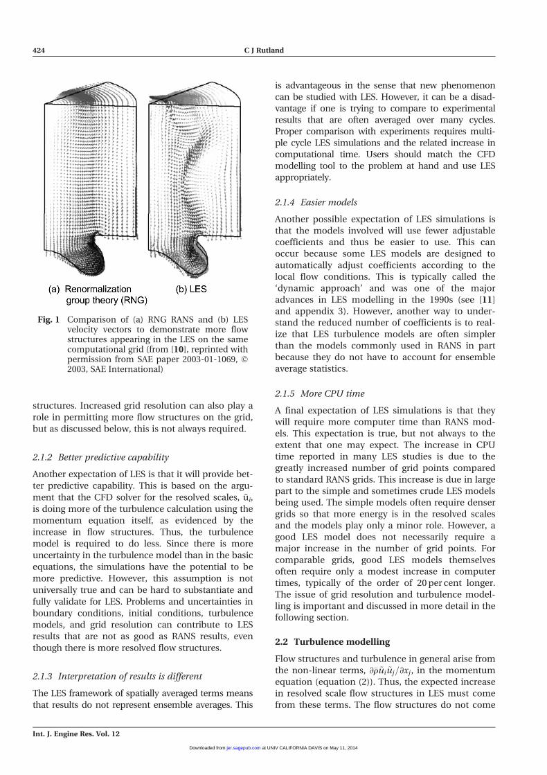
structures. Increased grid resolution can also play a

role in permitting more flow structures on the grid,

but as discussed below, this is not always required.

2.1.2 Better predictive capability

Another expectation of LES is that it will provide bet-

ter predictive capability. This is based on the argu-

ment that the CFD solver for the resolved scales, ui,

is doing more of the turbulence calculation using the

momentum equation itself, as evidenced by the

increase in flow structures. Thus, the turbulence

model is required to do less. Since there is more

uncertainty in the turbulence model than in the basic

equations, the simulations have the potential to be

more predictive. However, this assumption is not

universally true and can be hard to substantiate and

fully validate for LES. Problems and uncertainties in

boundary conditions, initial conditions, turbulence

models, and grid resolution can contribute to LES

results that are not as good as RANS results, even

though there is more resolved flow structures.

2.1.3 Interpretation of results is different

The LES framework of spatially averaged terms means

that results do not represent ensemble averages. This

is advantageous in the sense that new phenomenon

can be studied with LES. However, it can be a disad-

vantage if one is trying to compare to experimental

results that are often averaged over many cycles.

Proper comparison with experiments requires multi-

ple cycle LES simulations and the related increase in

computational time. Users should match the CFD

modelling tool to the problem at hand and use LES

appropriately.

2.1.4 Easier models

Another possible expectation of LES simulations is

that the models involved will use fewer adjustable

coefficients and thus be easier to use. This can

occur because some LES models are designed to

automatically adjust coefficients according to the

local flow conditions. This is typically called the

‘dynamic approach’ and was one of the major

advances in LES modelling in the 1990s (see [11]

and appendix 3). However, another way to under-

stand the reduced number of coefficients is to real-

ize that LES turbulence models are often simpler

than the models commonly used in RANS in part

because they do not have to account for ensemble

average statistics.

2.1.5 More CPU time

A final expectation of LES simulations is that they

will require more computer time than RANS mod-

els. This expectation is true, but not always to the

extent that one may expect. The increase in CPU

time reported in many LES studies is due to the

greatly increased number of grid points compared

to standard RANS grids. This increase is due in large

part to the simple and sometimes crude LES models

being used. The simple models often require denser

grids so that more energy is in the resolved scales

and the models play only a minor role. However, a

good LES model does not necessarily require a

major increase in the number of grid points. For

comparable grids, good LES models themselves

often require only a modest increase in computer

times, typically of the order of 20 per cent longer.

The issue of grid resolution and turbulence model-

ling is important and discussed in more detail in the

following section.

2.2 Turbulence modelling

Flow structures and turbulence in general arise from

the non-linear terms, ∂�r ~ui ~uj=∂xj, in the momentum

equation (equation (2)). Thus, the expected increase

in resolved scale flow structures in LES must come

from these terms. The flow structures do not come

Fig. 1 Comparison of (a) RNG RANS and (b) LESvelocity vectors to demonstrate more flowstructures appearing in the LES on the samecomputational grid (from [10], reprinted withpermission from SAE paper 2003-01-1069, �2003, SAE International)

424 C J Rutland




from the turbulence model. To achieve the

increased flow structures, the non-linear terms must

be allowed to function sufficiently. This can be

achieved through less dissipative turbulence models

and/or a denser grid. Both of these increase the

kinetic energy in the resolved scales so that non-

linear interactions are stronger and flow structures

are more likely to develop.

To achieve flow structures in LES, one can choose

between crude turbulence models with more grid

cells or better turbulence models with reduced grid

requirements. The choice of denser grids with

simple models is the traditional way to achieve

flow structures. However, it comes at the price of

increased computational time. The denser grid pro-

vides more resolution so that a wider range of

resolved length scales are maintained and non-

linear interactions are more likely to occur. In this

case, it is often acceptable to use simple turbulence

models since they are not required to do much

other than provide dissipation at the small scales.

As shown below, the problem is that often the mod-

els are so simple that they provide dissipation over a

wide range of length scales, and one is forced to

provide even more grid resolution to counteract this

effect.

In many situations, the number of cells in a grid

could be reduced and the grid would still be suffi-

cient for maintaining a range of length scales and

allowing non-linear interactions. However, the tur-

bulence model must allow this to happen. Simply

choosing a less dissipative but crude model often

will not work because of numerical instability. In

addition, reduced dissipation is counter to the con-

cept of LES spatial filtering in which more subgrid

dissipation should occur as the number of cells in

the grid decreases. Instead, the turbulence model

needs to improve as the number of grid cells is

reduced. An important characteristic of better LES

turbulence models are ones that let the non-linear

interactions occur while still maintaining numerical

stability.

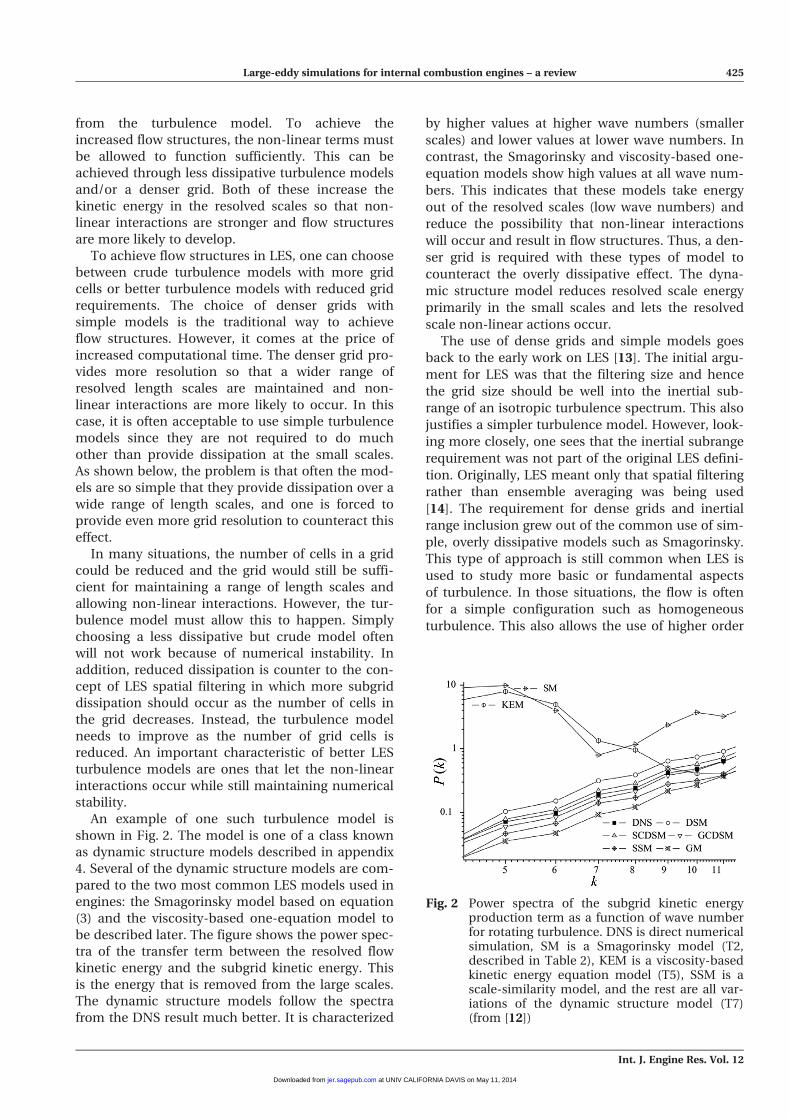
An example of one such turbulence model is

shown in Fig. 2. The model is one of a class known

as dynamic structure models described in appendix

4. Several of the dynamic structure models are com-

pared to the two most common LES models used in

engines: the Smagorinsky model based on equation

(3) and the viscosity-based one-equation model to

be described later. The figure shows the power spec-

tra of the transfer term between the resolved flow

kinetic energy and the subgrid kinetic energy. This

is the energy that is removed from the large scales.

The dynamic structure models follow the spectra

from the DNS result much better. It is characterized

by higher values at higher wave numbers (smaller

scales) and lower values at lower wave numbers. In

contrast, the Smagorinsky and viscosity-based one-

equation models show high values at all wave num-

bers. This indicates that these models take energy

out of the resolved scales (low wave numbers) and

reduce the possibility that non-linear interactions

will occur and result in flow structures. Thus, a den-

ser grid is required with these types of model to

counteract the overly dissipative effect. The dyna-

mic structure model reduces resolved scale energy

primarily in the small scales and lets the resolved

scale non-linear actions occur.

The use of dense grids and simple models goes

back to the early work on LES [13]. The initial argu-

ment for LES was that the filtering size and hence

the grid size should be well into the inertial sub-

range of an isotropic turbulence spectrum. This also

justifies a simpler turbulence model. However, look-

ing more closely, one sees that the inertial subrange

requirement was not part of the original LES defini-

tion. Originally, LES meant only that spatial filtering

rather than ensemble averaging was being used

[14]. The requirement for dense grids and inertial

range inclusion grew out of the common use of sim-

ple, overly dissipative models such as Smagorinsky.

This type of approach is still common when LES is

used to study more basic or fundamental aspects

of turbulence. In those situations, the flow is often

for a simple configuration such as homogeneous

turbulence. This also allows the use of higher order

Fig. 2 Power spectra of the subgrid kinetic energyproduction term as a function of wave numberfor rotating turbulence. DNS is direct numericalsimulation, SM is a Smagorinsky model (T2,described in Table 2), KEM is a viscosity-basedkinetic energy equation model (T5), SSM is ascale-similarity model, and the rest are all var-iations of the dynamic structure model (T7)(from [12])





numerical methods that avoided numerical

dissipation.

However, the use of very dense grids in simple

flow configurations is a more scientific use of LES

and is distinctly different from using LES in applica-

tions such as IC engines. Flows are almost never

homogeneous in applications. Traditional concepts,

such as the inertial subrange, rely on a sufficient

statistical population that often does not exist at the

smaller scale subgrid level in a complex evolving

flow. In engine applications, it is not practical to use

extremely dense grids or higher order numerical

methods. The domain size and configuration do not

allow it. In addition, the more complex physical

processes, such as combustion and sprays in

engines, require their own modelling and computa-

tional time. Thus, most practical LES applications

for engines must use coarser grids and lower order

numerics.

To account for the different types of LES, the

notation ‘scientific LES’ and ‘engineering LES’ is

introduced. Some of the characteristics of these two

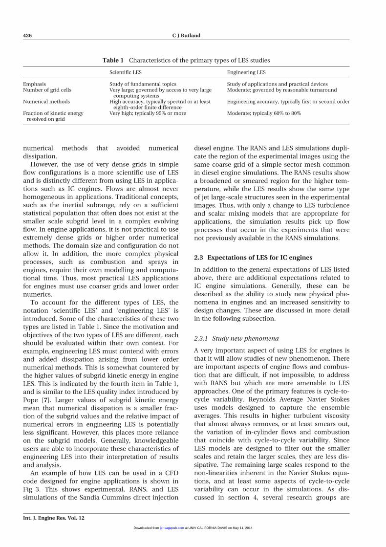
types are listed in Table 1. Since the motivation and

objectives of the two types of LES are different, each

should be evaluated within their own context. For

example, engineering LES must contend with errors

and added dissipation arising from lower order

numerical methods. This is somewhat countered by

the higher values of subgrid kinetic energy in engine

LES. This is indicated by the fourth item in Table 1,

and is similar to the LES quality index introduced by

Pope [7]. Larger values of subgrid kinetic energy

mean that numerical dissipation is a smaller frac-

tion of the subgrid values and the relative impact of

numerical errors in engineering LES is potentially

less significant. However, this places more reliance

on the subgrid models. Generally, knowledgeable

users are able to incorporate these characteristics of

engineering LES into their interpretation of results

and analysis.

An example of how LES can be used in a CFD

code designed for engine applications is shown in

Fig. 3. This shows experimental, RANS, and LES

simulations of the Sandia Cummins direct injection

diesel engine. The RANS and LES simulations dupli-

cate the region of the experimental images using the

same coarse grid of a simple sector mesh common

in diesel engine simulations. The RANS results show

a broadened or smeared region for the higher tem-

perature, while the LES results show the same type

of jet large-scale structures seen in the experimental

images. Thus, with only a change to LES turbulence

and scalar mixing models that are appropriate for

applications, the simulation results pick up flow

processes that occur in the experiments that were

not previously available in the RANS simulations.

2.3 Expectations of LES for IC engines

In addition to the general expectations of LES listed

above, there are additional expectations related to

IC engine simulations. Generally, these can be

described as the ability to study new physical phe-

nomena in engines and an increased sensitivity to

design changes. These are discussed in more detail

in the following subsection.

2.3.1 Study new phenomena

A very important aspect of using LES for engines is

that it will allow studies of new phenomenon. There

are important aspects of engine flows and combus-

tion that are difficult, if not impossible, to address

with RANS but which are more amenable to LES

approaches. One of the primary features is cycle-to-

cycle variability. Reynolds Average Navier Stokes

uses models designed to capture the ensemble

averages. This results in higher turbulent viscosity

that almost always removes, or at least smears out,

the variation of in-cylinder flows and combustion

that coincide with cycle-to-cycle variability. Since

LES models are designed to filter out the smaller

scales and retain the larger scales, they are less dis-

sipative. The remaining large scales respond to the

non-linearities inherent in the Navier Stokes equa-

tions, and at least some aspects of cycle-to-cycle

variability can occur in the simulations. As dis-

cussed in section 4, several research groups are

Table 1 Characteristics of the primary types of LES studies

Scientific LES Engineering LES

Emphasis Study of fundamental topics Study of applications and practical devicesNumber of grid cells Very large; governed by access to very large

computing systemsModerate; governed by reasonable turnaround

Numerical methods High accuracy, typically spectral or at leasteighth-order finite difference

Engineering accuracy, typically first or second order

Fraction of kinetic energyresolved on grid

Very high; typically 95% or more Moderate; typically 60% to 80%

426 C J Rutland




already making use of LES to study cycle-to-cycle

variations.

2.3.2 Increased design sensitivity

In addition, there are other flow-based processes in

engines that are best addressed with LES rather than

RANS. For example, LES should be better at captur-

ing the impact of relatively small changes in geome-

try (combustion chamber shape, pistons bowls, port

design, valve curtain regions, etc.), small changes in

fuel injection angles for direct injection applica-

tions, and small changes in operation (spark timing,

injection timing, valve timing, etc.). These types of

applications could be classified as ‘design sensitiv-

ity’ studies. Similar to cycle-to-cycle variability

applications, LES is a necessary tool for these stud-

ies due to its increased sensitivity.

Even though LES represents the next generation

of turbulence modelling, it is not always the best

choice for engine applications. The primary and

very common situation in which RANS is still the

best choice is when the desired output is a cycle-

averaged result. Obtaining a cycle-averaged result

with LES requires running several consecutive full

720 crank-angle degree cycles and averaging the

results. This can be expensive since additional grid

preparation is required for the open portions of the

cycles and computer run times are long for the ten

or more cycles required. Several research groups are

pursuing this approach (see section 4). One justifi-

cation for this more computationally expensive

approach is that LES results are more accurate so

that the average is better than a RANS result. Still,

users should evaluate their objectives and choose

the best approach, either RANS or LES.

The other significant reason that LES is at a dis-

advantage for engine applications is that many addi-

tional complex physical processes occur.

Combustion and fuel injection are probably the pri-

mary complicating processes, and these are not tri-

vial. The use of LES for turbulent combusting flows

is still a very active area of fundamental research

with many basic issues still being investigated [16].

There has been even less work in LES for liquid

sprays where one could easily argue that the physi-

cal processes are even more complex. Beyond

sprays and combustion there are complex processes

in ignition, gas phase and solid phase emissions,

boundary layers and wall heat transfer, and moving

boundaries. All of these require some sort of model-

ling that should be adapted, or at least understood,

for the LES approach.

In many situations, researchers use LES for turbu-

lence (e.g. subgrid stresses that appear in the

momentum equation) and maybe for scalar flux

modelling, but then rely on existing RANS-type sub-

models for the other physical processes. This type of

hybrid approach is very common and a very reason-

able way to proceed. Waiting until all engine sub-

models have been adapted to LES is unreasonable

and disregards the advantages that can come from

intelligent use of hybrid approaches. Since turbu-

lence is the background for most aspects of engine

flows, using LES turbulence submodels can improve

the context for the other models. The turbulence

models provide flow fields with more large-scale

structures and greater sensitivity so that many

advantages of LES can be realized, even when com-

bined with RANS models for other processes. One

could argue that there is some justification in this

approach since RANS models for combustion and

sprays should respond correctly to the resolved

large-scale flow field [17]. However, the correct

response of RANS models to the LES flow field

is not guaranteed. A user should understand the

Fig. 3 Comparison of LES (middle row) and RANS(bottom row) with experimentally imaged (toprow) ignition chemiluminescence, showing liq-uid fuel in blue and temperature in green (seescale) (from [15], reprinted with permissionfrom SAE paper 2007-01-0163, � 2007, SAEInternational)





specifics of the hybrid situation being used so that

they can better evaluate the appropriateness of the

tools for the specific study and the validity of

the results. An even better approach is to examine

the various submodels and determine if they are

consistent with the LES spatial filtering concepts

and the resulting scaling.

This brings us to the main objective of this

review, which is to report on, evaluate, and categor-

ize the use of various LES turbulence, combustion,

spray, etc., models for IC engines. Since there are

many physical processes that need modelling, there

is a wide variety of hybrid approaches in the litera-

ture that may mix-and-match various models from

these lists. Examples from the literature will be used

to illustrate some of the main categories. Then,

these categories are used to describe and classify

some of the recent uses of LES to study engines.

3 LES MODELS IN IC ENGINES

There are many complex physical processes in IC

engines, and each of these requires some sort of

modelling. These processes occur in a turbulent gas

phase flow so turbulence models, also called turbu-

lence submodels, provide the context for the other

physical processes. In addition, LES submodels

should also be used for scalar mixing, combustion,

and fuel sprays since all of these can be significan-

tly impacted by the turbulent flows. Large-eddy

simulation modelling for turbulence and these

other engine processes are discussed in the sections

below. In each case, the major modelling app-

roaches are described and classified with an empha-

sis on their suitability for engine CFD. A table is

provided in each subsection to summarize the

descriptions.

3.1 Turbulence modelling

For a quick background on turbulence modelling,

one can start from the gradient assumption used in

equation (3), although as explained below, this is

not necessarily the best approach. From equation

(3), the turbulence model is based on a turbulence

viscosity, nT, and an expression for this term is

required. As a context for the LES approach, the

most common RANS-based models use the k–epsi-

lon (k–e) approach so that

nT = Cm

k2

e(5)

The terms k and e are interpreted to be the turbu-

lent kinetic energy (TKE) and the turbulent kinetic

energy dissipation rate (or just dissipation). In mod-

ern approaches, these terms are obtained from indi-

vidual transport equations. Thus, the RANS (k–e)

model is a two-equation turbulence model.

To provide additional understanding, it is useful

to rewrite the model based on a physical interpreta-

tion using a velocity and length scale

nT = u00‘ (6)

Then, k and e provide a turbulent velocity scale

u00e ffiffiffikp

and a turbulent length scale of ‘’ ek1.5/e. In

this interpretation, the length scale is thought of as

the integral scale of the turbulence even though the

flow is not homogeneous.

If equation (3) is used for LES models, there are

several approaches for obtaining expressions for nT.

One of the more common models is based on the

ideas of Smagorinsky [18] and results in

nT = CSDð Þ2 ~S�� (7)

where |~s| measures the magnitude of the resolved

strain rate and D is a measure of the grid cell size.

Using the same physical interpretation as above,

the Smagorinsky model velocity scale is u00~D|~s| and

the length scale is the numerical grid size, D. Using

the grid size for the length scale in LES is consistent

with the LES filtering using a grid cell scale (see

appendix 2). However, it is not guaranteed that grid

size times the strain rate gives the correct velocity

scale for the LES subgrid turbulence since this is

a crude model. Usually, there are no additional

transport equations in Smagorinsky-type models so

they are zero-equation models. Variations on the

Smagorinsky model are common, and these are

described in Table 2.

Within the turbulent viscosity approach to mod-

elling, the LES model length scale is related to the

grid cell size. This means that fundamentally LES is

not grid independent. As the grid cell size becomes

smaller, an LES solution should approach a DNS

solution. This limit is well accepted and usually rea-

lized by most LES models. In contrast, as the grid

cell sizes become larger, the limit is not well estab-

lished. One possible interpretation is that the LES

model length scale should approach a RANS model

integral scale. However, this is not observed in prac-

tice and, pragmatically, it is inadvisable to use LES

models on grids coarser than ones used in RANS.

Even though most turbulence models use some

form of equation (3), it can be argued that it is not

the best type of model for LES for three important

reasons.

428 C J Rutland




1. Overly dissipative. As discussed in the previous

sections, this approach can be overly dissipative.

2. No subgrid kinetic energy. In equation (3) type

models for LES, the subgrid TKE is arbitrary. This

is because the trace of the subgrid stress tensor,

tii, is twice the kinetic energy, but the trace of the

strain rate tensor is zero in incompressible flows.

This is why equation (3) uses the anisotropic part

of the subgrid stress tensor, trij. In engine flows,

the subgrid kinetic energy is a very important

variable for additional models in combustion,

scalar mixing, and sprays. Thus, an additional

model must be formulated for the subgrid kinetic

energy. These models are commonly very simple,

ad hoc, and poorly justified [19].

3. Incorrect tensor relationship. Fundamentally,

equation (3) assumes the tensor relationship

bet-ween trij and is valid. Specifically, equation

(3) assumes the principle directions of trij and ~sij

align. This is known to be incorrect [14], and

indicates a basic problem with the Boussinesq

assumption embodied by equation (3). There

are LES models that do not use equation (3),

and these may offer advantages for LES in

engine applications. These are described in

appendix 4 and Table 2.

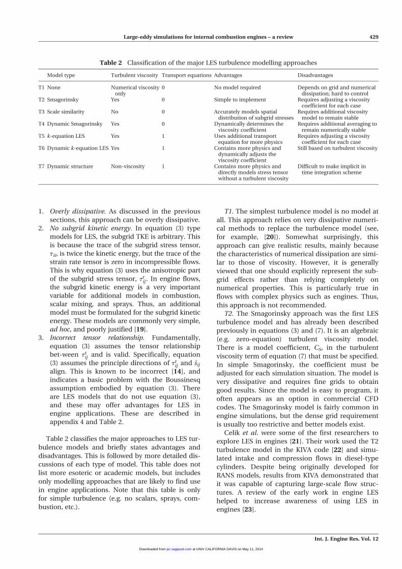
Table 2 classifies the major approaches to LES tur-

bulence models and briefly states advantages and

disadvantages. This is followed by more detailed dis-

cussions of each type of model. This table does not

list more esoteric or academic models, but includes

only modelling approaches that are likely to find use

in engine applications. Note that this table is only

for simple turbulence (e.g. no scalars, sprays, com-

bustion, etc.).

T1. The simplest turbulence model is no model at

all. This approach relies on very dissipative numeri-

cal methods to replace the turbulence model (see,

for example, [20]). Somewhat surprisingly, this

approach can give realistic results, mainly because

the characteristics of numerical dissipation are simi-

lar to those of viscosity. However, it is generally

viewed that one should explicitly represent the sub-

grid effects rather than relying completely on

numerical properties. This is particularly true in

flows with complex physics such as engines. Thus,

this approach is not recommended.

T2. The Smagorinsky approach was the first LES

turbulence model and has already been described

previously in equations (3) and (7). It is an algebraic

(e.g. zero-equation) turbulent viscosity model.

There is a model coefficient, CS, in the turbulent

viscosity term of equation (7) that must be specified.

In simple Smagorinsky, the coefficient must be

adjusted for each simulation situation. The model is

very dissipative and requires fine grids to obtain

good results. Since the model is easy to program, it

often appears as an option in commercial CFD

codes. The Smagorinsky model is fairly common in

engine simulations, but the dense grid requirement

is usually too restrictive and better models exist.

Celik et al. were some of the first researchers to

explore LES in engines [21]. Their work used the T2

turbulence model in the KIVA code [22] and simu-

lated intake and compression flows in diesel-type

cylinders. Despite being originally developed for

RANS models, results from KIVA demonstrated that

it was capable of capturing large-scale flow struc-

tures. A review of the early work in engine LES

helped to increase awareness of using LES in

engines [23].

Table 2 Classification of the major LES turbulence modelling approaches

Model type Turbulent viscosity Transport equations Advantages Disadvantages

T1 None Numerical viscosityonly

0 No model required Depends on grid and numericaldissipation; hard to control

T2 Smagorinsky Yes 0 Simple to implement Requires adjusting a viscositycoefficient for each case

T3 Scale similarity No 0 Accurately models spatialdistribution of subgrid stresses

Requires additional viscositymodel to remain stable

T4 Dynamic Smagorinsky Yes 0 Dynamically determines theviscosity coefficient

Requires additional averaging toremain numerically stable

T5 k-equation LES Yes 1 Uses additional transportequation for more physics

Requires adjusting a viscositycoefficient for each case

T6 Dynamic k-equation LES Yes 1 Contains more physics anddynamically adjusts theviscosity coefficient

Still based on turbulent viscosity

T7 Dynamic structure Non-viscosity 1 Contains more physics anddirectly models stress tensorwithout a turbulent viscosity

Difficult to make implicit intime integration scheme





An additional variation associated with T2 type

models was developed by Nicoud and Ducros [24]

and called wall adapting local eddy (WALE) viscos-

ity. This replaces the strain rate magnitude in the

turbulent viscosity in equation (7) by a more com-

plex tensor contraction of the strain rate and velo-

city gradient tensor. There is some indication WALE

has better near-wall performance so that grid

requirements can be reduced, but this needs further

investigation. Poinsot, with a variety of other

researchers, has used WALE with non-engine flows

in the development of a new code for engine appli-

cations [25, 26]. Bianchi et al. have shown good

results with WALE in engine flows with a detailed

analysis of flow around the intake valves [27, 28].

T3. The scale-similarity modelling approach was

originally proposed by Bardina et al. [29], and is

explained in more depth by Meneveau and Katz

[30]. The concept is that unresolved subgrid scales

can be approximated by the smallest resolved

scales. In other words, the best way to represent

subgrid scales is with the next largest scales. This

approach is implemented by using an additional

spatial filtering operation on the already filtered

scales. The additional filtering may be called a test

filter in some approaches and is indicated by an

additional overbar-type symbol (see appendix 3).

Scale-similarity is an important concept in LES

and does not occur in RANS modelling. The original

approach is usually unstable, mainly because it is

not a viscosity model and does not use an energy

budget to track the subgrid kinetic energy. Thus, the

scale-similarity model is usually augmented by the

addition of a Smagorinsky term in what is termed a

hybrid model.

The Lund University group has been exploring

LES for engines for several years using a scale-simi-

larity model for turbulence. A lot of their work is

focused on homogeneous charge compression igni-

tion (HCCI) combustion, and is reviewed in section

4. They worked with Paul Miles from the

Combustion Research Facility at Sandia National

Labs to make detailed comparisons of motored in-

cylinder velocity fields [31]. They used dense grids,

and the comparisons between the LES and the PIV

are reasonable. Interestingly, the work demonstrates

the difficulty in validating the LES.

T4. A major improvement in the Smagorinsky

approach occurred when the dynamic approach

was developed by Germano et al. [11]. In this

approach, the adjustable coefficient, Cs, in equation

(7) is obtained using the dynamic procedure. The

dynamic procedure uses the scale-similarity con-

cept of T3 that requires an additional spatial filter-

ing step. The dynamic coefficient is found from the

difference between these additionally filtered quan-

tities and the base quantities calculated on the CFD

grid (see appendix 3). This additional filtering oper-

ation is a modest increase in computational cost,

resulting in an increase of ~20 per cent for a simple

turbulent flow.

An interesting variation of the dynamic procedure

was developed by Meneveau et al. [32], in which a

Lagrangian concept was used to develop the model

coefficient. The idea was to average over fluid parti-

cle pathlines to improve accuracy. In practice, two

additional transport equations were used to repre-

sent the Lagrangian average of terms used to evalu-

ate the dynamic coefficient.

Haworth et al. were also some of the early

explorers in using LES for IC engines [33]. They

mostly used T2 and T4 type models in several differ-

ent codes. They carried out extensive studies on a

simple, engine type flow with a stationary valve [34].

This configuration, sometimes called the Imperial

College engine, has a large experimental dataset and

is useful for validating valve flows. Haworth et al.

have shown good comparison between ensemble

averaged LES models and experimental data for

both mean and fluctuating velocity profiles at differ-

ent locations and different crank angles.

The dynamic procedure is very powerful and can

be used in many situations to find modelling coeffi-

cients. When used with the Smagorinsky model, the

results are reasonably good for non-reacting flows.

However, dense grids are required and often an

additional averaging must be used to avoid instabil-

ities that arise from negative viscosities. Despite the

improvements found in T4, it still retains the draw-

backs of the equation (3) viscosity models discussed

in the previous section. No matter how good a

model is formulated for the turbulent viscosity, the

fundamentals of T2 and T4 are very weak.

T5. The k-equation approach is a practical viscos-

ity-based, one-equation LES model. It was originally

developed for atmospheric flows [35], and is still

common in that field. Some of the first useful

k-equation models for engineering flows were devel-

oped by Kim and Menon [36]. This model was still

viscosity based (equation (3)), but now the turbulent

viscosity was formed from the subgrid TKE, ksgs, and

a grid length scale, D, resulting in the following

expression

nT = CkD

ffiffiffiffiffiffiffiffiksgs

q(8)

The subgrid TKE was obtained from an additional

transport equation that was readily derived from the

basic equations. The use of the k transport equation

430 C J Rutland




has several distinct advantages. First, it incorpo-

rates more physical processes, such as the convec-

tion, production, and dissipation of subgrid kinetic

energy. Second, the subgrid kinetic energy provides

a velocity scaling that can be used in other models,

such as combustion, scalar transport, and sprays.

Third, models that use a subgrid k-equation provide

a better model for the subgrid stresses and thus

work better on the coarser grids commonly found in

engine CFD [37, 38].

Menon et al. have applied the T5 turbulence

model to engine flows with good results [39].

Bianchi et al. have performed careful studies of LES

models for engine type flows in simple configura-

tions. For example, they have compared T2 and T5

turbulence models with RANS results for a station-

ary valve, steady flow bench configuration [28].

The subgrid kinetic energy equation is fairly sim-

ple to implement. It requires only one additional

major modelled term, which is for the dissipation of

subgrid kinetic energy. Fortunately, this term plays

its proper role in LES, which at the subgrid scale is

to remove kinetic energy. The dissipation term is

not required to provide the mean value for all scales,

nor is it used to obtain length scales or time scales

as it is in RANS modelling. Thus, dissipation model-

ling is much less critical, and simple models seem

to work well.

T6. The k-equation LES models have also been

implemented using the dynamic procedure to

obtain a better, local value for the coefficient in

equation (8) [36]. This method is a logical extension

of T5; however, additional implementation details

must be observed to maintain stability. At this time,

it is not clear if this additional complexity beyond

the basic T5 model is useful in engine simulations.

T7. A recent development in LES turbulence mod-

els is the dynamic structure approach developed by

Pomraning and Rutland [40] and Chumakov and

Rutland [41]. In this approach, a turbulent viscosity

is not used. Instead, a tensor coefficient is obtained

directly from the dynamic procedure. This tensor

coefficient is multiplied by the TKE that is obtained

from a transport equation (see appendix 4 for more

details). The resulting dynamic structure model is

tij = Cijksgs (9)

An important major aspect of the dynamic structure

approach is that there is no turbulent viscosity.

Thus, it is not a purely dissipative model. Instead, a

budget of TKE is maintained between the grid scale

velocity field and the subgrid k-equation. In other

words, energy removed from the grid scales

goes into the subgrid kinetic energy. Then, within

the k-equation, a viscous dissipation term removes

the energy through molecular viscosity. Detailed a

priori and a posteriori testing of the model has

shown it performs well in rotating turbulence in

which energy is transferred accurately from small to

large scales, a process that is similar to that occur-

ring in sprays and combustion systems [12, 42].

The model was developed for practical applica-

tions, especially IC engines, in which the number of

grid cells must remain reasonable. The model works

very well in engine applications, and provides a

good model for the subgrid TKE for use in combus-

tion, scalar mixing, and spray models. The T7

approach has been used for diesel engine simula-

tions with good results [15, 43, 44].

3.1.1 Turbulence: additional considerations

Wall boundary conditions. Wall boundary condi-

tions for LES submodels are not very well devel-

oped. There has been continued effort is this area

for several years (e.g. Kannepalli and Piomelli [45]

and Chang et al. [46]), but, to date, no significant

progress has been made on practical models for

CFD applications. Some promising advanced work

by Cabot and Moin [47] used RANS models with

additional consideration for unsteadiness and ‘ejec-

tion’ events. However, these have only been used on

simple channel flows and will probably require

much more additional testing before they can be

used with confidence in applications. More recently

Piomelli [48] has reviewed the status of wall model-

ling for LES, and Frohlich and von Terzi [49] dis-

cussed combining LES with RANS wall models.

Thus, most LES simulations use one of two

approaches for wall boundary conditions: (a) no

special treatment of the wall, except for additional

grid points (Kannepalli and Piomelli [45]), and (b)

wall-layer models essentially the same as used in

RANS that have been shown, by Rodi et al. [50], to

give reasonably good results. For engine applica-

tions, the use of wall functions is probably the best

approach for the near future. This is especially true

when one considers wall heat transfer for which

there has been essentially no work on engines for

LES specific wall models.

Higher order numerics. In simulations that are

less focused on applications and more focused on

generic flows, such as channels and isotropic turbu-

lence, numerical accuracy is an important issue

[51]. The concern is that numerical errors could be

of the same order as the LES modelled terms. The

generic flows commonly use higher order spatial

numerics, typically fourth order or higher. In addi-

tion to being higher order, the methods have low





dispersion and dissipation errors. This is possible

because the computational domains are simple and

the grids allow easy implementation of higher order

numerics. In contrast, applications such as IC

engines commonly have complex grids and it is very

difficult to achieve anything higher than second-

order spatial accuracy. This should not and has not

deterred the use of LES to achieve better results in

engine applications.

There has been encouraging work by the group at

Doshisha University to improve the numerical accu-

racy in the KIVA engine applications code [52, 53].

This work correctly focuses on the advection or con-

vection term in the momentum equation and has

compared several numerical methods, including

one that is up to third-order accurate. The results

are encouraging, but have only been demonstrated

on simple grids in the engine code and have not

been demonstrated on grids for actual engine

configurations.

Another tactic for higher order accuracy is being

used by Poinsot et al. at IFP and CERFACS, in which

an existing LES code developed for aeronautical

applications is being adapted for IC engines [25,

54]. The code is known as AVBP, and has second-

order time accuracy and third-order spatial accu-

racy on the convection terms. The time integration

scheme is explicit, which offers higher accuracy

than an implicit scheme since the time step is

restricted to smaller values. Adaption for engines is

not straightforward, but moving mesh algorithms

have been implemented; however, grid removal

does not seem to be included yet. The code is being

carefully tested and is showing good results for

engine applications [55].

Compressibility effects. Even though the gas den-

sity varies significantly in engines, they are generally

considered low Mach number regimes [56]. Thus,

pressure wave effects on turbulence modelling are

almost never considered. The exception is when

engine knock or extremely rapid ignition occurs.

While some HCCI operation is similar to knock, it

can be considered a different mechanism that is

probably not a consequence of pressure waves in

most cases. There are many RANS-based studies of

knock (see, for example, [57]) but there does not

appear to be any LES studies yet. This will probably

change before long as ‘mega knock’ in downsized

[58] or direct injection gasoline engines is studied.

Open boundary conditions. Many engine studies

are focused on the closed portion of the cycle and

thus avoid open boundaries. However, as multicycle

simulations become more common to study topics

such as cycle-to-cycle variability, inflow and outflow

boundary conditions must be considered. It is not

always clear what information should be specified

on the boundaries to achieve accurate simulations.

One LES study found that boundary flow perturba-

tions can have a significant impact on combustion

[59]. This topic needs additional study, and it is

likely that the type of engine, the specific models

being used, and the focus of the investigation will

have an impact on what boundary conditions are

required.

3.1.2 Turbulence: recommendations

1. The use of LES for basic turbulence modelling in

applications is becoming better established and

can be used for engine CFD with the appropriate

models.

2. The most common LES models use simple visc-

osity formulations (T2, T4) and do not take

advantage of LES concepts. They require high

grid resolution, which can be achieved using

highly parallel codes.

3. The more advanced differential LES turbulence

models (T5–T7) should be used. These do not

require extremely fine grids and work well on

the grids commonly found in engine

applications.

4. Models that use a subgrid TKE, ksgs, are well sui-

ted to engines because this term can be used in

modelling combustion, scalar mixing, and

sprays.

3.2 Combustion modelling

The phrase ‘combustion modelling’ refers to model-

ling the chemical reaction rate terms in the energy

and species conversation equations. Often, these

models incorporate additional transport equations

for mixture fraction or flame surface expressions.

These additional equations may require additional

models for terms such as scalar dissipation or tur-

bulent flame speeds. Combustion modelling is a

complex and evolving field. Readers should consult

reviews by Pitsch [16], Menon [60], Veynante and

Vervish [61], Hilbert et al. [62], and the book by

Poinsot and Veynante [8] for detailed background

information. In this section, the major combustion

models that are used or have potential application

for IC engine CFD are classified and briefly

described.

In almost all cases, the combustion models are

essentially RANS models that have been or could be

adapted for use in LES. This approach clearly treats

LES as an evolution of RANS modelling and seems

432 C J Rutland




to work well. The combustion models benefit from

the LES flow field and scalar mixing models. In

addition, as noted by Kempf et al. [17], the RANS

formulations, though originally based on ensemble

averaging, may still be appropriate for LES-based

spatial averaging and respond correctly to the

LES flow field. However, the best approach is to re-

evaluate the models and make appropriate modifi-

cations to be consistent with the LES approach. This

adaptation may be as simple as adjusting coeffi-

cients within the original RANS model. Or they may

be more complex and require reformulation of the

expressions to be consistent with the time scales

that are available from the LES turbulence and mix-

ing models. For example, specific LES formulations

of scalar dissipation models may be required in

mixture-fraction-based combustion models (see, for

example, [63]).

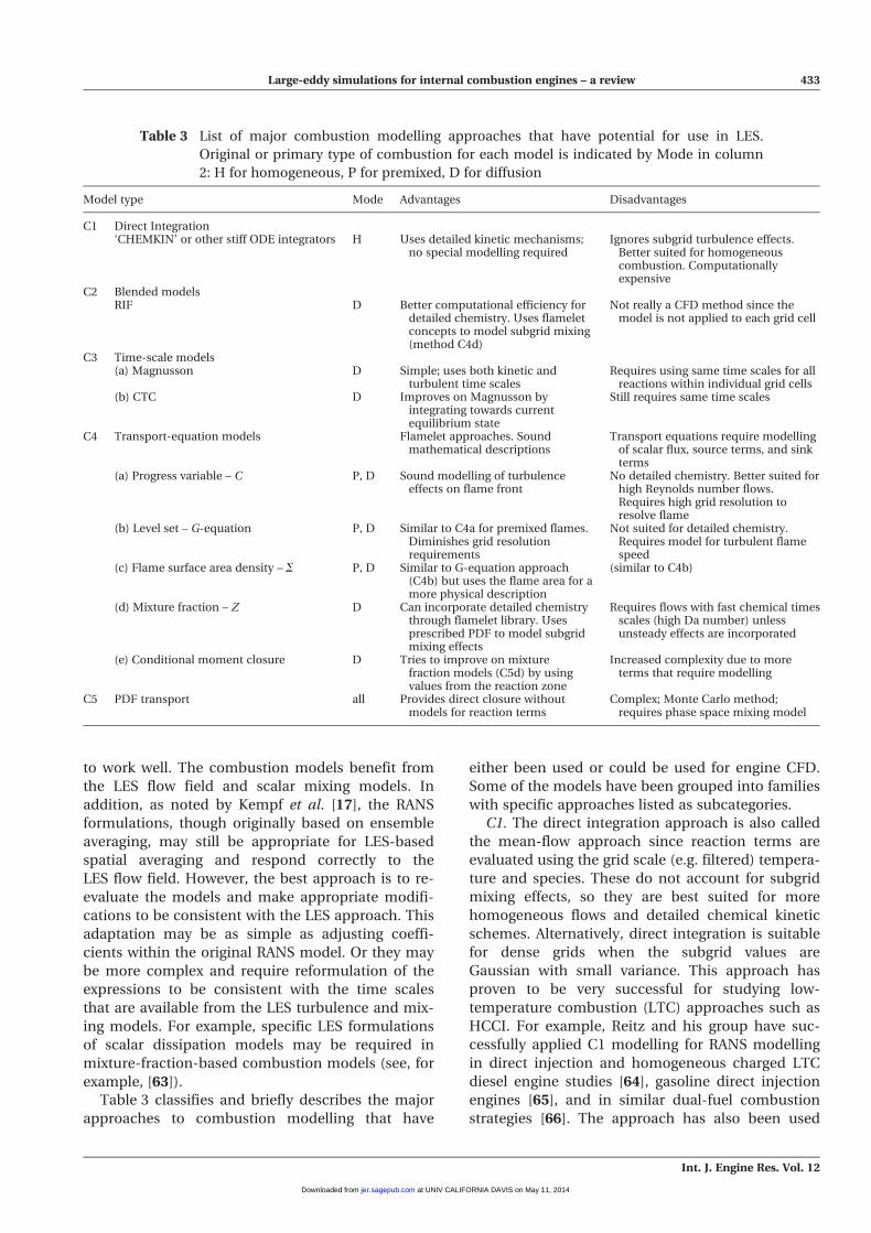
Table 3 classifies and briefly describes the major

approaches to combustion modelling that have

either been used or could be used for engine CFD.

Some of the models have been grouped into families

with specific approaches listed as subcategories.

C1. The direct integration approach is also called

the mean-flow approach since reaction terms are

evaluated using the grid scale (e.g. filtered) tempera-

ture and species. These do not account for subgrid

mixing effects, so they are best suited for more

homogeneous flows and detailed chemical kinetic

schemes. Alternatively, direct integration is suitable

for dense grids when the subgrid values are

Gaussian with small variance. This approach has

proven to be very successful for studying low-

temperature combustion (LTC) approaches such as

HCCI. For example, Reitz and his group have suc-

cessfully applied C1 modelling for RANS modelling

in direct injection and homogeneous charged LTC

diesel engine studies [64], gasoline direct injection

engines [65], and in similar dual-fuel combustion

strategies [66]. The approach has also been used

Table 3 List of major combustion modelling approaches that have potential for use in LES.

Original or primary type of combustion for each model is indicated by Mode in column

2: H for homogeneous, P for premixed, D for diffusion

Model type Mode Advantages Disadvantages

C1 Direct Integration‘CHEMKIN’ or other stiff ODE integrators H Uses detailed kinetic mechanisms;

no special modelling requiredIgnores subgrid turbulence effects.

Better suited for homogeneouscombustion. Computationallyexpensive

C2 Blended modelsRIF D Better computational efficiency for

detailed chemistry. Uses flameletconcepts to model subgrid mixing(method C4d)

Not really a CFD method since themodel is not applied to each grid cell

C3 Time-scale models(a) Magnusson D Simple; uses both kinetic and

turbulent time scalesRequires using same time scales for all

reactions within individual grid cells(b) CTC D Improves on Magnusson by

integrating towards currentequilibrium state

Still requires same time scales

C4 Transport-equation models Flamelet approaches. Soundmathematical descriptions

Transport equations require modellingof scalar flux, source terms, and sinkterms

(a) Progress variable – C P, D Sound modelling of turbulenceeffects on flame front

No detailed chemistry. Better suited forhigh Reynolds number flows.Requires high grid resolution toresolve flame

(b) Level set – G-equation P, D Similar to C4a for premixed flames.Diminishes grid resolutionrequirements

Not suited for detailed chemistry.Requires model for turbulent flamespeed

(c) Flame surface area density – S P, D Similar to G-equation approach(C4b) but uses the flame area for amore physical description

(similar to C4b)

(d) Mixture fraction – Z D Can incorporate detailed chemistrythrough flamelet library. Usesprescribed PDF to model subgridmixing effects

Requires flows with fast chemical timesscales (high Da number) unlessunsteady effects are incorporated

(e) Conditional moment closure D Tries to improve on mixturefraction models (C5d) by usingvalues from the reaction zone

Increased complexity due to moreterms that require modelling

C5 PDF transport all Provides direct closure withoutmodels for reaction terms

Complex; Monte Carlo method;requires phase space mixing model





successfully in LES applications using the T7 turbu-

lence model for direct injection diesel LTC studies

by Rutland and his group [15, 43, 44].

The C1 approach requires detailed chemical

kinetic mechanisms to be successful in engines, and

this usually results in very large computational run

times. Progress in improving run times is being

achieved by improved load balancing in parallel

computing environments [67]. Additional run-time

improvements are being achieved by applying

advanced numerical techniques such as cell cluster-

ing and analytical Jacobians [68] or precomputed,

tabulated results from detailed chemistry calcula-

tions [69, 70]. These methods are computationally

efficient, but may require close monitoring of

approximation errors, especially for ignition and

other situations where results are sensitive to kinetic

details.

C2. In an attempt to incorporate more detailed

chemical kinetics but without the computational

penalty, Peters’ group have developed the represen-

tative interactive flamelet (RIF) model [71–74].

Individual ‘flamelets’ that represent the main com-

bustion process are tracked using a Lagrangian

method through the domain. The approach can be

calibrated to work with conventional diesel combus-

tion and provide detailed chemistry for emissions.

However, the approach has difficulty with more

homogeneous flows, wall heat transfer, multiple fuel

injection operation, and spatially non-uniform

mixing that can occur in different regions of the

combustion chamber. Additional flamelets are

sometimes added to help address these issues, and

the method begins to resemble the cell clustering

approach used in C1 models. Combustion is tracked

by the Lagrangian flamelets rather than the pro-

cesses within each CFD grid cell. The approach is

more of a blending between a CFD flow model and

a system level heat-release model. Since it is not

clear how a representative flamelet concept is con-

sistent with the LES spatial filtering approach, the

RIF approach is not recommended for LES.

C3. For RANS applications, the time-scale

approach was originally developed for spark ignition

engines (Abraham et al. [75]) and later adapted for

diesel engines (Kong and Reitz [76]). The character-

istic time-scale (CTC) model is a very practical

approach that can give good results when experi-

mental data are available to adjust coefficients. The

CTC model is an outgrowth of the less commonly

used Magnusson type approaches, but is more

advanced in that CTC drives species concentrations

to a specified value. This specified value is com-

monly the local equilibrium value. However, in

some models this specified value is obtained from a

strained laminar flamelet solution (see, for example,

Rao and Rutland [77]). This effectively combines the

flamelet-prescribed PDF approach (C4d) with the

time-scale approach and has been used successfully

with LES turbulence models in diesel engine simula-

tions [78].

C4a. The flame-sheet approximation for premixed

flames has been developed in two formulations: the

C-equation and the G-equation approaches origi-

nally developed by Bray [79] and Kerstein et al. [80],

respectively. However, as shown by Zimont [81], the

approaches are very similar. In the C-equation

approach, the RANS flame brush is represented by

a progress variable C (commonly normalized

temperature). This flame-sheet approach has been

extended by Zimont et al. [82] for RANS

simulations.

The group at the Lund University has published

a series of papers using a progress variable

approach with a very highly resolved T2 turbulence

model [31, 83–85]. Their work was focused on

understanding HCCI and they achieved good com-

parisons with experimental pressure traces.

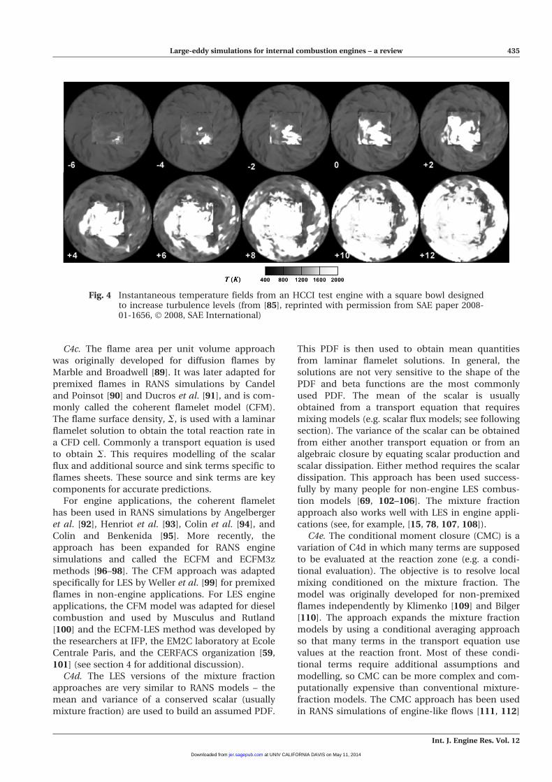
Figure 4 shows an example from one of their LES

simulations. Additional discussion of their work

appears in section 4.

The adaptation of the C progress variable model

for LES has shifted away from the RANS moment-

based approaches towards a simpler formulation

called the thickened flame model [86]. This is a sim-

ple concept that artificially increases the flame

thickness and is motivated by reducing the com-

putational time used in the combustion model.

This allows denser grids and more resolved scale

motions that work well with the thickened flame.

Researchers in France have made good use of this

approach in LES and have simulated multiple cycles

of a spark ignited premixed charge compression

ignition (PCCI) engine [55].

C4b. The G-equation approach uses a continuous

variable, G, but assumes that a specific line of con-

stant G represents the flame front. It is a level-set,

kinematically based approach and is extended to

combustion only by the concept of a flame sheet.

The function G evolves by a standard transport

equation that requires models for the subgrid sca-

lar flux. This approach is being developed for RANS

simulations (see summary in Peters [87]). It also

shows some promise for use in LES simula-

tions of premixed flames [88]. More recently the

G-equation approach has been formulated for dif-

fusion flames and used in diesel engine simulations

by Yang and Reitz [65]. These simulations use

RANS modelling, but the extension to LES should

be straightforward.

434 C J Rutland




C4c. The flame area per unit volume approach

was originally developed for diffusion flames by

Marble and Broadwell [89]. It was later adapted for

premixed flames in RANS simulations by Candel

and Poinsot [90] and Ducros et al. [91], and is com-

monly called the coherent flamelet model (CFM).

The flame surface density, S, is used with a laminar

flamelet solution to obtain the total reaction rate in

a CFD cell. Commonly a transport equation is used

to obtain S. This requires modelling of the scalar

flux and additional source and sink terms specific to

flames sheets. These source and sink terms are key

components for accurate predictions.

For engine applications, the coherent flamelet

has been used in RANS simulations by Angelberger

et al. [92], Henriot et al. [93], Colin et al. [94], and

Colin and Benkenida [95]. More recently, the

approach has been expanded for RANS engine

simulations and called the ECFM and ECFM3z

methods [96–98]. The CFM approach was adapted

specifically for LES by Weller et al. [99] for premixed

flames in non-engine applications. For LES engine

applications, the CFM model was adapted for diesel

combustion and used by Musculus and Rutland

[100] and the ECFM-LES method was developed by

the researchers at IFP, the EM2C laboratory at Ecole

Centrale Paris, and the CERFACS organization [59,

101] (see section 4 for additional discussion).

C4d. The LES versions of the mixture fraction

approaches are very similar to RANS models – the

mean and variance of a conserved scalar (usually

mixture fraction) are used to build an assumed PDF.

This PDF is then used to obtain mean quantities

from laminar flamelet solutions. In general, the

solutions are not very sensitive to the shape of the

PDF and beta functions are the most commonly

used PDF. The mean of the scalar is usually

obtained from a transport equation that requires

mixing models (e.g. scalar flux models; see following

section). The variance of the scalar can be obtained

from either another transport equation or from an

algebraic closure by equating scalar production and

scalar dissipation. Either method requires the scalar

dissipation. This approach has been used success-

fully by many people for non-engine LES combus-

tion models [69, 102–106]. The mixture fraction

approach also works well with LES in engine appli-

cations (see, for example, [15, 78, 107, 108]).

C4e. The conditional moment closure (CMC) is a

variation of C4d in which many terms are supposed

to be evaluated at the reaction zone (e.g. a condi-

tional evaluation). The objective is to resolve local

mixing conditioned on the mixture fraction. The

model was originally developed for non-premixed

flames independently by Klimenko [109] and Bilger

[110]. The approach expands the mixture fraction

models by using a conditional averaging approach

so that many terms in the transport equation use

values at the reaction front. Most of these condi-

tional terms require additional assumptions and

modelling, so CMC can be more complex and com-

putationally expensive than conventional mixture-

fraction models. The CMC approach has been used

in RANS simulations of engine-like flows [111, 112]

Fig. 4 Instantaneous temperature fields from an HCCI test engine with a square bowl designedto increase turbulence levels (from [85], reprinted with permission from SAE paper 2008-01-1656, � 2008, SAE International)





and in diesel engines [113]. The CMC approach has

been adapted to LES for non-engine flows (see, for

example, Steiner and Bushe [114]), but it is not

straightforward, as shown by Triantafyllidis and

Mastorakos [115]. Generally, results with CMC are

usually slightly better than a typical C4d model.

However, the CMC complexity and lack of general

experience that comes from wider use indicate that

the approach still needs development for use in LES

of complex engine flows.

C5. An additional combustion modelling

approach is based on the PDF evolution equation

models. The approach is often referred to as the

‘transported PDF’ approach as opposed to the ‘pre-

sumed PDF’ approach in C4d and C4e. The theory

was originally developed by Pope [116], primarily

for RANS environments. A recent review of this

method by Haworth [117] provides detailed infor-

mation about the physics, mathematics, and

numerical details of this approach, including a sec-

tion on its use for engines. This is a complex

approach using Monte-Carlo methods to track the

evolution of the underlying PDFs that describe the

thermal and, in some cases, velocity fields. The pri-

mary advantage of the approach is that it does not

require any additional models for the chemical reac-

tion terms. However, it does require models for sub-

grid turbulence and phase space mixing. The

method is so different from the other approaches

discussed here that some users find it difficult to

use. Since it is a statistical approach, the method

can require long CPU run times. However,

Subramaniam and Haworth [118] and Kung and

Haworth [119] are actively developing the method

for IC engine application and are achieving good

results in RANS simulations. There is little LES work

with the transported PDF approach and there does

not appear to be any published applications of the

models to LES engine simulations to date.

3.2.1 Combustion: additional considerations

Time scales. Combustion models in LES require

good models for mixing of species and/or thermal

energy. Large-eddy simulation is well suited to pro-

vide better mixing information in support of com-

bustion models, especially at the grid scale. At the

subgrid scale, combustion models require time-

scale information in one form or another (mixing

times, scalar dissipation, kinetic times, etc.).

Currently, LES models are less well suited to this

task because there has been less development on

models that provide this information. Often, subgrid

time-scale information is obtained from turbulent

viscosity and local mean gradients, but this is based

on RANS concepts. The newer one-equation turbu-

lence models (T5, T6, T7) are better at providing

time-scale information because they track the sub-

grid kinetic energy ksgs using a transport equation.

This can be combined with length scales (gradients

or filter length scales) to provide time scales to com-

bustion models.

Multimode combustion. In some engine appli-

cations, combustion does not easily fall into the

traditional classifications of premixed mode or

non-premixed mode. Or combustion may occur in

multiple modes within a cycle. Examples are direct

injection gasoline technologies and some of the

newer LTC technologies such as partially PCCI.

These types of combustion processes are probably

best described by combinations of direct integration

for ignition (C1), premixed and partially premixed

combustion for early, more highly mixed processes

(C3, C4a–c), and mixing controlled combustion for

later processes (C4d–e). These multimode opera-

tions can occur in a time sequence, or simultane-

ously, but in different regions in the combustion

chamber, or some combination of these two situa-

tions. A combination C4a and C4d model for non-

engine LES was reported by Ihme and Pitsch [120].

For engine applications, hybrid approaches have

been explored for RANS diesel applications [107]

and premixed/diffusion combustion in the ECFM3Z

model [95]. More recent work has demonstrated

LES simulations of diesel engine simulations using a

combination of C1, C3b, and C4d combustion mod-

els with a T7 turbulence model [15, 44].

The difficulty with multimode approaches is des-

ignating and accurately evaluating the best para-

meters for switching between the modes.

Commonly, these parameters measure a mixing

state (for example scalar dissipation rate), relative

timescales (Damkohler or Karlovitz numbers), or

reaction progress (for example, reaction products or

normalized temperature). Currently, there is not a

good theoretical framework for determining the

switching parameters, so they are often developed

based on physical arguments. In addition, the

switching procedure and the value at which

the switch occurs may have a greater impact on the

results than the details of the individual combustion

models. Clearly, much more work needs to be done

in this area for both RANS and LES modelling.

3.2.2 Combustion: recommendations

1. Use transport-based combustion models (C4).

The transport equations in these models benefit

436 C J Rutland




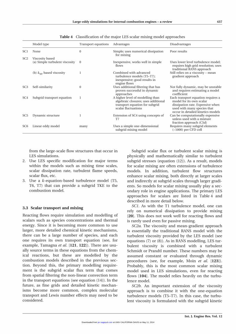
from the large-scale flow structures that occur in

LES simulations.

2. Use LES specific modification for major terms

within the models such as mixing time scales,

scalar dissipation rate, turbulent flame speeds,

scalar flux, etc.

3. Use a k-equation-based turbulence model (T5,

T6, T7) that can provide a subgrid TKE to the

combustion model.

3.3 Scalar transport and mixing

Reacting flows require simulation and modelling of

scalars such as species concentrations and thermal

energy. Since it is becoming more common to use

larger, more detailed chemical kinetic mechanisms,

there can be a large number of species, and each

one requires its own transport equation (see, for

example, Tamagna et al. [121, 122]). There are usu-

ally source terms in these equations from the chem-

ical reactions, but these are modelled by the

combustion models described in the previous sec-

tion. Beyond this, the primary modelling require-

ment is the subgrid scalar flux term that comes

from spatial filtering the non-linear convection term

in the transport equations (see equation (14)). In the

future, as fine grids and detailed kinetic mechan-

isms become more common, complex molecular

transport and Lewis number effects may need to be

considered.

Subgrid scalar flux or turbulent scalar mixing is

physically and mathematically similar to turbulent

subgrid stresses (equation (12)). As a result, models

for scalar mixing are often extensions of turbulence

models. In addition, turbulent flow structures

enhance scalar mixing, both directly at larger scales

and indirectly at subgrid scales through larger gradi-

ents. So models for scalar mixing usually play a sec-

ondary role in engine applications. The primary LES

approaches for scalars are listed in Table 4 and

described in more detail below.

SC1. As with the T1 turbulence model, one can

rely on numerical dissipation to provide mixing

[20]. This does not work well for reacting flows and

is rarely used even for passive mixing.

SC2a. The viscosity and mean-gradient approach

is essentially the traditional RANS model with the

turbulent viscosity provided by the LES model (see

equations (7) or (8)). As in RANS modelling, LES tur-

bulent viscosity is combined with a turbulent

Schmidt or Prandtl number. These numbers may be

assumed constant or evaluated through dynamic

procedures (see, for example, Moin et al. [123]).

Probably, this is the most common scalar mixing

model used in LES simulations, even for reacting

flows [104]. The model relies heavily on the turbu-

lence model.

SC2b. An important extension of the viscosity

approach is to combine it with the one-equation

turbulence models (T5–T7). In this case, the turbu-

lent viscosity is formulated with the subgrid kinetic

Table 4 Classification of the major LES scalar mixing model approaches

Model type Transport equations Advantages Disadvantages

SC1 None 0 Simple; uses numerical dissipationfor mixing

Poor results

SC2 Viscosity based(a) Simple turbulent viscosity 0 Inexpensive, works well in simple

flowsUses lower level turbulence model;

requires high grid resolution; usestraditional RANS approach

(b) ksgs based viscosity 1 Combined with advancedturbulence models (T5–T7);inexpensive; good results inengine flows

Still relies on a viscosity – meangradient approach

SC3 Self-similarity 0 Uses additional filtering that hasproven successful in dynamicapproaches

Not fully dynamic, may be unstableand requires estimating a modelcoefficient

SC4 Subgrid transport equation 1 A higher level of modelling thanalgebraic closures; uses additionaltransport equation for subgridscalar fluctuations

Each transport equation requires amodel for its own scalardissipation rate. Expensive whenused with many species thatoccur in detailed kinetics models

SC5 Dynamic structure 1 Extension of SC4 using concepts ofT7

Can be computationally expensiveunless used with a mixturefraction approach (C5d)

SC6 Linear eddy model many Uses a simple one-dimensionalsubgrid mixing model

Requires many subgrid elements(~1000) per CFD cell





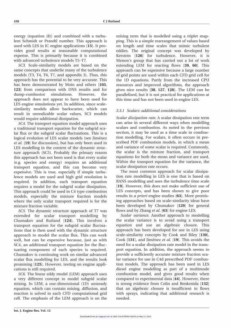
energy (equation (8)) and combined with a turbu-

lent Schmidt or Prandtl number. This approach is

used with LES in IC engine applications [15]. It pro-

vides good results at reasonable computational

expense. This is primarily because it is combined

with advanced turbulence models T5–T7.

SC3. Scale-similarity models are based on the

same concepts that underlie many of the turbulence

models (T3, T4, T6, T7, and appendix 3). Thus, this

approach has the potential to be very accurate. This

has been demonstrated by Moin and others [103,

123] from comparison with DNS results and for

dump-combustor simulations. However, the

approach does not appear to have been used for

LES engine simulations yet. In addition, since scale-

similarity models allow backscatter, which can

result in unrealizable scalar values, SC3 models

would require additional dissipation.

SC4. The transport equation model approach uses

a traditional transport equation for the subgrid sca-

lar flux or the subgrid scalar fluctuations. This is a

logical evolution of LES scalar models (see Jimenez

et al. [19] for discussion), but has only been used in

LES modelling in the context of the dynamic struc-

ture approach (SC5). Probably the primary reason

this approach has not been used is that every scalar

(e.g. species and energy) requires an additional

transport equation, and this can become very

expensive. This is true, especially if simple turbu-

lence models are used and high grid resolution is

required. In addition, each transport equation

requires a model for the subgrid scalar dissipation.

This approach could be used in C4 type combustion

models, especially the mixture fraction models

where the only scalar transport required is for the

mixture fraction variable.

SC5. The dynamic structure approach of T7 was

extended for scalar transport modelling by

Chumakov and Rutland [124]. This involves a

transport equation for the subgrid scalar fluctua-

tions that is then used with the dynamic structure

approach to model the scalar flux. This can work

well, but can be expensive because, just as with

SC4, an additional transport equation for the fluc-

tuating component of each species is required.

Chumakov is continuing work on similar advanced

scalar flux modelling for LES, and the results look

promising [125]. However, testing on engine appli-

cations is still required.

SC6. The linear eddy model (LEM) approach uses

a very different concept to model subgrid scalar

mixing. In LEM, a one-dimensional (1D) unsteady

equation, which can contain mixing, diffusion, and

reaction is solved in each CFD computational grid

cell. The emphasis of the LEM approach is on the

mixing term that is modelled using a triplet map-

ping. This is a simple rearrangement of values based

on length and time scales that mimic turbulent

eddies. The original concept was developed by

Kerstein [126] for turbulence. However, it is

Menon’s group that has carried out a lot of work

extending LEM for reacting flows [39, 60]. This

approach can be expensive because a large number

of grid points are used within each CFD grid cell for

the 1D equations. Partly from the increased CPU

resources and improved algorithms, the approach

gives nice results [38, 127, 128]. The LEM can be

parallelized, but it is not practical for applications at

this time and has not been used in engine LES.

3.3.1 Scalars: additional considerations

Scalar dissipation rate. A scalar dissipation rate term

can arise in several different ways when modelling

scalars and combustion. As noted in the previous

section, it may be used as a time scale in combus-

tion modelling. For scalars, it often occurs in pre-

scribed PDF combustion models, in which a mean

and variance of some scalar is required. Commonly,

the scalar is the mixture fraction, and transport

equations for both the mean and variance are used.

Within the transport equation for the variance, the

scalar dissipation rate occurs.

The most common approach for scalar dissipa-

tion rate modelling in LES is one that is based on

RANS modelling and uses the turbulence time scale

[19]. However, this does not make sufficient use of

LES concepts, and has been shown to give poor

results in a priori engine studies [63]. More promis-

ing approaches based on scale-similarity ideas have

been developed by Chumakov [129] for general

flows and by Zhang et al. [63] for engine LES.

Scalar variance. Another approach to modelling

the scalar variance is to avoid using a transport

equation and use an algebraic closure. This

approach has been developed for use in LES using

scale-similarity concepts by Cook and Riley [130],

Cook [131], and Jimenez et al. [19]. This avoids the

need for a scalar dissipation rate model in the trans-

port equation. In addition, the approach seems to

provide a sufficiently accurate mixture fraction sca-

lar variance for use in C4d prescribed PDF combus-

tion models. The approach has been used in LES

diesel engine modelling as part of a multimode

combustion model, and gives good results when

compared to experimental data [44]. However, there

is strong evidence from Colin and Benkenida [132]

that an algebraic closure is insufficient in flows

with sprays, indicating that additional research is

needed.

438 C J Rutland




3.3.2 Scalar mixing: recommendations

1. Scalar mixing and combustion models are often

linked through terms such as the scalar dissipa-

tion rate. This requires that the scalar models at

least be consistent with the combustion model

being used.

2. One major trend is to include detailed chemistry

effects by direct integration or tabulation meth-

ods. This means that a large number of scalar

transport equations are being solved. Thus, sca-

lar mixing models should be fairly simple to

avoid large computational costs.

3. Scalar mixing models that use a turbulent visc-

osity and mean scalar gradient (SC2) can be suf-

ficient, provided they are coupled with advanced

turbulence models (T5–T7) that provide addi-

tional subgrid variables such as Ksgs.

4. Higher order scalar mixing models that use

transport equations for subgrid quantities (SC4,

SC5) may offer better potential for accuracy but

at a higher computational cost.

3.4 Fuel-spray modelling

Most engine simulations use the Lagrangian spray

parcel methodology originally developed for RANS

approaches in which the CFD grid is not resolved

around spray particles. This approach was initially

developed by O’Rouke and Amsden in the KIVA-II

code, and this still provides the basis of most engine

spray CFD modelling [133]. In this context, the

spray modelling issue is how to represent the sub-

grid interaction of the Lagrangian spray particles

with the continuous gas phase. This interaction

includes momentum transfer (e.g. drag), kinetic

energy transfer, heat and mass transfer during eva-

poration, and models for atomization, breakup, and

collisions. This is an extensive list of complex physi-

cal processes, and they all require modelling. The

range of physical processes and their complexity is

probably why most spray models in LES are exten-

sions of RANS approaches and little work has been

carried out on developing new spray models specifi-

cally for LES applications.

A review of more general spray modelling was

provided by Jiang et al. [134]. They discussed basic

issues of using the parcel approach for RANS and

LES. Most simulations of engines with sprays have

used existing RANS spray models with simple mod-

ifications for use with LES turbulence models. In a

series of papers, Bellan et al. have carried out

extensive work exploring particle-based spray mod-

els for both DNS and LES simulations [135–139].

This is more fundamental work, but the target

applications are those that use the Lagrangian par-

cel approach. Some of their major conclusions are

listed below.

1. A good LES turbulence model is essential

because the spray is affected by both the large-

scale flow features as well as the subgrid effects.

Both require a good turbulence model.

2. Viscosity turbulence models (T2–T6) can work

with spray models, as shown by comparisons

with DNS results. However, in an actual LES

simulation, additional dissipation is needed. In

general, spray models that work well in compari-

son to DNS results often are not sufficient for

use in a stand-alone LES simulation.

3. The subgrid turbulence and scalar mixing mod-

els should consider anisotropy and inhomo-

geneities. This is because the length scale of the

spray parcels is so much smaller than the grid

scale that these differences can be important.

4. The number of parcels that is appropriate for use

in the LES spray models is not well understood.

5. There must be full interaction between the spray

and the gas phase. This means that partial mod-

els that only include gas flow affects on the

spray but ignore spray effects on the gas flow

are not sufficient.

6. The Lagrangian spray parcels are not located at

the grid points. Thus, obtaining accurate values

of the gas phase variables (velocity, temperature,

concentration) at the spray parcel location is

important. A simple interpolation is not suffi-

cient, and Bellan et al. found that a random per-

turbation from a normal distribution is required.

For drag effects, this is similar to including tur-

bulent dispersion effects commonly used in

RANS spray models.

This is a rigorous list to keep in mind as spray mod-

els are developed and evolved for LES engine simu-

lations. A list of the spray modelling approaches

that could be used in engine LES applications

appears in Table 5.

S1. The simplest approach to LES spray models is

to use laminar correlations for subgrid interactions

such as drag and evaporation. This means obtaining

droplet drag, heat transfer, and mass transfer effects

on both the gas and liquid phases through correla-

tions appropriate for laminar flow around drops.

This approach might be acceptable for very high

resolution, scientific LES. However, it is inappropri-

ate for engineering LES since there are subgrid tur-

bulence effects that are important and need to be

modelled.





S2. The use of RANS correlations is probably the

most commonly used approach for spray modelling

in LES. Here, subgrid models based on single dro-

plet turbulent correlations for drag, turbulent dis-

persion, evaporation, and even breakup and

collision are used with LES turbulence models.

Successful examples of this approach for engines

can be found in: (a) Hu et al. [15] and Hu and

Rutland [78] for diesel applications with the T7 tur-

bulence model and a multimode combustion

model, (b) Kaario et al. and Vuorinen et al. at

Helsinki University of Technology [10, 140] for die-

sel applications with T5 and later T1 turbulence

models and a C3a combustion model, and (c) Aria

et al. [141] for direct injection gasoline applications

using a T2 turbulence model.

In a series of papers, a group at Doshisha

University has explored spray models using KIVA

with the T5 turbulence model [52, 53, 142–144].

The spray models were essentially the same as the

RANS-based models available in the original KIVA

code. Their work focused on non-engine simula-

tions of spray bombs with fairly dense grids. They

made nice comparisons with experimental work,

demonstrating that the S2 approach for spray mod-

elling can provide reasonable results with very high

grid resolution. One interesting aspect of their work

was the addition of a higher order numerical

method for momentum equation convection terms.

Their results demonstrated moderate improvement

with the new numerical technique. However, it was

achieved only on a simple Cartesian grid used in

their spray bomb domain and might be difficult to

achieve on a practical engine grid.

S3. The most desirable spray models would be

those that are developed specifically for LES and are

fully consistent with the turbulence and scalar mix-

ing models. These would take advantage of the

information from the LES models such as subgrid

turbulence, ksgs, for modelling the many fuel-spray

processes. There was some initial work on this car-

ried out by Pannala et al. [145]. They made an

important observation that models should consider

that the interaction between the spray and the gas

flow occurs at both the subgrid and the resolved

scales. They developed a partitioning to account for

this but, unfortunately, the work was not well

explained so it is hard to evaluate.

More recently, Bharadwaj et al. developed an LES

specific model for diesel sprays [146, 147]. The

model reformulated the spray source term in the

subgrid kinetic energy transport equation of a T7

turbulence model. The model used a deconvolution

method [148] to obtain a better representation of

subgrid velocities at the droplet location. The model

addressed one of the primary problems with using

RANS spray models with LES turbulence models. In

these situations, it is not uncommon to see high-

speed sprays significantly over-penetrating unless a

very dense grid is used [142]. This can be traced to

the RANS spray source term being modelled only as

a sink of kinetic energy, whereas in the LES formula-

tion, the spray can be either a source or a sink

depending on the spray velocities and the ambient

gas conditions. Figure 5 demonstrates how an LES

simulation without an appropriate source term has

significant over-penetration of the liquid parcels

while the addition of the source term from

Bharadwaj et al. brings the penetration in line with

the experimentally calibrated RANS results.

S4. Recently, there have been a number of publi-

cations describing high-resolution, very detailed

simulations of fuel sprays. In a paper by deVillers

et al. [149], a volume of fluid (VOF) approach was

used to study near-nozzle flow and primary breakup

in a diesel spray. They used the OpenFOAM code

[150, 151] with a T5 turbulence model on a very

dense grid. The VOF method used was adapted for

droplet breakup, but no other specific LES spray

models were used. In later work, Befrui et al. [152]

used the VOF method to simulate internal and

near-nozzle flow for gasoline direct injection appli-

cations. They used the OpenFOAM code with a T5

turbulence model, a very dense grid and no special

Table 5 Classification of LES spray modelling approaches

Model type Advantages Disadvantages

S1 Laminar correlations Simple, well-established submodels Ignores important physical processesfrom subgrid turbulence

S2 RANS correlations Uses established turbulence models Does not consider specific advantagesof LES formulations

S3 LES modifications Integrates spray models into LESmethodology

Still early in development phase; littleexperimental or DNS data forvalidation

S4 Continuous phase, non-particle models More authentic representation thanLagrangian parcel approaches

Computational very expensive and notapplicable to full combustionchamber simulations

440 C J Rutland




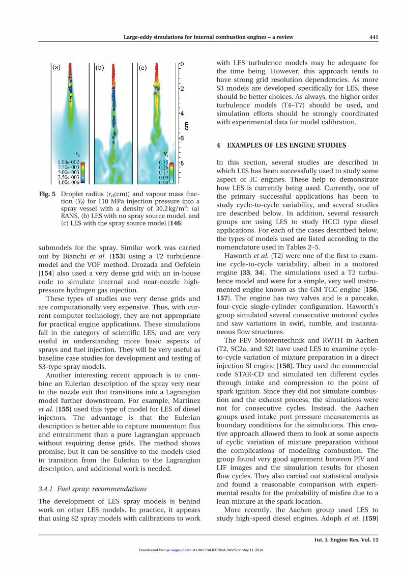
submodels for the spray. Similar work was carried

out by Bianchi et al. [153] using a T2 turbulence

model and the VOF method. Drozada and Oefelein

[154] also used a very dense grid with an in-house

code to simulate internal and near-nozzle high-

pressure hydrogen gas injection.

These types of studies use very dense grids and

are computationally very expensive. Thus, with cur-

rent computer technology, they are not appropriate

for practical engine applications. These simulations

fall in the category of scientific LES, and are very

useful in understanding more basic aspects of

sprays and fuel injection. They will be very useful as

baseline case studies for development and testing of

S3-type spray models.

Another interesting recent approach is to com-

bine an Eulerian description of the spray very near

to the nozzle exit that transitions into a Lagrangian

model further downstream. For example, Martinez

et al. [155] used this type of model for LES of diesel

injectors. The advantage is that the Eulerian

description is better able to capture momentum flux

and entrainment than a pure Lagrangian approach

without requiring dense grids. The method shows

promise, but it can be sensitive to the models used

to transition from the Eulerian to the Lagrangian

description, and additional work is needed.

3.4.1 Fuel spray: recommendations

The development of LES spray models is behind

work on other LES models. In practice, it appears

that using S2 spray models with calibrations to work

with LES turbulence models may be adequate for

the time being. However, this approach tends to

have strong grid resolution dependencies. As more

S3 models are developed specifically for LES, these

should be better choices. As always, the higher order

turbulence models (T4–T7) should be used, and

simulation efforts should be strongly coordinated

with experimental data for model calibration.

4 EXAMPLES OF LES ENGINE STUDIES

In this section, several studies are described in

which LES has been successfully used to study some

aspect of IC engines. These help to demonstrate

how LES is currently being used. Currently, one of

the primary successful applications has been to

study cycle-to-cycle variability, and several studies

are described below. In addition, several research

groups are using LES to study HCCI type diesel

applications. For each of the cases described below,

the types of models used are listed according to the

nomenclature used in Tables 2–5.

Haworth et al. (T2) were one of the first to exam-

ine cycle-to-cycle variability, albeit in a motored

engine [33, 34]. The simulations used a T2 turbu-

lence model and were for a simple, very well instru-

mented engine known as the GM TCC engine [156,

157]. The engine has two valves and is a pancake,

four-cycle single-cylinder configuration. Haworth’s

group simulated several consecutive motored cycles

and saw variations in swirl, tumble, and instanta-

neous flow structures.

The FEV Motorentechnik and RWTH in Aachen

(T2, SC2a, and S2) have used LES to examine cycle-

to-cycle variation of mixture preparation in a direct

injection SI engine [158]. They used the commercial

code STAR-CD and simulated ten different cycles

through intake and compression to the point of

spark ignition. Since they did not simulate combus-

tion and the exhaust process, the simulations were

not for consecutive cycles. Instead, the Aachen

groups used intake port pressure measurements as

boundary conditions for the simulations. This crea-

tive approach allowed them to look at some aspects

of cyclic variation of mixture preparation without

the complications of modelling combustion. The

group found very good agreement between PIV and

LIF images and the simulation results for chosen

flow cycles. They also carried out statistical analysis

and found a reasonable comparison with experi-

mental results for the probability of misfire due to a

lean mixture at the spark location.

More recently, the Aachen group used LES to

study high-speed diesel engines. Adoph et al. [159]

Fig. 5 Droplet radius (rd(cm)) and vapour mass frac-tion (Yf) for 110 MPa injection pressure into aspray vessel with a density of 30.2 kg/m3: (a)RANS, (b) LES with no spray source model, and(c) LES with the spray source model [146]





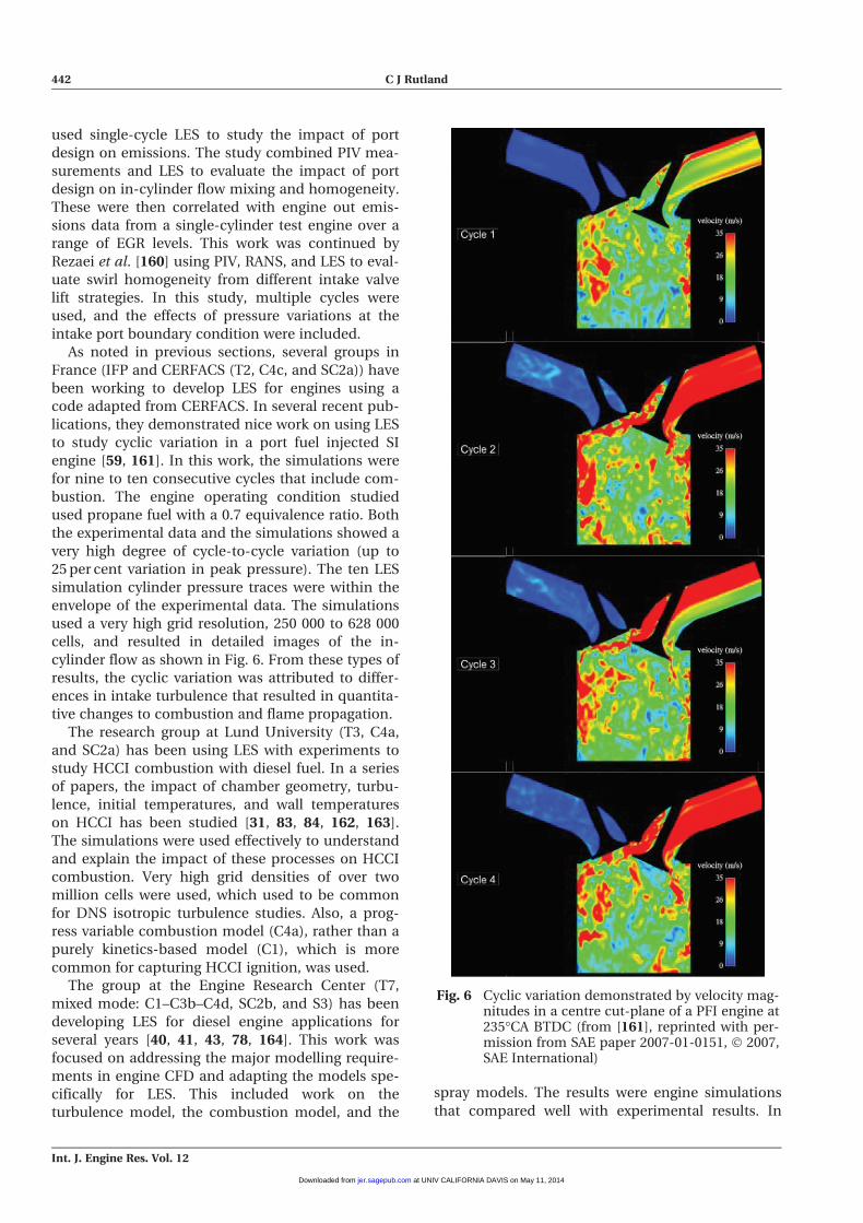
used single-cycle LES to study the impact of port

design on emissions. The study combined PIV mea-

surements and LES to evaluate the impact of port

design on in-cylinder flow mixing and homogeneity.

These were then correlated with engine out emis-

sions data from a single-cylinder test engine over a

range of EGR levels. This work was continued by

Rezaei et al. [160] using PIV, RANS, and LES to eval-

uate swirl homogeneity from different intake valve

lift strategies. In this study, multiple cycles were

used, and the effects of pressure variations at the

intake port boundary condition were included.

As noted in previous sections, several groups in

France (IFP and CERFACS (T2, C4c, and SC2a)) have

been working to develop LES for engines using a

code adapted from CERFACS. In several recent pub-

lications, they demonstrated nice work on using LES

to study cyclic variation in a port fuel injected SI

engine [59, 161]. In this work, the simulations were

for nine to ten consecutive cycles that include com-

bustion. The engine operating condition studied

used propane fuel with a 0.7 equivalence ratio. Both

the experimental data and the simulations showed a

very high degree of cycle-to-cycle variation (up to

25 per cent variation in peak pressure). The ten LES

simulation cylinder pressure traces were within the

envelope of the experimental data. The simulations

used a very high grid resolution, 250 000 to 628 000

cells, and resulted in detailed images of the in-

cylinder flow as shown in Fig. 6. From these types of

results, the cyclic variation was attributed to differ-

ences in intake turbulence that resulted in quantita-

tive changes to combustion and flame propagation.

The research group at Lund University (T3, C4a,

and SC2a) has been using LES with experiments to

study HCCI combustion with diesel fuel. In a series

of papers, the impact of chamber geometry, turbu-

lence, initial temperatures, and wall temperatures

on HCCI has been studied [31, 83, 84, 162, 163].

The simulations were used effectively to understand

and explain the impact of these processes on HCCI

combustion. Very high grid densities of over two

million cells were used, which used to be common

for DNS isotropic turbulence studies. Also, a prog-

ress variable combustion model (C4a), rather than a

purely kinetics-based model (C1), which is more

common for capturing HCCI ignition, was used.

The group at the Engine Research Center (T7,

mixed mode: C1–C3b–C4d, SC2b, and S3) has been

developing LES for diesel engine applications for

several years [40, 41, 43, 78, 164]. This work was

focused on addressing the major modelling require-

ments in engine CFD and adapting the models spe-

cifically for LES. This included work on the

turbulence model, the combustion model, and the

spray models. The results were engine simulations

that compared well with experimental results. In

Fig. 6 Cyclic variation demonstrated by velocity mag-nitudes in a centre cut-plane of a PFI engine at235�CA BTDC (from [161], reprinted with per-mission from SAE paper 2007-01-0151, � 2007,SAE International)

442 C J Rutland




addition, when applied to HCCI combustion, the

simulation results were able to capture cyclic varia-

bility due to temperature non-homogeneities in the

spray region.

5 PROSPECTS FOR THE FUTURE

The outlook for using LES in IC engine modelling is

very good. The primary engine submodels, as out-

lined in this review, are maturing. User experience

is growing, and the number of high-quality studies

using LES is rapidly increasing.

There is still a need for model improvements,

especially in the areas of combustion and sprays.

However, this need is not unique to LES. In addi-

tion, improvements and adaptation to LES are

needed for many second-tier models such as wall

heat transfer, nozzle flows for spray boundary con-

ditions, spray breakup, and atomization.

Improvements to numerical methods are also

needed. However, improvements will be somewhat

limited by the complexity of the domain, moving

boundaries, and numerical treatment of fuel sprays.

These limitations should not preclude the use of

LES in engines, as there is still much to be gained in

terms of increasing the types of problems that can

be studied.

Important issues that remain on the horizon are

validation and establishing ‘best practices’ for LES

engine simulations. Increasing activity and publica-

tions will help to address these issues naturally. In

addition, there is a high probability that research

groups are already establishing programs to address

these issues as the potential of LES becomes clearer.

Thus, users are encouraged to apply LES to

appropriate problems that are enhanced or require

the increased sensitivity to flow unsteadiness and

large-scale structures. For example, topics such as

cyclic variation and design sensitivity are probably

best studied with LES. However, users should be

aware of the large range of models used in engine

CFD and carefully choose the appropriate LES capa-

ble submodels. The taxonomy presented in this

review should be helpful in this regard.

FUNDING

The author acknowledges support over the years in

the broad area of LES for engineering applica-

tions from a number of sources, including the

US Department of Energy [grant numbers DE-FC04-

02AL67612, DE-FC26-06NT42628, and DE-EE000

0202], General Motors Research primarily through

the GM-UW Cooperative Research Lab, Caterpillar

Inc., the National Science Foundation [grant num-

ber 0500056], and the Air Force Office of Scientific

Research [grant number F49620-02-1-0348].

� Authors 2011

REFERENCES

1 Niatoh, K., Ito, H., and Takagi, Y. Large eddysimulation of premixed-flame in engine based onthe multi-level formulation and the renormaliza-tion group theory. SAE paper 920590, 1992.

2 Ferziger, J. H. Simulation of complex turbulentflows: recent advances and prospects in wind engi-neering. J. Wind Eng. Ind. Aerodyn., 1993, 46–47,195–212.

3 Fureby, C., Tabor, G., Weller, H. G., and Gos-man, A. D. A comparative study of subgrid scalemodels in homogeneous isotropic turbulence.Phys. Fluids, 1997, 9(5), 1416–1429.

4 Fureby, C. Towards the use of large eddy simula-tion in engineering. Prog. Aerosp. Sci., 2008, 44(6),381–396.

5 Geurts, B. J. Modern simulation strategies for tur-bulent flow, 2001 (Edwards, Philadelphia, PA).

6 Piomelli, U. Large-eddy simulation: achieve-ments and challenges. Prog. Aerosp. Sci., 1999, 35,335–362.

7 Pope, S. B. Ten questions concerning the large-eddy simulation of turbulent flows. New J. Phys.,1999, 6(35), 1–24.

8 Poinsot, T. and Veynante, D. Theoretical andnumerical combustion, 2005 (Edwards, Philadel-phia, PA).

9 Pope, S. B. Turbulent flows, 2000 (Cambridge Uni-versity Press, Cambridge, UK).

10 Kaario, O., Pokela, H., Kjaldman, L., Tiainen, J.,and Larmi, M. LES and RNG turbulence modelingin DI diesel engines. SAE paper 2003-01-1069, 2003.

11 Germano, M., Piomelli, U., Moin, P., andCabot, W. H. A dynamic subgrid-scale eddy viscos-ity model. Phys. Fluids A: Fluid Dyn., 1991, 3(7),1760–1765.

12 Lu, H., Rutland, C. J., and Smith, L. M. A prioritest of one-equation LES modeling of rotating tur-bulence. J. Turb., 2007, 8(37), pp. 127, DOI:10.1080/14685240701493947.

13 Ferziger, J. H. Simulation of incompressible turbu-lent flows. J. Comput. Phys., 1987, 69(1), 1–48.

14 Clark, R. A., Ferziger, J. H., and Reynolds, W. C.Evaluations of subgrid-scale models using an accu-rately simulated turbulent flow. J. Fluid Mech.,1979, 91, 1–16.

15 Hu, B., Jhavar, R., Singh, S., Reitz, R. D., andRutland, C. J. Combustion modeling of diesel com-bustion with partially premixed conditions. SAEpaper 2007-01-0163, 2007.

16 Pitsch, H. Large-eddy simulation of turbulentcombustion. Ann. Rev. Fluid Mech., 2006, 38(1),453–482.





17 Kempf, A., Flemming, F., Janicka, J., Bellan, J.,Gore, J. P., and Ihme, M. Investigation of lengths-cales, scalar dissipation, and flame orientation in apiloted diffusion flame by LES, Proceedings of theCombustion Institute, 2005, 30, pp. 557–565.

18 Smagorinsky, J. General circulation experimentswith the primitive equations. Mon. Weather Rev.,1963, 91(3), 99–164.

19 Jimeenez, C., Ducros, F., Cuenot, B., and Bee-dat, B. Subgrid scale variance and dissipation of ascalar field in large eddy simulations. Phys. Fluids,2001, 13(6), 1748.

20 Boris, J. P., Grinstein, F. F., Oran, E. S., andKolbe, R. L. New insights into large eddy simula-tion. Fluid Dyn. Res., 1992, 10(4–6), 199–228.

21 Celik, I., Yavuz, I., Smirnov, A., Smith, J.,Amin, E., and Gel, A. Prediction of in-cylinder tur-bulence for IC engines. Combust. Sci. Technol.,2000, 153(1), 339–368.

22 Amsden, A. KIVA-3V: a block-structure KIVA pro-gram for engines with vertical or canted valves.Los Alamos Report LA-13313-MS, (T3 Group inter-nal report, approved for public release), 1997.

23 Celik, I., Yavuz, I., and Smirnov, A. Large eddysimulations of in-cylinder turbulence for internalcombustion engines: a review. Int. J. Engine Res.,2001, 2(2), 119–148.

24 Nicoud, F. and Ducros, F. Subgrid-scale stressmodelling based on the square of the velocity gra-dient tensor. Flow, Turbul. Combust., 1999, 62,183–200.

25 Moureau, V., Barton, I., Angelberger, C., andPoinsot, T. Towards large eddy simulation in inter-nal-combustion engines: simulation of a com-pressed tumble flow. SAE paper 2004-01-1995, 2004.

26 Devesa, A., Moreau, J., Poinsot, T., and Helie, J.Large eddy simulations of jet / tumble interactionin a GDI model engine flow. SAE paper 2004-01-1997, 2004.

27 Frusiani, F., Forte, C., and Bianchi, G. M. Assess-ment of a numerical methodology for large eddysimulation of ice wall bounded non-reactive flows.SAE paper 2007-01-4145, 2007.

28 Brusiani, F. and Bianchi, G. M. LES simulation ofICE non-reactive flows in fixed grids. SAE paper2008-01-0959, 2008.

29 Bardina, J., Ferziger, J. H., and Reynolds, W. C.Improved subgrid-scale models for large eddysimulation. AIAA paper AIAA 1980-1357, 1980.

30 Meneveau, C. and Katz, J. Scale-invariance andturbulence models for large-eddy simulation. Ann.Rev. Fluid Mech., 2000, 32(1), 1–32.

31 Yu, R., Bai, X. S., Hildingsson, L., Hultqvist, A.,and Miles, P. Numerical and experimental investi-gation of turbulent flows in a diesel engine. SAEpaper 2006-01-3436, 2006.

32 Meneveau, C., Lund, T. S., and Cabot, W. H. ALagrangian dynamic subgrid-scale model of turbu-lence. J. Fluid Mech., 1996, 319, 353–385.

33 Haworth, D. C. Large-eddy simulation of in-cylinder flows. Oil Gas Sci. Technol., 1999, 54(2),175–185.

34 Haworth, D. C. and Jansen, K. Large-eddy simula-tion on unstructured deforming meshes: towardsreciprocating IC engines. Comput. Fluids, 2000,29(5), 493–524.

35 Yoshizawa, A. and Horiuti, K. A statistically-derivedsubgrid-scale kinetic energy model for the large-eddy simulation of turbulent flows. J. Phys. Soc.Japan, 1985, 54(8), 2834–2839.

36 Kim, W. -W. and Menon, S. A new dynamic one-equation subgrid scale model for large-eddy simu-lations. AIAA paper 95-0356, 1995.

37 Nelson, C. and Menon, S. Unsteady simulations ofcompressible spatial mixing layers. AIAA paperAIAA 98-0786, 1998.

38 Kim, W.- W., Menon, S., and Mongia, H. C. Large-eddy simulation of a gas turbine combustor flow.Combust. Sci. Technol., 1999, 143(1), 25–62.

39 Sone, K. and Menon, S. Effect of subgrid modelingon the in-cylinder unsteady mixing process in adirect injection engine. J. Eng. Gas Turbine Power,2003, 125(2), 435.

40 Pomraning, E. and Rutland, C. J. Dynamic one-equation nonviscosity large-eddy simulationmodel. AIAA J., 2002, 40(4), 689–701.

41 Chumakov, S. G. and Rutland, C. J. Dynamicstructure subgrid-scale models for large eddy simu-lation. Int. J. Numer. Methods Fluids, 2005, 47(8–9),911–923.

42 Lu, H., Rutland, C. J., and Smith, L. M. A posterioritests of one-equation LES modeling of rotatingturbulence. Int. J. Mod. Phys. C, 2008, 19(12),1949–1964.

43 Jhavar, R. and Rutland, C. J. Using large eddysimulations to study mixing effects in early injec-tion diesel engine combustion. SAE paper 2006-01-0871, 2006.

44 Banerjee, S., Liang, T., Rutland, C. J., and Hu, B.Validation of an LES multi mode combustionmodel for diesel combustion. SAE paper 2010-01-0361, 2010.

45 Kannepalli, C. and Piomelli, U. Large-eddy simu-lation of a three-dimensional shear-driven tur-bulent boundary layer. J. Fluid Mech., 2000, 423,175–203.

46 Chang III, P. A., Piomelli, U., and Blake, W. K.Relationship between wall pressure and velocity-field sources. Phys. Fluids, 1999, 11(11), 3434–3448.

47 Cabot, W. and Moin, P. Approximate wall bound-ary conditions in the large-eddy simulation of highReynolds number flow. Flow, Turbul. Combust.,2000, 63(1), 269–291.

48 Piomelli, U. Wall-layer models for large-eddysimulations. Prog. Aerosp. Sci., 2008, 44(6), 437–446.

49 Frohlich, J. and von Terzi, D. Hybrid LES/RANSmethods for the simulation of turbulent flows.Prog. Aerosp. Sci., 2008, 44(5), 349–377.

50 Rodi, W., Ferziger, J. H., Breuer, M., and Pour-quie, M. Status of large eddy simulation: results ofa workshop. J. Fluids Eng., Trans. ASME, 1997,119(2), 248–262.

444 C J Rutland




51 Ghosal, S. and Moin, P. The basic equations forthe large eddy simulation of turbulent flowsin complex geometry. J. Comput. Phys., 1995, 118,24–37.

52 Hori, T., Kuge, T., Senda, J., and Fujimoto, H.Large eddy simulation of diesel spray combustionwith eddy-dissipation model and CIP method byuse of KIVALES. SAE paper 2007-01-0247, 2007.

53 Hori, T., Kuge, T., Senda, J., and Fujimoto, H.Effect of convective schemes on LES of fuel sprayby use of KIVALES. SAE paper 2008-01-0930, 2008.

54 Thobois, L., Rymer, G., Souleres, T., andPoinsot, T. Large-eddy simulation in IC enginegeometries. SAE paper 2004-01-1854, 2004.

55 Thobois, L., Lauvergne, R., and Poinsot, T. UsingLES to investigate reacting flow physics in enginedesign process. SAE paper 2007-01-0166, 2007.

56 Reitz, R. D. and Rutland, C. J. Development andtesting of diesel engine CFD models. Prog. EnergyCombust. Sci., 1995, 21(2), 173–196.

57 Liang, L., Reitz, R. D., Iyer, C. O., and Yi, J. Mod-eling knock in spark-ignition engines using a G-equation combustion model incorporatingdetailed chemical kinetics. SAE paper 2007-01-0165, 2007.

58 Attard, W. P., Toulson, E., Watson, H., andHamori, F. Abnormal combustion including megaknock in a 60% downsized highly turbocharged PFIengine. SAE paper 2010-01-1456, 2010.

59 Vermorel, O., Richard, S., Colin, O., Angelber-ger, C., Benkenida, A., and Veynante, D. Towardsthe understanding of cyclic variability in a sparkignited engine using multi-cycle LES. Combust.Flame, 2009, 156(8), 1525–1541.

60 Menon, S. Subgrid combustion modelling forlarge-eddy simulations. Int. J. Engine Res., 2000,1(2), 209–227.

61 Veynante, D. and Vervisch, L. Turbulent combus-tion modelling. Prog. Energy Combust. Sci., 2002,28(3), 193–266.

62 Hilbert, R., Tap, F., El-Rabii, H., andThevenin, D. Impact of detailed chemistry andtransport models on turbulent combustion simu-lations. Prog. Energy Combust. Sci., 2004, 30(1),61–117.

63 Zhang, Y., Ghandhi, J. B., Petersen, B., andRutland, C. J. Large eddy simulation of scalar dissi-pation rate in an internal combustion engine. SAEpaper 2010-01-0625, 2010.

64 Kong, S.-C. and Reitz, R. D. Use of detailedchemical kinetics to study HCCI engine combus-tion with consideration of turbulent mixingeffects. J. Eng. Gas Turbines Power, 2002, 124(3),702–707.

65 Yang, S. and Reitz, R. D. Integration of a continu-ous multi-component fuel evaporation model withan improved G-equation combustion and detailedchemical kinetics model with application to GDIengines. SAE paper 2009-01-0722, 2009.

66 Kokjohn, S., Hanson, R. M., Splitter, D. A., andReitz, R. D. Experiments and modeling of dual-fuel

HCCI and PCCI combustion using in-cylinder fuelblending. SAE paper 2009-01-2647, 2009.

67 Shi, Y., Kokjohn, S., Ge, H., and Reitz, R. D. Effi-cient multidimensional simulation of HCCI and DIengine combustion with detailed chemistry. SAEpaper 2009-01-0701, 2009.

68 Liang, L., Naik, C. V., Puduppakkam, K., Wang, C.,Modak, A., Meeks, E., Ge, H., Reitz, R. D., andRutland, C. J. Efficient simulation of diesel enginecombustion using realistic chemical kinetics in CFD.SAE paper 2010-01-0178, 2010.

69 Galpin, J., Angelberger, C., Naudin, A., andVervisch, L. Large-eddy simulation of H 2–air auto-ignition using tabulated detailed chemistry. J. Tur-bul., 2008, 9(13), 1–21.

70 Fiorina, B., Vicquelin, R., Auzillon, P.,Darabiha, N., Gicquel, O., and Veynante, D. A fil-tered tabulated chemistry model for LES of pre-mixed combustion. Combust. Flame, 2010, 157(3),465–475.

71 Barths, H., Antoni, C., and Peters, N. Three-dimensional simulation of pollutant formation in aDI diesel engine using multiple interactive flame-lets. SAE paper 982459, 1998.

72 Hergart, C., Barths, H., and Peters, N. Modelingthe combustion in a small-bore diesel engine usinga method based on representative interactive fla-melets. SAE paper 1999-01-3550, 1999.

73 Hasse, C., Barths, H., and Peters, N. Modelling theeffect of split injections in diesel engines using rep-resentative interactive flamelets. SAE paper 1999-01-3547, 1999.

74 Felsch, C., Luckhchoura, V., Weber, J.Peters, N., Hasse, C., Wiese, W., Pischinger, S.,Kolbeck, A., and Adomeit, P. Applying represen-tative interactive flamelets (rif) with specialemphasis on pollutant formation to simulate a DIdiesel engine with roof-shaped combustion cham-ber and tumble charge motion. SAE paper 2007-01-0167, 2007.

75 Abraham, J., Bracco, F. V., and Reitz, R. D. Com-parison of computed and measured premixedcharged engine combustion. Combust. Flame,1985, 60(3), 309–322.

76 Kong, S. -C. and Reitz, R. D. Multidimensionalmodeling of diesel ignition and combustion usinga multistep kinetics models. J. Eng. Gas TurbinesPower, 1993, 115(4), 781–789.

77 Rao, S. and Rutland, C. J. A flamelet time scalemodel for non-premixed combustion includingchemical kinetic effects. Combust. Flame, 2003,133(1–2), 189–191.

78 Hu, B. and Rutland, C. J. Flamelet modeling withLES for diesel engine simulations. SAE paper 2006-01-0058, 2006.

79 Bray, K. N. C. Interaction between turbulence andcombustion. In 17th International Symposiumon Combustion, 1979, pp. 223–233 (CombustionInstitute).

80 Kerstein, A., Ashurst, W., and Williams, F. Fieldequation for interface propagation in an unsteady





homogeneous flow field. Phys. Rev. A, 1988, 37(7),2728–2731.

81 Zimont, V. L. Correlation between two approachesto combustion modeling based on the progressvariable the scalar G. In 29th International Sympo-sium on Combustion, 2001, vol. 29 (CombustionInstitute).

82 Zimont, V. L., Polifke, W., Bettelini, M., andWeisenstein, W. An efficient computational modelfor premixed turbulent combustion at high Rey-nolds numbers based on a turbulent flame speedclosure. J. Eng. Gas Turbines Power, 1998, 120(3),526–532.

83 Yu, R., Bai, X. S., Vressner, A., Hultqvist, A.,Johansson, B., Olofsson, J., Seyfried, H.,Sjoholm, J., Richter, M., and Alden, M. Effect ofturbulence on HCCI combustion. SAE paper 2007-01-0183, 2007.

84 Joelsson, T., Yu, R., Bai, X. S., Vressner, A., andJohansson, B. Large eddy simulation and experi-ments of the auto-ignition process of lean ethanol/air mixture in HCCI engines. SAE paper 2008-01-1668, 2008.

85 Vressner, A., Egnell, R., and Johansson, B. com-bustion chamber geometry effects on the perfor-mance of an ethanol fueled HCCI engine. SAEpaper 2008-01-1656, 2008.

86 Colin, O., Ducros, F., Veynante, D., and Poin-sot, T. A thickened flame model for large eddysimulations of turbulent premixed combustion.Phys. Fluids, 2000, 12(7), 1843–1863.

87 Peters, N. Turbulent combustion, 2000 (CambridgeUniversity Press, Cambridge, UK).

88 Im, H. G., Lund, T. S., and Ferziger, J. H. Largeeddy simulation of turbulent front propagationwith dynamic subgrid models. Phys. Fluids, 1997,9(12), 3826–3833.

89 Marble, F. E. and Broadwell, J. E. The coherentflame model for turbulent chemical reactions. Proj-ect Squid Report, TRW-9-PU, 1977.

90 Candel, S. M. and Poinsot, T. Flame stretch andthe balance equation for the flame area. Combust.Sci. Technol., 1990, 70, 1–15.

91 Ducros, F., Veynante, D., and Poinsot, T. A com-parison of flamelet models for premixed turbulentcombustion. Combust. Flame, 1993, 95, 101–117.

92 Angelberger, C., Poinsot, T., and Delhay, B.Improving near-wall combustion and wall heattransfer modeling in SI engine computations. SAEpaper 972881, 1997.

93 Henriot, S., Chaouche, A., Cheve, E., andDuclos, J. M. CFD aided development of a Si-Diengine. Oil Gas Sci. Technol., 1999, 54(2), 279–286.

94 Colin, O., Benkenida, A., and Angelberger, C. 3dmodeling of mixing, ignition and combustion phe-nomena in highly stratified gasoline engines. OilGas Sci. Technol., 2003, 58(1), 47–62.

95 Colin, O. and Benkenida, A. The 3-zones extendedcoherent flame model (Ecfm3z) for computing pre-mixed/diffusion combustion. Oil Gas Sci. Technol.,2004, 59(6), 593–609.

96 Subramanian, G., Vervisch, L., and Ravet, F. Newdevelopments in turbulent combustion modellingfor engine design: ECFM-CLEH combustion sub-model. SAE paper 2007-01-0154, 2007.

97 Shi, X., Li, G., and Zheng, Y. DI diesel engine com-bustion modeling based on ECFM-3Z model. SAEpaper 2007-01-4138, 2007.

98 CD-Adapco. STAR-CD, Version 3.26, User manual,2006

99 Weller, H. G., Tabor, G., Gosman, A. D., andFureby, C. Application of a flame-wrinkling LEScombustion model to a turbulent mixing layer. InSymposium (International) on Combustion, 1998,27(1), pp. 899–907.

100 Musculus, M. and Rutland, C. J. Coherent flame-let modeling of diesel engine combustion. Com-bust. Sci. Technol., 1995, 104, 295–337.

101 Richard, S., Colin, O., Vermorel, O., Ben-kenida, A., Angelberger, C., and Veynante, D.Towards large eddy simulation of combustion inspark ignition engines. In Proceedings of the Com-bustion Institute, 2007, vol. 31(2), pp. 3059–3066.

102 Cook, A. W., Riley, J. J., and Kosaly, G. A laminarflamelet approach to subgrid-scale chemistry inturbulent flows. Combust. Flame, 1997, 109(3),332–341.

103 Pierce, C. D. and Moin, P. A dynamic model forsubgrid-scale variance and dissipation rate of aconserved scalar. Phys. Fluids, 10(12), 3041–3044.

104 DesJardin, P. E. and Frankel, S. H. Large eddysimulation of a nonpremixed reacting jet: applica-tion and assessment of subgrid-scale combustionmodels. Phys. Fluids, 1998, 10(9), 2298–2314.

105 Pitsch, H. and Steiner, H. Large-eddy simulationof a turbulent piloted methane/air diffusionflame (Sandia flame D). Phys. Fluids, 2000, 12(10),2541–2554.

106 Galpin, J., Naudin, A., Vervisch, L., Angel-berger, C., Colin, O., and Domingo, P. Large-eddy simulation of a fuel-lean premixed turbulentswirl-burner. Combust. Flame, 2008, 155(1–2),247–266.

107 Lee, D., Pomraning, E., and Rutland, C. J. LESmodeling of diesel engines. SAE paper 2002-01-2779, 1995.

108 Li, Y. H. and Kong, S. -C. Diesel combustionmodelling using LES turbulence model withdetailed chemistry. Combust. Theory Model., 2008,12(2), 205–219.

109 Klimenko, A. Y. Multicomponent diffusion of var-ious admixtures in turbulent flow. Fluid Dyn.,1990, 25, 327–334.

110 Bilger, R. W. Conditional moment closure for tur-bulent reacting flow. Phys. Fluids A, 1993, 5(2),436–444.

111 Wright, Y., Depaola, G., Boulouchos, K., andMastorakos, E. Simulations of spray autoignitionand flame establishment with two-dimensionalCMC. Combust. Flame, 2005, 143(4), 402–419.

112 Kim, S. H., Hu, K. Y., and Fraser, R. A. Numericalprediction of the autoignition delay in a diesel-

446 C J Rutland




like environment by the conditional moment clo-sure model. SAE paper 2000-01-0200, 2000.

113 De Paola, G., Mastorakos, E., Wright, Y. M., andBoulouchos, K. Diesel engine simulations withmulti-dimensional conditional moment closure.Combust. Sci. Technol., 2008, 180(5), 883–899.

114 Steiner, H. and Bushe, W. K. Large eddy simula-tion of a turbulent reacting jet with conditionalsource-term estimation. Phys. Fluids, 2001, 13(3),754–769.

115 Triantafyllidis, A. and Mastorakos, E. Implemen-tation issues of the conditional moment closuremodel in large eddy simulations. Flow, Turbul.Combust., 2010, 84(3), 481–512.

116 Pope, S. B. PDF methods for turbulent reactiveflows. Prog. Energy Combust. Sci., 1985, 11(2),119–192.

117 Haworth, D. C. Progress in probability densityfunction methods for turbulent reacting flows.Prog. Energy Combust. Sci., 2010, 36(2), 168–259.

118 Subramaniam, S. and Haworth, D. C. A probabil-ity density function method for turbulent mixingand combustion on three dimensional unstruc-tured deforming grids. Int. J. Engine Res., 2000,1(2), 171–190.

119 Kung, E. and Haworth, D. C. Transported prob-ability density function (tPDF) modeling fordirect-injection internal combustion engines. SAEpaper 2008-01-0969, 2008.

120 Ihme, M. and Pitsch, H. Prediction of extinctionand reignition in nonpremixed turbulent flamesusing a flamelet/progress variable model 2. Appli-cation in LES of Sandia flames D and E. Combust.Flame, 2008, 155(1–2), 90–107.

121 Tamagna, D., Ra, Y., and Reitz, R. D. Multidi-mensional simulation of PCCI combustion usinggasoline and dual-fuel direct injection withdetailed chemical kinetics. SAE paper 2007-01-0190, 2007.

122 Tamagna, D., Gentili, R., Ra, Y., and Reitz, R. D.Multidimensional simulation of the influence offuel mixture composition and injection timing ingasoline-diesel dual-fuel applications. SAE paper2008-01-0031, 2008.

123 Moin, P., Squires, K. D., Cabot, W. H., andLee, S. A dynamic subgrid-scale model for com-pressible turbulence and scalar transport. Phys.Fluids A, 1991, 3(11), 2746–2757.

124 Chumakov, S. G. and Rutland, C. J. Dynamicstructure models for scalar flux and dissipationin large eddy simulation. AIAA J., 2004, 42(6),1132–1139.

125 Chumakov, S. G. A priori study of subgrid-scaleflux of a passive scalar in isotropic homogeneousturbulence. Phys. Rev. E, 2008, 78(3), 1–11.

126 Kerstein, A. Linear-eddy modelling of turbulenttransport. Part 3. Mixing and differential molecu-lar diffusion in round jets. J. Fluid Mech., 1990,216, 411–435.

127 Goldin, G. M. and Menon, S. A scalar pdf con-struction model for turbulent non-premixed

combustion. Combust. Sci. Technol., 1997, 125(1–6), 47–72.

128 Sen, B. A. and Menon, S. Linear eddy mixingbased tabulation and artificial neural networks forlarge eddy simulations of turbulent flames. Com-bust. Flame, 2010, 157(1), 62–74.

129 Chumakov, S. G. Scaling properties of subgrid-scale energy dissipation. Phys. Fluids, 2007, 19(5),058104.

130 Cook, A. W. and Riley, J. J. A subgrid model forequilibrium chemistry in turbulent flows. Phys.Fluids, 1994, 6(8), 2868–2870.

131 Cook, A. W. Determination of the constant coeffi-cient in scale similarity models of turbulence.Phys. Fluids, 1997, 9(5), 1485–1487.

132 Colin, O. and Benkenida, A. A new scalar fluctua-tion model to predict mixing in evaporatingtwo-phase flows. Combust. Flame, 2003, 134(3),207–227.

133 Amsden, A. KIVA-II: a computer program for che-mically reactive flows with sprays. Los AlamosReport LA-11560-MS (T3 Group internal report,approved for public release), 1989.

134 Jiang, X., Siamas, G. A., Jagus, K., andKarayiannis, T. G. Physical modelling andadvanced simulations of gas–liquid two-phase jetflows in atomization and sprays. Prog. EnergyCombust. Sci., 2010, 36(2), 131–167.

135 Bellan, J. Perspectives on large eddy simulationsfor sprays: issues and solutions. AtomizationSprays, 2000, 10(3–5), 409–425.

136 Miller, R. S. and Bellan, J. Direct numerical simu-lation and subgrid analysis of a transitional dro-plet laden mixing layer. Phys. Fluids, 2000, 12(3),650–671.

137 Okongo, N. A. and Bellan, J. A priori subgridanalysis of temporal mixing layers with evaporat-ing droplets. Phys. Fluids, 2000, 12(6), 1573–1591.

138 Okongo, N. A. and Bellan, J. Consistent large-eddy simulation of a temporal mixing layer ladenwith evaporating drops. Part 1. Direct numericalsimulation, formulation and a priori analysis. J.Fluid Mech., 2004, 499, 1–47.

139 Okongo, N. A., Leboissetier, A., and Bellan, J.Detailed characteristics of drop-laden mixinglayers: large eddy simulation predictions com-pared to direct numerical simulation. Phys. Fluids,2008, 20, 3479–3493.

140 Vuorinen, V., Larmi, M., and Fuchs, L. Large-eddy simulation on the effect of droplet size dis-tribution on mixing of passive scalar in a spray.SAE paper 2008-01-0933, 2008.

141 Arai, J., Oshima, N., Oshima, M., Ito, H., andKubota, M. Large eddy simulation of spray injec-tion to turbulent flows from a slit nozzle. SAEpaper 2007-01-1403, 2007.

142 Hori, T., Senda, J., Kuge, T., and Fujimoto, H. G.Large eddy simulation of non-evaporative andevaporative diesel spray in constant volume vesselby use of KIVALES. SAE paper 2006-01-3334, 2006.

143 Kamata, S., Nakagawa, H., Hori, T., Senda, J.,and Fujimoto, H. G. Instantaneous and statistical





structures of non-evaporative diesel spray. SAEpaper 2007-01-1899, 2007.

144 Fujimoto, H., Hori, T., and Senda, J. Effect ofbreakup model on diesel spray structure simu-lated by large eddy simulation. SAE paper 2009-24-0024, 2009.

145 Pannala, S., Menon, S., and Angeles, I. L. OnLEM/LES methodology for two-phase flows. AIAApaper 99-2209, 1999.

146 Bharadwaj, N., Rutland, C. J., and Chang, S.Large eddy simulation modelling of spray-induced turbulence effects. Int. J. Engine Res.,2009, 10(2), 97–119.

147 Bharadwaj, N. and Rutland, C. J. A large eddysimulation study of sub-grid two-phase interac-tion in particle laden flows and diesel enginesprays. Atomization Sprays, 2010, 20(8), 673–695.

148 Stolz, S. and Adams, N. A. An approximatedeconvolution procedure for large-eddy simula-tion. Phys. Fluids, 1999, 11(7), 1699–1701.

149 Villiers, E. de, Weller, H. G., and Gosman, A. D.Large eddy simulation of primary diesel spray ato-mization. SAE paper 2004-01-0100, 2004.

150 Weller, H. G., Tabor, G., Jasak, H., and Fureby, C.A tensorial approach to CFD using object orien-tated techniques. Comput. Phys., 1998, 12(6), 620–628.

151 OpenCFD Limited. OpenFOAM-The Open-sourceCFD toolbox, 2010, available from http://www.openfoam.com/.

152 Befrui, B., Corbinelli, G., Robart, D.,Reckers, W., and Weller, H. G. LES simulation ofthe internal flow and near-field spray structure ofan outward-opening GDi injector and comparisonwith imaging data. SAE paper 2008-01-0137, 2008.

153 Bianchi, G. M., Minelli, F., and Scardovelli, R. 3Dlarge scale simulation of the high-speed liquid jetatomization. SAE paper 2007-01-0244, 2007.

154 Drozda, T. G. and Oefelein, J. Large eddy simula-tion of direct injection processes for hydrogenand LTC engine applications. SAE paper 2008-01-0939, 2008.

155 Martinez, L., Benkenida, A., and Cuenot, B. Amodel for the injection boundary conditions inthe context of 3D simulation of diesel spray:methodology and validation. Fuel, 2010, 89(1),219–228.

156 Reuss, D. L., Kuo, T. -W., Khalighi, B., Haw-orth, D. C., and Rosalik, M. Particle image veloci-metry measurements in a high-swirl engine usedfor evaluation of computational fluid dynamicscalculations. SAE paper 952381, 1995.

157 Reuss, D. L. Cyclic variability of large-scale turbu-lent structures in directed and undirected ICengine flows. SAE paper 2000-01-0246, 2000.

158 Adomeit, P., Lang, O., Pischinger, S., Aym-anns, R., Graf, M., and Stapf, G. Analysis of cyclicfluctuations of charge motion and mixture forma-tion in a DISI engine in stratified operation. SAEpaper 2007-01-1412, 2007.

159 Adolph, D., Rezaei, R., Pischinger, S., Adomeit, P.,Korfer, T., Kolbeck, A., Lamping, M., Tatur, M.,

and Tomazic, D. Gas exchange optimization andthe impact on emission reduction for HSDI dieselengines. SAE paper 2009-01-0654, 2009.

160 Rezaei, R., Pischinger, S., Ewald, J., andAdomeit, P. A new CFD approach for assessmentof swirl flow pattern in HSDI diesel engines. SAEpaper 2010-32-0037, 2010.

161 Vermorel, O., Richard, S., Colin, O., Angel-berger, C., Benkenida, A., and Veynante, D. Mul-ti-cycle LES simulations of flow and combustionin a PFI SI 4-valve production engine. SAE paper2007-01-0151, 2007.

162 Yu, R., Bai, X. S., Lehtiniemi, H., Ahmed, S. S.,Mauss, F., Richter, M., Alden, M., Hildings-son, L., Johansson, B., and Hultqvist, A. Effect ofturbulence and initial temperature inhomogeneityon homogeneous charge compression ignitioncombustion. SAE paper 2006-01-3318, 2006.

163 Yu, R., Joelsson, T., Bai, X. S., and Johansson, B.Effect of temperature stratification on the auto-ignition of lean ethanol / air mixture in HCCIengine. SAE paper 2008-01-1669, 2008.

164 Chumakov, S. G., Rao, S., and Rutland, C. J. Sub-grid scalar mixing and combustion models forlarge-eddy simulation. In 3rd Joint Meeting of theUS Sections of the Combustion Institute, Chicago,pp. 1–5.

165 Lilly, D. K., A proposed modification of the Ger-mano subgrid-scale closure method. Phys. FluidsA, 1992, 4, 633–635.

APPENDIX 1

Notation

k turbulent kinetic energy (RANS)

ksgs subgrid kinetic energy

‘ turbulent eddy length scale

p pressure

ui velocity

Cij tensor coefficient

Ck model coefficient for turbulent viscos-

ity (LES)

Cm model coefficient for turbulent viscos-

ity (RANS)

G LES filtering kernel

Gij gradient coefficient for dynamic struc-

ture model

Lij Leonard term (modified)

Sij strain rate tensor

Tij test filtered subgrid stress

aij test filtered model notation for subgrid

stresses

bij grid filtered model notation for subgrid

stresses

e dissipation rate of turbulent kinetic

energy (RANS)

448 C J Rutland




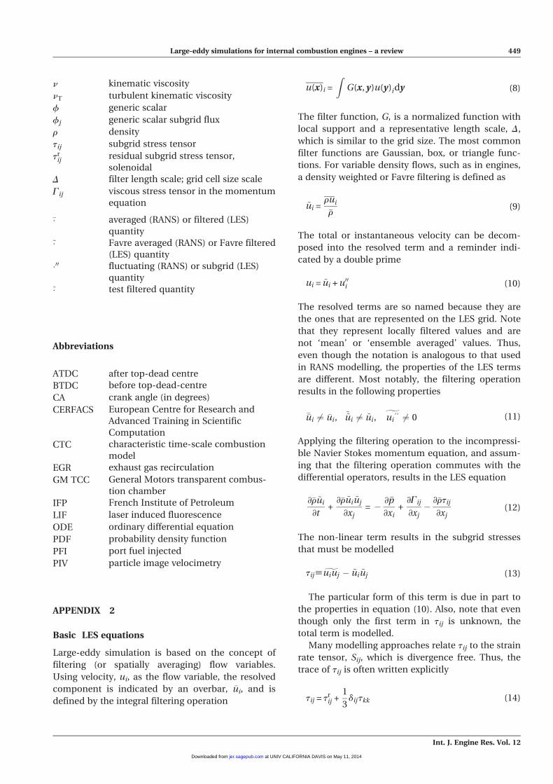
n kinematic viscosity

nT turbulent kinematic viscosity

f generic scalar

fj generic scalar subgrid flux

r density

tij subgrid stress tensor

trij residual subgrid stress tensor,

solenoidal

D filter length scale; grid cell size scale

Gij viscous stress tensor in the momentum

equation

�� averaged (RANS) or filtered (LES)

quantity

~� Favre averaged (RANS) or Favre filtered

(LES) quantity

�00 fluctuating (RANS) or subgrid (LES)

quantity

� test filtered quantity

Abbreviations

ATDC after top-dead centre

BTDC before top-dead-centre

CA crank angle (in degrees)

CERFACS European Centre for Research and

Advanced Training in Scientific

Computation

CTC characteristic time-scale combustion

model

EGR exhaust gas recirculation

GM TCC General Motors transparent combus-

tion chamber

IFP French Institute of Petroleum

LIF laser induced fluorescence

ODE ordinary differential equation

PDF probability density function

PFI port fuel injected

PIV particle image velocimetry

APPENDIX 2

Basic LES equations

Large-eddy simulation is based on the concept of

filtering (or spatially averaging) flow variables.

Using velocity, ui, as the flow variable, the resolved

component is indicated by an overbar, �ui, and is

defined by the integral filtering operation

u(x)i =

ZG(x, y)u(y)idy (8)

The filter function, G, is a normalized function with

local support and a representative length scale, D,

which is similar to the grid size. The most common

filter functions are Gaussian, box, or triangle func-

tions. For variable density flows, such as in engines,

a density weighted or Favre filtering is defined as

~ui =rui

�r(9)

The total or instantaneous velocity can be decom-

posed into the resolved term and a reminder indi-

cated by a double prime

ui = ~ui + u00i (10)

The resolved terms are so named because they are

the ones that are represented on the LES grid. Note

that they represent locally filtered values and are

not ‘mean’ or ‘ensemble averaged’ values. Thus,

even though the notation is analogous to that used

in RANS modelling, the properties of the LES terms

are different. Most notably, the filtering operation

results in the following properties

��ui 6¼ �ui, ~~ui 6¼ ~ui,gui

99 6¼ 0 (11)

Applying the filtering operation to the incompressi-

ble Navier Stokes momentum equation, and assum-

ing that the filtering operation commutes with the

differential operators, results in the LES equation

∂�r ~ui

∂t+∂�r ~ui ~uj

∂xj= � ∂�p

∂xi+∂Gij

∂xj� ∂�rtij

∂xj(12)

The non-linear term results in the subgrid stresses

that must be modelled

tij[guiuj � ~ui ~uj (13)

The particular form of this term is due in part to

the properties in equation (10). Also, note that even

though only the first term in tij is unknown, the

total term is modelled.

Many modelling approaches relate tij to the strain

rate tensor, Sij, which is divergence free. Thus, the

trace of tij is often written explicitly

tij = trij +

1

3dijtkk (14)





where, following the notation of Pope [9], trij is the

anisotropic subgrid (or residual) stress tensor. Then,

in practice, the trace is absorbed into the pressure

term and only trij is modelled. Note that this effec-

tively says the subgrid kinetic energy is unknown – a

consequence of modelling the subgrid stresses in

terms of the strain rate tensor.

For a generic scalar, f, the convection term in its

transport equation results in a term similar to tij

that also requires modelling. This term is sometimes

called the subgrid scalar flux or the turbulent scalar

mixing term and has the form

fj = fuj � �f�uj (15)

APPENDIX 3

Scale-similarity and the dynamic approach

The dynamic approach developed by Germano et al.

[11] assumes an additional filtering operation. This

is often termed the ‘test filter.’ It uses a filter func-

tion, GT, which is similar the grid or base level filter,

G, used in equation (8). Often, GT is based on a

larger length scale, 2D is common, but this is not

necessary because of equation (11). A test filtered

quantity is often denoted by a peaked overbar

du(x)i [

ZGT(x, y)u(x)idy (16)

Note, for clarity, constant density is assumed so that

the Favre and conventional filtering are the same.

Using this test filtering operation, one defines a

‘test’ level stress tensor

Tij[duiuj � �ui �uj (17)

that is analogous to the subgrid stress tensor in

equation (13). From these two stress tensors,

Germano developed the following identity

Lij = Tij �ctij (18)

where the left-hand side is

Lij = d�ui �uj � �ui �uj (19)

This quantity is known in the sense that it can be

calculated from the grid level velocities. This tensor

is known as the modified Leonard tensor since it is

similar in form but slightly different from the origi-

nal Leonard tensor. However, this difference is often

overlooked and the expression in equation (19) is

called the Leonard tensor assuming the proper

expression is known by the context in which it is

used.

The dynamic approach uses the Germano iden-

tity in equation (19) as follows. Models are proposed

for both tij and Tij. For simplicity and historical

interest, we use the Smagorinsky model

tij’� 2C1SD2 �S�� Sij +

1

3dijtkk

(20)

Tij’� 2C2S 2Dð Þ2 �S�� Sij +

1

3dijTkk (21)

where we have assumed a test filter size of 2D. Note

that the test level model is similar in form to the

subgrid model. Substituting these two models into

the Germano identity, equation (18) gives

Lij �1

3dijLkk = aijC2S � dbijC1S (22)

where, for notational convenience,

aij = � 2 2Dð Þ2 �S�� Sij, bij = � 2D2 �S

�� Sij (23)

All of the terms in equation (22) are known, except

the model coefficients, C1S and C2S. Thus, the equa-

tion can be used to solve for the coefficients. This is

the essence of the dynamic approach

However, there are still several difficulties [40]. As

written, equation (22) is an integral equation, in this

case, a Fredholm integral equation of the second

kind. Common practice is to assume the coefficient

C1S is slowly varying in space, and can be removed

from the integral that is represented by the peaked

overbar. The next common assumption is that the

two coefficients C1S and C2S are the same. This still

results in an algebraic tensor equation for a single

coefficient. Thus, the problem is over specified, so

the third common assumption is to use a minimiza-

tion procedure to solve for the model coefficient

(see Lilly [165] for details).

To summarize, the dynamic procedure consists

of the following major steps:

1. use of a test filter operation to provide informa-

tion at scales larger, but still near the subgrid

scales;

2. formulate models at the subgrid scale and the

test level scale that have a similar form;

450 C J Rutland




3. use an expression, such as the Germano identity,

that provides a relationship between the models

at the two different scales;

4. substitute the models into the expression that

can be solved for unknown model coefficients.

APPENDIX 4

The dynamic structure approach

The dynamic structure modelling approach devel-

oped by Pomraning and Rutland [40] does not use

the turbulent viscosity concept. Instead, the subgrid

stresses are modelled by a tensor coefficient, Cij,

and the subgrid kinetic energy, ksgs

tij = Cijksgs (24)

where

ksgs =1

2uiui � �ui �uið Þ (25)

The subgrid kinetic energy is obtained from a trans-

port equation. The tensor coefficient is obtained

from the dynamic approach. Assuming the coeffi-

cient can be removed from the filtering integral

gives an algebraic form of the model that is simple

to implement

Cij = 2Lij

Lkk(26)

where Lij is the modified Leonard term from equa-

tion (19). Thus, the subgrid stresses obtain their ten-

sor structure from the normalized modified Leonard

term via the dynamic procedure and their magni-

tude from the subgrid kinetic energy.

As explained here, the dynamic structure model

can be derived using the dynamic procedure.

However, it can also be viewed as a particular form

of a scale-similarity model [30]. The original scale-

similarity model was simply tij= Lij [14]. However,

this approach did not work well and required an

additional viscosity term in what is commonly called

a mixed model. In comparison to the scale-similarity

model, the dynamic model uses the subgrid kinetic

energy to determine the magnitude of the term.

More recent work has resulted in a family of

dynamic structure models (Lu et al. [12, 42]). The

primary insight was to start with equation (24) and

use other formulations for the coefficient tensor.

For example, Lu et al. found that a gradient type

approach results in

Cij = 2Gij

Gkkwhere; Gij =

∂�ui

∂xk

∂�uj

∂xk(27)

This specific form of the dynamic structure model

was shown to work well for simple flows. Testing for

engine applications is currently underway.

The dynamic structure model works very well in

practical applications. It has several important

advantages over standard dynamic viscosity-based

approaches such as T4 and T6.

1. Non-viscosity-based. By not using a turbulent

viscosity approach, the dynamic structure model

is not purely dissipative. This allows local solu-

tions that respond to the local flow conditions –

conditions that are not always dissipative.

2. An energy budget. The dynamic structure model

has a subgrid transport equation for k. This

energy budget keeps the model stable without a

turbulent viscosity. Hence, it is very robust and

works over a wide range of grid resolutions,

including practical situations in which there is

significant energy in the subgrid scales.

3. Good prediction of the subgrid stresses. The com-

ponent structure, spatial distribution, and mag-

nitude of the subgrid stresses, tij, are very well

predicted by this model. This is due to the ten-

sor coefficient that comes directly from using

the stress tensor structure in the dynamic

approach. This makes the new model a very

strong candidate for flows with more complex

physics because the subgrid terms can be used

to build other submodels.

4. Solvability. The mathematical formulation of the

new model is much sounder than the common

dynamic Smagorinsky model. The new model

satisfies basic solvability criteria that other mod-

els do not. Other LES formulations that relate tij

to Sij can be shown to violate solvability criteria

for almost any type of flow. However, the

dynamics structure model relates tij to the sub-

grid kinetic energy and this results in integral

equations that easily satisfy the solvability in

point 3. This sound mathematical formulation

adds robustness to the model so that it works

under a wide variety of flows and grid

resolutions.





large-eddy simulations for internal combustion engines - a review

Documents