large eddy simulation of the flow around an ahmed...

May 27, 2004 14:39

Proceedings of HTFED042004 ASME Heat Transfer/Fluids Engineering Summer Conference

July 11-15, 2004, Charlotte, North Carolina, USA

HT-FED2004-56325

LARGE EDDY SIMULATION OF THE FLOW AROUND AN AHMED BODY

Sinisa Krajnovic

Department of Thermo and Fluid DynamicsChalmers University of Technology

SE-412 96 GoteborgSweden

Email: [email protected]

Lars DavidsonDepartment of Thermo and Fluid Dynamics

Chalmers University of TechnologySE-412 96 Goteborg

SwedenEmail: [email protected]

ABSTRACTA new approach for large eddy simulation (LES) of the

flows around ground vehicles is demonstrated. It is based on thecharacter of the flow with large regions of recirculations ratherthan on traditional resolution requirements for the LES of wallbounded flows. Recommendations for preparing and realizationof LES for vehicle flows are presented and validated on a testcase of the flow around an Ahmed body with the 25o angle ofthe rear slanted surface. Comparison of the LES results with theexperimental data proved the validity of this new method.

INTRODUCTIONIt has been known for a long time that the shape of a ground

vehicles determines their aerodynamic properties. A modifica-tion of the shape that produces better aerodynamic properties re-quires thorough understanding of the turbulent flow around ve-hicles. Unfortunately, today after several decades of experimen-tal and numerical studies, our understanding of the flow aroundground vehicles is often limited to qualitative picture of the time-averaged large flow structures. Experimental techniques werefirst to be adopted in the studies of flows around ground vehiclesand they are still more used than numerical methods in the de-sign. Although the numerical simulations have been conductedin the automobile companies, they have failed to predict the flowsobserved in the experimental observations. Only recently the nu-merical simulations have taken over the role of some experimen-tal studies and become design tool in some of the automobile

Address all correspondence to this author.

companies (such as Volvo Cars). Both experimental and numer-ical methods have their advantages and disadvantages. Measur-ing techniques are limited to a part of the domain and are oftenused to measure time-averaged flow rather than temporal devel-opment of the instantaneous flow. The computational fluid dy-namics (CFD) can easily provide the spatial information aboutthe flow in the entire domain (virtual wind tunnel). Before wediscuss the ability of CFD to predict development of the flow intime (i.e. temporal information), it is appropriate to make someremarks about the CFD results.

Turbulent scales in the flow around ground vehicle rangefrom those of the size of the vehicle to microscopic ones. Un-fortunately most turbulent scales in this flow are small owingto high Reynolds number making resolution requirements veryhigh. This makes the solution of time-dependent Navier-Stokesequations for the flows around ground vehicles at operating ve-locities infeasible. As a result of the limitations of the computerresources, simulations of time-averaged (RANS) equations havemostly been used in the literature.

Instead of using real vehicles, very simplified (generic) ve-hicle models are often used to study how flow changes with ge-ometry. Using such an approach we can isolate few geometricproperties and study their influence on the flow.

The pioneering work by Ahmed et al (1984) had the objec-tive to study the influence of the angle between the roof and therear end slanted surface of a car with a typical fastback geometry(such as Volkswagen Golf I or Volkswagen Polo I). Their investi-gation showed a clear influence of the rear slant angle to the time-averaged flow structures. As they varied this angle they found

1 Copyright 2004 by ASME

that the flow changes the character at the angle of about 30o.Such a strange behavior of the flow with very simple change inthe geometry attracted researchers to perform further experimen-tal and numerical studies of this flow. Some of the experimentalstudies are described by Spohn and Gillieron (2002) and Lien-hart and Becker (2003). Numerical studies such as those madeby Han (1989) and described in Manceau and Bonnet (2000) areused to validate the CFD technique (often RANS simulation).Large number of RANS simulations (using different turbulencemodels) and one large eddy simulation (LES) of the flow aroundbody defined by Ahmed et al (1984) are presented by Manceauand Bonnet (2000). Only two angles of the rear slanted surface,25o and 35o, were considered in these simulations. The results ofthese simulations were compared with the experimental data pro-duced by Lienhart and Becker (2003). The main conclusion fromthese simulations was that while the simulations were relativelysuccessful in prediction of the 35o case, they were unsuccessfulin the 25o case.

The aim of this paper is to demonstrate that if carefully ap-plied, the LES can give accurate representation of the flow withthe rear slant angle of 25o case. As we already mentioned, theLES of this flow was already presented (Manceau and Bonnet(2000)) and showed poor agreement with the experimental ob-servations. This failure of LES presented in this reference showseither that LES is unable to predict this flow or that it requiresdifferent approach from that in Manceau and Bonnet (2000) andvery careful preparation and realization.

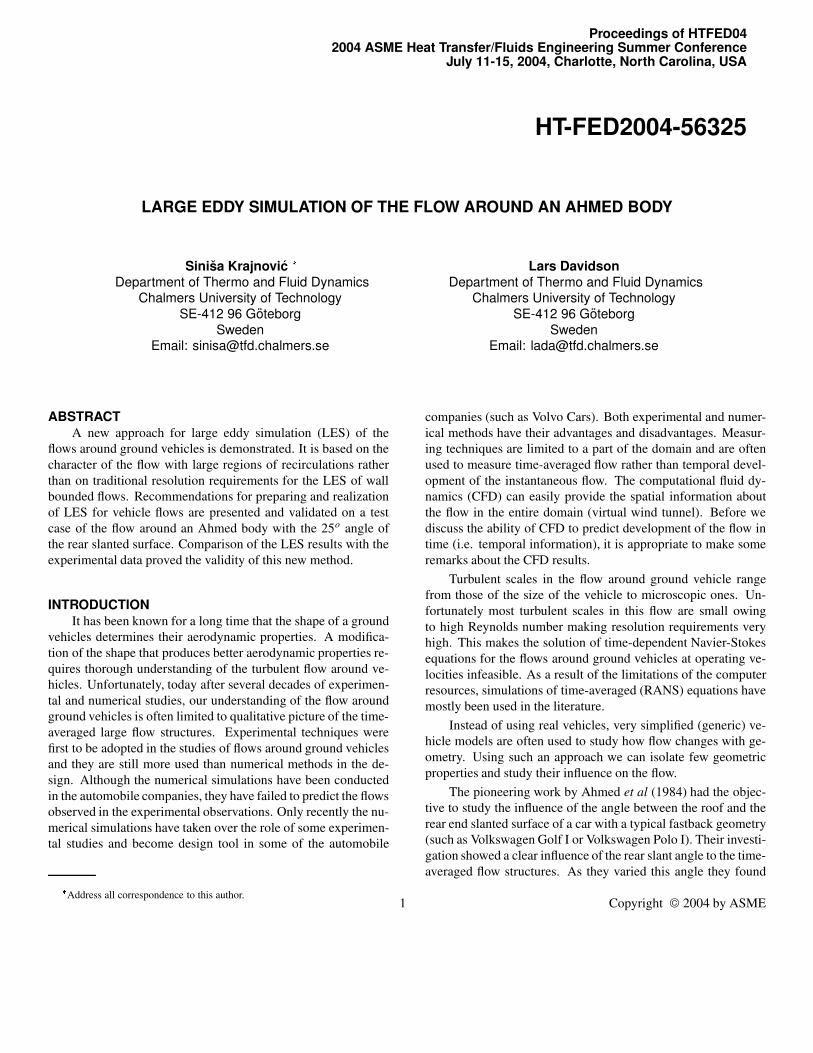
GENERIC GROUND VEHICLE BODYThe generic vehicle body was chosen to be the same as

used in the experiments by Ahmed et al (1984) and Lienhartand Becker (2003). The geometry of the body and the compu-tational domain are given in Fig. 1. All the geometric quan-tities are normalized with the body height, H, equal to 0 288m. The values of the geometric quantities are L

H 3 625,

lrH 2 928, G

H 0 697, W

H 1 35 and S

H 2 571.

The front part is rounded with a radius of RH 0 347 in the

symmetry planes y 0 and z 0. The geometry of the roundedcorners was made from the data (in form of distinct points) mea-sured at the body used in Ahmed et al (1984) and Lienhart andBecker (2003). The flow with the rear body slant angle α 25o

is considered in this paper since it was found difficult to predictin previous RANS and LES simulations (Manceau and Bonnet(2000)). This body is placed in the channel with cross section ofB F 6 493H 4 861H (width height). The cross sectionof this channel is identical with the open test section of the windtunnel used in the experiments of Lienhart and Becker (2003).The front face of the body is located at the distance of x1 7 3Hfrom the channel inlet and the downstream length between therear face of the body and the channel outlet is x2 21H. Thebody is lifted from the floor producing the ground clearance of

cH 0 174, same as in the experiments. The Reynolds num-

ber, based on the incoming velocity U∞ and the car height H,of Re 7 68 105 used in the experiments Lienhart and Becker(2003) was reduced to Re 2 105. Krajnovic and Davidson(2003) have already demonstrated successful LES of this lowerReynolds number case with no rear body slant angle, i.e. α 0o

(generic bus body). We expect that the slanted rear end will pro-duce a wider spectrum of turbulent scales that must be resolvedin LES.

MAKING LARGE EDDY SIMULATIONResolution requirements of the near-wall regions in attached

flows such as channel flow or a flat plate flow are similar to thosein direct numerical simulations. This is because the coherentstructures (so called low- and high-speed streaks) near the wallsare responsible for the most of the turbulence production in theboundary layer. Thus an accurate representation of these struc-tures is crucial for the result of the LES of the flat plate flow forexample.

Flows around bluff bodies such as that around ground vehi-cles are different from the channel or the flat plate flows. Theycontain a number of separating regions with large coherent struc-tures that contain much more turbulent energy than the near-wallstructures. Let us consider the following question. What is thesize of the smallest turbulent structures that must be resolved ina LES of the flow around ground vehicles?

In the regions of the separated flow (such as the wake be-hind the vehicle) the transport of momentum is dominated bylarge recirculating motions of the flow and the influence of thesmall near wall structures is limited. Thus the structures thatmust be resolved in this region are the smallest “large” (recircu-lating) structures. What about the attached regions in the flowaround the vehicle? The answer to this question is dependent onwhat part of the flow is our main interest. Prediction of drag isoften the main objective of the CFD study in vehicle aerodynam-ics. As the pressure drag is much larger than the friction drag andis dominated by the low pressure in the wake, prediction of thewake flow is crucial. Does this mean that it is sufficient to pre-dict the wake flow and ignore the resolution requirements for theregions located upstream from the wake? The wake flow is influ-enced by the upstream flow, but the question is how strong thisinfluence is. The boundary layer developed on the roof surfaceof the body separates at the location where the roof goes over tothe rear face of the body. We can distinct between two main situ-ations. First, the changeover from the roof to the rear face can becontinuous such as that in the circular cylinder. In that case theposition of the separation and the nature of the downstream flowis determined by the upstream history of the flow. The secondsituation is when the geometry defines the separation of the flowsuch as in the generic car body studied in this paper. How big isthe influence of the upstream flow on the wake in this case? Is


the resolution of the upstream boundary layer equally importanthere as in the case with the continuous changeover in the surfacegeometry? We believe that in this case the influence of the ge-ometry is much larger than that of the upstream history of theflow.

OUR APPROACHAlthough we assume that in the flow around our generic

body, the upstream boundary layer has limited influence on theflow in the wake, we cannot neglect it. Thus we should try to pre-dict the near wall region as good as possible. Unfortunately thenear wall coherent structures decrease in size with the Reynoldsnumber and for the Reynolds number used in the experimentsby Lienhart and Becker (2003), the task of resolving these struc-tures is overwhelming (see Krajnovic (2002) for the estimate ofthe computational cost for the resolution of the near-wall struc-tures in the flow around ground vehicle body).

We have already assumed that the geometry rather than theupstream flow defines the flow in the wake. Here we make an-other assumption. The magnitude of the Reynolds number isless important for the recirculating flow in the wake than forthe boundary layer. Together with the dependence of the wakeflow on the geometry this means that we can reduce the Reynoldsnumber in our LES and obtain a flow similar to that in the exper-iment that is characterized by the higher Reynolds number. Weemphasize that these are still only hypothesis.

If our hypothesis of Reynolds number independence of thewake flow is correct, how much can we lower the Reynolds num-ber and still obtain this independence? This is not clear but thesimulated flow on the roof should be as similar as possible tothat in the experiment at high Reynolds number. Thus if thehigh Reynolds number roof flow does not separate at the lead-ing edge, our simulated low Reynolds number flow should notseparate or should have as small separated regions as possible.Our knowledge about the dependence of the Reynolds numberand the shape of the front of the ground vehicle (i.e. rounded-ness of the leading edges) is poor and is limited to the depen-dence of the drag coefficient on the Reynolds number and theroundedness of the leading edges of the prismatic bodies (Cooper(1985)). As the information about the flow on the roof, lateralsides and the under-body is not available from the experiments,we don’t know if the flow separates on these surfaces. However,we can draw some conclusions from our previous LES of theflow around a similar body (Krajnovic and Davidson (2003)). Asthe front of the body is more rounded and the Reynolds num-ber is higher in Lienhart and Becker (2003) (body studied in thispaper) than in Krajnovic and Davidson (2003) we conclude thatthe separated regions, if they exist, are smaller around the frontof the body here than on the body in Krajnovic and Davidson(2003). Krajnovic and Davidson (2003) showed that LES canpredict the flow around the ground vehicle body that is character-

ized with Reynolds number of about 2 105 (based on the hightof the body and the velocity at the inlet). Thus we choose for ourLES the Reynolds number of 2 105 instead of the experimental7 68 105 (thus about four times lower LES Reynolds numbercompared to the experimental one).

PREPARATION AND REALIZATION OF LESMost LES of the flow around bluff bodies are using struc-

tured hexahedral meshes which give better accuracy than for ex-ample tetrahedral meshes. Making a structured hexahedral meshso that the computational cells are concentrated where they areneeded is far from trivial even around relatively simple bluffbody such as the ground vehicle body studied in this paper. Pro-viding the optimal structured mesh for the detailed passenger carwould be quite a challenge.

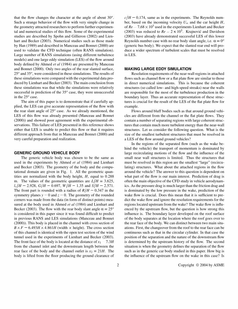
Here we shall demonstrate one of the approaches that canbe used to concentrate most of the cells in the region around thebody. Instead of using only H grid topology that spread the fineresolution in the boundary layer of the body all the way to theboundaries of the wind tunnel, we use a combination of O andC grid topologies (see Fig. 2) that makes local refinement of thegrid possible. The topology of the grid consists of an O grid,with a thickness of 0 1H and a C grid around the O grid (see Fig.2). An additional ’dummy’ car surface was made around the realcar and the O grid was projected on these two surfaces. The restof the blocking structures was made using H grids. This strategyresulted in the following distribution of the computational cells.The O grid ( i.e. the region in a belt of thickness 0 1H aroundthe body) contained 4 4 and 7 5 million cells of totally 9 6 and16 5 million cells in the medium and the fine grids, respectively.The region containing the O and the C grids together (i.e. theregion in a belt of thickness 0 28H around a car) hold 6 3 and10 8 million cells in the medium and the fine grids, respectively.

Unlike the results of steady RANS simulations, the resultsof time-dependent LES are dependent on the time where we startto monitor our results (i.e. when the fully developed flow is ob-tained). Unfortunately, in the LES of the flow around groundvehicles the fully developed flow is unknown and must be com-puted. The initial fully developed flow is often computed fromthe fluid at rest (as in this paper) or from a previous solution ofRANS simulation. How do we know that the flow has becomefully developed? Probably, the only way to be sure that the flowhas developed is the ’a posteriori’ one (i.e. after the entire simu-lation). Such a test could prove that the mean, RMS values andthe spectral picture of the solution are not dependent on the po-sition in time where we started sampling of the solution. As weneed to start the time averaging before we can perform the ’aposteriori’ test, some approximate method must be used to en-sure that the characteristics of the flow are not changing. Wemonitored the time required for the fluid particle to travel fromthe front to the rear face of the car body. We then computed the


Inflow Outflow

1

Lateral walls

1

Figure 1. Schematic representation of the computational domain with vehicle body.

C-grid

O-grid

D

Figure 2. The computational mesh in symmetry plane y 0. D indi-cates the position of the dummy surface. View from the lateral side.

mean and the RMS values of the global quantities (aerodynamicforces) and local variables (velocity components and pressure inseveral points in and around the wake behind the body) for thistime interval. The Fourier transforms of both global and localquantities were computed but because of the relatively short timesequences we could rely only on the high frequency events. Thetime averaging was started when there were no significant dif-ferences in the mean and the instantaneous information betweentwo sequential time sequences. Computational cost for obtain-ing the fully developed flow is significant and for the simulationspresented in this paper the computational time for obtaining fullydeveloped conditions were roughly one fourth of the total time ofthe simulations.

When the flow has evolved to become fully developed, mon-itoring of the instantaneous results and their averaging can begin.Numerical time steps in LES are short to retain accuracy. Theshort time steps lead to large number of time steps for resolvingthe low frequency events and the time averaging. Our experi-

ence is that the number of time steps required for resolving thelow frequency events is larger than that needed for obtaining ofthe time-averaged results (see Krajnovic and Davidson (2003)).Thus in this work we shall confine our simulation to providetime-averaged results that are not a functions of time (i.e. theaveraging time is long enough) rather than resolve all low fre-quency turbulence events. The symmetry of the flow around thesymmetry plane (y 0 plane) was used in this paper as a proofof long enough averaging time.

GOVERNING EQUATIONS AND SUBGRID-SCALEMODELING

The governing LES equations are the incompressibleNavier-Stokes and the continuity equations filtered with the im-plicit spatial filter of characteristic width ∆ (∆ is the grid resolu-tion in this work):

∂ui

∂t ∂∂x j

uiu j ! 1

ρ∂p∂xi ν

∂2ui

∂x j∂x j ∂τi j

∂x j(1)

and

∂ui

∂xi 0 (2)

Here, ui and pi are the resolved velocity and pressure, respec-tively, and the bar over the variable denotes filtering.

These equations are derived applying a filtering operation

fxi #"

Ωfx $i G xi % x $i dx $i (3)

on the Navier-Stokes and the continuity equations. Here G is atop hat filter function and Ω represents the entire flow domain.The filtered variables in the governing Eqs. (1) and (2) are ob-tained implicitly through the spatial discretization.


The goal of the filtering is to decompose the fluid motioninto a large-scale component that are resolved and the small sub-grid scale (SGS) that are modeled. The influence of the smallscales of the turbulence on the large energy carrying scales inEq. (1) appears in the SGS stress tensor, τi j uiu j uiu j. The al-gebraic eddy viscosity model originally proposed by Smagorin-sky (1963) is used in this paper for its simplicity and low compu-tational cost. The Smagorinsky model represents the anisotropicpart of the SGS stress tensor, τi j , as:

τi j 13

δi jτkk & 2νsgsSi j (4)

where νsgs Cs f ∆ 2 ' S ' is the SGS viscosity,

Si j 12 ( ∂ui

∂x j ∂u j

∂xi ) (5)

is the resolved rate-of-strain tensor and ' S ' +* 2Si jSi j , 12 . f in

the expression for the SGS viscosity is the van Driest dampingfunction

f 1 exp ( y -25 ) (6)

Using this damping function, wall effects are partially taken intoaccount by ’damping’ the length scale l Cs f ∆ near to thewalls. The value of Cs 0 1 previously used for bluff-bodyflows (Krajnovic and Davidson (2002)) and flow around simpli-fied bus (Krajnovic (2002), Krajnovic and Davidson (2003)) isused in this work. The filter width, ∆, is defined in this work as∆ ∆1∆2∆3 1 . 3, where ∆i are the computational cell sizes inthree coordinate directions.

BOUNDARY CONDITIONS AND NUMERICAL DETAILSThe average turbulent intensity at the inlet of the wind tun-

nel used in the experiments of Lienhart and Becker (2003) was0 25%. A uniform velocity profile constant in time was thusused as the inlet boundary condition in our LES. The convec-tive boundary condition ∂ui

∂t Uc

∂ui∂x 0 was used at

the downstream boundary. Here, Uc was set equal to the in-coming mean velocity, U∞. The lateral surfaces and the ceilingwere treated as slip surfaces using symmetry conditions (∂u

∂z

∂w∂z v 0 for the lateral sides and ∂u

∂z ∂v

∂z w 0

for the ceiling). This boundary condition is different from theexperimental one where the test section had a floor but no lateralsides or ceiling. The consequence of this boundary condition isthat the flow across the lateral sides and the ceiling is permitted

in the experiment but not in the simulation resulting in different’effective’ blocking of the cross section. This will probably havesome influence on the aerodynamic forces. No-slip boundaryconditions were used on the surface of the body and the instan-taneous wall functions based on the log-law (see Krajnovic andDavidson (2001) for details) were applied on the channel floor.

Numerical accuracy was established by making three LESon different computational grids containing 3 5, 9 6 and 16 5millions nodes. The time step was 1 10 / 4, giving a maximumCFL number of approximately 0 9. The averaging time, tU∞

H,

in the simulations was 38 2 (110 % 000 time steps).

NUMERICAL METHODEquations (1) and (2) are discretized using a 3D finite

volume method for solving the incompressible Navier-Stokesequations using a collocated grid arrangement (Davidson andFarhanieh (1995)). Both convective and viscous plus sub-grid fluxes are approximated by central differences of second-order accuracy. The time integration is done using the Crank-Nicolson second-order scheme. Although no explicit dissipationis added to prevent odd-even decoupling, an implicit dissipationis present. This is done by adding the difference between thepressure gradient at the face and the node. It can be shown thatthis term is proportional to the third derivative of pressure, i.e.∂3 p∂x3

i . This term corresponds to Rhie-Chow dissipation (Rhieand Chow (1983)). The SIMPLEC algorithm is used for thepressure-velocity coupling. The code is parallelized using blockdecomposition and the PVM and MPI message passing systems(Nilsson and Davidson (1998)).

RESULTSAlthough we have collected large amount of results we can

present only small fraction in this paper due to space limitations.We chose to present comparison of our LES results and the ex-perimental data for the flow around the rear part of the body.An accurate prediction of time-averaged flow above the slantedsurface implies an accurate prediction of the corresponding in-stantaneous flow. Thus we describe the time instantaneous flow.

COMPARISON OF THE LES RESULTS WITH THE EX-PERIMENTAL DATA

This section presents comparison of our LES results withthe experimental data of Lienhart and Becker (2003). Although,we have made comparison of all the profiles available in the datafiles provided from this experimental work, there is no place inthis paper to present all the results. Thus we have chosen topresent only profiles in the center plane y 0 that were usedfor comparison in previous CFD studies (Manceau and Bonnet(2000)).


Velocity and Reynolds stresses were measured using a two-component laser-Doppler anemometer (LDA). As we compareLES and experimental profiles we should keep in mind thatthe experimental data comes from several different experimentalruns. As we will show later, we have found some discrepanciesbetween our LES profiles and experimental data for some po-sitions which came from one data set and no discrepancies forother positions which were almost identical to the former onesbut the experimental data came from another set of experiments.We shall discuss these differences in the following text.

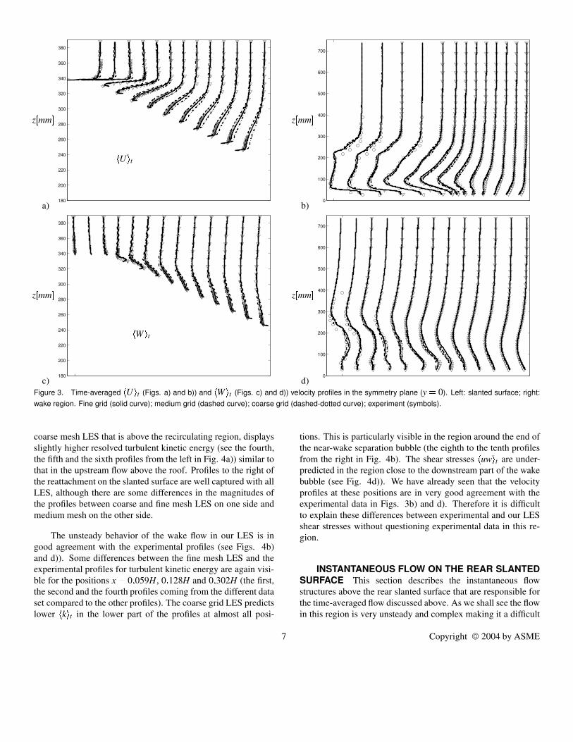
Comparison of the velocity profiles and Reynolds stresses inthe plane y 0 are presented in Figs. 3 and 4. Figure 3a) presentsstreamwise velocity profiles 0 U 1 t on the roof and the slantedsurface for positions between x 2 0 844H and x 2 0 01H(from left to right) where the space difference between two pro-files is ∆x 0 07H. The experimental profiles for positionx 3 0 774H are not available and the LES profiles are presentedhere only to show the development of the predicted boundarylayer at this position. Fine mesh LES (denoted with solid line)overlaps the experimental profiles at all positions except perhapsat the positions on the roof of the body (i.e. x 4 0 844H and 0 705H). The discrepancies on the roof are probably due todifferent Reynolds numbers in experiments and our simulations.Although the flow separates on the leading edge of the front endof the body in our simulation (not shown here), the separationsregion is very thin in both streamwise and wall normal direc-tions. There are no experimental observations of the flow aroundthe front part of the body at the high Reynolds number, but it isreasonable to expect that the separation region becomes thinneras the Reynolds number is increased. Thus the flow on the roof isprincipally turbulent boundary layer and therefore defined by theviscosity. The Reynolds number in our LES is about four timeslower than in the experiments resulting in differences in bound-ary layer thicknesses. The influence of the Reynolds number isreduced already at the position directly after the upstream sharpedge of the slanted surface (i.e. x ! 0 635H in Fig. 3a) and thegeometry starts to dictate the downstream flow. The coarse meshsimulation (dashed-dotted curve in the figure) predicts very un-realistic flow with oscillations far above the boundary layer (seethe third profile from the left in Fig. 3a)). It is interesting toobserve how the change from attached to separated flow down-stream of the fourth profile position (x 5 0 635H) smoothesout these oscillations. Differences between the three LES andthe experimental data are smaller in the region of the separationbubble than in the region after the reattachment on the slantedsurface (see Fig. 3a)). The coarse mesh simulation predicts toohigh momentum above the slanted surface in the region after thereattachment. This shows again that the resolution of the nearwall structures is much more important in the attached flow re-gion above the lower part of the slant than in the recirculationregion above the upper part of the slanted surface.

The 0W 1 t velocities along the slanted surface are for all three

LES in very good agreement with the experimental profiles (seeFig. 3c)). Also here there are some differences between simula-tions but these appear to be smaller due to smaller magnitude ofthe 0W 1 t velocities compared to 0 U 1 t velocities.

Figures 3b) and d) present 0 U 1 t and 0W 1 t velocity profilesin the wake region behind the body for positions x equal with0 059H, 0 128H, 0 132H, 0 302H, 0 306H, 0 479H, 0 653H,0 826H, H, 1 174H, 1 521H, 1 868H and 2 215H from left toright, respectively. Let us first consider all profiles at all posi-tions except x 0 059H, 0 128H and 0 302H. Although the LESusing fine mesh gives almost exact representation of the experi-mental profiles, all three LES predicted profiles are in very goodagreement with the experimental data. Coarse LES have someproblems to give accurate representation of the lower recirculat-ing region (see profiles at x 0 132H and 0 306H in 3b) (i.e. thethird and the fifth profiles from the left, respectively)) but alreadythe medium simulation capture these regions very well. Let usnow return to the remaining three positions (the first, the secondand the fourth profiles from the left, i.e. x 0 059H, 0 128H and0 302H). The experimental data for these profiles are denotedhere with circles and comes from a different data set than theone that contains all other profiles in the wake. The experimentalprofiles for these positions are provided only up to z 388mmcompared to other profiles that goes up to z 738mm. All LESsimulations are in relatively poor agreement with experiment inthe upper part of the velocities profiles at these positions (seeFig. 3b) and d)). Profiles x 0 128H (the second profile fromthe left) and x 0 302H (the fourth profile from the left) are lo-cated at positions that are only 1mm from profiles in the first dataset, x 0 132H (the third profile) and x 0 306H (the fifth pro-file), respectively. Still the flow in the experimental data changespretty much between these almost identical positions. Besides,our LES using fine mesh gives exact representation of the exper-imental profiles from the first data set. Thus we conclude thatsomething is wrong with the experimental data for the seconddata set (i.e. at the positions x 0 059H, 0 128H and 0 302H).

Figure 4 presents comparison between experimental andLES time-averaged resolved turbulent kinetic energy 0 k 1 t andshear stresses 0 uw 1 t in the center plane y 0. We shall first con-centrate on the flow along the slanted surface in Figs. 4a) andc). The oscillations in the coarse LES of the flow above the roof(the first, the second and the third profiles from the left) foundin the velocity field are amplified here (see the third profile fromthe left in Figs. 4a) and c)). Besides the turbulent kinetic en-ergy is overpredicted in this coarse mesh simulation in the roofflow (see first three profiles from the left in Fig. 4a)). As wemove downstream and pass the separation edge (profiles numberfour, five etc), the oscillations in the coarse LES disappear. Allthree LES produce slightly lower turbulent kinetic energy thanthe experiment in the region of recirculating flow (see Fig. 4a))indicating that the experimental flow is slightly more unsteadythan the simulated one. The part of the predicted profiles using


a)180

200

220

240

260

280

300

320

340

360

380

PSfrag replacements

z 6mm 78U 9 t

b)0

100

200

300

400

500

600

700

PSfrag replacements

z 6mm 7

U t

c)180

200

220

240

260

280

300

320

340

360

380

PSfrag replacements

z 6mm 78W 9 t

d)0

100

200

300

400

500

600

700

PSfrag replacements

z 6mm 7

W t

Figure 3. Time-averaged 0 U 1 t (Figs. a) and b)) and 0W 1 t (Figs. c) and d)) velocity profiles in the symmetry plane (y 0). Left: slanted surface; right:wake region. Fine grid (solid curve); medium grid (dashed curve); coarse grid (dashed-dotted curve); experiment (symbols).

coarse mesh LES that is above the recirculating region, displaysslightly higher resolved turbulent kinetic energy (see the fourth,the fifth and the sixth profiles from the left in Fig. 4a)) similar tothat in the upstream flow above the roof. Profiles to the right ofthe reattachment on the slanted surface are well captured with allLES, although there are some differences in the magnitudes ofthe profiles between coarse and fine mesh LES on one side andmedium mesh on the other side.

The unsteady behavior of the wake flow in our LES is ingood agreement with the experimental profiles (see Figs. 4b)and d)). Some differences between the fine mesh LES and theexperimental profiles for turbulent kinetic energy are again visi-ble for the positions x 0 059H, 0 128H and 0 302H (the first,the second and the fourth profiles coming from the different dataset compared to the other profiles). The coarse grid LES predictslower 0 k 1 t in the lower part of the profiles at almost all posi-

tions. This is particularly visible in the region around the end ofthe near-wake separation bubble (the eighth to the tenth profilesfrom the right in Fig. 4b). The shear stresses 0 uw 1 t are under-predicted in the region close to the downstream part of the wakebubble (see Fig. 4d)). We have already seen that the velocityprofiles at these positions are in very good agreement with theexperimental data in Figs. 3b) and d). Therefore it is difficultto explain these differences between experimental and our LESshear stresses without questioning experimental data in this re-gion.

INSTANTANEOUS FLOW ON THE REAR SLANTEDSURFACE This section describes the instantaneous flowstructures above the rear slanted surface that are responsible forthe time-averaged flow discussed above. As we shall see the flowin this region is very unsteady and complex making it a difficult


a)240

260

280

300

320

340

360

380

PSfrag replacements

z 6mm 78k 9 t

b)0

100

200

300

400

500

600

700

PSfrag replacements

z 6mm 7

k t

c)240

260

280

300

320

340

360

380

PSfrag replacements

z 6mm 78uw 9 t

d)0

100

200

300

400

500

600

700

PSfrag replacements

z 6mm 7

uw t

Figure 4. Time-averaged resolved turbulent kinetic energy (Figs. a) and b)) and shear stress (Figs. c) and d)). Left: slanted surface; right: wake region.Fine grid (solid curve); medium grid (dashed curve); coarse grid (dashed-dotted curve); experiment (symbols).

candidate for RANS modeling. The fluid separates at the sharpedge between the roof surface and the slanted rear surface (seeFig. 5). Coherent structures that extend in the spanwise directionare formed as a result of this separation. The axes of these struc-tures are parallel with the edge of separation along the middlepart of the edge between the roof and the slanted surface. Thosevortices that are born close to the corners of the slanted surfaceare tilted so that they travel toward the center of the slanted sur-face. When the spanwise vortices are convected downstream theymerge with each other forming slightly larger vortices such as λ1in Fig. 5a). Next step in their development is to merge with eachother and become bigger such as λ1 in Fig. 5b) before their tipis lifted from the surface and form hairpin like vortices (see λ1in Fig.5c)). Their lifespan as hairpin vortices with both legs onthe slanted surface (such as λ2 in Fig.5a)) is short. One of theirlegs separates from the surface or is just being broken such as

in λ2 in Fig. 5b). Finally close to the re-attachment around thehalf length of the slanted surface the other leg of the vortex isdestroyed (see λ2 in Fig. 5c)) with only small partition continu-ing downstream and possibly entering the wake region. Vorticestraveling downstream are colored with white and those travelingupstream are colored with black. As we can see the recircula-tion region contains mainly the vortices that travel downstream.They are much stronger than the black-colored vortices close tothe surface which are traveling upstream.

The flow coming from the lateral side up over the slant lat-eral edge separates with high velocity resulting in pressure deficitalong the slant edge on the slanted surface side. The fluid rolesover the slanted surface from the lateral side to the slanted sur-face. This takes place on two levels. One thin cone like vortex Tr1is formed close to the slant edge with a larger vortex Tr3 aroundit (see Fig. 6). These vortices remind of a gearwheel mechanism


a)

λ1

λ2

λ3

Tr3

b)

λ1

λ2

λ3

c)

λ1

λ2

λ3

Figure 5. The isosurface of the instantaneous second invariant of thevelocity gradient, Q 6500. The time difference between two picturesis tU∞

H 0 055. Flow is from left to right and the view is from the

later side of the body. Vortices are colored by the streamwise velocity.The white vortices are traveling downstream and the black vortices aretraveling upstream.

although they are not actually driving each other. The mantle ofthe vortex Tr3 (gearwheel number three) that starts as the shearlayer on the slanted edge follows the conical path and ends onthe slanted surface before it reaches the slanted edge. When itsmantle leaves the surface again to continue counter clockwiserotation, it draws the neighboring fluid particles in the upwarddirection. On the other side the vortex Tr1 (gearwheel numberone) re-attaches on the slanted surface drawing its neighboringfluid particles down toward the surface. These two mechanismsproduces the third cone-like vortex Tr2 (gearwheel number two)with clockwise direction of rotation (see Fig. 6). Only two ofthese vortices (i.e. Tr2 and Tr3) were observed in previous studiesby Ahmed et al (1984) and Spohn and Gilleron (2002).

This motion of the fluid from the lateral side to the slantedsurface influences partly the upstream flow so that the trailingvortices can be observed upstream of the separation edge be-tween the roof and the slanted surface of the body (see Fig. 5).Here we say ’partly’ because some coherent structures are in-duced already at the front of the lateral edge of the body andconvected downstream (not shown here). Similar structures wereobserved in Spohn and Gillieron (2002) where the motion of fluidfrom the lateral side to the roof was observed at position 0 25Hupstream the separation edge.

Let us now return to the spanwise vortices close to the uppercorners of the slanted surface (such as λ3 in Fig. 5). As we al-ready mentioned their axes are tilted with respect to the spanwiseedge between the roof and the slanted surfaces. This behavior iscaused by the cone like shape of the vortex Tr3. As it propagatesdownstream it grows in the diameter pushing the λ-vortices awayfrom the slant edge. The resulting orientation of the λ-vorticesclosest to the Tr3 is toward the center of the slanted surface.

CONCLUSIONSOur hypothesis of the partial Reynolds number indepen-

dence of some vehicle flows was confirmed. Although this wasdemonstrated only for a body with separations strongly definedby the geometry, this shows that LES has large potential in exter-nal vehicle aerodynamics.

Using our LES results we have described highly unsteadyturbulent mechanisms above the slanted surface. Large differ-ences in the turbulent length scales and the lengths of the turbu-lence events were registered in this part of the flow.

ACKNOWLEDGMENTSThis work was supported by the FLOMANIA project. The

FLOMANIA (Flow Physics Modeling - An Integrated Ap-proach) is a collaboration between Alenia, AEA, Bombardier,Dassault, EADS-CASA, EADS-Military Aircraft, EDF, NU-MECA, DLR, FOI, IMFT, ONERA, Chalmers University, Im-perial College, TU Berlin, UMIST and St. Petersburg State Uni-versity. The project is funded by the European Union and ad-


Tr3 : ω ;x <

Tr2 : ω =x < Tr1 : ω ;x <Figure 6. The isosurface of the instantaneous second invariant of thevelocity gradient, Q 6500. View is from behind of the right slant edge.Note that only core parts of the cone vortices are shown. The cone vor-tices are colored by the vorticity component in the streamwise directionωx. Vortices colored with black and white have clockwise and contourclockwise direction of rotation, respectively.

ministrated by the CEC, Research Directorate-General, GrowthProgramme, under Contract No. G4RD-CT2001-00613. Com-puter time on the Linux cluster, provided by the NSC (NationalSupercomputer Center in Sweden), is gratefully acknowledged.

REFERENCESAhmed, S. R., G. Ramm, and G. Faltin (1984). Some salient

features of the time averaged ground vehicle wake. SAEPaper 840300.

Cooper, K. R. (1985). The effect of front-edge rounding andrear edge shaping on the aerodynamic drag of bluff vehi-cles in ground proximity. SAE Paper No. 850288.

Davidson, L. and B. Farhanieh (1995). CALC-BFC: A finite-volume code employing collocated variable arrangementand cartesian velocity components for computation offluid flow and heat transfer in complex three-dimensionalgeometries. Report 95/11, Dept. of Thermo and Fluid Dy-namics, Chalmers University of Technology, Gothenburg.

Han, T. (1989). Computational analysis of three-dimensionalturbulent flow around a bluff body in ground proximity.AIAA Journal 27(9), 1213–1219.

Krajnovic, S. (2002). Large Eddy Simulations for Computingthe Flow Around Vehicles. Ph. D. thesis, Dept. of Thermoand Fluid Dynamics, Chalmers University of Technology,Gothenburg.

Krajnovic, S. and L. Davidson (2001). Large eddy simula-tion of the flow around a ground vehicle body. In SAE2001 World Congress, SAE Paper 2001-01-0702, Detroit,Michigan, USA.

Krajnovic, S. and L. Davidson (2002). Large eddy simulationof the flow around a bluff body. AIAA Journal 40(5), 927–936.

Krajnovic, S. and L. Davidson (2003). Numerical Study ofthe Flow Around the Bus-Shaped Body. ASME: Journalof Fluids Engineering 125, 500–509.

Lienhart, H. and S. Becker (2003). Flow and turbulente struc-ture in the wake of a simplified car model. SAE Paper2003-01-0656.

Manceau, R. and J.-P. Bonnet (2000). 10th joint ERCOFTAC(SIG-15)/IAHR/QNET-CFD Workshop on Refined Tur-bulence Modelling. Poitiers.

Nilsson, H. and L. Davidson (1998). CALC-PVM: A parallelSIMPLEC multiblock solver for turbulent flow in complexdomains. Internal report 98/12, Department of Thermoand Fluid Dynamics, Chalmers University of Technology,Gothenburg.

Rhie, C. and W. Chow (1983). Numerical study of the turbu-lent flow past an airfoil with trailing edge separation. AIAAJournal 21(11), 1525–1532.

Smagorinsky, J. (1963). General circulation experiments withthe primitive equations. Monthly Weather Review 91(3),99–165.

Spohn, A. and P. Gillieron (2002). Flow separations generatedby a simplified geometry of an automotive vehicle. In IU-TAM Symposium: Unsteady Separated Flows, April 8-12,Toulouse, France.


large eddy simulation of the flow around an ahmed...

Documents