large eddy simulation of primary liquid-sheet breakup
TRANSCRIPT

LARGE EDDY SIMULATION OF PRIMARY
LIQUID-SHEET BREAKUP
by
Thibault Pringuey
Trinity Hall
University of Cambridge
This dissertation is submitted for the degree of
Doctor of Philosophy
April 2012

Dedicated to my wife Imelda
and
to my grandfather Maurice.
i

Declaration
This dissertation is the result of my own work and includes nothing which is the
outcome of work done in collaboration except where specifically indicated in the text.
The dissertation contains approximately 63500 words, 98 figures and 22 tables.
Thibault Pringuey
Hopkinson Laboratory, University of Cambridge,
Wednesday, 4th of April, 2012
ii

Acknowledgements
I am very grateful to all people who supported me during this PhD project. First
of all, I would like to thank my supervisor, Prof. Stewart Cant, for his invaluable
help, his enthusiasm and his constant encouragement. Thanks to his availability,
his technical expertise and his great sense of humour this research project has been
a very positive and enjoyable experience.
I am also thankful to the senior staff of the Combustion department of Rolls-
Royce plc. for funding this work. In particular, I would like to thank Jon Gregory,
John Moran and Ken Young who made this project possible. My thanks also go to
Marco Zedda and Steve Harding (Rolls-Royce plc.) for their technical input.
I would like to thank Dr. Thomas Ruberg for his useful advice on computational
integration. In addition, I thank Prof. Rickard Bensow and Prof. Christer Fureby
(Chalmers University of Technology) for welcoming me in Sweden and for our very
interesting technical discussions. I am also thankful to Prof. Peter Stephan (Tech-
nical University of Darmstadt) and his group for the visit of their experimental
facilities and our discussions on the capability of OpenFOAM. The support received
from the administrators of Cambridge’s High Performance Computing facilities is
also gratefully acknowledged.
I would like to express my gratitude to all my colleagues of the laboratory for
the pleasant working atmosphere of the Hopkinson Students’ Room. In particular,
I thank Camille Letty, Chris Bohn, Andrea Maffioli, Teresa Leung, Adam Comer,
Ryan Harper, Robert Gordon, Alexandre Neophytou, Andrea Pastore, Giulio Borgh-
iii

esi, Davide Cavaliere and Kieran Hegarty.
My final thanks go to my wife Imelda, for her advice and constant support along
the whole project, and to my daughters Claire and Eleonore — born in the course
of this PhD — who kept on cheering (day and night).
iv

Abstract
This research project aims at providing the aeronautical industry with a modelling
capability to simulate the fuel injection in gas turbine combustion chambers.
The path to this objective started with the review of state-of-the-art numerical
techniques to model the primary breakup of liquid fuel into droplets. Based on this
and keeping in mind the requirements of the industry, our modelling strategy led to
the generation of a mass-conservative method for efficient atomisation modelling on
unstructured meshes. This goal has been reached with the creation of high-order
numerical schemes for unstructured grids, the development of an efficient numeri-
cal method that transports the liquid-vapour interface accurately while conserving
mass and the implementation of an algorithm that outputs the droplet boundary
conditions to separate combustion codes.
Both high-order linear and WENO schemes have been created for general polyhe-
dral meshes. The notorious complexity of high-order schemes on 3D mixed-element
meshes has been handled by the creation of a series of algorithms. These include
the tetrahedralisation of the mesh, which allows generality of the approach while
remaining efficient and affordable, together with a novel approach to stencil gener-
ation and a faster interpolation of the solution. The performance of the scheme has
been demonstrated on typical two-dimensional and three-dimensional test cases for
both linear and non-linear hyperbolic partial differential equations.
The conservative level set method has been extended to unstructured meshes and
its performance has been improved in terms of robustness and accuracy. This was
v

achieved by solving the equations for the transport of the liquid volume fraction
with our novel WENO scheme for polyhedral meshes and by adding a flux-limiter
algorithm. The resulting method, named robust conservative level set, conserves
mass to machine accuracy and its ability to capture the physics of the atomisation
is demonstrated in this thesis.
To be readily applicable to the simulation of atomisation, the novel interface-
capturing technique has been embedded in a framework — within the open source
CFD code OpenFOAM — that solves the velocity and pressure fields, outputs
droplet characteristics and runs in parallel. In particular, the production of droplet
boundary conditions involves a set of routines handling the selection of drops in the
level set field, the calculation of relevant droplet characteristics and their storage into
data files. An n-halo parallelisation method has been implemented in OpenFOAM
to perform the computations at the expected order of accuracy.
Finally, the modelling capability has been demonstrated on the simulation of
primary liquid-sheet breakup with relevance to fuel injection in aero-engine com-
bustors. The computation has demonstrated the ability of the code to capture the
physics accurately and further illustrates the potential of the numerical approach.
vi

Contents
Contents . . . . . . . . . . . . . . . . . . . . . . . . . . . . . . . . . . . . . vii
List of figures . . . . . . . . . . . . . . . . . . . . . . . . . . . . . . . . . . xiii
List of tables . . . . . . . . . . . . . . . . . . . . . . . . . . . . . . . . . . xvii
Nomenclature . . . . . . . . . . . . . . . . . . . . . . . . . . . . . . . . . . xx
1 Introduction 1
1.1 The aeronautical application . . . . . . . . . . . . . . . . . . . . . . . 2
1.2 Motivations . . . . . . . . . . . . . . . . . . . . . . . . . . . . . . . . 3
1.3 Approaches to study the primary breakup . . . . . . . . . . . . . . . 3
1.4 Numerical modelling of atomisation . . . . . . . . . . . . . . . . . . . 4
1.4.1 Numerical framework . . . . . . . . . . . . . . . . . . . . . . . 4
1.4.2 Interface description . . . . . . . . . . . . . . . . . . . . . . . 5
1.4.3 Treatment of singularities . . . . . . . . . . . . . . . . . . . . 5
1.5 Aim of the present work . . . . . . . . . . . . . . . . . . . . . . . . . 6
1.6 Outline of the thesis . . . . . . . . . . . . . . . . . . . . . . . . . . . 7
2 Physics of primary breakup 8
2.1 Fundamental forces and dimensional analysis . . . . . . . . . . . . . . 8
2.2 Early research interest . . . . . . . . . . . . . . . . . . . . . . . . . . 9
2.3 Round liquid jet breakup . . . . . . . . . . . . . . . . . . . . . . . . . 10
2.3.1 Jet breakup regimes . . . . . . . . . . . . . . . . . . . . . . . 10
2.3.2 Spray structure . . . . . . . . . . . . . . . . . . . . . . . . . . 11
vii

2.3.3 Properties of round jet sprays . . . . . . . . . . . . . . . . . . 13
2.3.4 Ligament formation . . . . . . . . . . . . . . . . . . . . . . . . 13
2.4 Liquid sheet breakup . . . . . . . . . . . . . . . . . . . . . . . . . . . 16
2.4.1 Natural disintegration . . . . . . . . . . . . . . . . . . . . . . 17
2.4.2 Assisted non-linear disintegration . . . . . . . . . . . . . . . . 17
3 Numerical modelling of multiphase flows 21
3.1 Problem formulation . . . . . . . . . . . . . . . . . . . . . . . . . . . 22
3.1.1 Navier-Stokes equations . . . . . . . . . . . . . . . . . . . . . 22
3.1.2 Incompressible flows . . . . . . . . . . . . . . . . . . . . . . . 23
3.1.3 Fluid mechanics with interfaces . . . . . . . . . . . . . . . . . 23
3.1.4 Whole domain formulation . . . . . . . . . . . . . . . . . . . . 25
3.1.5 Conservative form . . . . . . . . . . . . . . . . . . . . . . . . . 26
3.2 Numerical framework . . . . . . . . . . . . . . . . . . . . . . . . . . . 26
3.2.1 Direct numerical simulation of atomisation . . . . . . . . . . . 26
3.2.2 Large eddy simulation . . . . . . . . . . . . . . . . . . . . . . 32
3.3 Interface description . . . . . . . . . . . . . . . . . . . . . . . . . . . 34
3.3.1 Overview . . . . . . . . . . . . . . . . . . . . . . . . . . . . . 34
3.3.2 Formulation of the VOF method . . . . . . . . . . . . . . . . 41
3.3.3 Formulation of the level set method . . . . . . . . . . . . . . . 48
3.4 Treatment of singularities . . . . . . . . . . . . . . . . . . . . . . . . 53
3.4.1 Physical origin of the surface tension . . . . . . . . . . . . . . 54
3.4.2 Continuum surface force . . . . . . . . . . . . . . . . . . . . . 55
3.4.3 Ghost fluid method . . . . . . . . . . . . . . . . . . . . . . . . 58
3.4.4 Alternative methods . . . . . . . . . . . . . . . . . . . . . . . 61
3.4.5 Spurious currents . . . . . . . . . . . . . . . . . . . . . . . . . 62
4 Multiphase codes 65
4.1 Available codes . . . . . . . . . . . . . . . . . . . . . . . . . . . . . . 65
viii
4.1.1 OpenFOAM . . . . . . . . . . . . . . . . . . . . . . . . . . . . 65
4.1.2 Gerris . . . . . . . . . . . . . . . . . . . . . . . . . . . . . . . 66
4.2 Code validation . . . . . . . . . . . . . . . . . . . . . . . . . . . . . . 67
4.2.1 Advection algorithm . . . . . . . . . . . . . . . . . . . . . . . 67
4.2.2 Basic two-phase flows . . . . . . . . . . . . . . . . . . . . . . . 77
4.3 Simulation of atomisation . . . . . . . . . . . . . . . . . . . . . . . . 89
4.3.1 Simulations of liquid breakup with SGS model . . . . . . . . . 92
4.3.2 Simulations of sheet breakup without SGS model . . . . . . . 101
5 Atomisation modelling 111
5.1 Demonstrated numerical capabilities . . . . . . . . . . . . . . . . . . 111
5.1.1 LES with VOF . . . . . . . . . . . . . . . . . . . . . . . . . . 111
5.1.2 VOF with adaptive mesh refinement . . . . . . . . . . . . . . 113
5.1.3 Coupled LS-VOF combined with GFM . . . . . . . . . . . . . 116
5.1.4 RLSG combined with Lagrangian tracking . . . . . . . . . . . 117
5.1.5 Conservative LS with GFM . . . . . . . . . . . . . . . . . . . 118
5.2 Towards an industry-friendly approach . . . . . . . . . . . . . . . . . 119
5.2.1 Development of sub-grid scale models . . . . . . . . . . . . . . 119
5.2.2 Realistic boundary conditions . . . . . . . . . . . . . . . . . . 120
5.2.3 Accurate description of the interface . . . . . . . . . . . . . . 121
5.2.4 Numerical implementation of the physics . . . . . . . . . . . . 122
5.2.5 Summary . . . . . . . . . . . . . . . . . . . . . . . . . . . . . 123
5.3 A modelling capability for fuel-injector design . . . . . . . . . . . . . 124
5.3.1 Industry requirements . . . . . . . . . . . . . . . . . . . . . . 124
5.3.2 Modelling strategy . . . . . . . . . . . . . . . . . . . . . . . . 125
5.3.3 Outline of the solver . . . . . . . . . . . . . . . . . . . . . . . 126
6 A high-order scheme for general unstructured meshes 128
6.1 WENO schemes for unstructured meshes . . . . . . . . . . . . . . . . 129
ix

6.2 Overview of the numerical scheme . . . . . . . . . . . . . . . . . . . . 129
6.3 Numerical formulation . . . . . . . . . . . . . . . . . . . . . . . . . . 132
6.3.1 Methodology for the linear reconstruction . . . . . . . . . . . 132
6.3.2 Methodology for WENO schemes . . . . . . . . . . . . . . . . 145
6.3.3 Determination of the numerical flux . . . . . . . . . . . . . . . 157
6.4 Application to the level set equation . . . . . . . . . . . . . . . . . . 162
6.4.1 Finite volume formulation of the level set equation . . . . . . 162
6.4.2 The Riemann problem for the level set equation . . . . . . . . 163
6.5 Application to the Burgers’ equation . . . . . . . . . . . . . . . . . . 166
6.5.1 Finite volume formulation of the Burgers’ equation . . . . . . 166
6.5.2 The Riemann problem for the Burgers’ equation . . . . . . . . 166
6.6 Performance of the scheme . . . . . . . . . . . . . . . . . . . . . . . . 168
6.6.1 Level set test cases . . . . . . . . . . . . . . . . . . . . . . . . 168
6.6.2 Numerical convergence study . . . . . . . . . . . . . . . . . . 176
6.6.3 Extension to a non-linear PDE . . . . . . . . . . . . . . . . . 181
7 Robust conservative level set method 183
7.1 Overview of the method . . . . . . . . . . . . . . . . . . . . . . . . . 184
7.2 Transport of the level set . . . . . . . . . . . . . . . . . . . . . . . . . 185
7.2.1 Mathematical formulation . . . . . . . . . . . . . . . . . . . . 185
7.2.2 Finite volume discretisation . . . . . . . . . . . . . . . . . . . 186
7.2.3 Temporal discretisation . . . . . . . . . . . . . . . . . . . . . . 191
7.2.4 Choice of the parameter ǫ . . . . . . . . . . . . . . . . . . . . 193
7.2.5 Initialisation of the conservative level set field . . . . . . . . . 195
7.3 Calculation of the interface normal . . . . . . . . . . . . . . . . . . . 196
7.3.1 Mathematical formulation . . . . . . . . . . . . . . . . . . . . 196
7.3.2 Numerical tests . . . . . . . . . . . . . . . . . . . . . . . . . . 198
7.4 Multidimensional universal limiter with explicit solution . . . . . . . 203
7.4.1 Overview of the method . . . . . . . . . . . . . . . . . . . . . 203
x
7.4.2 Determination of the limiter factor . . . . . . . . . . . . . . . 205
7.5 Performance of the method . . . . . . . . . . . . . . . . . . . . . . . . 208
7.6 Interpretation of the method . . . . . . . . . . . . . . . . . . . . . . . 211
8 A mass-conservative method for efficient atomisation modelling in
parallel 212
8.1 Solution of the incompressible Navier-Stokes equations . . . . . . . . 213
8.1.1 Conservative formulation . . . . . . . . . . . . . . . . . . . . . 213
8.1.2 Systems of linear algebraic equations . . . . . . . . . . . . . . 214
8.1.3 Pressure-velocity coupling . . . . . . . . . . . . . . . . . . . . 215
8.2 Droplet transfer . . . . . . . . . . . . . . . . . . . . . . . . . . . . . . 221
8.2.1 Motivations . . . . . . . . . . . . . . . . . . . . . . . . . . . . 221
8.2.2 Outline of the method . . . . . . . . . . . . . . . . . . . . . . 222
8.2.3 Identification of blobs . . . . . . . . . . . . . . . . . . . . . . . 223
8.2.4 Selection of drops . . . . . . . . . . . . . . . . . . . . . . . . . 225
8.2.5 Drop characteristics of interest . . . . . . . . . . . . . . . . . . 229
8.2.6 Test cases . . . . . . . . . . . . . . . . . . . . . . . . . . . . . 232
8.3 Outline of the parallel implementation . . . . . . . . . . . . . . . . . 235
8.4 Performance of the method on basic two-phase flow problems . . . . . 240
8.4.1 Rayleigh-Taylor instability . . . . . . . . . . . . . . . . . . . . 241
8.4.2 Falling drop in a pool . . . . . . . . . . . . . . . . . . . . . . . 245
9 Simulation of liquid sheet breakup 251
9.1 Quasi-DNS/LES formulation . . . . . . . . . . . . . . . . . . . . . . . 252
9.1.1 Filtering . . . . . . . . . . . . . . . . . . . . . . . . . . . . . . 252
9.1.2 Filtered Navier-Stokes equations . . . . . . . . . . . . . . . . . 254
9.1.3 Residual kinetic energy . . . . . . . . . . . . . . . . . . . . . . 255
9.1.4 Sub-grid scale modelling . . . . . . . . . . . . . . . . . . . . . 256
9.1.5 Quasi-DNS/LES equations . . . . . . . . . . . . . . . . . . . . 259
xi
9.2 Settings of the computation . . . . . . . . . . . . . . . . . . . . . . . 260
9.2.1 Domain and material properties . . . . . . . . . . . . . . . . . 260
9.2.2 Choice of RCLS settings . . . . . . . . . . . . . . . . . . . . . 264
9.3 Results and discussion . . . . . . . . . . . . . . . . . . . . . . . . . . 270
9.3.1 Instabilities of the liquid sheet . . . . . . . . . . . . . . . . . . 270
9.3.2 Torn sheet breakup . . . . . . . . . . . . . . . . . . . . . . . . 274
9.3.3 Breakup length . . . . . . . . . . . . . . . . . . . . . . . . . . 277
10 Conclusion 284
10.1 Achievements . . . . . . . . . . . . . . . . . . . . . . . . . . . . . . . 284
10.1.1 Modelling strategy to simulate fuel injection . . . . . . . . . . 284
10.1.2 Novel WENO scheme for unstructured meshes . . . . . . . . . 286
10.1.3 Mass-conservative interface description . . . . . . . . . . . . . 287
10.1.4 Modelling capability for the simulation of atomisation . . . . . 288
10.1.5 Demonstration of the numerical tool on the primary breakup . 289
10.2 Follow-on research topics . . . . . . . . . . . . . . . . . . . . . . . . . 290
10.2.1 Application to aeronautical fuel-injectors . . . . . . . . . . . . 290
10.2.2 Improvement of the interface description technique . . . . . . 290
10.2.3 Extension of the modelling capability . . . . . . . . . . . . . . 291
10.2.4 Development of sub-grid scale models . . . . . . . . . . . . . . 292
10.2.5 Super-critical fuel injection . . . . . . . . . . . . . . . . . . . . 293
Bibliography 294
xii
List of Figures
1.1 Atomisation in a combustion chamber . . . . . . . . . . . . . . . . . . 2
2.1 Plot of the breakup length vs. jet velocity . . . . . . . . . . . . . . . 10
2.2 Structure of a pressure-atomised spray . . . . . . . . . . . . . . . . . 12
2.3 Photo of the disintegration of a round jet in co-flow . . . . . . . . . . 16
2.4 The two modes growing along an inviscid liquid sheet . . . . . . . . . 17
2.5 The two sheet breakup regimes . . . . . . . . . . . . . . . . . . . . . 19
3.1 Main interface description methods . . . . . . . . . . . . . . . . . . . 38
3.2 Main interface reconstruction techniques for VOF methods . . . . . . 46
3.3 Interface advection algorithms for VOF methods . . . . . . . . . . . . 47
3.4 Level sets of a water drop falling under gravity . . . . . . . . . . . . . 51
3.5 Physical explanation for surface tension . . . . . . . . . . . . . . . . . 54
3.6 Illustration of the continuum surface force method in 2D . . . . . . . 56
3.7 Illustration of the ghost fluid method in 1D . . . . . . . . . . . . . . 59
3.8 Spurious currents in an equilibrium bubble . . . . . . . . . . . . . . . 62
4.1 Performance of the advection algorithms on the rotation of a 2D cross 73
4.2 Performance of the advection algorithms on the translation of a 2D
cross . . . . . . . . . . . . . . . . . . . . . . . . . . . . . . . . . . . . 74
4.3 Performance of the advection algorithms on the slotted disk of Zalesak 75
4.4 Performance of the advection algorithms on a disk in a deformation
field . . . . . . . . . . . . . . . . . . . . . . . . . . . . . . . . . . . . 76
xiii

4.5 Simulation results for the Rayleigh-Taylor instability — OpenFoam
vs. Gerris . . . . . . . . . . . . . . . . . . . . . . . . . . . . . . . . . 82
4.6 Performance of OpenFOAM on the Rayleigh-Taylor instability . . . . 83
4.7 Performance of Gerris on the Rayleigh-Taylor instability (σ = 0) . . . 84
4.8 Volume fractions predicted by the codes for the falling drop in a pool
— OpenFoam vs. Gerris . . . . . . . . . . . . . . . . . . . . . . . . . 85
4.9 Volume fractions predicted by the codes for the phase inversion —
Time t = 1s, 2.25s, 4.5s . . . . . . . . . . . . . . . . . . . . . . . . . 86
4.10 Volume fractions predicted by the codes for the phase inversion —
Time t = 6.25s, 9.75s, 22.25s . . . . . . . . . . . . . . . . . . . . . . 87
4.11 Volume fractions predicted by the codes for the phase inversion —
Time t = 34.75s, 42.25s, 100s . . . . . . . . . . . . . . . . . . . . . . 88
4.12 Simulation of Diesel jet breakup with OpenFOAM — Mesh . . . . . . 95
4.13 Simulation of Diesel jet breakup with OpenFOAM — Onset of the
breakup . . . . . . . . . . . . . . . . . . . . . . . . . . . . . . . . . . 96
4.14 Simulation of axisymmetric sheet breakup with OpenFOAM — Mesh 97
4.15 Simulation of axisymmetric sheet breakup with OpenFOAM — Onset
of the breakup . . . . . . . . . . . . . . . . . . . . . . . . . . . . . . . 98
4.16 Simulation of axisymmetric sheet breakup with OpenFOAM — Breakup
mechanism A . . . . . . . . . . . . . . . . . . . . . . . . . . . . . . . 99
4.17 Simulation of axisymmetric sheet breakup with OpenFOAM — Breakup
mechanism B . . . . . . . . . . . . . . . . . . . . . . . . . . . . . . . 100
4.18 Simulation of flat sheet breakup with Gerris — Mesh . . . . . . . . . 105
4.19 Simulation of flat sheet breakup with Gerris — Build-up of instability 106
4.20 Simulation of flat sheet breakup with Gerris — Onset of the breakup 107
4.21 Simulation of flat sheet breakup with Gerris — We = 410 . . . . . . 108
4.22 Simulation of flat sheet breakup with Gerris — We = 2100 . . . . . . 109
4.23 Simulation of flat sheet breakup with Gerris — We = 9300 . . . . . . 110
xiv
5.1 LES-VOF simulation of a Diesel spray atomisation . . . . . . . . . . 112
5.2 LES-VOF simulation of a Diesel spray atomisation (fine mesh) . . . . 113
5.3 VOF simulation of a swirl outward-opening jet . . . . . . . . . . . . . 115
5.4 CLSVOF/GFM simulation of a Diesel spray atomisation . . . . . . . 116
5.5 RLSG/Lagrangian tracking simulation of a jet in co-flow . . . . . . . 118
5.6 CLS/GFM of Diesel spray atomisation . . . . . . . . . . . . . . . . . 119
6.1 Point-neighbour approach in 2D . . . . . . . . . . . . . . . . . . . . . 135
6.2 Schematic of the point-neighbours of a targeted cell . . . . . . . . . . 137
6.3 Layers of cells added to the dynamic list at each iteration . . . . . . . 138
6.4 Schematic of the edge-neighbours of a given vertex in a cell . . . . . . 139
6.5 Tetrahedralisation of a convex polyhedron . . . . . . . . . . . . . . . 141
6.6 Tetrahedral decomposition ensuring convergence . . . . . . . . . . . . 142
6.7 Ten-cell sectoral stencils of E0 coloured by sector . . . . . . . . . . . 150
6.8 Mapping to the first octant (+,+,+) . . . . . . . . . . . . . . . . . . 151
6.9 Thirteen-cell sectoral stencils of E0 coloured by sector — fast search
procedure . . . . . . . . . . . . . . . . . . . . . . . . . . . . . . . . . 153
6.10 Rotated Cartesian frame in 2D: (nl, sl) . . . . . . . . . . . . . . . . . 164
6.11 Meshes for the level set test cases . . . . . . . . . . . . . . . . . . . . 171
6.12 Zero level set for the translation of a slotted disk and the disk in a
deformation field . . . . . . . . . . . . . . . . . . . . . . . . . . . . . 172
6.13 Zero level set for the sphere in a deformation field . . . . . . . . . . . 175
6.14 L2 error vs. normalised CPU time for the WENO3 applied to the
linear equation . . . . . . . . . . . . . . . . . . . . . . . . . . . . . . 179
6.15 L2 error vs. normalised CPU time for the WENO4 applied to the
linear equation . . . . . . . . . . . . . . . . . . . . . . . . . . . . . . 180
6.16 Solution for the 3D Burgers’ equation on the hybrid mesh . . . . . . 182
7.1 Contour plots of the CLS field for gradient performance tests . . . . . 198
xv
7.2 Comparative performance of the gradient calculation: low order vs.
high order — Gradient magnitudes . . . . . . . . . . . . . . . . . . . 201
7.3 Comparative performance of the gradient calculation: low order vs.
high order — Gradient in the direction x . . . . . . . . . . . . . . . . 202
7.4 Performance of the transport algorithms of interFoam and the RCLS
method . . . . . . . . . . . . . . . . . . . . . . . . . . . . . . . . . . 209
7.5 Performance of the transport algorithms of the ACLS and the RCLS
methods . . . . . . . . . . . . . . . . . . . . . . . . . . . . . . . . . . 210
8.1 Schematic of a blob on a 1D mesh . . . . . . . . . . . . . . . . . . . . 225
8.2 Illustration of the principle of face-neighbours used to define blobs . . 226
8.3 Illustration of the direction criterion for the droplet selection . . . . . 228
8.4 Illustration of the first droplet removal technique: “option 1” . . . . . 230
8.5 Illustration of the second droplet removal technique: “option 2” . . . 231
8.6 Illustration of the droplet transfer on the static test case . . . . . . . 234
8.7 Illustration of the droplet transfer on the Rayleigh-Taylor instability
case . . . . . . . . . . . . . . . . . . . . . . . . . . . . . . . . . . . . 236
8.8 Decomposition of the domain using a 0-halo approach . . . . . . . . . 237
8.9 Decomposition of the domain using a n-halo approach . . . . . . . . . 238
8.10 Interface predicted by RCLSFoam for the Rayleigh-Taylor instability
— RCLSFoam vs. interFoam . . . . . . . . . . . . . . . . . . . . . . 247
8.11 Volume fractions and interface predicted by RCLSFoam for the Rayleigh-
Taylor instability — Hybrid vs. triangular mesh . . . . . . . . . . . . 248
8.12 Interface predicted by RCLSFoam for the Rayleigh-Taylor instability
— Comparative performance parallel approaches . . . . . . . . . . . . 249
8.13 Volume fractions and interface predicted by RCLSFoam for the falling
drop in a pool . . . . . . . . . . . . . . . . . . . . . . . . . . . . . . . 250
9.1 Computational domain for the simulation of atomisation . . . . . . . 261
9.2 Effect of the coefficient ǫ on the performance of the RCLS . . . . . . 267
xvi

9.3 Effect of the periodicity of the re-initialisation on the performance of
the RCLS . . . . . . . . . . . . . . . . . . . . . . . . . . . . . . . . . 268
9.4 Planes of interface contour extraction . . . . . . . . . . . . . . . . . . 271
9.5 Interface contour in the longitudinal plane . . . . . . . . . . . . . . . 272
9.6 Interface contour in the transverse plane . . . . . . . . . . . . . . . . 273
9.7 Simulation of flat sheet breakup with lesRCLSFoam — Build-up of
instabilities . . . . . . . . . . . . . . . . . . . . . . . . . . . . . . . . 279
9.8 Simulation of flat sheet breakup with lesRCLSFoam — Flapping,
membrane puncturing and ligament formation . . . . . . . . . . . . . 280
9.9 Simulation of flat sheet breakup with lesRCLSFoam — Streamwise
ligament pinch-off . . . . . . . . . . . . . . . . . . . . . . . . . . . . . 281
9.10 Simulation of flat sheet breakup with lesRCLSFoam — Sheet tearing
in transverse direction . . . . . . . . . . . . . . . . . . . . . . . . . . 282
9.11 Simulation of flat sheet breakup with lesRCLSFoam — Sheet tearing
in longitudinal direction . . . . . . . . . . . . . . . . . . . . . . . . . 283
xvii

List of Tables
4.1 Simulation settings for the advection of a 2D cross . . . . . . . . . . . 68
4.2 Simulation settings for the advection of a slotted disk . . . . . . . . . 70
4.3 Simulation settings for the disk in a deformation field . . . . . . . . . 71
4.4 Performance of the AMR on the translation of a 2D cross . . . . . . . 72
4.5 Performance of the AMR on the disk in a deformation field . . . . . . 72
4.6 Simulation settings for the Rayleigh-Taylor instability . . . . . . . . . 77
4.7 Simulation settings for the falling drop in a pool . . . . . . . . . . . . 79
4.8 Simulation settings for the phase inversion . . . . . . . . . . . . . . . 81
4.9 Physical properties for the spray calculations with SGS models . . . . 90
4.10 Physical properties for the spray calculations without SGS models . . 90
4.11 Geometrical parameters for all the spray calculations . . . . . . . . . 91
4.12 Non-dimensional numbers for all the spray calculations . . . . . . . . 91
4.13 Smallest scales of the flow field for all simulations without SGS model 102
6.1 Numerical convergence study for the Cartesian meshes . . . . . . . . 177
6.2 Numerical convergence study for the tetrahedral meshes . . . . . . . . 178
6.3 Numerical convergence study for the hybrid meshes . . . . . . . . . . 179
7.1 Coefficients of the Runge-Kutta scheme SSP(3, 3) of Shu and Osher . 191
8.1 Settings of the droplet transfer algorithm for the static test case . . . 233
8.2 Settings of the droplet transfer for the Rayleigh-Taylor instability case 235
xviii
9.1 Non-dimensional numbers associated to the flow simulated . . . . . . 263
9.2 Smallest length scale of the flow field . . . . . . . . . . . . . . . . . . 263
9.3 RCLS parameters for the simulation of atomisation . . . . . . . . . . 269

Nomenclature
Roman letters
a Least-squares approximation of the degrees of freedom (polynomial re-
construction)
n Unit vector normal to the interface
t(k) Two independent unit vectors tangent to the interface
A Riemann solver
a Vector of degrees of freedom (polynomial reconstruction)
AnlNumerical flux in the direction nl
b Data vector (polynomial reconstruction)
f Body forces
F,G,H Vectors of the fluxes in the x, y, z direction
fΓ Singular surface force
fΩ Volume force approaching fΓ
fcap Source term for the singular capillary forces
g Gravity force
xx

n Outward unit vector normal to ∂Ei
nl Outward unit vector normal to Fl
p Momentum
R Vector of source vectors (system of algebraic equations)
U Vector of conserved variables
U Vector of solution vectors (system of algebraic equations)
u Velocity vector
ut Tangential velocity vector
v Vector of coefficient for the Burgers’ equation
vk Pre-computed vector for the high-order calculation of the gradient
X Space of the octant (+,+,+)
x Physical space
x Spatial coordinate vector
xΓ Any point of the interface
A Matrix associated to the system of algebraic equations
A Reconstruction matrix
A Tensor of fluxes for U
A†τ Effective pseudo-inverse (SVD)
B Blob in the level set field
B Oscillation indicator matrix
xxi
C Cross stress tensor
D Droplet in the level set field
D Rate-of-strain tensor
I Unit tensor
J Jacobian of the mapping from ξ to x
JNlJacobian matrix of the vector flux in the direction nl
JQ Jacobian of the mapping from the octant to the sector Sl
JX ,JY ,JZ Jacobian matrices associated to the flux vectors F,G,H
L Leonard stress tensor
LNl,RNl
Left and right eigenvector matrices of JNl
OLp Order in the p-norm
P Stress tensor
R Reynolds-stress tensor
R0 Frame of reference for the mapping to the reference space
S Stencil for a given cell
T Residual-stress tensor
Tσ Tensor of the capillary effects
U ,V Matrices of orthonormalised eigenvectors (SVD)
C Cone delimiting the sector S associated to a given face of a cell
Pl Longitudinal plane cutting the computational domain
xxii

Pt Transverse plane cutting the computational domain
U Set of stencils for a given cell
a Vector of modified degrees of freedom for U (polynomial reconstruction)
a Vector of modified degrees of freedom (polynomial reconstruction)
a Modified degrees of freedom (polynomial reconstruction)
C Mollified colour function
F Fluxes for a scalar equation in the directions nl
a Degree of freedom (polynomial reconstruction)
a Jump of the discontinuous variable f
aΓ Jump of the discontinuous variable f across the interface
AnlNumerical flux in the direction nl, for a scalar equation
C Composition variable
C Volume fraction, a.k.a. colour function
C∆ Coefficient of the distribution of LES filter width
Cε, Cµ Parameters of the sub-grid scale eddy-viscosity model
Ctraj Centre of the trajectory
Ca Capillary number
D Diameter of the computational domain
D Diameter of the injection channel
D Global computational domain
xxiii

d Intermediary distance function of the re-distancing algorithm
d Linear weight of a given stencil
d Nozzle outlet diameter
d Spatial dimension of the computational domain
d dilatation
Deq Droplet equivalent diameter
Di 0-halo sub-domain
Dmin Diameter of the smallest droplet
Dtraj Diameter of the trajectory
dWe=10 Diameter of the droplet at We = 10
Dhi n-halo sub-domain
E Kinetic energy field
E0 Targeted cell
Ef Kinetic energy of the filtered velocity fields
Ei ith cell of the computational domain
Ej jth element of the stencil S
f Free energy density
f Variable discontinuous across the interface
F,G,H Fluxes in the directions x, y, z, for a scalar equation
Fl lth face of the cell Ei
xxiv

FIl lth face of Ei that is an internal face of the mesh
g Acceleration due to gravity
G∆ LES filter function
H Heaviside function
H Height of the computational domain
h Artificial thickness of the interface
h Grid spacing
h Height of the nozzle outlet
Hε Heaviside function mollified over a distance ε
i, j Spatial index
ID Integrand for the calculation of the terms of B
IS Oscillation indicator of a given stencil
jmax Number of element in the stencil S
K Number of degrees of freedom (polynomial reconstruction)
kβ Weight of the Gaussian quadrature for the βth Gaussian point
kr Residual kinetic energy
L Characteristic length
L Length of the injection channel
l, k Level of grid refinement
L (ϕ) Time evolution of ϕ
xxv

Lp p-norm
LC Characteristic length of the liquid core
Lb Breakup length
Li Number of faces of Ei
La Laplace number
M Momentum flux ratio
m Mass
Ma Mach number
N Number of cells in one dimension
NB Number of cells in the blob B
NC Minimum number of cells in the liquid core
ND Number of cells in the droplet D
Nβ Number of Gaussian points
Nc, Ncells Number of cells of the mesh
NFI Number of faces of a given cell that are internal faces of the mesh
NSiNumber of sectoral stencils of the cell Ei
Ns Number of steps between two re-initialisation (TCLS)
NT Number of triangles composing FIl
Oh Ohnesorge number
p Exponent of the oscillation indicator
xxvi

p Polynomial interpolation of the solution
p Pressure
pd Modified pressure
pWENO WENO polynomial interpolation of the solution
Q Q-criterion: second invariant of the velocity gradient tensor
Q Volumetric flow rate
q Mass transfer from one phase to the other
r Order of the polynomial reconstruction
R1, R2 Principal radii of curvature
Re Reynolds number
S Shock speed (Riemann problem)
Sli Sub-sector of Sl
Sl Sector associated to the face FIl
T Thickness of the computational domain
t Thickness of the nozzle outlet
t Time
tcalc Duration of the calculation
tR Time at which the droplet transfer occurs
U Characteristic velocity
u′ Normal velocity in the case of phase change
xxvii

up Magnitude of the spurious currents
ux Velocity component along the axis ~x
uy Velocity component along the axis ~y
V Interface velocity
V Volume
w WENO weight of a given stencil
We Weber number
x Spatial coordinate
Greek letters
αi,k, βi,k Coefficients of a general Runge-Kutta scheme
ξ Reference space
∆Γ Area representing a portion of the interface
∆Ω Small volume of thickness h bounding ∆Γ
∆C Difference in volume fraction
∆m Mass error
∆p Pressure difference across the interface
∆x Grid size
∆ LES filter width
δ Dirac delta function
δ Thickness of the interface (CLS)
xxviii

δΓ Distribution concentrated on the interface
δε Dirac delta function mollified over a distance ε
ǫ Coefficient controlling the thickness of the interface (CLS)
η Kolmogorov micro length scale
Γ Interface
γ Material property
κ Interface curvature
λ Characteristic speed (Riemann problem)
λ Second coefficient of viscosity
λl Limiter factor
ΛNlDiagonal matrix of eigenvalues of JNl
µ Dynamic viscosity
µr Eddy-viscosity of the residual motions
ν Kinematic viscosity
Ω Computational domain
Ω Region surrounding the immersed boundary
Ω−,Ω+ Two domains separated by the interface
∂Ei Boundary of the cell Ei
φ Level set function
φΓ Value of the level set function at the interface
xxix
φk kth basis function (polynomial reconstruction)
Ψ Chemical potential of the composition variable
ψ Conservative level set function
ψ Deformation field function
ψΓ Value of the conservative level set function at the interface
ψk kth monomial (polynomial reconstruction)
ρ Density
Σ Diagonal matrix of singular values of A
σ Surface tension
σi ith Singular value of A
τ Artificial time step (re-distancing/re-initialisation procedure)
τ Tolerance (SVD)
τc Characteristic time scale of convection
τs Characteristic time scale of surface tension effects
τv Characteristic time scale of viscous effects
ϕ Virtual field (TCLS)
ε Small positive number involved in the calculation of the WENO weights
ε Very small value of volume fraction (ε≪ 1)
εLp Error measured with the p-norm
ϕ Truly conservative level set function
xxx

ϕDmin Threshold of volume fraction (droplet selection)
ϕLmin Threshold of volume fraction (blob selection)
ζ Scale of the smallest liquid structure
Subscript indices
1 Relating to the heavy phase
2 Relating to the light phase
β Relating to the βth Gaussian point
ξ Relating to the reference space
Γ Relating to the interface
n Relating to the direction n
x Relating to the physical space
B Relating to the blob
D Relating to the droplet
CFD Relating to the numerical results
D Deviatoric part of a tensor
Ei, Ej Relating to the cells Ei, Ej
EXP Relating to the experimental results
final Relating to the final time step
gas Relating to the gas phase
i, j Spatial index
xxxi
j Relating to the jth cell in the stencil
k Relating to the kth degree of freedom
l Relating to the lth face of a given cell
l = 6 Relating to the level of refinement: 6
l = 7 Relating to the level of refinement: 7
liq Relating to the liquid phase
m Relating to the mth stencil
nl Relating to the direction nl
nozzle Relating to the nozzle location
oil Relating to the oil phase
Superscript indices
+ Relating to the Ω+ domain
+ Relating to the limit of a quantity at the face Fl inside the cell Ei
− Relating to the Ω− domain
− Relating to the limit of a quantity at the face Fl outside of the cell Ei
(m) Relating to the mth stencil
g+ Relating to ghost cells in the Ω− domain (ghost extension of Ω+)
g− Relating to ghost cells in the Ω+ domain (ghost extension of Ω−)
n Relating to the nth iteration
Other symbols
xxxii
( )′ Relating a geometrical element of the mesh to its counterpart in the
reference space
( )′ Residual component of a quantity
[ ]Γ Jump condition operator across the interface
J K Implicit discretisation of a term
( ) Average of a quantity
( ) Filtered quantity (LES)
Acronyms
ACLS Accurate Conservative Level Set method
ADER Arbitrary high order schemes using DERivatives
ALE Arbitrary-Lagrangian-Eulerian method
AMR Adaptive Mesh Refinement
BI Boundary Integral method
CFD Computational Fluid Dynamics
CFL Courant-Friedrichs-Lewy condition
CLS Conservative Level Set method
CLSVOF Coupled Level Set - Volume Of Fluid method
CN Crank-Nicholson scheme
CNRS Centre National de la Recherche Scientifique
CPU Central Processing Unit
xxxiii

CSF Continuum Surface Force method
CSS Continuum Surface Stress method
DDR Defined Donating Region
DNS Direct Numerical Simulation
ELVIRA Efficient LVIRA
ENO Essentially Non-Oscillatory scheme
FCT Flux-Corrected Transport scheme
FLAIR Flux Line-segment model for Advection and Interface Reconstruction
GAMG Generalised geometric-Algebraic Multi-Grid solver
GFM Ghost Fluid Method
GHG GreenHouse Gas
Hi-Fi LES High-Fidelity Large Eddy Simulation
IC Initial Condition
IIM Immersed Interface Method
ILES Implicit Large Eddy Simulation
KH Kelvin-Helmoltz instability
LBM Lattice Boltzmann Method
LES Large Eddy Simulation
LGA Lattice-Gas Automata
LS Level Set method
xxxiv

LVIRA Least square Volume-of-fluid Interface Reconstruction Algorithm
MAC Marker-And-Cell method
MCLS Mass-Conserving Level Set method
ME Momentum Equation
MMD Mass Median Diameter
NS Navier-Stokes equations
OEEVM constant coefficient One-Equation Eddy-Viscosity Model
PCG Pre-conditioned Conjugate Gradient solver
PDE Partial Differential Equation
PDF Probability Density Function
PFM Phase Field Method
PLIC Piecewise Linear Interface Calculation
PLS Particle Level Set method
PROST Parabolic Reconstruction Of Surface Tension
RANS Reynolds-Averaged Navier-Stokes equations
RK Runge-Kutta scheme
RLSG Refined Level Set Grid method
RT Rayleigh-Taylor instability
SGS Sub-Grid Scale
SLIC Simple Line Interface Calculation
xxxv

SMD Sauter Mean Diameter
SPH Smoothed Particle Hydrodynamics
SSP Strong-Stability Preserving scheme
SVD Singular Value Decomposition
TCLS Truly Conservative Level Set method
TK exact Transport equation for the residual Kinetic energy
TVB Total Variation Bounded scheme
TVD Total Variation Diminishing scheme
VOF Volume Of Fluid method
WENO Weighted Essentially Non-Oscillatory scheme
xxxvi
Chapter 1
Introduction
Atomisation is the process that transforms bulk liquid into sprays [122]. This pro-
cess plays an important role in a broad range of industries and sciences such as:
aeronautics (rockets and aircraft), automotive engineering, pharmaceutical, power
generation, petro-chemical, manufacturing, agriculture and meteorology.
Although atomisation is widely used and drives the performance of many systems,
the characteristics of the spray produced (e.g., droplet size and droplet velocity
distributions) are still poorly predicted. This is particularly true for aero-engines
which generally rely on air-blast atomisers to inject the kerosene in combustion
chambers.
As the prediction of fuel sprays in gas turbines is of critical importance to max-
imise the combustion efficiency and reduce the aviation emissions, aero-engine man-
ufacturers invest in the generation of numerical methods to model the injection
process.
As part of such a research programme, this work aims at providing the aeronau-
tical industry with a modelling tool to simulate the fuel injection.
1

Chapter 1. Introduction
1.1 The aeronautical application
The kerosene is generally injected in combustion chambers as an annular liquid
sheet sheared on either side by a faster co-flowing gas stream. This sheet undergoes
a series of instabilities (longitudinal and transverse) which lead to the fragmentation
of the liquid bulk into liquid structures that further disintegrate into droplets (see
Figure 1.1). This initial process of the atomisation is called the primary breakup
and occurs in the vicinity of the injection point (see Figure 1.1).
(a) (b)
Figure 1.1: Atomisation in a combustion chamber: (a) Cartoon of the kerosene spray
(slice) overlaying the temperature contours in a combustion chamber (courtesy of
Rolls-Royce plc); (b) Close-up in the region of the primary breakup [37]
The formation of the fuel spray also involves the transport of the droplets pro-
duced by the primary breakup, their disintegration into smaller drops and the coa-
lescence of liquid structures. This is the secondary breakup which operates further
away from the bulk liquid.
The mechanisms of the primary breakup initiate the atomisation process, control
the extent of the liquid core and provide initial conditions for the secondary breakup
in the disperse flow region.
2

Chapter 1. Introduction
1.2 Motivations
Due to the increasing concern about global warming and more generally the human
impact on the environment, governments have recently produced more stringent
emission standards for the aeronautical industry. As the production of NOX and
CO2 in gas turbines is affected by the fuel-air mixing in combustion chambers,
aero-engine manufacturers expect to reduce the emissions of greenhouse gas (GHG)
through the optimisation of the fuel injection. As aircraft engines generally operates
under a wide range of conditions, optimising the fuel-gas mixing over the entire flight
envelope is extremely difficult.
The fuel-gas mixing is primarily driven by the atomisation which involves both
the initial fragmentation of the bulk liquid into droplets (primary breakup) and the
transport and further fragmentation of the drops (secondary breakup). Whereas the
secondary breakup is fairly well predicted by the current numerical methods, the
accurate simulation of the primary breakup remains one of the toughest challenge
in computational fluid dynamics (CFD).
However, the potential of the numerical approach to study and simulate the liq-
uid fragmentation is high. With an accurate modelling capability, the aeronautical
industry would not have to rely solely on comprehensive experimental test cam-
paigns and the design of efficient devices would be cheaper. Also, with the recent
progress in experimental measurements of the multiphase flows, the combination of
the numerical tool with the experimental approach would allow the manufacturers
to improve the combustion efficiency, reduce the emissions of GHG and lower the
fuel consumption.
1.3 Approaches to study the primary breakup
The understanding of the mechanisms controlling the primary breakup is currently
limited because of the difficulty in observing and measuring flow properties in the
3
Chapter 1. Introduction
dense spray region. The most obvious means of studying the primary breakup,
and historically the first one, is the experimental study. The recent progress in
high-speed camera technology has allowed major advances in the description of the
breakup process and the structure of the spray.
Scientists have also used linear stability analysis to describe the phenomenon,
in particular Rayleigh tackled this approach in 1879 [192, 193]. This theoretical
framework has given useful insight on simple configurations. Unfortunately, many
features of the breakup process are dominated by non-linear phenomena and cannot
be tackled by even weakly non-linear stability analysis. However, the final stages
of liquid fragmentation — the secondary breakup — even though highly non-linear
have been described statistically using scale invariance.
Finally, the numerical characterisation of the primary breakup has grown in pop-
ularity in the past decades. It has proven to be a very difficult problem due to
the wide variety of time and length scales associated with the atomisation. Here,
the challenge consists of capturing the detailed physics of individual breakup events
while representing the complex geometries of the injection devices.
1.4 Numerical modelling of atomisation
1.4.1 Numerical framework
The breadth of turbulence scales calculated drives the choice of the numerical frame-
work: from the calculation of all the scales of motions with direct numerical sim-
ulations (DNS) to the direct representation of the energy containing motions (and
therefore the modelling of the effect of the smaller scale motions) in large eddy simu-
lations (LES) to finally the complete modelling of the turbulence with the Reynolds-
averaged Navier-Stokes (RANS) approach.
The numerical study of atomisation has been tackled at various levels of idealisa-
tion: RANS, LES with and without (Euler/Lagrange and Euler/Euler formulations)
4

Chapter 1. Introduction
interface description and DNS. However, only the LES and DNS frameworks with
interface description can provide valuable insight into the fundamental physics of
the primary breakup. This work has then focussed on this type of approach.
1.4.2 Interface description
The description of the interface is necessary to study numerically the underlying
physics of the primary breakup. Various interface description methods have been
developed for the simulation of multiphase flows and the most popular ones can be
categorised into two groups: the methods describing the interface explicitly (moving
mesh and front tracking) and implicitly (volume of fluid and level set). In particular,
implicit interface description methods handle the changes of topology automatically
and offer great potential for the simulation of the atomisation.
The main challenge in developing an interface description method is to produce
an implicit technique that conserves mass (like volume of fluid) while predicting
accurately the interface location (like level set).
1.4.3 Treatment of singularities
The simulation of multiphase flows with interface description generally involves an
immersed boundary — the phase interface — moving in a fixed grid. This bound-
ary is the locus of surface tension forces and material discontinuities that can be
expressed as jump conditions (see Section 3.1.3). Even though, the Weber number
We, is typically very high at aero-engine injection conditions, the breakup occurs
at small scales where We is small and the capillary forces dominant [146].
Although numerically challenging, the accurate modelling of surface tension and
material discontinuities is crucial to the successful simulation of primary breakup.
There are essentially two methods to handle numerically these singularities: the
widely used continuum surface force (CSF) method popularised by Brackbill et al.
[26] and the more recent ghost fluid method (GFM) of Fedkiw et al. [55].
5

Chapter 1. Introduction
1.5 Aim of the present work
Building upon the recent improvements of the numerical approach to model the
primary breakup, this work has focussed on the generation of an efficient modelling
capability to simulate the atomisation process in the combustion chambers of indus-
trial gas turbines.
Real engine problems are characterised by the complexity of the mechanical
boundary conditions, the very large breadth of length and time scales involved in
the atomisation process and the limited amount of resource available for the whole
numerical study.
As a result, to be relevant to the industry, a modelling capability has to be
developed for unstructured grids. Indeed, with such an approach, the geometric
details of the injection device would be faithfully represented in a timely manner,
as unstructured meshes are generally generated faster. In addition, due to the
limited amount of resources available, it is essential to base the modelling tool
on numerical methods that provides the best trade-off in terms of accuracy (mass
conservation and interface location) versus computational cost. Finally, the breadth
of length scales governing the spray can only be handled through the use of a sub-
model for the prediction of the primary breakup. Therefore, it is necessary that
the modelling capability outputs the droplet boundary conditions required by the
combustion codes to transport the spray in the combustion chamber.
In order to satisfy the above requirements, the work presented in this document
has focussed on:
• The generation of high-order accurate numerical schemes for unstructured
meshes
• The development of an efficient numerical method that transports the interface
accurately while conserving the mass.
• The implementation of a modelling tool that outputs the characteristics of the
6

Chapter 1. Introduction
droplets produced by the atomisation process.
1.6 Outline of the thesis
This thesis is articulated in two main parts. In the first part, from Chapter 2 to
Chapter 4, the document provides some background on the physics of the primary
breakup, reviews the existing numerical methods to simulate multiphase flows and
compares the available multiphase codes.
Then, in Chapter 5, building upon atomisation modelling tools demonstrated on
idealised configurations, we detail the methodology adopted to produce a capability
to simulate the fuel injection in gas turbines. This chapter operates as a transition
between the two parts of the thesis.
In the second part of this document, we describe the building blocks of the novel
modelling capability produced. In particular, Chapter 6 presents the high-order nu-
merical scheme developed for unstructured meshes and Chapter 7 depicts the mass-
conservative numerical method produced to transport the liquid. Then, in Chapter 8
we describe the additional components of the modelling capability, those making the
numerical tool readily applicable to the simulation of liquid sheet breakup. Finally,
in Chapter 9, the modelling tool is demonstrated on the simulation of the primary
breakup.
The thesis concludes with Chapter 10, where the achievements of this project are
summarised and some follow-on research topics are suggested.
7

Chapter 2
Physics of primary breakup
The fundamentals of liquid fragmentation have been studied since the beginning of
the nineteenth century and, although its detailed understanding is limited, scientists
have made significant progress in the physical description of the phenomenon.
This chapter first describes the fundamentals of the physics of multiphase flows
and then presents the principal scientific findings for the breakup phenomenon.
In particular, the current physical description of the primary breakup is given in
Section 2.3 and Section 2.4 for round liquid jets and flat sheets respectively.
2.1 Fundamental forces and dimensional analysis
Neglecting body forces, three forces are involved in multiphase flows: capillary forces,
inertial forces and viscous forces. The balance of these three forces drives the be-
haviour and the shape of the interface.
Multiphase flows (in particular atomisation) introduce a broad variety of length
and time scales and the relative importance of the physical phenomena involved
varies according to the scale considered (e.g. capillary effects dominate at small
scales and inertial effects at large scales). It is therefore necessary to introduce non-
dimensional parameters in order to identify the prevailing physics. For a given length
8

Chapter 2. Physics of primary breakup
scale L, three time scales can be estimated, relating respectively to: convection,
surface tension effects and viscous effects. By comparing these time scales, three
non-dimensional parameters can be produced:
Reynolds number (Re): Inertial forces relative to viscous forces,
Weber number (We): Fluid inertia relative to its surface tension,
Ohnesorge number (Oh): Viscous forces relative to surface tension.
Re =τvτc
=ρUL
µWe =
(τsτc
)2
=ρU2L
σOh =
τsτv
=µ√ρσL
(2.1)
where τc, τs and τv are the characteristic time scales of respectively the convection,
the surface tension effects and the viscous effects.
2.2 Early research interest
Fundamental to the physical understanding of multiphase flows, the surface tension
acts as a singular surface force on the liquid-gas interface and tends to minimise the
surface energy by reducing the interface area. This phenomenon was discovered by
Laplace and Young in 1805 [283].
Savart was the first to show significant interest in liquid fragmentation. In 1833,
he conducted experimental studies discussing the formation and the breakup of
planar jets [213–216]. In particular, [215] and [216] are concerned with jet impacting
a rotating disc and [214] describes the collision of two jets forming a liquid sheet. In
the latter experiment Savart observed the growth of undulations at the jet surface
leading to the breakup of the jet. Later on, Plateau interpreted the effect of surface
tension on these waves [179].
In 1879, Rayleigh formulated the effect of surface tension on breakup [192, 193].
Considering a small sinusoidal perturbations at the surface of a liquid jet, Rayleigh
9

Chapter 2. Physics of primary breakup
demonstrated that the fastest growing wavelength dominates the breakup. He then
derived the drop size produced using mass conservation. The success of his approach
was confirmed by the validation of his calculations against Savart’s experiments.
2.3 Round liquid jet breakup
2.3.1 Jet breakup regimes
The onset of the breakup is related to the growth of small disturbances on the
liquid surface due to the interaction of the liquid jet with the ambient gas. The
modification of the jet velocity affects the relative influence of liquid inertia, surface
tension, viscous forces and aerodynamic forces on the jet.
Figure 2.1: Plot of the breakup length vs. jet velocity and the corresponding breakup
regimes for a round liquid jet resulting in a quiescent gas [124]
By plotting the breakup length against jet velocity four breakup regimes have
been identified (see Figure 2.1):
Rayleigh regime (A–B): In this regime, the capillary forces are responsible for
the breakup. The droplets produced have a diameter larger than the jet and
10

Chapter 2. Physics of primary breakup
the breakup occurs many jet diameters downstream of the injection plane.
This regime is describe by Rayleigh’s theory [192].
1st wind-induced (B–C): Here, the aerodynamic forces take over the capillary
forces. This leads to the reduction of the breakup length and results in droplets
of the order of the jet diameter. This regime is describe by Weber’s theory
[270].
2nd wind-induced (C–D): For this regime, the axial symmetry is lost and droplets
are peeled off from the liquid core. The jet flow starts to be turbulent and the
aerodynamic forces produce ligaments on the surface of the liquid core. These
ligaments breakup into droplets smaller than the jet diameter.
Atomization (D →): At these conditions, the jet flow is fully turbulent. This
turbulence in the liquid phase initiates perturbations of the jet interface fur-
ther amplified by the aerodynamic forces. The drop formation starts at the
nozzle exit and results in droplets much smaller than the jet diameter. In this
regime, cavitation can occur in the injection passage and may affect the liquid
fragmentation. The effect of cavitation is multiple: it can either increase the
turbulence level (acceleration of the atomisation process) or laminarise the
jet by limiting the friction on passage walls (remove the turbulent boundary
layer).
2.3.2 Spray structure
Faeth et al. observed the structure of sprays on non-evaporating round pressure-
atomised sprays in still gas [54]. Such a simple configuration allows easy identifica-
tion of the fundamental features of sprays. Faeth et al. justify the non-evaporating
assumption by noting that the dense spray region of combusting sprays involves cool
portions of the flow where the rates of heat and mass transfer are modest [54].
In this configuration, the liquid phase appears in two forms: the liquid core which
11
Chapter 2. Physics of primary breakup
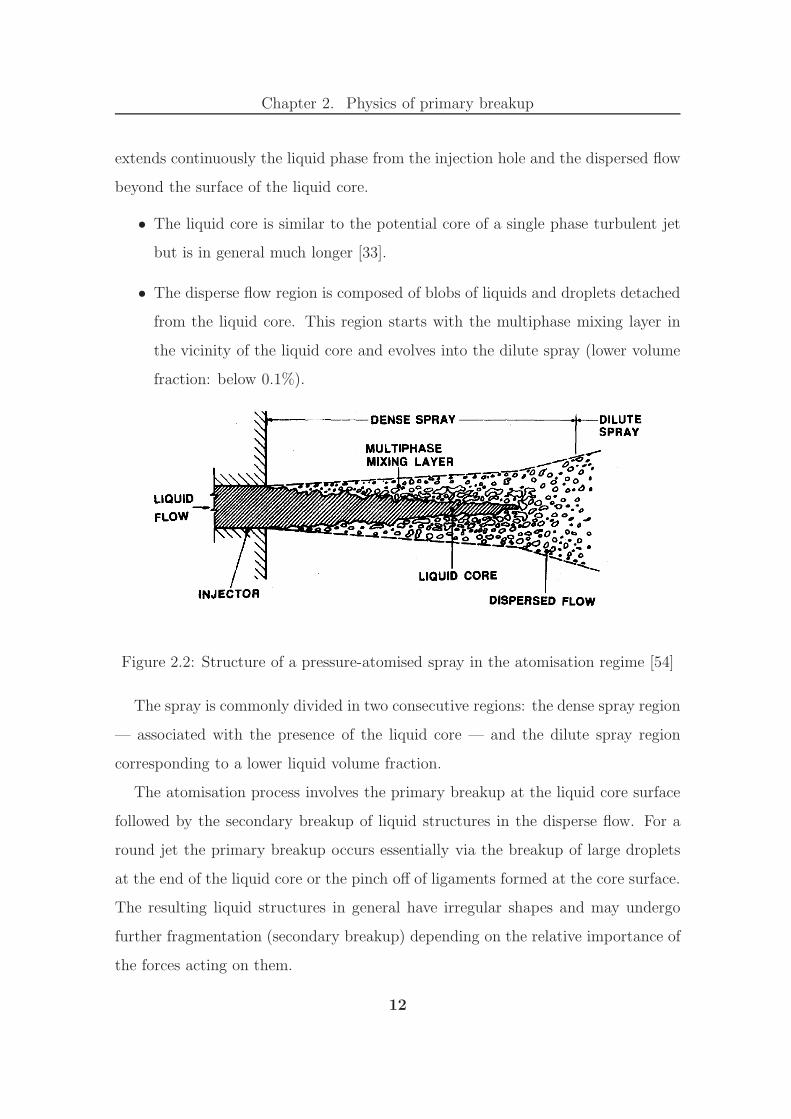
extends continuously the liquid phase from the injection hole and the dispersed flow
beyond the surface of the liquid core.
• The liquid core is similar to the potential core of a single phase turbulent jet
but is in general much longer [33].
• The disperse flow region is composed of blobs of liquids and droplets detached
from the liquid core. This region starts with the multiphase mixing layer in
the vicinity of the liquid core and evolves into the dilute spray (lower volume
fraction: below 0.1%).
Figure 2.2: Structure of a pressure-atomised spray in the atomisation regime [54]
The spray is commonly divided in two consecutive regions: the dense spray region
— associated with the presence of the liquid core — and the dilute spray region
corresponding to a lower liquid volume fraction.
The atomisation process involves the primary breakup at the liquid core surface
followed by the secondary breakup of liquid structures in the disperse flow. For a
round jet the primary breakup occurs essentially via the breakup of large droplets
at the end of the liquid core or the pinch off of ligaments formed at the core surface.
The resulting liquid structures in general have irregular shapes and may undergo
further fragmentation (secondary breakup) depending on the relative importance of
the forces acting on them.
12
Chapter 2. Physics of primary breakup
2.3.3 Properties of round jet sprays
The properties of such sprays are influenced by a wide range of parameters such
as the nozzle exit flow conditions, occurrence of cavitation in the nozzle, velocity
profiles, turbulence level in both phases, etc . . . In particular, Faeth et al. observed
that the droplet size after the primary breakup and the mixing rate between the two
phases are very dependent on the phase density ratio, the flow development and the
turbulence level at the nozzle exit [54].
From the analysis of experimental data, Faeth et al. also reported that the droplet
sizes, after the primary breakup as well as after the secondary breakup, follow the
universal root-normal distribution characterised by a single moment: MMD/SMD
= 1.2 due to Simmons [233].
2.3.4 Ligament formation
As illustrated in the four different regimes of round jet breakup, the behaviour of
the jet depends strongly upon the relative liquid-gas velocity. Whereas the whole
liquid column is deformed at low relative velocities, leading to the formation of bags
and rims; the liquid jet is merely peeled off at its surface at higher relative velocities
resulting in the formation of ligaments. The latter regime being more relevant to
aero-engine injection, the ligament formation is detailed below.
Fuster et al. [65] summarise the action of primary breakup at high velocities by
two phenomena: the detachment of small ligaments (and droplets) from the jet and
further downstream the breakup of large droplets due to the growth of large scale
instabilities on the jet surface.
While linear stability analysis and weakly non-linear theories — reviewed in [52]
— describe with success the growth of longitudinal (Kelvin-Helmoltz) instabilities
along the jet, the formation of ligaments is not well understood. Two mechanisms
have been proposed to explain the origin of ligaments:
• Faeth et al. [54] hypothesised that if a sufficient level of turbulence is attained
13

Chapter 2. Physics of primary breakup
in the liquid phase, upstream of the nozzle, it could deform the interface and
lead to the breakup. The ligament would therefore be formed thanks to a
turbulent eddy with sufficient energy to overcome surface tension.
• Marmottant and Villermaux [146] modelled the flow around the jet interface
by a two-phase mixing layer. In this framework, they demonstrated (using
stability analysis) that a sufficient relative velocity between phases leads to
the growth of a series of instabilities on the jet surface and then results in the
formation and the breakup of ligaments.
Interface deformation by turbulence in the liquid phase The hypothesis
of Faeth et al. [54] resulted from the analysis of the experimental work of [92, 93,
142, 206, 207, 274–277] on round jets breaking up in a quiescent gas. In particular,
they noted that:
• The droplet sizes after primary breakup are strongly related to both the level
of flow development and the intensity of the turbulence at the nozzle exit,
• The breakup is associated with the presence of a turbulent boundary layer in
the liquid phase, at the nozzle outlet,
• The liquid phase properties govern almost entirely the primary breakup prop-
erties for large density ratios (> 500),
• The onset of turbulent primary breakup is strongly related to the laminar-
turbulent transition in the injector passage.
In addition, basing their analysis on time scale considerations, Faeth et al. argue
that the droplets produced near the nozzle exit (i.e. at the onset of the primary
breakup) are the smallest that can be formed [54]. The size of the smallest drop is
then given by the size of the “critical turbulent eddy” which has just enough kinetic
energy to provide the surface energy to form a drop. When the “critical turbulent
14

Chapter 2. Physics of primary breakup
eddy” reaches the limit of the inertial range of the turbulence, the smallest droplets
are then comparable to the Kolmogorov micro length scale.
Ligament formation through a series of instabilities The assisted at-
omization of a liquid jet comes with the formation of ligaments at the jet surface
(regardless of the geometry) conditioned upon sufficient shear from the gas stream.
These ligaments are regularly spaced in the transverse direction and their number
increases with the gas velocity.
Marmottant and Villermaux describe the ligament formation and breakup in a
sequence of steps for a slow liquid jet sheared by a co-axial gas stream [146]. At
first, the two initially parallel streams of different velocities are subject to the Kelvin-
Helmoltz instability which leads to the formation of axisymmetric undulations on
the liquid interface. The shape of the wave crests become singular as this primary
instability grows and develop into liquid sheets bounded by a rim.
Because the bulk liquid velocity is lower than the travelling speed of the longitu-
dinal undulations at the jet surface, the liquid interface is accelerated perpendicular
to itself, alternatively towards the liquid and the gas phase. When the acceleration
is oriented towards the denser phase, the interface undergoes a Rayleigh-Taylor in-
stability [128, 194, 249] which results in the growth of azimuthal undulations (first
hypothesised by Villermaux and Clanet in [266]). Bremond’s findings corroborate
this hypothesis in [27].
Then, the development of the longitudinal and transverse instabilities leads to the
formation of corrugations at the nodes of their undulations. Initially, these crests
are accelerated with respect to the bulk flow with little deformation until the gas
drag is sufficient to pull them away from the jet and increase their aspect ratio.
Finally, after stretching in the gas stream, these ligaments detach from the liquid
bulk by pinching off their base. With a nearly cylindrical shape, the ligaments are
per se sensitive to the Plateau-Rayleigh instability and thus further fragment into
blobs of liquid.
15

Chapter 2. Physics of primary breakup
Figure 2.3: Photo of the assisted disintegration of a round liquid jet in a co-axial
gas stream [146]
2.4 Liquid sheet breakup
In the planar configuration, the liquid is injected between the two parallel walls of
the injector such that the height of the slit is much smaller than its width in order
to avoid boundary effects.
Although aero-engine injectors usually show an axisymmetric configuration, this
section is of particular relevance to the aeronautical industry as Meyer and Weihs
have demonstrated that the mechanisms are identical for planar and axisymmetric
geometries in the limit of a thin annulus [153]. Meyer and Weihs [153] have also
demonstrated that an annular liquid jet behaves like a full round liquid jet in the
limit of a thick annulus.
A very detailed literature review for the liquid sheet breakup can be found in
[37]. In this section we will simply summarise the main scientific findings in that
field.
16
Chapter 2. Physics of primary breakup
2.4.1 Natural disintegration
The first linear stability calculations for an inviscid 2D liquid sheet in quiescent air
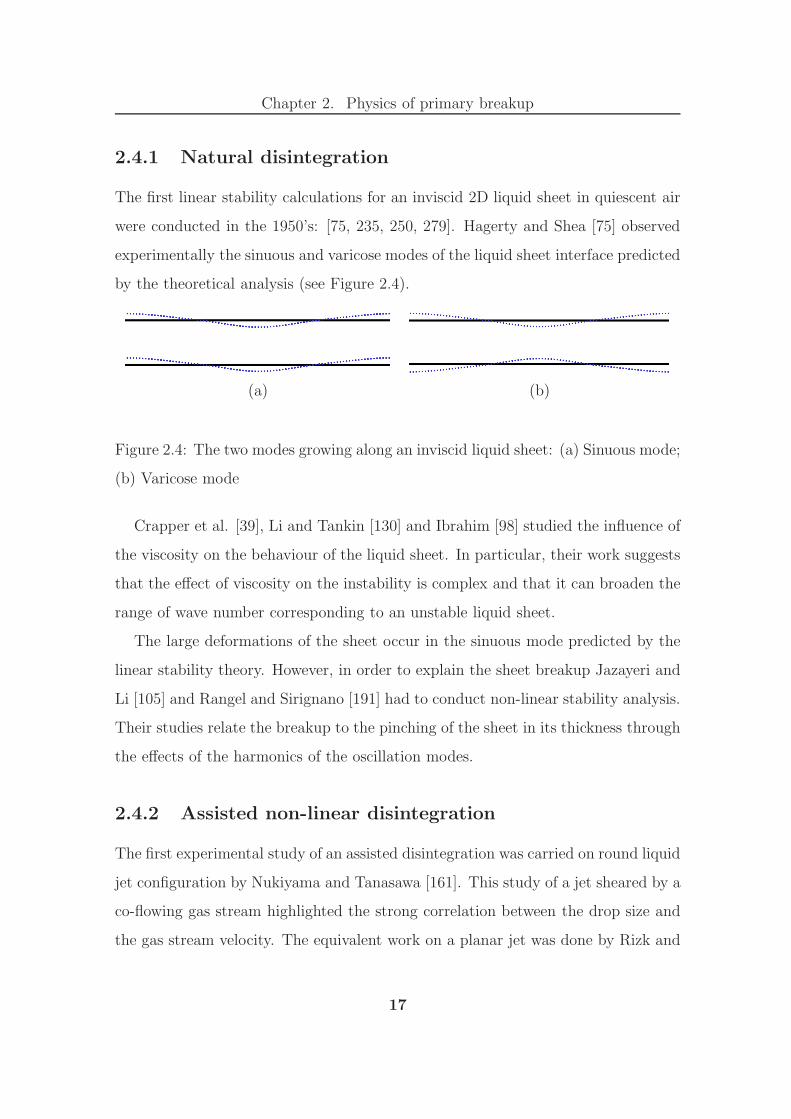
were conducted in the 1950’s: [75, 235, 250, 279]. Hagerty and Shea [75] observed
experimentally the sinuous and varicose modes of the liquid sheet interface predicted
by the theoretical analysis (see Figure 2.4).
(a) (b)
Figure 2.4: The two modes growing along an inviscid liquid sheet: (a) Sinuous mode;
(b) Varicose mode
Crapper et al. [39], Li and Tankin [130] and Ibrahim [98] studied the influence of
the viscosity on the behaviour of the liquid sheet. In particular, their work suggests
that the effect of viscosity on the instability is complex and that it can broaden the
range of wave number corresponding to an unstable liquid sheet.
The large deformations of the sheet occur in the sinuous mode predicted by the
linear stability theory. However, in order to explain the sheet breakup Jazayeri and
Li [105] and Rangel and Sirignano [191] had to conduct non-linear stability analysis.
Their studies relate the breakup to the pinching of the sheet in its thickness through
the effects of the harmonics of the oscillation modes.
2.4.2 Assisted non-linear disintegration
The first experimental study of an assisted disintegration was carried on round liquid
jet configuration by Nukiyama and Tanasawa [161]. This study of a jet sheared by a
co-flowing gas stream highlighted the strong correlation between the drop size and
the gas stream velocity. The equivalent work on a planar jet was done by Rizk and
17
Chapter 2. Physics of primary breakup
Lefebvre [203] and Arai and Hashimoto [8] who also noted, for this configuration,
the important impact of the gas velocity on the SMD and breakup length.
Because the initial deformations of the jet depend strongly on the gas phase, the
presence of a surrounding gas flow changes fundamentally the mechanisms of the
breakup. Cousin and Dumouchel [38] and Barreras [12] produced linear and non-
linear stability analysis specifically for this case and their conclusion was twofold.
First, the same types of mode — sinuous and varicose — grow on the surface of a
liquid sheet sheared by a co-flowing gas; and secondly, the gas and liquid viscosi-
ties and the non-linearity of the interface deformation cannot be neglected in the
analysis.
A major advance on the understanding of the sheet breakup mechanisms was
made in the 1990’s by Stapper et al. [236, 237] and Mansour and Chigier [140,
141]. Noting that the breakup is influenced by a wide variety of parameters, these
authors investigated the breakup regimes obtained for a broad range of conditions.
Specifically, their studies consider the influence of the following physical variables:
surface tension, viscosity, thickness of the sheet (200µm to 1mm), velocities in the
liquid (1 to 5ms−1) and the gas (15 to 60ms−1).
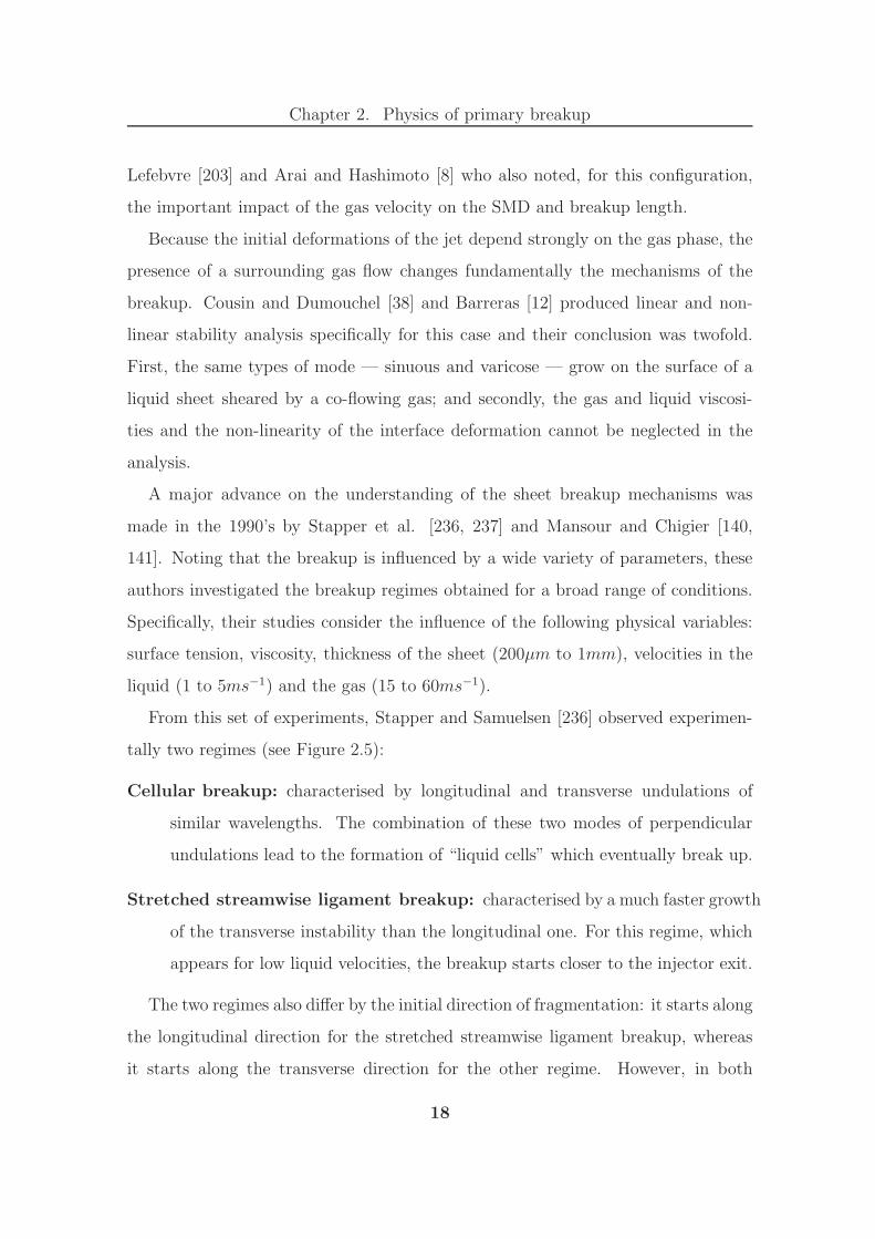
From this set of experiments, Stapper and Samuelsen [236] observed experimen-
tally two regimes (see Figure 2.5):
Cellular breakup: characterised by longitudinal and transverse undulations of
similar wavelengths. The combination of these two modes of perpendicular
undulations lead to the formation of “liquid cells” which eventually break up.
Stretched streamwise ligament breakup: characterised by a much faster growth
of the transverse instability than the longitudinal one. For this regime, which
appears for low liquid velocities, the breakup starts closer to the injector exit.
The two regimes also differ by the initial direction of fragmentation: it starts along
the longitudinal direction for the stretched streamwise ligament breakup, whereas
it starts along the transverse direction for the other regime. However, in both
18

Chapter 2. Physics of primary breakup
instances, the transverse instability and the co-flowing shearing gas stream leads
to the formation of ligaments at the top of the crests. Mansour and Chigier [140]
identified a third breakup regime apparent at low liquid velocities by plotting the
fundamental mode of the sheet undulations against the liquid exit velocity. However,
this regime was less studied by the authors.
Experimental studies [136, 140, 237] suggested that the stretched streamwise
ligament breakup provides the best atomisation (large deformation of the sheet,
wide spray angle and smaller droplets). The mechanism of this regime can be
summarised in a series of steps. At first the liquid sheet undergo a Kelvin-Helmoltz
instability, leading to the quick growth of the sinuous mode, which results in the
flapping of the sheet. This growth carries all along the jet atomisation leading to
the scattered shedding of droplets. Downstream of the zone of flapping, transverse
undulations appear (see [266]) leading to the formation of streamwise ligaments
under aerodynamic forces. These ligaments then stretch and eventually fragment
into relatively large droplets [237]. The liquid blobs produced eventually undergo a
secondary breakup.
(a) (b)
Figure 2.5: The two sheet breakup regimes observed by Stapper and Samuelsen
[236]: (a) Cellular breakup; (b) Stretched streamwise ligament breakup
In the 2000’s various authors have tackled the parameterisation of the primary
19

Chapter 2. Physics of primary breakup
breakup. In particular, Lozano et al. [136] revealed the linear dependence of the
frequency of oscillation against the gas velocity and noted the insignificance of the
influence of the liquid velocity. Lozano et al. [136] and Carentz [31] have also
shown that the reduced oscillation of the global undulation is strongly related to
the momentum ratio gas/liquid. Taking into account the work of Siegler et al.
[232] on the influence of the sheet thickness, the flapping of the sheet has been
characterised by two non-dimensional numbers: the momentum flux ratio and the
reduced frequency of the oscillation. Using the subscripts gas and liq to refer to the
gas and liquid phases respectively, the momentum flux ratio M reads:
M =ρgasU
2gas
ρliqU2liq
(2.2)
The effect of the gas boundary layer on the onset of the sinuous instability has
been studied through both stability analysis and experimental approach. Raynal
[195], Lozano et al. [135, 136] and Marmottant and Villermaux [145, 146] have
concluded that the thickness of the viscous layer — originating from the friction
on the injector walls — has a major influence on the scales of instability. More
precisely, these studies suggest that the thickening of the boundary layer reduces
the growth rate and the wave number for which the growth rate is maximum.
This literature review has highlighted the complexity of the atomisation process. It
has also pointed out that the scientific community has a relatively limited under-
standing of the phenomenon.
As the experimental approach struggles to provide useful insight in the physi-
cal mechanisms controlling the primary breakup, research studies suggest that a
significant breakthrough could be achieved with the numerical approach.
This chapter identifies and describes the fundamental features of the primary
breakup. These will be critical in the choice of a suitable numerical method to
simulate the phenomenon.
20
Chapter 3
Numerical modelling of
multiphase flows
The numerical tool provides a framework to calculate the solutions of the Navier-
Stokes equations in the idealised representation of an experimental setup. Therefore,
it constitutes an intermediate step between the analytical and the experimental
approaches. The realism of these numerical experiments can be raised up to a
certain limit, depending on the complexity of the problem. More precisely, the level
of idealisation concerns principally: the dimensionality of the domain (2D vs. 3D),
the complexity of the physical models embedded in the equations (e.g. description
of the interface for multiphase flows), the level of sophistication of the boundary
conditions (e.g. velocity profiles) and the treatment of the turbulence.
After detailing the mathematical formulation of the problem in Section 3.1, this
chapter presents the numerical methods available to capture the physics of two-
phase flows. In particular, the modelling strategies handling the smallest scales of
the flow field are considered in Section 3.2, the interface description techniques are
reviewed in Section 3.3 and the means of treating the singularities associated with
the presence of the interface are presented in Section 3.4.
21
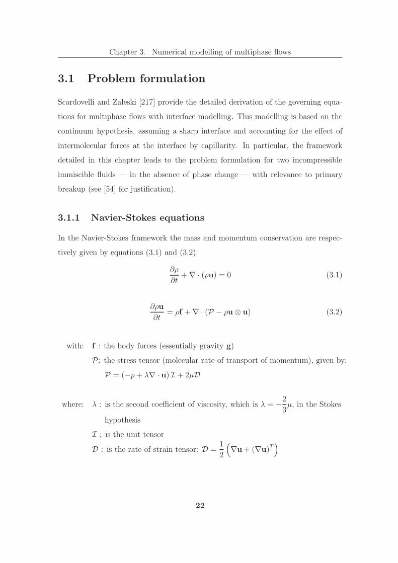
Chapter 3. Numerical modelling of multiphase flows
3.1 Problem formulation
Scardovelli and Zaleski [217] provide the detailed derivation of the governing equa-
tions for multiphase flows with interface modelling. This modelling is based on the
continuum hypothesis, assuming a sharp interface and accounting for the effect of
intermolecular forces at the interface by capillarity. In particular, the framework
detailed in this chapter leads to the problem formulation for two incompressible
immiscible fluids — in the absence of phase change — with relevance to primary
breakup (see [54] for justification).
3.1.1 Navier-Stokes equations
In the Navier-Stokes framework the mass and momentum conservation are respec-
tively given by equations (3.1) and (3.2):
∂ρ
∂t+ ∇ · (ρu) = 0 (3.1)
∂ρu
∂t= ρf + ∇ · (P − ρu ⊗ u) (3.2)
with: f : the body forces (essentially gravity g)
P: the stress tensor (molecular rate of transport of momentum), given by:
P = (−p+ λ∇ · u) I + 2µD
where: λ : is the second coefficient of viscosity, which is λ = −2
3µ, in the Stokes
hypothesis
I : is the unit tensor
D : is the rate-of-strain tensor: D =1
2
(∇u + (∇u)T
)
22

Chapter 3. Numerical modelling of multiphase flows
3.1.2 Incompressible flows
It is generally assumed that both the liquid and the gas are incompressible in multi-
phase flow modelling which supposes that the speed of the flow is much lower than
the speed of sound (Ma ≪ 1) everywhere in the domain considered. This hypoth-
esis leads to equations (3.3) and (3.4) for the mass and momentum conservation
respectively:
∇ · u = 0 (3.3)
ρ
(∂u
∂t+ u · ∇u
)= −∇p + ∇ · (2µD) + ρf (3.4)
This assumption is generally true for most breakup conditions; however Tanguy
[246] has questioned its validity in the case of pockets of gas trapped by ligaments
merging back with the liquid core. Besides, various compressible formulations of
the Navier-Stokes equations have been derived for multiphase flow modelling (see
[154, 160, 190, 212]).
3.1.3 Fluid mechanics with interfaces
The whole multiphase domain can be divided into sub-domains filled with the dif-
ferent phases. In each sub-domain, the Navier-Stokes equations hold, whereas on
the interfaces the connection between domains is simply obtained through mass
and momentum conservation. This leads to the formulation of jump conditions for
quantities discontinuous across the interface.
Material properties Introducing [ ]Γ : the jump condition operator across the
interface Γ , the jump in material properties is expressed by:
[ρ]Γ = ρliq − ρgas (3.5)
23

Chapter 3. Numerical modelling of multiphase flows
[µ]Γ = µliq − µgas (3.6)
Mass conservation Without phase change, the continuity of fluid velocity
leads to equations (3.7) and (3.8) in the jump notation:
uliq = ugas (3.7)
[u]Γ = 0 (3.8)
Introducing n: the unit normal to the interface, equation (3.8) implies that the
velocity of the interface is the normal velocity, V , and that it does not change across
the interface:
V = uliq · n = ugas · n (3.9)
NB: In the case of phase change, the normal velocity is given by u′ = u · n − V ,
in the frame of reference moving with the interface. Applying the Rankine-
Hugoniot equation, the conservation of mass leads to: ρliqu′liq = ρgasu
′gas = q,
where q is the mass transfer from one phase to the other. Expressed in the
general frame of reference, it reads: ρliq (uliq · n − V ) = ρgas (ugas · n− V ) = q
The continuity of normal velocities across the interface, obtained for q = 0 , is
a consequence of mass conservation whereas the continuity of tangential velocities
(ut = u− (u · n) n) is an assumption.
Momentum conservation The momentum conservation across the interface
can be written as the following jump condition:
[−pI + 2µD]Γ · n = σκn + ∇Γσ (3.10)
which can be split into normal and tangential stress conditions (noting : t(k) two
independent vectors tangent to Γ):
[−p + 2µn · D · n]Γ = σκ (3.11)
24

Chapter 3. Numerical modelling of multiphase flows
[µt(k) · D · n
]Γ
= t(k) · ∇Γσ (3.12)
The surface tension term acts as a force concentrated on the interface. The following
notations have been introduced:
• ∇Γ the gradient operator restricted to the surface.
• σ is the surface tension. In general, σ is assumed constant along the interface
(∇Γσ = 0) which results in a continuous tangential stress across the interface:[µt(k) · D · n
]Γ
= 0
• κ is the curvature of the interface, defined by:
κ = −∇Γ · n (3.13)
3.1.4 Whole domain formulation
A whole domain formulation can be developed as an alternative to the “jump condi-
tion form” of the previous section. In this formulation the Navier-Stokes equations
are expressed over the whole multiphase domain and the interface is accounted for
through singular source terms. These singular terms balance each other thanks to
the jump conditions.
The presence of the interface does not involve source terms for the mass conser-
vation. Consequently, the continuity equation remains unchanged:
∇ · u = 0 (3.14)
The momentum balance is given by:
ρ
(∂u
∂t+ u · ∇u
)= −∇p + ∇ · (2µD) + ρf + fcap (3.15)
The source term fcap = σκδΓn + (∇Γσ) δΓ (where δΓ denotes a distribution concen-
trated on the interface) has been added to represent the singular capillary forces.
25

Chapter 3. Numerical modelling of multiphase flows
The jump condition on stress (3.10) allows the balancing of the singularities poten-
tially appearing in the terms: ∇p , ∇. (2µD) and fcap of the momentum equation.
3.1.5 Conservative form
The conservative formulation of the Navier-Stokes equations requires the expression
of the capillary effects by a tensor:
Tσ = −σ (I − n⊗ n) δΓ (3.16)
Lafaurie et al. [119] showed that the capillary forces could be written as: σκδΓn +
(∇Γσ) δΓ = −∇ · Tσ. In the absence of body force, this leads to the following
conservative form of the momentum balance:
∂ρu
∂t= −∇ · (pI + ρu ⊗ u + Tσ − 2µD) (3.17)
3.2 Numerical framework
The numerical frameworks suitable to model the primary breakup involve interface
description techniques. They can be split into two main types: direct numerical
simulation (DNS) and large eddy simulation (LES).
3.2.1 Direct numerical simulation of atomisation
The challenges of modelling atomisation
One of the main difficulties of modelling the whole atomisation process comes from
the breadth of length and time scales involved in the governing physical phenomena.
This requirement is particularly challenging for DNS studies aiming to reduce the
uncertainty in the physics by resolving all the length and time scales of the flow. In
addition to the Kolmogorov length scale η — the smallest scale in turbulent flows —
multiphase flows require the resolution of the smallest liquid structure: ζ . However,
26

Chapter 3. Numerical modelling of multiphase flows
with the change in the topology of the interface, this length scale tends to zero
and therefore cannot be resolved using DNS and a certain level of modelling has to
be introduced to handle this issue. With these models, a proper simulation of the
atomisation process would associate the smallest liquid structure ζ , to the size of
the smallest droplets produced and, according to Gorokhovski and Herrmann [71],
ζ should be resolved by 2 to 5 grid cells.
The interface thickness — typically a few tenths of nanometres — is orders of
magnitude smaller than the smallest scales captured by the DNS (η, ζ). Therefore,
the primary breakup, like any other multiphase flow problem, involves a disconti-
nuity in material properties across the interface. Most simulations assume constant
density and viscosity in each phase and use a Heaviside function to represent these
quantities in the whole domain. In the case of finite volume schemes, the jump
in material properties is treated by defining the discrete control volume value of a
quantity to be the control volume average. This is the preferred approach for volume
of fluid (VOF) and conservative level set approaches [163] as the volume fraction
is already available for these methods. For finite difference methods, the evolution
of the material properties is described by a smeared out version of the Heaviside
function. Finally, the ghost fluid method (GFM) of Fedkiw et al. [55] avoids any
smearing of the interface by solving the two phases separately and imposing the
jump conditions at the interface. This method requires precise knowledge of the
interface location and is therefore geared towards level set methods.
Even at high “global” We, the capillary effects dominate at small scales and
their role in the breakup process needs to be captured [146]. In addition, surface
tension forces are only active on the (nearly) infinitely thin interface and are therefore
singular. It results that another major complexity of modelling the primary breakup
— and more generally any multiphase flow — is the numerical handling of surface
tension. In order to tackle this issue, Brackbill et al. proposed the continuum
surface force (CSF) method [26] which relies on applying the surface tension as a
volume force on a transition region of finite thickness which represents the interface
27
Chapter 3. Numerical modelling of multiphase flows
between the phases. Besides the jump in material properties, the GFM [55] also
allows for the application of surface tension forces with a pressure jump condition
at the interface. The latter approach avoids spreading the capillary forces and
maintains a sharp interface. However, neither method guarantees the exact balance
between the pressure gradient across the interface and the surface tension forces,
with any interface description technique. This leads to the production of “spurious
currents”: unphysical vortices in the vicinity of the interface.
The turbulence is believed to play a significant role in the atomisation process
both on the primary breakup [54] and on the secondary breakup [7] and [65]. At
the typical conditions of injection in aero-engines the Re is high enough so that
the 3D effects on the primary breakup become significant and 2D simulations of
the atomisation are not relevant. However, depending on the configuration studied,
2D simulations may give some insight into the amplification of instabilities on the
interface before the occurrence of non-linearity [65].
The atomisation process involves, per se, very frequent topology changes with
the merging and the breakup of the interface surfaces. Depending on the technique
employed to describe the interface, some “pinching models” may be require to han-
dle this computational complexity. Implicit interface description methods, such as
VOF and level set, handles the topology changes automatically when two interface
segments enter a computational cell. Although straightforward for these methods,
the topology changes are grid dependent. However, if the grid size is adequately
chosen, the smallest droplet produced is significantly larger than the minimum cell
size and the grid dependency of the droplet size distribution should be negligible.
Explicit interface description methods require the use of numerically expensive al-
gorithms for the breakup or the merging of interfaces but they give the opportunity
to introduce physically based models for the pinching.
Besides, the Courant-Friedrichs-Lewy (CFL) condition must account for the ad-
ditional constraints of the multiphase physics. The restriction on the time step must
therefore account for the effect of gravity, viscosity and surface tension [26, 244]. For
28
Chapter 3. Numerical modelling of multiphase flows
time-dependent flows in a compressible framework, Popinet [182] also noted that the
speed of propagation of sound waves imposes strong restrictions on the time step.
Even though filtering techniques can free the calculation from these restrictions,
Popinet’s studies suggest that the incompressible formulation is more efficient. Be-
sides, since most primary atomisation applications involve low Ma, solving the NS
equation in the variable density incompressible limit can be perceived as a valid
assumption and is the approach chosen in most DNS codes.
Despite all these challenges, some successful DNS of atomisation have been ob-
tained with various interface description techniques. On the Diesel jet configuration,
it is worth mentioning the simulations of Menard et al. [151, 152] with a novel cou-
pled level set-VOF technique (CLSVOF) and Desjardins et al. [47] applying the
conservative level set (CLS) of Olsson and Kreiss [163]. Kim et al. [111] reproduced
the round jet in co-flow of the experiments of Marmottant and Villermaux [146]
by combining the refined level set grid (RLSG) method of Herrmann [85] with the
Lagrangian tracking of the small spherical droplets. The results of these simulations
are further detailed in Section 5.1.
Alternatives to full DNS
DNS is limited on both the maximum We and Re achievable in a simulation. More
precisely, increasing either the We or the Re generally leads to a more complex flow
field with the production of smaller droplets and, in the case of a higher Re, the
generation of smaller vortices. It follows that the resolution required to achieve a
reasonable accuracy is unaffordable for the simulation of the atomisation process in
an aero-engine injector. Consequently, some methods have been developed in order
to work around the difficulty of running brutally DNS on this problem.
In parallel to DNS, some phenomenological models have been proposed in order
to maintain affordable CPU requirements. The existing models are based on the
injection of round blobs from the nozzle and therefore rely on crude simplifications
29
Chapter 3. Numerical modelling of multiphase flows
to represent the primary breakup. However, these models include some of the fun-
damental mechanisms involved in the breakup process such as interface instabilities
[15], jet turbulence [96], cavitation [113] and droplet shedding [278].
The study of atomisers requires modelling upstream of the nozzle (injection chan-
nels, etc) and dealing with a broad range of scales: from the large scale instabilities
of the jet core to the small scale ligaments. For this purpose, adaptive mesh refine-
ment (AMR) techniques have been developed to scale the simulation with respect
to the relevant quantities (regions of large gradients, large vorticity and small cur-
vature of the interface). These methods allow for accurate simulation of the liquid
atomisation whilst embedding the complex geometry of the injector. Three differ-
ent strategies have been followed for the production of efficiently parallelisable AMR
techniques:
Patch refinement: this approach has been taken by Sussman et al. [241] for their
level set technique. This method involves a hierarchy of nested rectangular
grids, in which each level of refinement is represented by the union of the grid
patches of a given resolution. In order to avoid any numerical artefact of the
AMR, the successive levels of refinement are strictly contained within each
other. Sussman et al. focussed the refinement in the vicinity of the interface
and on regions of high curvature.
Tree-based adaptive solver: this method was developed by Popinet [182, 183]
and combined with a VOF technique. For this technique, the refinement oc-
curs by the equal split of the cell in each of its dimensions, resulting in 4
(respectively 8) leaf cells in 2D (respectively 3D). This type of structure —
called quadtree in 2D and octree in 3D — handles conveniently boundaries
and interfacial flows and is particularly suited for a multigrid implementation.
Popinet combined this technique with the VOF [73] and the marker [185] in-
terface description techniques.
Refined level set grid: this technique is due to Hermann [85, 86]. With this
30

Chapter 3. Numerical modelling of multiphase flows
technique, the solution of the level set equations are solved on a separate,
high resolution Cartesian grid. Hermann [85] combined this method with the
“narrow-band” methodology of Peng et al. [173]: the number of multiphase
equations solved in a computational cell increase with its proximity to the
interface.
Moreover, Herrmann [84] has developed a numerical approach that models the
interface-turbulence coupling by concentrating all the vorticity at the interface which,
therefore, constitutes a vortex sheet of varying strength. The location and motion
of the interface is described using a level set equation which is combined with a La-
grangian formulation to derive an Eulerian transport equation for the vortex sheet
strength. In the resulting simplified system of equations, the relevant physical pro-
cesses occurring at the interface are explicitly described by additional source terms
accounting for the surface tension effects and the stretching of the interface. Presup-
posing that the level-set/vortex sheet method allows studying directly the physical
mechanisms occurring at the interface, Herrmann [84] anticipates to use this frame-
work to develop closure models for LES of turbulent primary breakup. However,
this approach neglects the viscous boundary layer adjacent to the phase interface
which, according to the experimental studies of Marmottant and Villermaux [146],
strongly affect the onset of the breakup.
Finally, LES has been used as a practical alternative to DNS in the simulation
of primary breakup. Most of the simulations of atomisation presented in the litera-
ture are actually “under-resolved DNS”. In particular, the simulations of Diesel jet
atomisation run by Bianchi et al. [18, 19] or Villiers et al. [44] (see Section 5.1)
are based on an LES formulation for a single phase flow and therefore neglect the
interface sub-grid terms. This kind of approach requires grid convergence studies
in order to demonstrate that the non-resolved small scale interfacial terms have no
impact on the solution.
31
Chapter 3. Numerical modelling of multiphase flows
3.2.2 Large eddy simulation
Application to multiphase flow simulation
The geometry of the injection device (size of injection chamber, turbulent struc-
tures developing in the injection channels, wakes behind the separator plates, large
turbulent structures in the combustion chamber) has a significant influence in the
atomisation process and needs to be embedded in the simulation [44, 65]. This
point is further corroborated by the LES simulations of Apte et al. [6, 7] and Riber
et al. [200], involving particle laden flows with secondary breakup models. Their
results — validated against experimental data — highlight the importance of large
scale turbulence and secondary breakup in the resulting droplet size and velocity
distributions. The consideration of such a significant amount of geometry suggests
the use of LES which, according to [44]: “only resolves the eddies large enough to
contain information about the problem geometry”.
The application of LES to the simulation of atomisation implies the description
of the physical mechanisms occurring at the non-resolved scales by ad hoc models
that predict small scale behaviour based on large scale parameters. Existing sec-
ondary breakup models [167, 168, 196, 197, 248] assume simple geometries for the
liquid structures in order to simplify the description of their interaction with the gas
phase. However, this simplification does not hold in the case of the primary breakup
which has principally been studied numerically via the full description of the inter-
face dynamics. The adoption of an LES methodology that makes this approach
computationally affordable, is based on the ensemble averaging or the spatial filter-
ing of the NS equations and the production of closure models for the sub-grid terms
[28, 29]. However, this task is challenging and besides the effect of surface tension,
very little work has been done to account for the physical mechanisms occurring at
the interface.
In two-phase flows, turbulent energy can be exchanged between phases through
the interface. Experimental [120] and numerical [62] studies highlight the importance
32
Chapter 3. Numerical modelling of multiphase flows
of the interaction between the turbulence and the interface. In particular, DNS
studies of Fulgosi et al. [62] on the influence of the multiphase topology on the
turbulence showed that a moving interface does not behave as a solid wall: for
a moving interface the level of anisotropy is lower and the turbulence transfer is
increased.
Based on these findings, Labourasse et al. [118] stress the importance of account-
ing for the complex turbulence-interface interactions in LES of two-phase flows. In
particular, the authors highlight the need to produce sub-grid models of the non-
linear transfer of turbulence energy across the interface. In addition, the authors
noted that, in the transfer of turbulent energy between phases, the oscillations of
the interface lead to the modification of the turbulence energy spectrum: absorption
of high frequencies and release of lower frequencies.
Sub-grid scales
Labourasse et al. [118] have conducted an analysis of the turbulence-interface cou-
pling using DNS (VOF and front-tracking methods) in order to study the sub-grid
transfer through the interface. This work focused on the theoretical basis and the
development of the LES formulation (spatial filtering, modelling of the non-resolved
scale contributions) for multiphase flows.
Labourasse et al. identified three categories of closure terms for the LES of
multiphase flows:
The “classical” sub-grid terms: they reproduce the effect of “sub-grid scales
correlations on the resolved flow”. These terms are common with the single
phase studies of turbulent flows and, according to [118], a large amount of
the existing models (reviewed in [211]) can be re-used for LES of multiphase
flows. However, the relative magnitude of these terms may differ from the
classification of Vreman [267, 268] in the vicinity of the interface.
The “pure interfacial” sub-grid terms: they represent the “sub-grid contribu-
33

Chapter 3. Numerical modelling of multiphase flows
tion of the interface characteristics” and can be replaced by a jump condition
at the interface.
The misrepresentation of the “mixed phase volume of fluid”: the cells sur-
rounding the interface contain a mixed phase; their representation by thermo-
dynamical and physical laws leads to a sub-grid error. The study of these
terms was tackled by Duquennoy et al. [51] and Mathieu et al. [149] in their
work on contact lines, but no models are currently available for these effects.
Labourasse et al. [118] discussed the relative magnitude of the various sub-grid
scale terms and the precision of the different filtering techniques. In particular,
the authors noted the better performance of mass-weighted filtering processes and
recommended it for LES of turbulent two-phase flows. In their discussion on the
sub-grid terms, Labourasse et al. reported that the most important ones are related
to inertia as in single-phase flows. However, the modification of these sub-grid effects
near the interface excludes the use of a viscosity assumption to model them. The
correct behaviour for these terms has been reproduced by Boivin et al. [21] with
a “Bardina-like-Smagorinsky-like” model. Besides, in their study, Labourasse et al.
also proposed a model for the capillary-induced term.
3.3 Interface description
3.3.1 Overview
The most popular numerical methods accounting for the presence of the interface
in the computational domain transport the interface either explicitly or implicitly.
More recently hybrid methods have been produced to combine the advantages of
several approaches at the expense of CPU time. A forth group of methods gathering
more unusual techniques such as smoothed particle hydrodynamics (SPH), is also
reviewed in this sub-section under the label “alternative methods”.
34
Chapter 3. Numerical modelling of multiphase flows
Explicit interface description
The changes of topology have to be specified for these methods and it gives the
opportunity to implement some physics-based breakup models. In return, explicit
interface description techniques require the introduction of cumbersome algorithms
to handle merging and breakup of the interface surfaces.
Moving mesh This approach is based on the Lagrangian transport (accord-
ing to the underlying velocity field) of the grid nodes associated with the interface
location. This technique is particularly geared towards the simulation of small am-
plitude motions of the interface and has given accurate results in the case of small
waves and weakly deformed bubbles. In particular, this method has been applied
successfully by Ryskin and Leal [209, 210] to study rising bubbles on a curvilinear
grid and by Magnaudet et al. [138] in the calculation of the flow around spherical
bubbles.
As reported by Hirt et al. [88], in the case of pure Lagrangian transport of the
interface nodes, the mesh can become highly distorted even if frequent regridding
and rezoning are applied during the computation. In order to mitigate this issue,
Hirt developed an arbitrary-Lagrangian-Eulerian (ALE) method [87] for the trans-
port of the grid points. In addition, depending on the flow considered, it can also
be necessary to add or remove grid points. This can be done using the specific
algorithms presented in [61] and [66].
Front tracking The front-tracking method combines the resolution of the flow
properties on a fixed grid with the Lagrangian transport (according to the underlying
velocity field) of a web of massless particles — typically a triangular mesh in 3D —
representing the phase interface. The capillary forces are represented by the CSF
method and interpolated from the interface web to the fixed grid. In line with the
CSF approach, the discontinuities across the interface are smoothed by the use of
delta functions in the transition region between the phases. This technique has
35

Chapter 3. Numerical modelling of multiphase flows
been used principally by Glimm et al. [69] and Univerdi and Tryggvason [261]. In
particular, the latter authors extended it to 3D [260] and applied it to the simulation
of primary breakup [259].
The main advantage of the front-tracking method is the lack of mesh dependency
of the breakup process. In addition, despite not being inherently mass-conservative,
front-tracking methods generally conserve mass with a very high level of accuracy.
Also, the use of high-order polynomial interpolations in conjunction with surface
tracking can lead to very accurate calculations of surface tension [184, 185].
Surface markers allow for simulation of very thin liquid bridges with high accu-
racy; however Scardovelli and Zaleski [217] noted that this is only an advantage in
the absence of surface tension and when the phases have the same densities and
viscosities: “interface transparent to the fluid”. Otherwise, the sub-grid scales of
the velocity and pressure fields will not be resolved without a modification of the
fixed grid.
Moreover, this technique requires the introduction of heavy algorithms to handle
the changes of interface topology. Also, the topological changes and the interface
distortion can lead to the concentration or the stretching of the marker distribution.
There is, therefore, a need to redistribute these particles and re-mesh the interface.
All of these processes need to be done efficiently in the case of the atomisation where
the breakup and merging of the interface occurs frequently.
Implicit interface description
Implicit interface description methods — often referred to as front capturing —
represent the interface through a scalar field advected in a fixed grid. The extension
to 3D formulations of front-capturing techniques is therefore straightforward. In
addition, with such techniques, the changes of the interface topology are handled
automatically as soon as two interface segments enter the same computational cell.
This feature of front-capturing techniques leads to both the inaccurate predic-
36

Chapter 3. Numerical modelling of multiphase flows
tion of the breakup time and the undesirable grid dependency of the pinch off and
reconnection processes. However, Gorokhovski and Herrmann argue that if the grid
is fine enough to capture the fundamental mechanisms of the breakup, the solution
should remain acceptable [71]. Consequently, in order to carry any physical signif-
icance, the front-capturing simulations of the primary breakup have to show grid
independence.
The volume of fluid and level set approaches are the two main implicit interface
description methods. Both techniques are most relevant to the modelling of primary
breakup and a whole section has been dedicated to each method. The phase field
method (PFM) — also describing the interface implicitly on a fixed Eulerian grid
— is briefly outlined below.
Phase field method This numerical method describes two-phase flows from
the Van der Waals-Cahn-Hilliard theory of interfaces. This theory considers the
fluid at a mesoscopic scale intermediary between the macroscopic scale of continuum
mechanics and the molecular scale. It leads to a modelled interface of finite thickness
across which the velocity and density vary continuously. The formulation of the
theory is based on Van der Waals model [264] for the free energy density, f , (3.18),
in which C is the “composition variable” and Ψ is C’s “chemical potential”.
f =1
2α |∇C|2 + βΨ (C) (3.18)
Cahn and Hilliard extended this formulation to time-dependent flows and produced
a modified version of the Navier-Stokes equations embedding a “continuum forcing”
term [30]. In this framework, the surface tension is derived from the energy density
field.
PFM transports the interface using standard advection techniques and is, there-
fore, easy to implement in 3D, even on unstructured grid. Also, because of its
potential for energy dissipation the numerical implementations of this method are
37
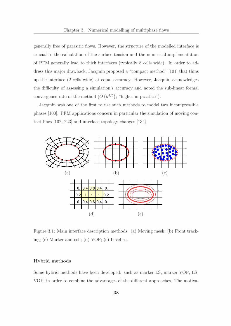
Chapter 3. Numerical modelling of multiphase flows
generally free of parasitic flows. However, the structure of the modelled interface is
crucial to the calculation of the surface tension and the numerical implementation
of PFM generally lead to thick interfaces (typically 8 cells wide). In order to ad-
dress this major drawback, Jacqmin proposed a “compact method” [101] that thins
up the interface (2 cells wide) at equal accuracy. However, Jacqmin acknowledges
the difficulty of assessing a simulation’s accuracy and noted the sub-linear formal
convergence rate of the method (O(h4/5
); “higher in practice”).
Jacqmin was one of the first to use such methods to model two incompressible
phases [100]. PFM applications concern in particular the simulation of moving con-
tact lines [102, 223] and interface topology changes [134].
(a) (b) (c)
(d) (e)
Figure 3.1: Main interface description methods: (a) Moving mesh; (b) Front track-
ing; (c) Marker and cell; (d) VOF; (e) Level set
Hybrid methods
Some hybrid methods have been developed: such as marker-LS, marker-VOF, LS-
VOF, in order to combine the advantages of the different approaches. The motiva-
38

Chapter 3. Numerical modelling of multiphase flows
tion for coupling methods with LS is the advantage of introducing a smooth function
yielding the second-order derivatives needed to calculate the surface tension.
From the point of view of the LS, hybrids methods have been proposed to make
use of better volume conservation properties of auxiliary interface-tracking methods
to correct the LS representation of the interface. In particular, the LS has been
coupled with marker particles — to produce the particle LS (PLS) of Enright et al.
[53] — and with the VOF method that lead to two notable methods: the coupled
LS and VOF (CLSVOF) of Bourlioux [25] (popularised by Sussman and Puckett in
2000 [243]) and the mass-conserving level set method (MCLS) of Van der Pijl et al.
[263]. Both techniques achieve the coupling by defining the volume fraction C, from
the level set function φ as in equation (3.19). Introducing H , the Heaviside function
and Ei, the grid cell considered (3.19) reads:
C (Ei) =1
|Ei|
∫
Ei
H (φ) dEi (3.19)
Hybrids of the VOF and marker particle methods have been produced in order to
improve the interface reconstruction, limit spurious currents and introduce physical
models for the changes in interface topology. In particular, Lopez et al. produced a
2D marker-VOF method [133] to reduce the flotsam (isolated blobs of liquid, artefact
of the VOF interface reconstruction algorithm) and track liquid structures thinner
than the mesh size. The technique adds to the VOF approach some marker particles
at the mid-point of every cell interface segments and reconstructs the interface using
cubic-splines interpolations. Although the addition of marker particles results in a
better control of the interfacial topology changes, the extension of this method to
3D is very difficult.
Alternative methods
Boundary integral (BI) The boundary integral formulation [132] is based on
three assumptions: the viscous forces are negligible compare to the surface tension
39
Chapter 3. Numerical modelling of multiphase flows
forces (inviscid flow and therefore Euler equations), the density of the liquid is
much higher than that of the gas (incompressible liquid in a vacuum) and the flow
— initially irrotational remains irrotational. Under these assumptions, the interface
reduces to a free boundary and can be associated to a vortex sheet [108]. The BI
method simulates the evolution of this vortex sheet by solving an integral equation
along the interface. Despite its severe limitations to simple multiphase flows, this
technique has the advantage to concentrate the mesh on the interface. This method
has been applied to jet breakup [143] and pendant drop [219].
Marker and cell (MAC) The oldest computational methods for tracking an
interface is the “marker and cell” approach of Harlow and Welch [76] formulated in
1965 for free-surface flows where the motion of the light phase is neglected. This
method use both a fixed grid — to simulate the motion of the dense phase in the
region delimited by the free-surface — and massless “volume markers” homoge-
neously distributed in the dense phase and transported with a Lagrangian scheme.
This method, extended to two-phase flows by Daly [40], handles topology changes
automatically and conserves mass reasonably well. However, the MAC approach
requires a large number of markers per grid point in order to capture the inter-
face accurately and avoid high levels of numerical diffusion. Besides, as for surface
marker methods, the flow field may concentrate the particles in places and some
specific algorithms have to be implemented to redistribute the markers.
Lattice Boltzmann method (LBM) The LBM (reviewed in [204, 205]) as-
sociates a continuous fluid to a granular fluid, assuming that the motion of both
types of fluid are similar on a large scale. Instead of solving the Navier-Stokes
equations, this method describe the motion of the particles composing the fluid by
solving the discretised Boltzmann equation combined with a collision model for the
particles. This method emerged from the lattice-gas automata (LGA, [17]) which
is based on a simplified model of the particle dynamics. In the LGA model, the
40
Chapter 3. Numerical modelling of multiphase flows
particles can only move between the nodes of a hexagonal lattice and there can only
be 0 or 1 particle at a certain node moving in a given “lattice direction”. The main
disadvantage of this simple model is the potential rise of statistical noise due to the
Boolean description of the number of particles travelling in a lattice direction. The
LBM solved this problem by using ensemble averages instead of Boolean numbers.
A major drawback common to both LGA and LBM is that these methods describe
the fluid statistically and not necessarily physically.
Smoothed particle hydrodynamics (SPH) Originally developed to solve
problems in astrophysics [68], SPH represents the fluid by a set of particles of prop-
erties distributed over a “smoothing distance” — varying in space and time — using
a kernel function. At a given point, the properties of the fluid are then obtained by
summing the relevant quantity over all the particles in the range of the kernel, so
that the fluid is simulated by the collective properties of the particles. The motion
of the particles is driven by external forces and their mutual interaction. Depending
on their relative distance the particles can either attract (long range) or repel (short
range) each other [155, 156]. The surface tension is then obtained by the repulsion
forces between particles belonging to different phases. With SPH, a large number of
phases can be simulated by introducing as many types of particle and the changes
in interface topology are handled automatically. However, this technique is compu-
tationally intensive and is less attractive than implicit interface description methods
(VOF and LS) for simple two-phase flow situations.
3.3.2 Formulation of the VOF method
This method captures the interface through the transport of the volume fraction,
Ci,j, in the computational domain. The volume fraction — also known as colour
function — represents the volume (respectively the area) occupied by one phase in
a 3D (respectively 2D) computational cell. Consequently, the colour function takes
41

Chapter 3. Numerical modelling of multiphase flows
values between 0 and 1 in the cells cut by the interface and either 0 or 1, depending
on the phase, in the rest of the domain (see consistency equation (3.20)). However,
numerical errors can drive the volume fraction out of this range and some specific
algorithms have to be implemented to avoid non-physical values of Ci,j .
0 ≤ Cni,j ≤ 1 (3.20)
In 1974, DeBar implemented the first VOF method to simulate multiphase flows
with a 2D Eulerian formulation for compressible flows [45]. Nowadays, most imple-
mentations of the VOF method are based on an incompressible formulation of the
Navier-Stokes equations because of the resulting level of simplification. However,
some authors have implemented the VOF technique in the compressible formulation:
see for example [154, 160, 190].
The VOF method involves two stages: the reconstruction of the interface followed
by the transport of the volume fraction. Both of these steps only require the knowl-
edge of the volume fraction and the velocity field (for the latter algorithm) in the
cell considered and its neighbours. This makes the VOF method local and there-
fore highly parallelisable. Also, introducing d, the dimension of the computational
domain and N , the number of cells in one dimension, the advection of the interface
scales as O(Nd−1
)which is small compare to the update of the velocity field.
The major advantage of the VOF method is that it is inherently mass-conservative
(expressed for VOF methods by equation (3.21)). More precisely, in an incompress-
ible formulation, if the technique is implemented with the appropriate numerics
(conservative numerical schemes) it conserves exactly the mass of each phase.
∑
i,j
Cn+1i,j =
∑
i,j
Cni,j (3.21)
The main drawbacks of the VOF method are the uncertainty on the curvature cal-
culation (approximate interface reconstruction) and the diffusion of the interface
42

Chapter 3. Numerical modelling of multiphase flows
(CSF). In the case of under-resolution (radius of curvature of the order of the grid
size), this leads to inaccuracies in the calculation of the capillary forces and the
frequent occurrence in VOF simulations of spurious currents (see Section 3.4). How-
ever, the method remains robust in the limit of very large curvature of the interface
typically encountered during topology changes.
Interface reconstruction algorithm
The determination of the interface curvature — needed for the calculation of the
surface tension — requires the knowledge of the interface shape. For this purpose
the “interface reconstruction” algorithm is implemented in the method and, based
on the volume fractions in a 3× 3 block in 2D (3× 3× 3 block in 3D), provides the
interface location in the cell at the centre of the block.
A broad variety of methods have been developed over the years which can be
gathered in three main groups of algorithms: the simple line interface calculation
(SLIC), the piecewise linear interface calculation (PLIC) and the piecewise parabolic
interface calculation. In the case of a linear interface reconstruction, the various
methods differ on the means to determine the normal n to the segment. Once the
orientation of the surface is known, the approximated interface is completely defined
by the volume fraction in the cell considered.
Novel interface reconstruction methods have been developed in order to reduce the
discontinuities at the cell faces caused by the PLIC representation. In particular,
Manservisi et al. have proposed a method that does this in two steps for a 2D
computational domain [139]. At first, the average curvature is calculated at the cell
considered using a PLIC algorithm with a least square procedure in a 3 × 3 block.
Then, from the two intersections of the fitted circle with the face of the cells, an
internal point is added to better approximate the curvature and conserve the colour
function.
43

Chapter 3. Numerical modelling of multiphase flows
Simple line interface calculation These methods reconstruct the interface
in each cell by a segment aligned with the grid. Being very simple, SLIC algorithms
[89, 159] are usually crude (at best first-order accurate) and lead to the production
of a large amount of flotsam in the transport of the colour function, even in the
case of simple velocity fields (translation, rotation). The original method of Noh
and Woodward [159], calculating the segment location from a 3× 1 block, has been
improved by Chorin [35] — who reconstructs a “stairs-shape interface” by using
a 3 × 3 block — and later by Lafaurie et al. [119]. Because of the geometrical
specificities of an interface reconstructed using SLIC, this method is coupled with
the split advection algorithm.
Piecewise linear interface calculation Amongst the various algorithms pro-
duced for approximating the interface, the most commonly used is the piecewise lin-
ear interface construction (PLIC) method which reconstructs the interface in each
cut cell by a line in 2D (a plane in 3D). Most PLIC algorithms reconstruct the inter-
face as a discontinuous sequence of segments in 2D (polygons in 3D) with “asymp-
totically small discontinuities” [217]. The generation of a continuous interface is
generally perceived as an unnecessary complexity.
Already implemented in the earliest VOF method of DeBar [45], the PLIC method
continues to attract the interest of many authors. In their review of the VOF
algorithms, Pilliod and Puckett assessed the performance of the main PLIC interface
reconstruction schemes against their convergence rates with grid refinement [178].
The test problems used by Pilliod and Puckett involved the typical approximation
of lines, circles, crosses and slotted disks [284].
Based on the principle that a second-order PLIC algorithm reconstructs exactly a
linear interface, Pilliod and Puckett categorise the methods of Puckett and Saltzman
[190] (centre of mass), Parker and Youngs [172] and the central difference algorithm
as first-order accurate whereas the least square volume of fluid interface reconstruc-
tion algorithm (LVIRA) [188] and the efficient LVIRA (ELVIRA) [176] demonstrate
44
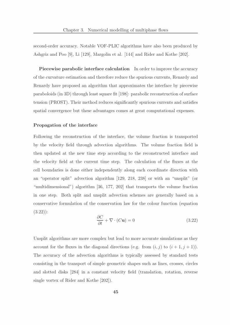
Chapter 3. Numerical modelling of multiphase flows
second-order accuracy. Notable VOF-PLIC algorithms have also been produced by
Ashgriz and Poo [9], Li [129], Margolin et al. [144] and Rider and Kothe [202].
Piecewise parabolic interface calculation In order to improve the accuracy
of the curvature estimation and therefore reduce the spurious currents, Renardy and
Renardy have proposed an algorithm that approximates the interface by piecewise
paraboloids (in 3D) through least square fit [198]: parabolic reconstruction of surface
tension (PROST). Their method reduces significantly spurious currents and satisfies
spatial convergence but these advantages comes at great computational expenses.
Propagation of the interface
Following the reconstruction of the interface, the volume fraction is transported
by the velocity field through advection algorithms. The volume fraction field is
then updated at the new time step according to the reconstructed interface and
the velocity field at the current time step. The calculation of the fluxes at the
cell boundaries is done either independently along each coordinate direction with
an “operator split” advection algorithm [129, 218, 238] or with an “unsplit” (or
“multidimensional”) algorithm [36, 177, 202] that transports the volume fraction
in one step. Both split and unsplit advection schemes are generally based on a
conservative formulation of the conservation law for the colour function (equation
(3.22)):∂C
∂t+ ∇ · (Cu) = 0 (3.22)
Unsplit algorithms are more complex but lead to more accurate simulations as they
account for the fluxes in the diagonal directions (e.g. from (i, j) to (i + 1, j + 1)).
The accuracy of the advection algorithms is typically assessed by standard tests
consisting in the transport of simple geometric shapes such as lines, crosses, circles
and slotted disks [284] in a constant velocity field (translation, rotation, reverse
single vortex of Rider and Kothe [202]).
45

Chapter 3. Numerical modelling of multiphase flows
(a)
(b) (c)
(d) (e)
Figure 3.2: Main interface reconstruction techniques for VOF methods: (a) Ideal
interface; (b) SLIC; (c) Chorin (1980)’s technique; (d) PLIC; (e) FLAIR
The advection of the colour function is both critical, since it drives the mass
conservation properties of a VOF method, and difficult (complexity of “splitting” the
incompressibility condition). In particular, limitations of some existing advection
schemes lead to the violation of the consistency condition (3.20) or the random
production of “wisp” (different from “flotsam”, see [80]) in the bulk of each phase
46
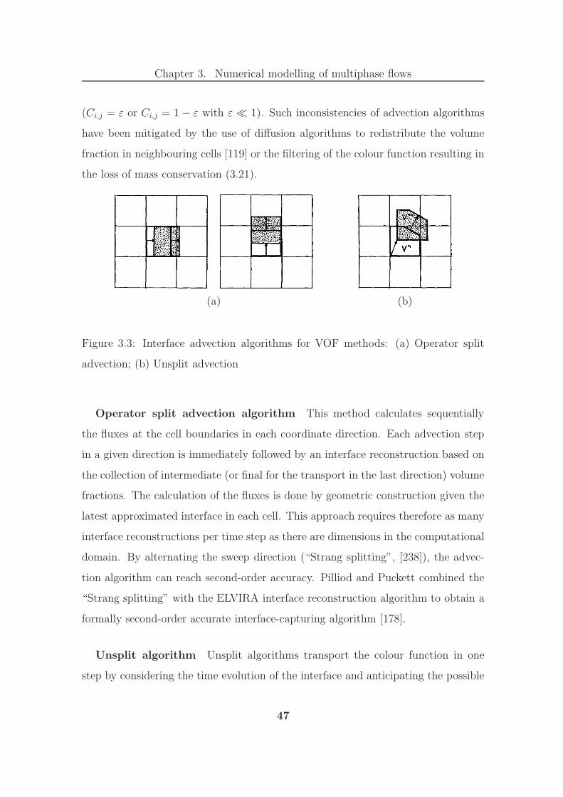
Chapter 3. Numerical modelling of multiphase flows
(Ci,j = ε or Ci,j = 1 − ε with ε ≪ 1). Such inconsistencies of advection algorithms
have been mitigated by the use of diffusion algorithms to redistribute the volume
fraction in neighbouring cells [119] or the filtering of the colour function resulting in
the loss of mass conservation (3.21).
(a) (b)
Figure 3.3: Interface advection algorithms for VOF methods: (a) Operator split
advection; (b) Unsplit advection
Operator split advection algorithm This method calculates sequentially
the fluxes at the cell boundaries in each coordinate direction. Each advection step
in a given direction is immediately followed by an interface reconstruction based on
the collection of intermediate (or final for the transport in the last direction) volume
fractions. The calculation of the fluxes is done by geometric construction given the
latest approximated interface in each cell. This approach requires therefore as many
interface reconstructions per time step as there are dimensions in the computational
domain. By alternating the sweep direction (“Strang splitting”, [238]), the advec-
tion algorithm can reach second-order accuracy. Pilliod and Puckett combined the
“Strang splitting” with the ELVIRA interface reconstruction algorithm to obtain a
formally second-order accurate interface-capturing algorithm [178].
Unsplit algorithm Unsplit algorithms transport the colour function in one
step by considering the time evolution of the interface and anticipating the possible
47
Chapter 3. Numerical modelling of multiphase flows
distribution of heavy fluid (Ci,j = 1) in the cell. Despite requiring only one interface
reconstruction per time step, multidimensional schemes are more complex than op-
erator split algorithms (treatment of fluxes in the diagonal directions) and therefore
harder to implement.
Both first-order [16, 36] and second-order [10, 80, 81, 177, 202] accurate algo-
rithms have been developed over the years. Unsplit algorithms produce better results
than fractional step methods, especially for complicated problems — e.g. unstable
displacement in porous media — where split methods (both first and second-order
accurate) generally lead to the distortion of the interface (“push-pull” or “staircase”
phenomenon, see [16]). In addition, unsplit algorithms resolve better regions of high
variation of the derivatives such as corners of the interface.
3.3.3 Formulation of the level set method
The LS formulation is based on the transport of a continuous function, φ (x, t), in the
computational domain according to the underlying velocity field. In this framework,
the φΓ level set (φΓ = 0 usually) of the function φ represents the interface and φ
takes values below φΓ in one fluid and above φΓ in the other [169, 170, 228]. From
a numerical point of view, a smooth function is desirable and φ is generally taken
as the signed distance function from the interface.
|∇φ| = 1 (3.23)
The background theory for this method was developed by Sethian [224–227] and
the level set technique was originally formulated in [170] to follow fronts propagating
with curvature-dependent speeds (crystal growth, flame propagation). For such
problems, the equations of motion take the form of Hamilton-Jacobi equations with
parabolic right hand sides that account for the curvature effects. This approach has
been implemented in a compressible framework by Mulder et al. [157] to produce a
compressible level set formulation for two-phase flows.
48

Chapter 3. Numerical modelling of multiphase flows
The algorithms developed by Osher and Sethian [170] to follow the propagation
of fronts are based on techniques from hyperbolic conservation laws. The authors
rely upon essentially non-oscillatory (ENO, [77, 79, 230, 231]) numerical schemes
to cope with the formation of large gradients in front propagating problems and
preserve the sharpness of the interface. Such numerics have been further developed
by Liu et al. [131] and later by Jiang and Shu [107] who proposed weighted ENO
(WENO) schemes that offer better precision/robustness trade-offs.
The level set method operates in three steps: at first, the level set function is
defined as the signed distance function (3.23) between any point of the domain and
the interface: φ = 0 on the interface, φ > 0 in one phase, φ < 0 in the other
phase. Then, the scalar φ is transported according to the velocity field (3.24). Once
advected, φ is no longer a signed distance function and a “re-distancing” algorithm
(Section 3.3.3) is applied to maintain φ as a signed distance function to the interface
and prevent φ from becoming irregular.
∂φ
∂t+ u · ∇φ = 0 (3.24)
Like the VOF method, the LS technique handles topology changes naturally. The
main advantage of this method is that it provides the precise front location directly
(no interface reconstruction). This results in the accurate determination of the
interface geometric properties (normal: (3.25) and curvature: (3.26)) and therefore
better calculation of surface tension forces. Besides, the LS formulation is easy to
implement and can be formulated in N dimensions. In particular, since it does not
reconstruct the interface, this method can be extended to 3D more easily than VOF
which requires specific algorithms for this purpose.
n =∇φ|∇φ|
∣∣∣∣∣φ=0
(3.25)
κ = −∇ ·( ∇φ|∇φ|
)∣∣∣∣∣φ=0
(3.26)
49

Chapter 3. Numerical modelling of multiphase flows
The major drawback of this method is that it does not inherently ensure mass
conservation. Although the implementation of an iterative re-initialisation algorithm
[244] partially corrects this issue, the method does not conserve mass accurately.
In order to address this, various methods have emerged: modified re-distancing
algorithms [32, 242], refinement strategies [86] coupling with VOF [150–152, 243,
263], coupling with marker particles [53] or alternative definition of the scalar field
(conservative LS, [163]).
Re-initialisation algorithm
The advection of the scalar φ (3.24) does not ensure that the level set remains a
signed distance function and certain multiphase flow features (high velocity gradi-
ents, interface topology changes) can lead to an irregular level set function (jump at
the interface, spreading). In such instances, the level set function no longer satisfies
the condition (3.23) which is yet required for the precise location of the interface
and the accurate calculation of the its geometric properties ((3.25) and (3.26)). It is
therefore necessary to add a constraint on the transport of φ to maintain the condi-
tion (3.23) without moving the front. This operation, performed by the re-distancing
algorithm, keeps the interface thickness constant.
Originally, re-distancing routines were explicitly searching for the zero level set to
re-initialise φ around the interface. These techniques were computationally expen-
sive [34] and generally lead to severe distortions of the interface. The re-distancing
algorithm of Sussman et al. [244] bypasses the search of the interface by correcting
iteratively the position of the level sets — with respect to the zero level set — such
that (3.23) is satisfied.
In that method, the constraint added on the advection of φ takes the form of a
partial differential equation (3.27) solved on an artificial time step at the end of each
physical time step. Once the artificial steady state reached in the whole domain,
50

Chapter 3. Numerical modelling of multiphase flows
(a) (b)
Figure 3.4: Level sets of a water drop falling under gravity [244]: (a) No re-
initialisation; (b) Re-initialisation
the re-initialisation is complete. Introducing τ , the artificial time step of the re-
initialisation procedure and sign, the sign function mollified around the interface,
this equation reads:∂d
∂τ= sign (φ) (1 − |∇d|) (3.27)
with: d (x, t, τ = 0) = φ (x, t)
This algorithm formally conserves the position of the interface. Indeed, when the
re-initialisation is complete, either |∇φ| = 1 and the property of signed distance
function is recovered or sign (φ) = 0 and x belongs to the interface. At the end of
the iterative process, the level set φ (x, t) is reset to d (x, t, τ = τfinal) in the whole
domain.
The accurate calculation of the interface geometric properties requires the level set
to satisfy (3.23) only in the vicinity of the interface. Since this algorithm starts the
re-initialisation near the interface and propagates outwards in the normal direction,
the re-initialisation of the level set is generally obtained with few iterations per
physical time steps (2 to 3 in practice).
Despite formally maintaining the position of the zero level set, the algorithm of
Sussman et al. still moves the interface slightly in practice. To mitigate this and im-
51

Chapter 3. Numerical modelling of multiphase flows
prove the mass conservation properties of the level set method, Sussman et al. [242]
and Chang et al. [32] have proposed modified versions of the re-distancing algorithm
based on the addition of a constraint (for instance related to the curvature of the
interface) in the solution of (3.27). However, these methods do not systematically
re-distribute the mass appropriately (where it was originally lost) and therefore still
do not satisfy mass conservation exactly.
Conservative level set
Olsson and Kreiss proposed in 2005 the “conservative level set” (CLS) method [163]
based on an alternative definition of level set function. Instead of a signed distance
function, the method transports a hyperbolic tangent function ψ (x, t), that resem-
bles a smeared out liquid volume fraction. As a result, ψ goes smoothly from 0 (in
one phase) to 1 (in the other phase) in a transition region of constant thickness.
The location of interface is then given by the ψΓ = 0.5 level set. Recalling that φ
is the signed distance from the interface and introducing ǫ, a parameter controlling
the thickness of the interface, ψ is defined by:
ψ =1
2
(tanh
(φ
2ǫ
)+ 1
)(3.28)
The level set is transported in two steps: starting with the advection and followed by
the re-initialisation of the level set that maintains the thickness of the transition layer
constant and preserves the smoothness of ψ’s profile. In the case of an incompressible
flow, these equations read:∂ψ
∂t+ ∇ · (uψ) = 0 (3.29)
∂ψ
∂τ+ ∇ · (ψ (1 − ψ) n) = ǫ∇ · (∇ψ) (3.30)
Both steps are implemented with conservative numerical schemes in order to ensure
52
Chapter 3. Numerical modelling of multiphase flows
that ψ is conserved in a divergence free velocity field. However, as the interface has
a finite thickness, this property only leads to the conservation of the volume (in 3D)
bounded by the ψΓ = 0.5 level set in the case of a flat interface [47]. It results that
the volume conservation of the CLS method improves as ǫ decreases for an arbitrary
shape of the interface.
However, a minimum resolution of the level set profile is required for the accurate
calculation of the interface geometric properties ((3.25) and (3.26)) so that Olsson
and Kreiss recommend: ǫ = ∆x/2, where ∆x is the mesh spacing. In the case of the
complex velocity field and topology changes — typical of primary breakup situations
— no satisfactory trade-off can be obtained for ǫ and the inaccurate calculation of n
and κ lead to numerical instabilities. Starting from that method, Desjardins et al.
[47] attempted to mitigate this issue by reconstructing the signed distance function
φ from ψ using Sethian’s fast marching methods [229].
In conclusion, the CLS method reduces the numerical errors accumulated in the
advection of the level set function and, as a result, significantly improves the mass
conservation for the same computational cost as the standard LS technique. Like
hybrid methods, such as PLS [53] or CLSVOF [152, 243, 263], the technique of
Olsson and Kreiss partially solves the mass conservation problem of the level set
method but at a much lower cost. Therefore, the conservative level set method
is a good starting point to develop a numerical method for the simulation of the
atomisation process. It is however necessary to improve the numerical behaviour of
the method in terms of accuracy and stability.
3.4 Treatment of singularities
After presenting the physical origin of the surface tension, this section gives a brief
overview of the principal means of handling singularities numerically. The emphasis
has been placed on the descriptions of the continuum surface force (CSF) [26, 175]
and the ghost fluid method (GFM) [55] as these two techniques are particularly
53
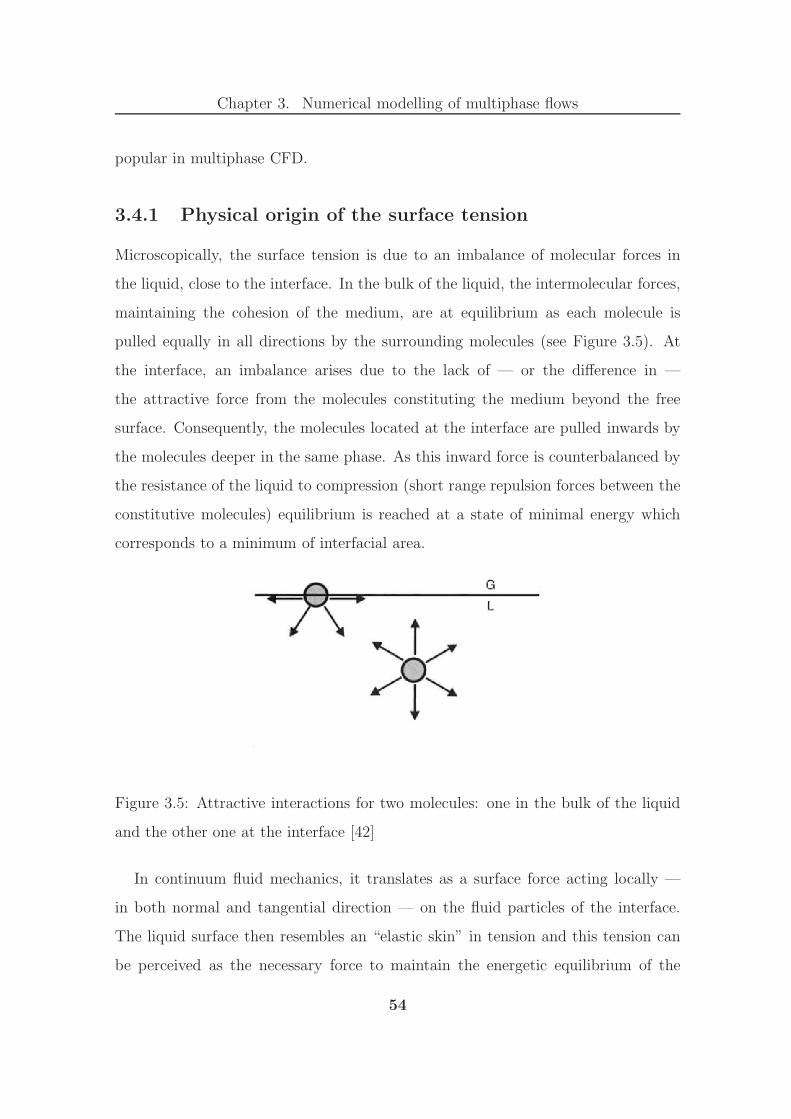
Chapter 3. Numerical modelling of multiphase flows
popular in multiphase CFD.
3.4.1 Physical origin of the surface tension
Microscopically, the surface tension is due to an imbalance of molecular forces in
the liquid, close to the interface. In the bulk of the liquid, the intermolecular forces,
maintaining the cohesion of the medium, are at equilibrium as each molecule is
pulled equally in all directions by the surrounding molecules (see Figure 3.5). At
the interface, an imbalance arises due to the lack of — or the difference in —
the attractive force from the molecules constituting the medium beyond the free
surface. Consequently, the molecules located at the interface are pulled inwards by
the molecules deeper in the same phase. As this inward force is counterbalanced by
the resistance of the liquid to compression (short range repulsion forces between the
constitutive molecules) equilibrium is reached at a state of minimal energy which
corresponds to a minimum of interfacial area.
Figure 3.5: Attractive interactions for two molecules: one in the bulk of the liquid
and the other one at the interface [42]
In continuum fluid mechanics, it translates as a surface force acting locally —
in both normal and tangential direction — on the fluid particles of the interface.
The liquid surface then resembles an “elastic skin” in tension and this tension can
be perceived as the necessary force to maintain the energetic equilibrium of the
54
Chapter 3. Numerical modelling of multiphase flows
molecular cohesion [42]. Upon certain conditions (presence of surfactant, etc . . . ),
the surface tension may vary along the interface which results in the flow from high
surface tension regions to low surface tension regions.
The balance of the normal stresses of two static fluids meeting at an interface of
zero thickness is given by the Young-Laplace equation (3.31). This equation relates
the pressure difference across the interface to the shape of the interface and the
surface tension σ. Introducing the principal radii of curvature R1 and R2 at the
point of the surface considered, (3.31) reads:
∆p = σ
(1
R1+
1
R2
)= σκ (3.31)
3.4.2 Continuum surface force
The CSF method is based on the smoothing of the discontinuous quantities over a
thickened interface (typically 2 to 3 cells wide). It applies the surface tension as
a volume force in this transition region (see Figure 3.6). This technique, generally
associated with the whole domain formulation (see Chapter 3.1), involves introduc-
ing mollified Heaviside and Dirac delta functions in order to make discontinuous
quantities differentiable.
Although robust and easy to implement, this method does not always reproduce
faithfully the physics near the interface, as it diffuses the surface location and the
associated jump conditions. It also relies upon a choice of interface thickness which
drives the trade-off between the accuracy of the interface location and the instability
of the calculations. In addition, both the CSF and the continuum surface stress
(CSS; see last paragraph of this sub-section) formulations of this method tend to
produce non-physical velocities near the interface — the spurious currents — due
to the numerical imbalance between surface tension and pressure gradient.
55

Chapter 3. Numerical modelling of multiphase flows
Figure 3.6: Illustration of the continuum surface force method in 2D [26]
Material properties
Assuming the material properties (density, viscosity) to be constant in each phase
(see Section 3.1), the equation (3.32) gives the value of a given material property, γ,
in the whole computational domain. Using the subscripts gas and liq to refer to the
gas and liquid phases respectively and noting H the Heaviside function, it reads:
γ (x) = γgas +H (x − xΓ) (γliq − γgas) (3.32)
The numerical implementation of (3.32) varies according to the type of scheme
used and the method employed to capture the interface. For interface description
methods that calculate directly the colour function C (VOF, CLSVOF, CLS, see
Section 3.3), the material property considered is then given by:
γ = γgas + C (γliq − γgas) (3.33)
For interface description methods that compute the distance from the interface
φ, i.e. level set methods, the material properties is given by equation (3.34). Intro-
ducing, Hε, the Heaviside function mollified over a distance proportional to ε, (3.34)
reads:
γ = γgas +Hε (φ− φΓ) (γliq − γgas) (3.34)
56
Chapter 3. Numerical modelling of multiphase flows
Surface tension forces
In his analysis of blood flows in the heart, Peskin [175] developed the “immersed
boundary method” to model numerically the surface force exerted by the heart on
the blood. In his framework, the heart wall is modelled by a moving boundary, Γ,
“immersed” in a fixed grid domain. This membrane interacts with the fluid through
a singular surface force, fΓ, approached by a volume force, fΩ, spread on a few cells
surrounding the “immersed boundary”. Introducing the thickness, h, of the region
Ω, surrounding the boundary, then the volume force should give the correct surface
force per unit area when h→ 0:
limh→0
∫
∆Ω
fΩ (x) dΩ =
∫
∆Γ
fΓ (xΓ) dΓ (3.35)
In the integrals of (3.35), the area ∆Γ represents a portion of the interface and ∆Ω is
the small volume of thickness h bounding it. In his formulation, Peskin introduces
an interpolation function, δε, to mollify the Dirac function on a few cells around
the boundary. This convolution kernel satisfies δε → δΓ when ε → 0, where ε is a
parameter of the kernel function, proportional to h. Using the interpolation function
δε, the surface integral of fΓ can be approximated by the following volume integral:∫
Γ
fΓ (xΓ) dΓ ≈∫
Ω
fΓ (x) δε (x − xΓ) dΩ (3.36)
This method has been applied to the numerical handling of surface tension forces by
Brackbill et al. [26] in their “continuum surface force” (CSF). Using the CSF model
and assuming the surface tension uniform (fΓ (x) = σκ (x) n (x)), an expression can
be found for the capillary forces fcap in (3.15). When the colour function is directly
available, fcap is approximated by:
fcap ≈ σκ∇C (3.37)
Similarly, for level set methods the capillary forces are approximated by:
fcap ≈ σκ∇φδε (φ− φΓ) (3.38)
57

Chapter 3. Numerical modelling of multiphase flows
Continuum surface stress
The CSF method implements the surface tension forces from the formulation of the
momentum balance given in (3.15). In (3.15), the surface tension forces are simply
added as a source term on the right hand side of the equation after the calculation
of the interface curvature. Evolving from the CSF, Lafaurie et al. produced the
continuum surface stress (CSS) [119] by expressing the capillary effects as a tensor
(3.16). The CSS then models the surface tension by an added correction in the
momentum stress tensor, based on the local gradient of the volume fraction.
Due to this tensorial formulation of the capillary effects, the CSS is based on a
conservative form of the momentum balance (3.17) and therefore formally conserves
the momentum. Although, the CSS results in stronger spurious currents than CSF,
unlike CSF, this method tends to reduce the magnitude and the spread of these
non-physical velocities under grid refinement [198].
3.4.3 Ghost fluid method
In order to mitigate the limitations of the CSF, Fedkiw et al. [55] proposed a
numerical method that retains a sharp interface, respects the jump conditions and
significantly reduces the spurious currents. The GFM achieves this by extending
continuously the domain of discretisation of each phase into the other phase in a
“ghost region”. This region is typically 3 to 5 cells thick, depending on the movement
of the interface and on the stencil employed.
Although formally in a single fluid formulation, the GFM involves solving the
two phases separately and connecting them through the interfacial jump conditions.
In particular, the surface tension is applied via a pressure jump condition (3.39)
derived from the normal stress conditions (3.11) in the case of an inert interface (no
phase change, no reaction). For a uniform surface tension, the set of jump conditions
linking the two phases reduces to:
[ρ]Γ = ρliq − ρgas (3.5)
58

Chapter 3. Numerical modelling of multiphase flows
[µ]Γ = µliq − µgas (3.6)
[p]Γ = 2 [µ]Γ n · D · n− σκ (3.39)
Once the jump conditions are estimated from the interface characteristics, the
method extends continuously the discontinuous quantities in each “ghost region”
in order to calculate their discrete derivatives. At each time step, a specific algo-
rithm defines these ghost cells so that the boundary conditions for the Navier-Stokes
equations are satisfied. It leads to the simultaneous presence of the two fluids at
every grid point in the two “ghost regions”. In this narrow band around the inter-
face, two sets of mass, momentum and energy equations are solved (using standard
methods), one for the real fluid and the other for the ghost fluid. The appropriate
solution — corresponding to the real fluid at a given location — is then chosen
according to the phase marker of the interface description method (e.g. the sign of
the distance function for LS method).
Figure 3.7: Illustration of the ghost fluid method in 1D [246]
The principle of the method in 1D is illustrated in Figure 3.7 for a given variable
f discontinuous across the interface Γ. Designating Ω− and Ω+ the two domains
separated by Γ, the jump of f , a (xΓ) is defined in (3.40) as a function of xΓ ∈ Γ. In
the LS-GFM framework of Fedkiw et al. [55], a (xΓ) can be expressed as a function
59
Chapter 3. Numerical modelling of multiphase flows
of the distance from the front φ (3.41).
[f ]Γ = f+ − f− = a (xΓ) (3.40)
aΓ =ai |φi+1| + ai+1 |φi|
|φi| + |φi+1|(3.41)
Using these notations, the ghost values f g−i+1 in Ω− and f g+i in Ω+ are defined re-
spectively by (3.42) and (3.43), and the discrete derivative for f is given by (3.44)
in cells crossed by the interface [152].
f g−i+1 = f+i+1 − aΓ (3.42)
f g+i = f−i + aΓ (3.43)
∂f
∂x
∣∣∣∣∣i+ 1
2
=fi+1 − fi
dx− aΓ
dx(3.44)
Fedkiw et al. originally combined the GFM with the level set method which calcu-
lates directly the distance from the interface φ. This interface-capturing method is
ideally associated with the GFM as the interface location and the jump conditions,
essential to the GFM, can be easily derived from φ. As a result, the implementation
of the GFM in a level set solver is wieldy: it reduces to the addition of routines to
define and treat the ghost cells. In addition, the GFM being applicable to a broad
range of jump conditions, the LS-GFM method can be extended to vaporising and
reacting two-phase flows [158]. Early implementation of this method for the simula-
tion of incompressible two-phase flows are reported in [109]. Further developments
of this technique can be found in [90, 91].
60

Chapter 3. Numerical modelling of multiphase flows
3.4.4 Alternative methods
Immersed interface method (IIM) LeVeque and Li have developed this
method to handle jump conditions by applying them directly into the stencil of
discretisation [127]. LeVeque and Li combine these jump conditions with Taylor
series expansions about the interface to derive their difference scheme. Although this
method is precise and reaches second-order accuracy, its algorithms are complex and
difficult to extend to 3D. Successful implementation of the IIM for the simulation
of incompressible Navier-Stokes equations with immersed boundaries are reported
in [126].
“Cut-cell” techniques Popinet and Zaleski developed a 2D front-tracking al-
gorithm (surface markers connected by cubic splines) in order to improve the mod-
elling of surface tension [185]. The authors take advantage of the front-tracking
method to produce a novel technique to represent the surface tension based on the
idea that the interface is a sharp discontinuity. This technique reduces significantly
the spurious currents on the classical test cases (equilibrium bubble, capillary wave
and Rayleigh-Taylor instability) and could be extended to the treatment of other
discontinuous terms across the interface. However, this method relies on complex
geometric considerations and its implementation to 3D is not straightforward.
Parabolic reconstruction of surface tension (PROST) Renardy and Re-
nardy developed a novel technique to handle surface tension by calculating the
curvature of the interface from the least square fit of a quadratic approximation of
the interface [198]. Thanks to a finer approximation of the curvature, this algorithm
dramatically reduces the spurious currents (2 to 3 orders of magnitude lower than
with CSF or CSS) and shows better spatial convergence than both CSF and CSS
methods. However, such improvement in the accuracy of the method comes at a
great computational cost.
61

Chapter 3. Numerical modelling of multiphase flows
3.4.5 Spurious currents
Spurious currents are non-physical velocities — in general vortices — that may
occur in the vicinity of the interface when the interfacial forces are modelled. Most
numerical methods modelling surface tension produce these undesirable features.
These includes front-tracking methods, lattice-Boltzmann methods (in which they
were first observed, see [74]) and CSF methods. In their VOF/PLIC implementation
of the CSF, Lafaurie et al. [119] measured the order of magnitude of these currents
in the case of an equilibrium (static) bubble between two phases of equal density
and viscosity (see Figure 3.8). They reported the following relation:
up ∼ 0.01σ
µ(3.45)
In practice, there are essentially two numerical reasons for the occurrence of spurious
Figure 3.8: Spurious currents in an equilibrium bubble; obtained with the CSF
method [198]
currents. The first one is the discrete imbalance between the surface tension and the
associated pressure gradient across the interface and the second one is the inaccurate
evaluation of the surface curvature.
62
Chapter 3. Numerical modelling of multiphase flows
Francois et al. mitigated the first problem with the “balance-force algorithm”
[59], developed for VOF methods with a CSF model of the interface. This technique
eliminates the spurious currents up to machine accuracy (when the curvature is
exactly known) by using compatible discrete approximations of the pressure and
the volume fraction gradients in the discretised momentum equation. Herrmann
applied the same methodology to correct the numerical imbalance in his refined
level set grid framework [86]. The LS technique have also been combined with the
GFM of Fedkiw et al. [55] and the “sharp-interface method” of Sussman et al. [245]
and both achieved very low magnitudes of spurious currents because they apply the
jump conditions directly on a sharp front.
As surface tension models are becoming more and more accurate, the reduction
of spurious currents relies heavily on the accurate estimation of the curvature. For
VOF methods, the difficulty comes from the discontinuity of the volume fraction
at the interface location and has been addressed by using convolution operations
[273], height-function approaches [83, 183, 240, 245] and high-order interface recon-
struction algorithms [183, 198]. With LS methods, the inaccuracies in curvature
calculations arise from the fact that the interface does not generally pass through
the grid nodes which results in the use of interpolation techniques [137]. Herrmann
reached second-order accuracy with his “interface projected curvature evaluation”
method [86] based on the distribution of the curvature in the whole computational
domain.
In the case of large surface tension and large density ratios, the spurious currents
tend to limit the range of capillary number (Ca) and Laplace number (La) that
can be simulated accurately, in a similar manner that the Re limits the DNS of
homogeneous flows. In particular, above a critical La, corresponding to a large
value of σ, the spurious currents dominate the flow and their growth can lead to the
destruction of the interface. Introducing the characteristic velocity U , and length
63

Chapter 3. Numerical modelling of multiphase flows
L, the Ca and La are defined in equations (3.46) and (3.47) below:
Ca =µU
σ(3.46)
La =σρL
µ2(3.47)
Low values of surface tension can also lead to the destruction of the interface.
This happens for first-order VOF methods, which are unstable in the absence of
surface tension and produce flotsam. Besides, at low Re, a small surface tension
leads to a large Ca which results in the creation of cusps in the interface.
This chapter describes the various options available to study the primary breakup
with the numerical approach. From this literature review, it appears that the simu-
lation of the primary breakup requires an interface-capturing technique to account
for the effect of the geometry on the atomisation process. In particular, the cost-
effective conservative level set method, demonstrated on the primary breakup of
Diesel jets, appears as a good candidate. In addition, due to the breadth of length
and time scales involved in the atomisation process, the LES framework seems nec-
essary to simulate more realistic injection devices.
64
Chapter 4
Multiphase codes
Two different open source multiphase codes have been identified: Gerris [181] and
OpenFOAM [271]. Both codes use VOF to capture the interface and are fairly
well-known and recognised in the field of multiphase CFD.
The two codes are briefly described in Section 4.1 and their comparative perfor-
mance is assessed on typical test cases in Section 4.2. Finally, in Section 4.3, both
numerical capabilities are applied to the simulation of the primary breakup.
4.1 Available codes
4.1.1 OpenFOAM
OpenFOAM was originally developed by Henry Weller at Imperial College in Lon-
don. This code is more a “C++ toolbox” for the numerical solution of continuum
mechanics problems than a dedicated CFD solver for multiphase flows. In that
regard and thanks to the flexibility given by the C++ language, OpenFOAM is
an ideal platform for the customisation and the development of novel CFD meth-
ods. OpenFOAM uses finite-volume numerics on unstructured meshes and therefore
can handle complex geometries easily. In particular, unstructured meshes can be
imported into OpenFOAM from commercial packages (Fluent, Gambit, etc . . . ).
65

Chapter 4. Multiphase codes
Thanks to its flexibility and its versatility, OpenFOAM is already a very popular
open source code used by several companies and universities around the world. The
main issue of the code is its lack of documentation, especially on the implemen-
tation of the boundary conditions. Indeed, the official documentation [165, 166]
details more the general philosophy of the code than it explains how to use it on a
practical problem, as no guidance is given for most of the tutorials. However, some
relevant information can be obtained from the “OpenFOAM message board” and
from reports or presentations produced by OpenFOAM users.
OpenFOAM already embeds several solvers that handle multiphase flows with a
volume of fluid approach. In particular, two different solvers have been identified
as relevant test platforms: the DNS solver interFoam and the LES version of it
lesInterFoam.
4.1.2 Gerris
The CNRS (France), and in particular the group lead by Stephane Zaleski, has
built up a strong capability in the simulation of multiphase flows. Over the years,
this team and its former members (Jie Li, Denis Gueyffier, Stephane Popinet) have
developed several codes (SURFER, Gerris) and perfected the VOF method imple-
mented. Stephane Popinet wrote Gerris in C, using quadtree (octree in 3D) finite
volume discretisation, to solve mainly multiphase flow problems. This code cannot
handle unstructured meshes and treats solid parts as a third phase.
In Gerris, the computational domain is made of 1×1 adjacent boxes, each initially
refined to a given level l with: ∆x = 1/2l. For example a 1 × 2 domain will be
made of two adjacent boxes and a 128 × 256 mesh will be produced by refining the
domain seven times (27 = 128). The mesh adaptation tool allows the user to set the
refinement of each box constituting the domain between two values and according
to a set of chosen criteria.
Although fairly unknown in the past few years, Gerris has recently gained in
66

Chapter 4. Multiphase codes
popularity thanks to the performance of its method. The lack of a user guide is
counterbalanced by detailed online tutorials and the profusion of test cases. Further
information can be obtained through the message board. The main drawback of
this code is the difficulty to develop it, as it was originally written for expert users
to be efficient but not “developer friendly”.
This code gathers state-of-the-art numerical methods for VOF interface descrip-
tion: balanced-force CSF formulation, general height-function interface curvature
[183] and uses tree-based adaptive mesh refinement [182].
4.2 Code validation
4.2.1 Advection algorithm
The assessment of the advection algorithm of a VOF code requires simulating an
interface “transparent” to the flow field. This is achieved by simulating two inviscid
phases of identical density with zero surface tension. In the following sub-section,
L refers to the length of the computational domain and the error field is calculated
by:
∆C = Ct=0i,j − Ct=1
i,j ∀i, j (4.1)
where C is the colour function.
Rotation and translation of a cross The advection of a 2D cross in a solid
body rotation field is a simple test case to assess the performance of the interface
transport algorithm. The computational domain is a square box delimited by the
points (−1;−1) and (1; 1). The cross is made of a 0.6× 0.6 square from which four
smaller 0.2×0.2 squares are subtracted at each corner (see Table 4.1). The cross has
been transported in two different ways with the same velocity field: a pure rotation
of the cross about its centre (0; 0), and a translation along a circular trajectory
(Ctraj = (0; 0), Dtraj = 1). The details of both simulations are summarised in
67

Chapter 4. Multiphase codes
Table 4.1. The end of the simulation is reached after one revolution for t = 1s.
The results of the rotation and the translation are respectively reported in Fig-
ure 4.1 and Figure 4.2 for both codes. OpenFOAM and Gerris perform the rotation
similarly, maintaining the general cross shape. These results compare reasonably
well with the review of the existing advection algorithms performed by Pilliod and
Puckett [178]. As expected the maximum departures from the original shape occur
at the corners. The contours of difference in volume fractions with the original shape
are slightly asymmetrical for OpenFOAM. On the translation problem, Gerris’ ad-
vection algorithm performs equally well and the results present the same pattern as
in the rotation case. However, OpenFOAM breaks down on this problem, showing
surprisingly bad results not only on the corners of the cross but also along its sides
(especially the top of the cross).
Table 4.1: Simulation settings for the advection of a 2D cross
Rotation Translation
Velocity field: ux = −2πy ; uy = 2πx
Grid size: ∆x = L/128
68
Chapter 4. Multiphase codes
On the translation problem, Gerris has also been run with adaptive mesh refine-
ment based on a curvature criterion (see Table 4.4) ideally suited for such problem.
With a level of refinement of 7 (∆x = L/128). The mesh adaptation tool has been
set to refine (resp. coarsen) the mesh up (resp. down) to level 8 (resp. 6) in regions
of high (resp. low) curvature. Not only does this feature significantly improve the
accuracy of the results but — thanks to the coarsening — it also accelerates the
calculation by about 40 %.
The slotted disk of Zalesak Another classic test of the quality of an advection
algorithm is the solid body rotation of a slotted disk. This problem, first set by
Zalesak [284], is particularly difficult as it involves sharp corners and a thin slot
within a solid geometrical shape. Depending on the quality of the scheme, this
latter feature may disappear resulting in a modified topology. The computational
domain is a square box delimited by the points (−1;−1) and (1; 1). The shape is
made of a disk of diameter 0.6, centred on (0; 0.5) from which a vertical rectangle
of 0.1 × 0.5 is subtracted (see Table 4.2). The slotted disk is then translated along
a circular trajectory (Ctraj = (0; 0), Dtraj = 1) like the cross in the previous case.
The simulation settings for this problem are given in Table 4.2. The end of the
simulation is reached after one revolution for t = 1s.
The results, summarised in Figure 4.3, show that both codes maintain the topol-
ogy of the slotted disk. However, as in the previous test case, Gerris significantly
outperforms OpenFOAM. In particular, OpenFOAM produces unexpected wiggles
on the top of the disk. Like in the case of the advection of the 2D cross the worst
results are obtained on the top of the translated geometry: the region that travels
the most.
Disk in a deformation field This test assesses the ability of the code to
represent thin ligaments on coarse grids and to avoid the generation of flotsam. In
the first half of the simulation (up to t = 3s) a 0.3 disk, centred on (0.5; 0.75) in
69
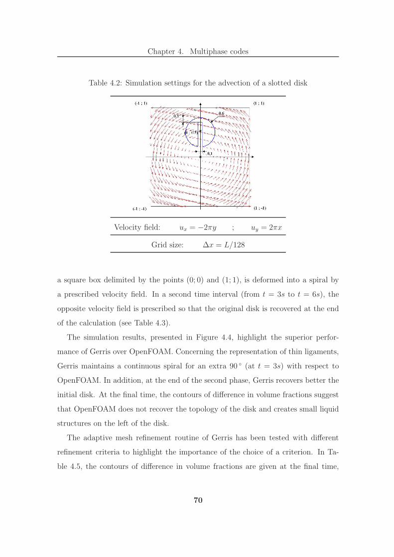
Chapter 4. Multiphase codes
Table 4.2: Simulation settings for the advection of a slotted disk
Velocity field: ux = −2πy ; uy = 2πx
Grid size: ∆x = L/128
a square box delimited by the points (0; 0) and (1; 1), is deformed into a spiral by
a prescribed velocity field. In a second time interval (from t = 3s to t = 6s), the
opposite velocity field is prescribed so that the original disk is recovered at the end
of the calculation (see Table 4.3).
The simulation results, presented in Figure 4.4, highlight the superior perfor-
mance of Gerris over OpenFOAM. Concerning the representation of thin ligaments,
Gerris maintains a continuous spiral for an extra 90 (at t = 3s) with respect to
OpenFOAM. In addition, at the end of the second phase, Gerris recovers better the
initial disk. At the final time, the contours of difference in volume fractions suggest
that OpenFOAM does not recover the topology of the disk and creates small liquid
structures on the left of the disk.
The adaptive mesh refinement routine of Gerris has been tested with different
refinement criteria to highlight the importance of the choice of a criterion. In Ta-
ble 4.5, the contours of difference in volume fractions are given at the final time,
70

Chapter 4. Multiphase codes
Table 4.3: Simulation settings for the disk in a deformation field
Velocity field for t ∈ [0; 3] (s): ux = −∂ψ∂y
; uy = ∂ψ∂x
Velocity field for t ∈ [3; 6] (s): ux = ∂ψ∂y
; uy = −∂ψ∂x
With: ψ = 1π
sin2 (πx) sin2 (πy)
Grid size: ∆x = L/128
t = 6s, for the simulations without AMR, with adaptation based on the gradient of
colour function (C) and with adaptation based on the curvature. Apart from the
criterion, the adaptation settings are the same as for the translation of the cross.
The results clearly show that for an interface with a lower curvature (except at the
tip of the spiral), the adaptation based on the gradient of the color function performs
better. Logically, the higher number of cells resulting from this adaptation criterion
leads to a longer simulation time.
71
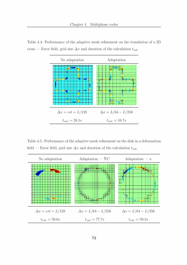
Chapter 4. Multiphase codes
Table 4.4: Performance of the adaptive mesh refinement on the translation of a 2D
cross — Error field, grid size ∆x and duration of the calculation tcalc
No adaptation Adaptation
∆x = cst = L/128 ∆x = L/64 − L/256
tcalc = 28.1s tcalc = 16.7s
Table 4.5: Performance of the adaptive mesh refinement on the disk in a deformation
field — Error field, grid size ∆x and duration of the calculation tcalc
No adaptation Adaptation — ∇C Adaptation — κ
∆x = cst = L/128 ∆x = L/64 − L/256 ∆x = L/64 − L/256
tcalc = 50.6s tcalc = 77.7s tcalc = 59.2s
72

Chapter 4. Multiphase codes
OpenFOAM Gerris
Interface at t = 1s
Error field
Figure 4.1: Performance of the advection algorithms on the rotation of a 2D cross
— Comparison OpenFOAM vs. Gerris
73
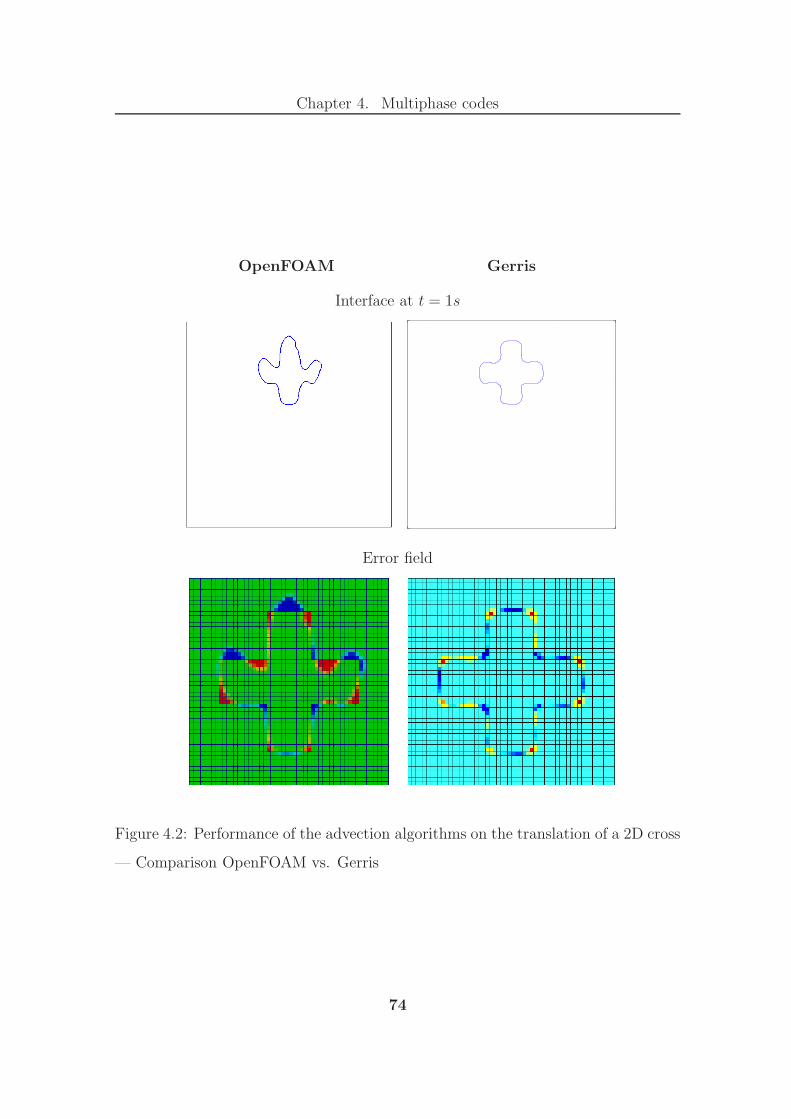
Chapter 4. Multiphase codes
OpenFOAM Gerris
Interface at t = 1s
Error field
Figure 4.2: Performance of the advection algorithms on the translation of a 2D cross
— Comparison OpenFOAM vs. Gerris
74

Chapter 4. Multiphase codes
OpenFOAM Gerris
Interface at t = 1s
Error field
Figure 4.3: Performance of the advection algorithms on the slotted disk of Zalesak
— Comparison OpenFOAM vs. Gerris
75

Chapter 4. Multiphase codes
OpenFOAM Gerris
Interface at t = 3s
Interface at t = 6s
Error field
Figure 4.4: Performance of the advection algorithms on a disk in a deformation field
— Comparison OpenFOAM vs. Gerris
76

Chapter 4. Multiphase codes
4.2.2 Basic two-phase flows
Rayleigh-Taylor instability This test case is usually used to demonstrate
the numerical convergence of an interface description method. The Rayleigh-Taylor
instability is also used to study the capability of code to capture thin ligaments in
the presence of surface tension and with a significant density ratio between phases.
Simulations of the Rayleigh-Taylor instability have been carried out with various
interface description methods by many authors in both 2D and 3D [133, 185, 189,
260].
The problem is set in a rectangular box (free-slip boundary conditions imposed
on all four walls) of 1m×4m in which two phases of different densities and identical
viscosities equally share the domain. The heavier fluid occupies the top half of
the domain and is initially separated from the light fluid by a cosine interface of
maximum amplitude 5×10⁻²m. Under buoyancy effects and because of the original
perturbation of the interface, the heavier fluid falls into the light one. The details
of the simulation settings are given in Table 4.6.
Table 4.6: Simulation settings for the Rayleigh-Taylor instability
Initial interface position: y = −0.05 cos (2πx)
Density: ρ1 = 1.255kgm−3 ρ2 = 0.1694kgm−3
Viscosity: µ1 = µ2 = 3.13 × 10⁻³kgm−1s−1
Surface tension: σ = 1 × 10⁻²Nm−1
Gravity: g = 9.81ms−2
Mesh size: 128 × 512
The problem, as formulated in [189] has been simulated with OpenFOAM and
Gerris. The results of both codes, presented in Figure 4.5, compares satisfactorily
with the calculations presented in [133, 185, 189]. However, as demonstrated in the
77
Chapter 4. Multiphase codes
previous section, Gerris captures better the thin liquid structures. In particular, a
close up in the region of the “mushroom cap” — formed by the penetration of the
denser phase — highlights significant differences on the outer edge of the mushroom
cap at t = 1s.
The simulation on a finer mesh (256×1024) with OpenFOAM confirms the higher
accuracy of Gerris (see Figure 4.6). Also, the comparison of the two OpenFOAM
simulations (128× 512 vs. 256× 1024) suggests that the correct capture of the thin
ligaments has a strong influence on the overall simulation results: lower penetration
of the dense phase and wider opening of the mushroom cap. In addition, OpenFOAM
seems to create wiggles in the neck of the stalk close to the cap. These waves on the
interface are not perceptible in other calculations (Gerris and [133, 185, 189]) and
seem to shrink — in both amplitude and wavelength — with mesh refinement.
This problem has been run with “adaptive mesh coarsening” based on two criteria:
the vorticity and the gradient of the colour function. In Figure 4.7, the meshes
obtained with and without AMR are represented in parallel to the contours of colour
function and vorticity, so that the link between the pattern formed by the adapted
mesh and the adaptation criterion appears clearly. Because the AMR is based on
an octree architecture, the same accuracy of interface description is guaranteed but
at much lower computational cost. In particular, this “adaptive mesh coarsening”
divides the number of cells by 2.7 and the simulation time by 7.
Falling drop in a pool This test case was set by Sussman et al. in [241] in
order to test their level set - AMR framework. It consists in simulating the “splash”
produced by an axisymmetric droplet impacting a liquid surface in the case of a large
density ratio (water and air). This simulation involves both merging and pinching of
interfacial surfaces with respectively the impact of the droplet on the pool interface
and the subsequent splash.
The domain is a 2mm × 4mm box set with the following boundary conditions:
axisymmetry on the left wall, free-slip on the bottom and the right wall and outflow
78

Chapter 4. Multiphase codes
on the top wall. The 1mm water drop is projected — from an initial height of
0.5mm — with a velocity of 4ms−1 towards a pool of water that fills the bottom
half of the domain. The details of the simulation settings are presented in Table 4.7.
Table 4.7: Simulation settings for the falling drop in a pool
Droplet parameters: φdrop = 1 × 10⁻³m u = (0 − 4 0) (ms−1)
Density: ρ1 = 1000kgm−3 ρ2 = 1.225kgm−3
Viscosity: µ1 = 1.137 × 10⁻³kgm−1s−1 µ2 = 1.78 × 10⁻⁵kgm−1s−1
Surface tension: σ = 7.28 × 10⁻²Nm−1
Reynolds number: Re = 3520
Weber number: We = 220
Mesh size: 128 × 256
The contours of volume fractions predicted by Gerris and OpenFOAM are pre-
sented in Figure 4.8 for five time steps (t ∈ [0; 0.55] ms). The simulation results
compare well with the contours in [241] and the two codes provide the same inter-
face topology for most of the time steps. However, once again, Gerris seems to treat
better the small inclusions of one phase into the other: thin liquid structures and
bubbles. In particular, at t = 0.2ms whereas OpenFOAM has already separated the
coronet from the bulk of the liquid, Gerris has maintained the integrity of the liquid
structure. Also, from t = 0.15ms to t = 0.55ms, although both codes represent the
toroidal bubbles produced at the impact of the drop on the surface, OpenFOAM
seems to diffuse them rapidly whereas Gerris maintains their integrity on the same
mesh. It is hypothesized that OpenFOAM’s diffusion of the small structures (e.g.
resulting in the loss of thin ligaments) is related to the advection algorithm. In-
deed, the poor performance of this scheme, highlighted in Section 4.2, suggests that
OpenFOAM struggles to maintain the topology and the integrity of structures when
79
Chapter 4. Multiphase codes
transported over relatively long distances.
Phase inversion This problem was set by Labourasse et al. in [118] in order to
test the capability of a method to simulate strongly deformed dynamic interfaces in
view of predicting turbulent two-phase flows. In addition, because of the existence
of a theoretical solution, this problem also assesses the mass conservation properties
of the technique tested.
The problem is set in a square box (free-slip boundary conditions imposed on all
four walls) of 1m×1m. The bottom left-hand corner of the box is filled with a square
0.5m × 0.5m inclusion of oil while the rest of the domain (3/4 of the box) is filled
with water (see Table 4.8). Under buoyancy effects, the oil phase reaches the top
quarter of the domain. The material and environmental properties are such that the
surface tension forces are dominating and the oil progresses to its final position —
the top quarter of the computational domain — through a series of steps involving
strong deformations of the interface and numerous topology changes.
The contours of volume fractions predicted by Gerris (mesh: 1282) and by Open-
FOAM (meshes: 1282 and 2562) are presented in Figure 4.9, Figure 4.10 and Fig-
ure 4.11 for various time steps (t ∈ [1; 100] s). The simulation results compare
reasonably well with the contours in [118]. Some differences between Gerris’ and
OpenFOAM’s predictions are perceptible on the simulation results obtained with
the 1282 mesh. These differences get stronger as the interface is more and more dis-
torted (t ∈ [6.25; 22.25] s), and then fade out as the interface topology gets simple
again (t ∈ [34.75; 100] s).
This problem presents some “chaotic behaviour” in terms of interface topology,
since a small difference at the beginning of the simulation leads to a completely
distinct pattern when the distribution of phases is the most homogeneous. The
buoyancy effects finally assist the convergence of the phase distribution, for all sim-
ulations, towards the simple pattern of the theoretical solution.
In the early stages of the simulation (t ∈ [1; 6.25] s) the pattern of the multi-
80

Chapter 4. Multiphase codes
Table 4.8: Simulation settings for the phase inversion
Oil inclusion in water (Loil = 0.5m)
Density: ρ1 = 1000kgm−3 ρ2 = 900kgm−3
Viscosity: µ1 = 1 × 10⁻³kgm−1s−1 µ2 = 1 × 10⁻¹kgm−1s−1
Surface tension: σ = 4.5 × 10⁻²Nm−1
Gravity: g = 9.81ms−2
phase flow predicted by OpenFOAM on the refined mesh seems to be halfway be-
tween OpenFOAM’s and Gerris’ on the coarse mesh. This suggests that Gerris also
performs better on the phase inversion problem.
81
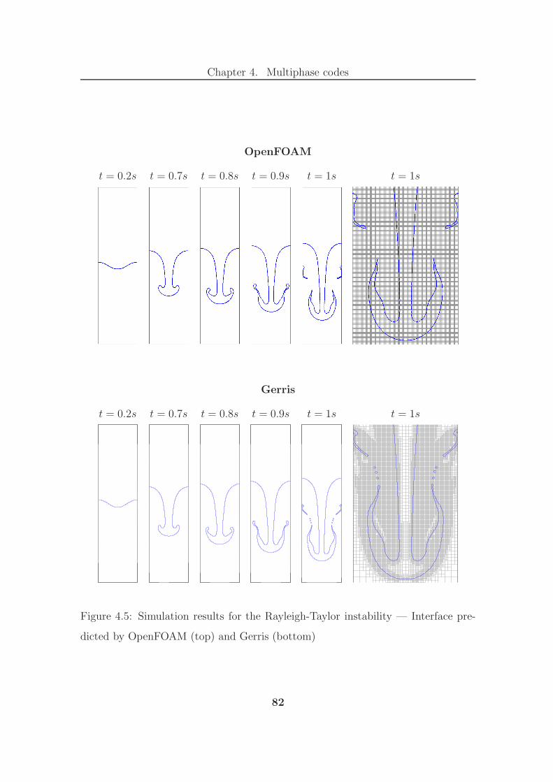
Chapter 4. Multiphase codes
OpenFOAM
t = 0.2s t = 0.7s t = 0.8s t = 0.9s t = 1s t = 1s
Gerris
t = 0.2s t = 0.7s t = 0.8s t = 0.9s t = 1s t = 1s
Figure 4.5: Simulation results for the Rayleigh-Taylor instability — Interface pre-
dicted by OpenFOAM (top) and Gerris (bottom)
82

Chapter 4. Multiphase codes
Original mesh — 128 × 512 Refined mesh — 256 × 1024
Figure 4.6: Performance of OpenFOAM on the simulation of the Rayleigh-Taylor
instability — Detail of the interface in the region of the neck at t = 1s for meshes:
128 × 512 (tcalc = 6126s) and 256 × 1024 (tcalc = 35688s)
83

Chapter 4. Multiphase codes
Constant mesh Adapted mesh Volume fractions Vorticity
Figure 4.7: Performance of Gerris on the simulation of the Rayleigh-Taylor instabil-
ity without surface tension — Results at t = 1s for constant mesh (Ncells = 65536 ;
tcalc = 1338s) and adapted mesh with lmax = 7 (Ncells = 24274 ; tcalc = 193s)
84
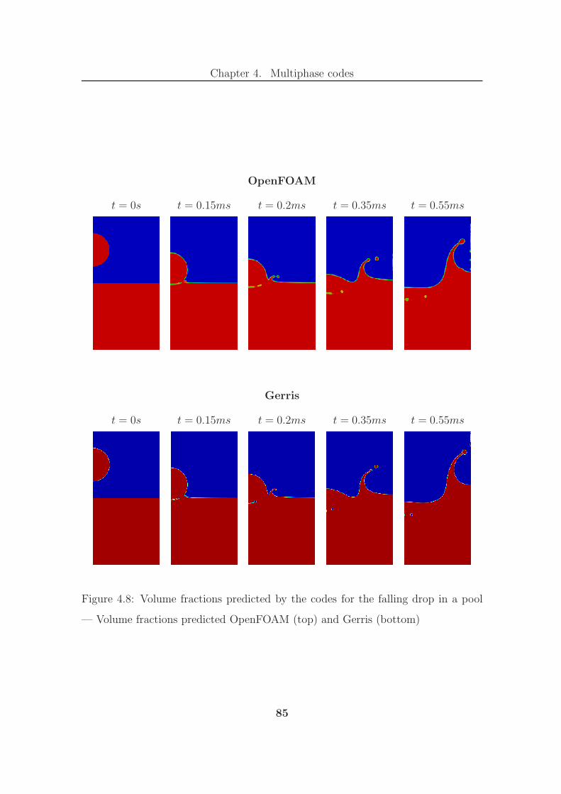
Chapter 4. Multiphase codes
OpenFOAM
t = 0s t = 0.15ms t = 0.2ms t = 0.35ms t = 0.55ms
Gerris
t = 0s t = 0.15ms t = 0.2ms t = 0.35ms t = 0.55ms
Figure 4.8: Volume fractions predicted by the codes for the falling drop in a pool
— Volume fractions predicted OpenFOAM (top) and Gerris (bottom)
85

Chapter 4. Multiphase codes
OpenFOAM OpenFOAM Gerris
1282 2562 1282
t = 1s
t = 2.25s
t = 4.5s
Figure 4.9: Volume fractions predicted by the codes for the phase inversion — Time
t = 1s, 2.25s, 4.5s
86
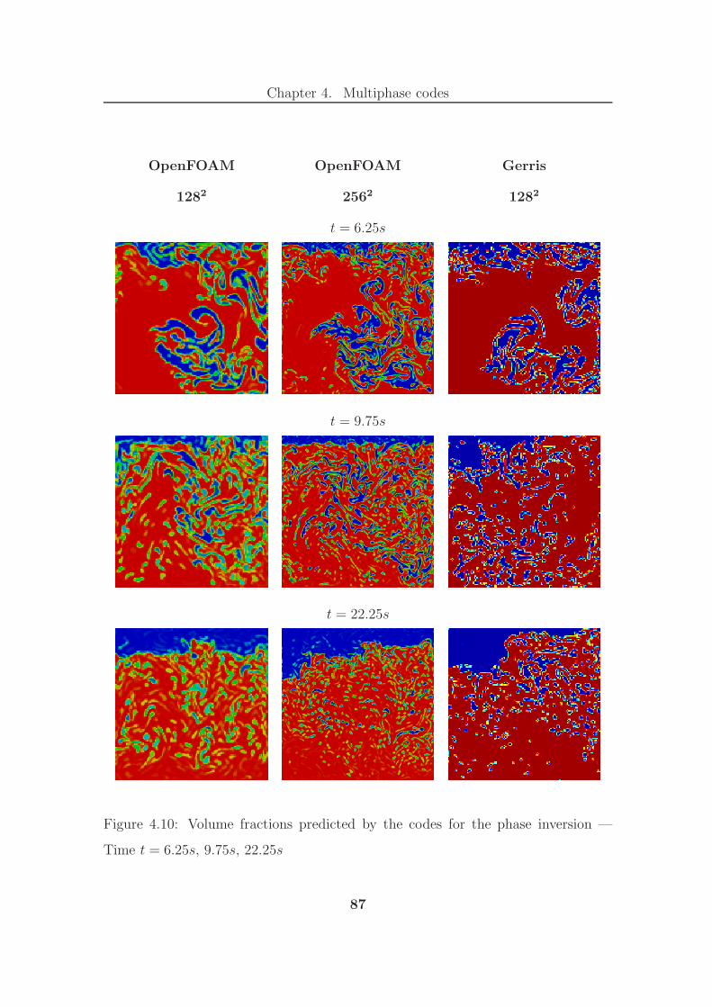
Chapter 4. Multiphase codes
OpenFOAM OpenFOAM Gerris
1282 2562 1282
t = 6.25s
t = 9.75s
t = 22.25s
Figure 4.10: Volume fractions predicted by the codes for the phase inversion —
Time t = 6.25s, 9.75s, 22.25s
87

Chapter 4. Multiphase codes
OpenFOAM OpenFOAM Gerris
1282 2562 1282
t = 34.75s
t = 42.25s
t = 100s
Figure 4.11: Volume fractions predicted by the codes for the phase inversion —
Time t = 34.75s, 42.25s, 100s
88

Chapter 4. Multiphase codes
4.3 Simulation of atomisation
Two types of simulation have been considered in order to take advantage of the best
features of both codes: the simulation of atomisation with sub-grid scale modelling,
using OpenFOAM (lesInterFoam, see [44] for details on SGS), and without, using
Gerris. The settings of all spray calculations are presented in tables 4.9, 4.10 and
4.11, and the corresponding non-dimensional numbers are given in Table 4.12.
The simulation of liquid breakup with SGS models involved reproducing the
results of Villiers et al. on the atomisation of Diesel jet [44] and extending this
approach (similar physical properties and domain dimensions) to the breakup of an
axisymmetric sheet. The latter calculation was done on a very coarse mesh as a
mean to illustrate the capability of OpenFOAM.
The simulations of flat sheet breakup without SGS models have been run using
Gerris with similar domain dimensions, fluid densities and surface tensions. How-
ever, in order to illustrate the effect of We on the spray, the viscosity has been
reduced for both fluids. Indeed, the turbulence in the flow field has a strong effect
on the primary breakup [54, 146] and to obtain a spray in a smaller computational
domain, we have artificially increase the Re in both phases. Also, as demonstrated in
experimental studies [135, 136, 145, 146, 195], thinning the vorticity layer increases
the growth rate of the interfacial instabilities and therefore reduces the breakup
length. The effect of the Weber number on the breakup (see Section 2.4) has been
illustrated on three simulations of increasing We. For the highest We, the build-up
of instabilities and the onset of the breakup are presented.
Due to the significant influence of turbulence build-up in the injection pipe [54,
146], the flow in the injection channel has been modelled for a distance of three to
five injection hole characteristic lengths depending on the configuration of the spray
calculation.
89

Chapter 4. Multiphase codes
Table 4.9: Physical properties for the spray calculations with SGS models
Fuel Gas Ratio fuel/gas
Density, ρ (kgm−3) 840 20 42
Viscosity, µ (kgm−1s−1) 5 × 10⁻³ 1.7 × 10⁻⁵ 294
Surface tension, σ (Nm−1) 2.61 × 10⁻²
Table 4.10: Physical properties for the spray calculations without SGS models
Fuel Gas Ratio fuel/gas
Density, ρ (kgm−3) 840 20 42
Viscosity, µ (kgm−1s−1) 5.952 × 10⁻⁶ 8.5 × 10⁻⁷ 7
Surface tension, σ (Nm−1) 2.61 × 10⁻²
90
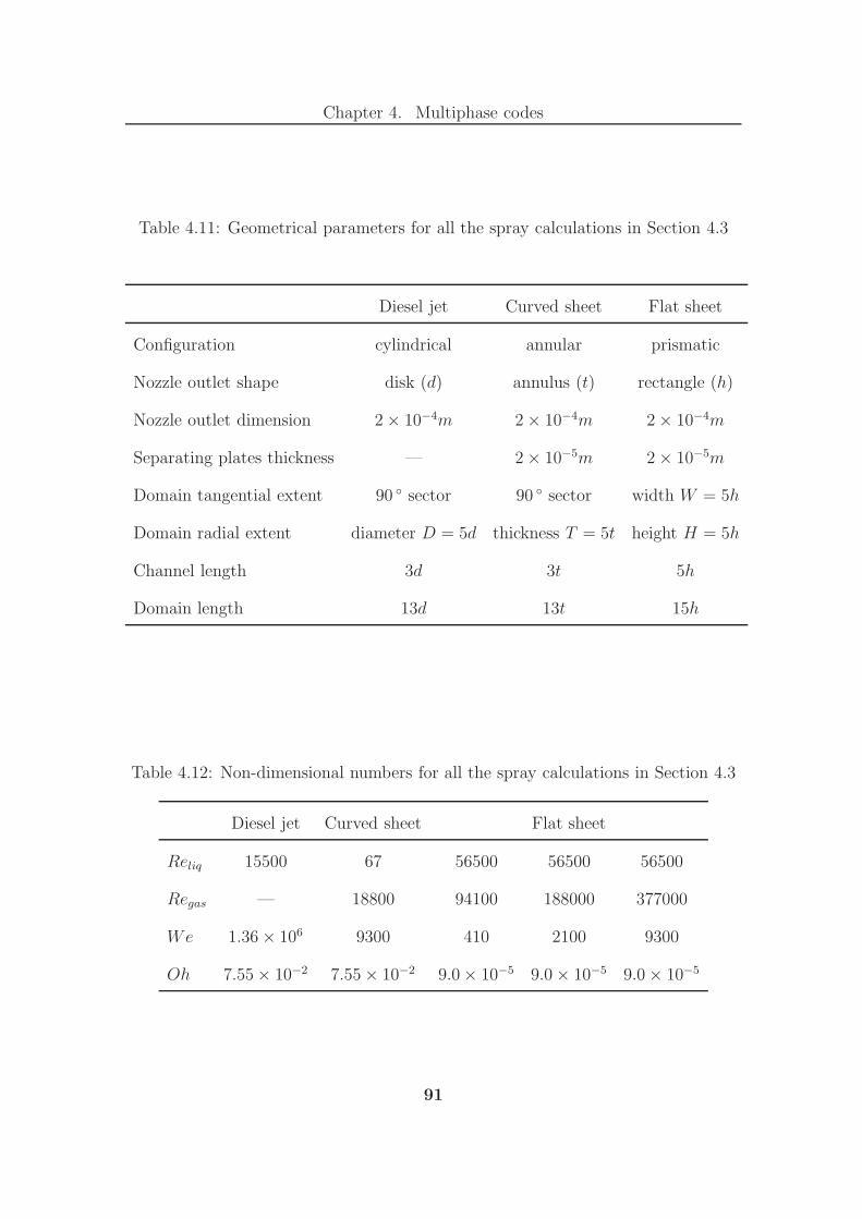
Chapter 4. Multiphase codes
Table 4.11: Geometrical parameters for all the spray calculations in Section 4.3
Diesel jet Curved sheet Flat sheet
Configuration cylindrical annular prismatic
Nozzle outlet shape disk (d) annulus (t) rectangle (h)
Nozzle outlet dimension 2 × 10⁻⁴m 2 × 10⁻⁴m 2 × 10⁻⁴m
Separating plates thickness — 2 × 10⁻⁵m 2 × 10⁻⁵m
Domain tangential extent 90 sector 90 sector width W = 5h
Domain radial extent diameter D = 5d thickness T = 5t height H = 5h
Channel length 3d 3t 5h
Domain length 13d 13t 15h
Table 4.12: Non-dimensional numbers for all the spray calculations in Section 4.3
Diesel jet Curved sheet Flat sheet
Reliq 15500 67 56500 56500 56500
Regas — 18800 94100 188000 377000
We 1.36 × 10⁶ 9300 410 2100 9300
Oh 7.55 × 10⁻² 7.55 × 10⁻² 9.0 × 10⁻⁵ 9.0 × 10⁻⁵ 9.0 × 10⁻⁵
91

Chapter 4. Multiphase codes
4.3.1 Simulations of liquid breakup with SGS model
The two geometries modelled with SGS models involve an axisymmetric configu-
ration (jet and annular sheet breakup). In order to keep the computational cost
reasonable, only a 90 sector has been modelled. No turbulence boundary condi-
tions have been set at the injection of the phases: it has been assumed that the
appropriate level of turbulence would be developed in the channels modelled. This
assumption would require sensitivity studies on the length of the pipe modelled and
the results should be compared with the outcome of the method of Klein et al. [112]
to generate velocity data artificially.
Diesel jet breakup Like all the simulation settings of this case, the mesh in
the radial direction is identical to the one shown in [44]. It can be found in one of
the tutorials of the lesInterFoam solver for a 2D geometry. The total number of cells
of this 90 sector (see Figure 4.12) is halfway between the coarse and fine meshes
in [44]. The overall refinement strategy for this mesh is geared to accommodate the
formation of small liquid structures at the interface. In particular, the highest level
of refinement is at the radius of the injection hole, in the vicinity of the nozzle outlet
to represent at best the instabilities triggering the onset of the breakup.
The simulation results have been commented and analysed in detail in [44] and
their validity is considered in Section 5.1.1. Only the first stages of the injection,
corresponding to the onset of the breakup, are presented in Figure 4.13 below.
The build-up of longitudinal waves along the interface is apparent in the injection
channel (t = 1 × 10⁻⁶s) and, once the jet has passed the nozzle outlet, in the vicinity
of the nozzle. However, the expected transverse instabilities, due to a Rayleigh-
Taylor type of instability [146], do not appear clearly until t = 3.508 × 10⁻⁶s when
thin ligaments start to form. This delay in the growth of these instabilities could
be due to incorrect levels of turbulence in the liquid or a lack of resolution in the
azimuthal direction.
92

Chapter 4. Multiphase codes
In addition, at t = 1 × 10⁻⁶s, some “dimples” are present along the interface at
the tip of the liquid jet. However, these features seem to follow the mesh too closely
and are certainly a numerical artefact due to the lack of resolution in the channel.
Further simulation on a finer mesh should address this question.
As explained in [44], the modelling of a sector when simulating jet breakup pre-
vents the jet to flap and consequently extends significantly the jet core length. In
particular, the large droplet at the tip of the jet (t = 3 × 10⁻⁶s) would have broken
off earlier in a full 3D simulation.
The expected gradual rise in vorticity magnitude and its spread is apparent on
the simulation results. This highlights the strong interaction between the turbulence
and the liquid structures and emphasised the need to develop sub-grid scale models
to better capture this phenomenon.
Axisymmetric sheet breakup This case is simply the extension of the Diesel
jet problem to an axisymmetric sheet breakup. The extent of the computational
domain is based on the same approach and the mesh has been designed with the
same philosophy (see Figure 4.14). In order to account for the effect of the separator
plates on the onset of the breakup (see [65]), the geometry modelled comprises
separator plates of finite thickness around which the mesh is particularly refined.
This case has been run in order to demonstrate OpenFOAM’s capability to simulate
sheet breakup. The mesh produced being very coarse, the analysis of the calculation
should be understood as provisional until further mesh convergence studies confirm
these results. No quantitative results should be expected from this simulation.
The same physical properties have been taken for the phases in presence but their
condition of injection have been modified to come closer to aero-engine conditions.
In particular, the gas stream is co-flowing (‖ugas‖ = 40ms−1) on either side of the
liquid sheet such that the atomisation is assisted. Also, the velocity of the fuel
injection has been reduced from ‖uliq‖ = 460ms−1 to ‖uliq‖ = 2ms−1. The resulting
non-dimensional number (We and Reliq) are significantly lower than for the Diesel
93

Chapter 4. Multiphase codes
jet case. The use of the exact same properties between the two cases allows direct
comparison of the performance of the injection systems. Besides, the properties of
the two phases in the Diesel jet injection and the aero-engine application, although
different, are of the same order of magnitude.
The earliest stages of the sheet atomisation are presented in Figure 4.15, from the
growth of interfacial waves, in the injection channel, to the onset of the breakup.
Longitudinal instabilities are clearly apparent on the simulation results from t =
4.5× 10⁻⁴s, on top of which transverse instabilities appear around t = 5.5× 10⁻⁴s.
Besides, the pattern of the vorticity contours originally (t = 1.54 × 10⁻⁴s) re-
sembles Von Karman streets as the gas is injected on either sides of the liquid
injection “crown”. The vorticity contours then evolve to a less structured pattern
(t = 3 × 10⁻⁴s) and the turbulent structures seem to interact with (potentially ini-
tiate) the flapping of the liquid sheet.
Two different breakup mechanisms have been identified in this calculation: one
resulting from the effect of the longitudinal wave (mechanism A, see Figure 4.16) and
the other one due the combined effect of both longitudinal and azimuthal instabilities
(mechanism B, see Figure 4.17).
The first mechanism involves the breakup of large liquid structures at the peak of
a longitudinal wave which then further fragments into streamwise ligaments, them-
selves breaking up into droplets under Plateau-Rayleigh instability.
The second mechanism leads to the formation of droplets through the combined
effect of instabilities in both longitudinal and transverse directions. The orthogonal
undulations stretch, and eventually tear, the liquid sheet at their peaks, leaving
liquid blobs at their nodes. This process is illustrated Figure 4.17, where the trans-
verse instability first tears the flapping liquid sheet in the longitudinal direction.
Then, a longitudinal wave, superimposed on the flapping mode, breaks up the large
longitudinal structures into droplets.
94

Chapter 4. Multiphase codes
Isometric view of the domain — 6.83 × 10⁵ cells
Detail of the nozzle outlet region
Figure 4.12: Simulation of Diesel jet breakup with OpenFOAM — Mesh of the
domain
95

Chapter 4. Multiphase codes
t = 1 × 10⁻⁶s t = 2 × 10⁻⁶s
t = 3 × 10⁻⁶s t = 3.508 × 10⁻⁶s
Figure 4.13: Simulation of Diesel jet breakup with OpenFOAM — Interface location,
volume fractions and vorticity contours for the onset of the breakup
96

Chapter 4. Multiphase codes
Isometric view of the domain — 1.86 × 10⁵ cells
Detail of the nozzle outlet region
Figure 4.14: Simulation of axisymmetric sheet breakup with OpenFOAM — Mesh
of the domain
97
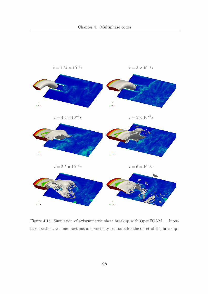
Chapter 4. Multiphase codes
t = 1.54 × 10⁻⁴s t = 3 × 10⁻⁴s
t = 4.5 × 10⁻⁴s t = 5 × 10⁻⁴s
t = 5.5 × 10⁻⁴s t = 6 × 10⁻⁴s
Figure 4.15: Simulation of axisymmetric sheet breakup with OpenFOAM — Inter-
face location, volume fractions and vorticity contours for the onset of the breakup
98

Chapter 4. Multiphase codes
t = 8 × 10⁻⁴s t = 9 × 10⁻⁴s
t = 9.5 × 10⁻⁴s t = 9.7 × 10⁻⁴s
t = 9.8 × 10⁻⁴s t = 9.9 × 10⁻⁴s
Figure 4.16: Simulation of axisymmetric sheet breakup with OpenFOAM — Inter-
face location, volume fractions and vorticity contours for the breakup mechanism
A
99

Chapter 4. Multiphase codes
t = 1 × 10⁻³s t = 1.01 × 10⁻³s
t = 1.02 × 10⁻³s t = 1.03 × 10⁻³s
t = 1.04 × 10⁻³s t = 1.05 × 10⁻³s
Figure 4.17: Simulation of axisymmetric sheet breakup with OpenFOAM — Inter-
face location, volume fractions and vorticity contours for the breakup mechanism
B
100

Chapter 4. Multiphase codes
4.3.2 Simulations of sheet breakup without SGS model
Three calculations of flat sheet breakup are presented in this section, corresponding
to three different gas velocities and therefore three different Weber numbers. All of
these simulations have been run on the same geometry and with the same initial mesh
(see Figure 4.18, top part). The geometry modelled is derived from the simulation
of the axisymmetric sheet breakup and includes separator plates of finite thickness
as recommended in [65].
The mesh is statically refined in the region where the liquid phase is expected in
order to capture finer liquid structures. The resulting grid is then made up of cells
of two different sizes: ∆x = 7.8µm in central part of the domain, and ∆x = 15.6µm
elsewhere. During the calculation, it can happen that a small liquid structure,
originally captured in the refined part of the grid, reaches the coarse part of the
grid. Conveniently, when using statically refined mesh in Gerris, in such instance
the code will automatically refine the mesh around the liquid structure in order to
maintain its initial level of resolution (see Figure 4.18, bottom part). In the case of
the simulation of atomisation at high We, this generally results in the rise of the
cell count as the calculation time goes by.
Although very powerful for the calculation of multiphase flows, Gerris does not
include sub-grid scale models. Therefore the validity of any simulation with Gerris
(as it is currently), relies upon sufficient grid refinement to capture all the scales
of the multiphase flow (turbulence and liquid structures). Table 4.13 provides the
smallest scales of the multiphase flow: the Kolmogorov scale for both the liquid and
the gas phase, and the droplet diameter obtained at We = 10, when the surface
tension effects become important.
It is clear from this table that even at the lowest Weber number, none of the
Kolmogorov scales are captured by the calculation. This is also true for the smallest
liquid structures requiring at least two to five grid cells for a reasonable resolution.
In particular, for the simulation at the lowest Weber number (We = 410), the finest
101
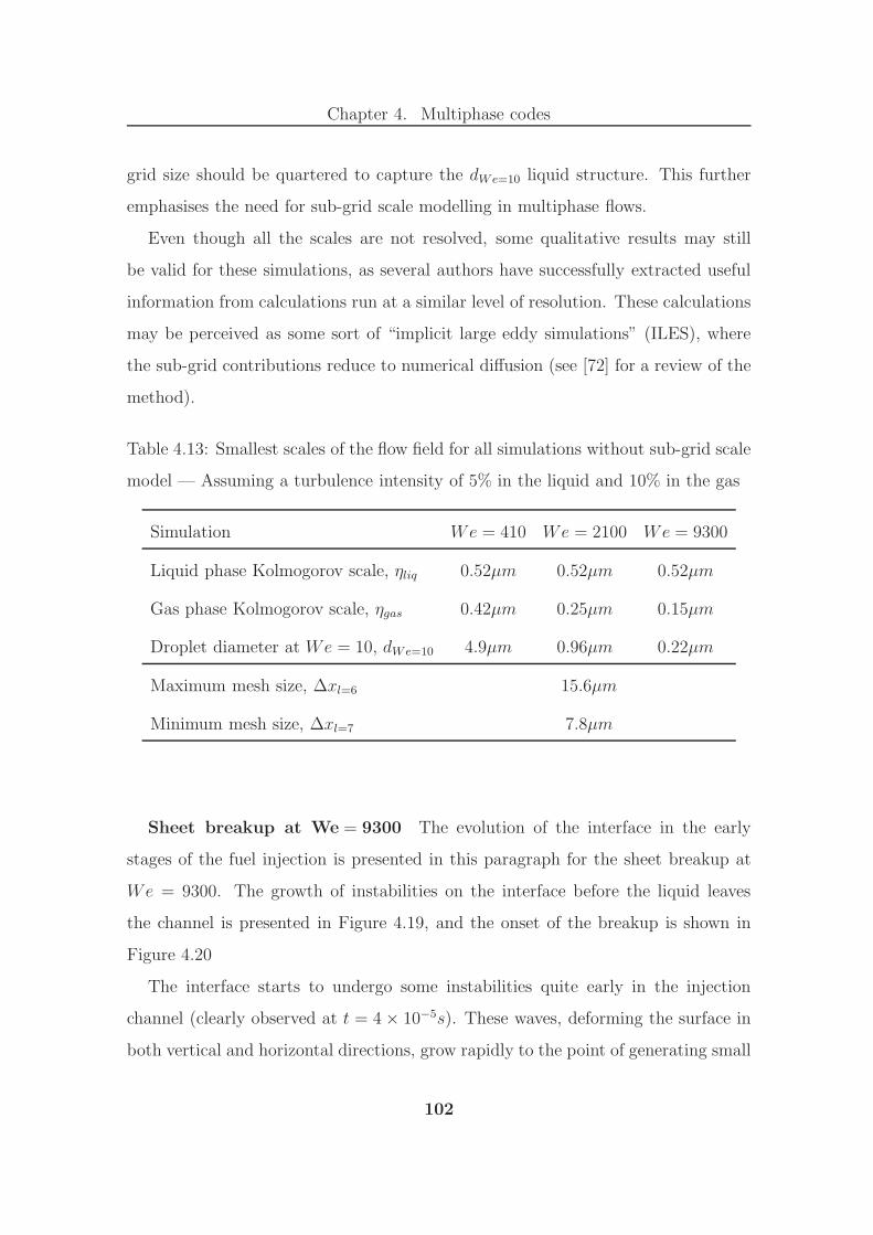
Chapter 4. Multiphase codes
grid size should be quartered to capture the dWe=10 liquid structure. This further
emphasises the need for sub-grid scale modelling in multiphase flows.
Even though all the scales are not resolved, some qualitative results may still
be valid for these simulations, as several authors have successfully extracted useful
information from calculations run at a similar level of resolution. These calculations
may be perceived as some sort of “implicit large eddy simulations” (ILES), where
the sub-grid contributions reduce to numerical diffusion (see [72] for a review of the
method).
Table 4.13: Smallest scales of the flow field for all simulations without sub-grid scale
model — Assuming a turbulence intensity of 5% in the liquid and 10% in the gas
Simulation We = 410 We = 2100 We = 9300
Liquid phase Kolmogorov scale, ηliq 0.52µm 0.52µm 0.52µm
Gas phase Kolmogorov scale, ηgas 0.42µm 0.25µm 0.15µm
Droplet diameter at We = 10, dWe=10 4.9µm 0.96µm 0.22µm
Maximum mesh size, ∆xl=6 15.6µm
Minimum mesh size, ∆xl=7 7.8µm
Sheet breakup at We = 9300 The evolution of the interface in the early
stages of the fuel injection is presented in this paragraph for the sheet breakup at
We = 9300. The growth of instabilities on the interface before the liquid leaves
the channel is presented in Figure 4.19, and the onset of the breakup is shown in
Figure 4.20
The interface starts to undergo some instabilities quite early in the injection
channel (clearly observed at t = 4 × 10⁻⁵s). These waves, deforming the surface in
both vertical and horizontal directions, grow rapidly to the point of generating small
102

Chapter 4. Multiphase codes
pockets of gas near the separator plates, on either side on the horizontal symmetry
plane (t = 4 × 10⁻⁵s).
At t = 1 × 10⁻⁴s the instabilities have deformed the interface so strongly that
some wave peaks announce the birth of ligaments, especially in the vicinity of the
small pockets of gas where the surface is the most distorted. At this time step, the
interface is already strongly asymmetric.
From t = 1 × 10⁻⁴s onwards, droplets start to form: this is the onset of the
breakup. The undulations start to produce distinctive “cells” at the interface with
sharper boundaries. The liquid phase covers parts of the separator plates, and from
the edges of these plates, at the location of the undulation peaks, thin ligaments are
growing and shedding droplets of similar diameter.
All through these early stages of the breakup, the vorticity contours present
patterns resembling Von Karman streets. These patterns of vorticity contours get
more and more complex as the calculation time goes by, but maintain roughly the
same large scale structures.
Effect of the We on sheet breakup The effect of the Weber number on
the sheet breakup has been illustrated with three simulations run at increasing
gas velocities, and therefore increasing We. The different breakup configurations
obtained are shown in Figure 4.21, Figure 4.22 and Figure 4.23.
At low Weber number, We = 410, the liquid bulk extends downstream of the
injection point and relatively thick ligaments are produced, leading to the breakup
into large droplets. When the Weber number is increased to 2100, the interface
adopts a totally different topology characterised by a shorter liquid bulk. At such
conditions, the ligaments and droplets produced are much smaller and spread further
outwards from the injection plane leading to a wider spray angle. When increasing
the Weber number to 9300, similar trends are observed with the shortening of the
liquid bulk and the decrease of the mean ligament thickness and droplet diameter.
It is worth mentioning that all three simulations of atomisation eventually lead
103

Chapter 4. Multiphase codes
to the formation of non-physical cylindrical liquid structures in the middle of the
computational domain. This further emphasise the fact that Gerris’ development is
still ongoing and that this code is aimed at academic research rather than component
design.
104
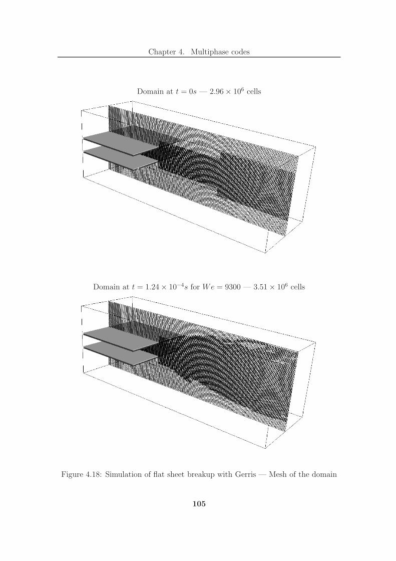
Chapter 4. Multiphase codes
Domain at t = 0s — 2.96 × 10⁶ cells
Domain at t = 1.24 × 10⁻⁴s for We = 9300 — 3.51 × 10⁶ cells
Figure 4.18: Simulation of flat sheet breakup with Gerris — Mesh of the domain
105
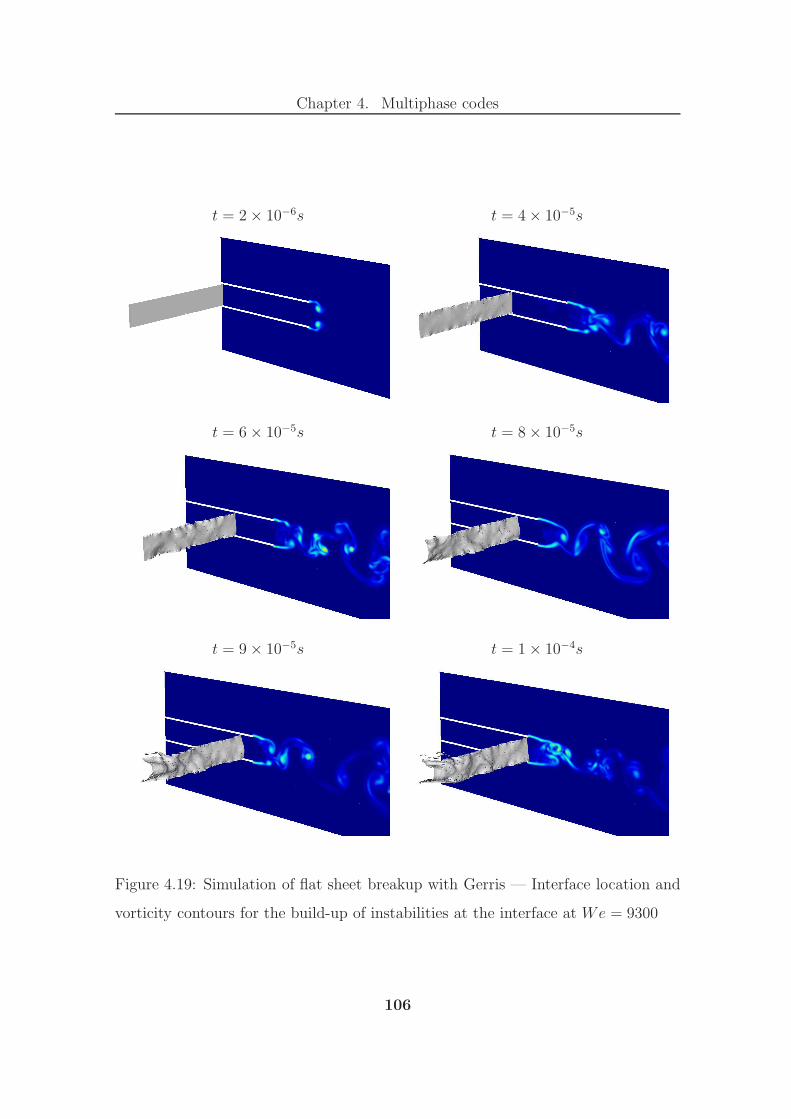
Chapter 4. Multiphase codes
t = 2 × 10⁻⁶s t = 4 × 10⁻⁵s
t = 6 × 10⁻⁵s t = 8 × 10⁻⁵s
t = 9 × 10⁻⁵s t = 1 × 10⁻⁴s
Figure 4.19: Simulation of flat sheet breakup with Gerris — Interface location and
vorticity contours for the build-up of instabilities at the interface at We = 9300
106
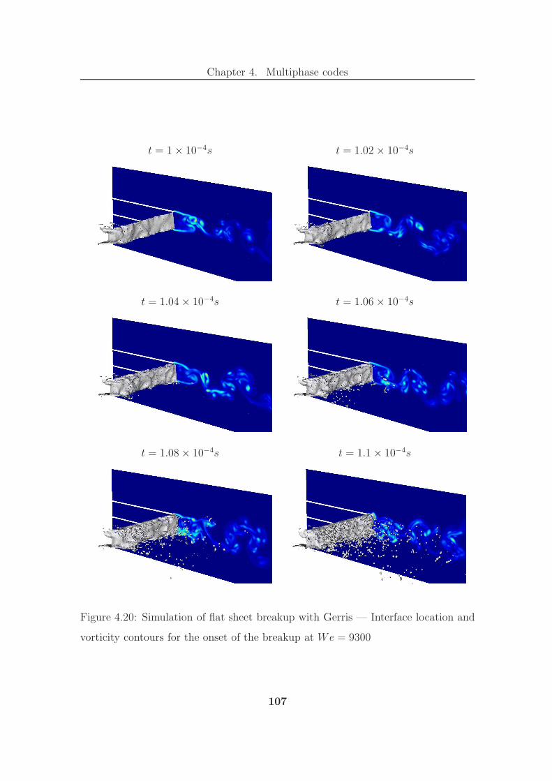
Chapter 4. Multiphase codes
t = 1 × 10⁻⁴s t = 1.02 × 10⁻⁴s
t = 1.04 × 10⁻⁴s t = 1.06 × 10⁻⁴s
t = 1.08 × 10⁻⁴s t = 1.1 × 10⁻⁴s
Figure 4.20: Simulation of flat sheet breakup with Gerris — Interface location and
vorticity contours for the onset of the breakup at We = 9300
107

Chapter 4. Multiphase codes
Figure 4.21: Simulation of flat sheet breakup with Gerris — Interface location,
velocity magnitude and vorticity contours at We = 410 (t = 1.78 × 10⁻⁴s)
108

Chapter 4. Multiphase codes
Figure 4.22: Simulation of flat sheet breakup with Gerris — Interface location,
velocity magnitude and vorticity contours at We = 2100 (t = 1.54 × 10⁻⁴s)
109

Chapter 4. Multiphase codes
Figure 4.23: Simulation of flat sheet breakup with Gerris — Interface location,
velocity magnitude and vorticity contours at We = 9300 (t = 1.24 × 10⁻⁴s)
110

Chapter 5
Atomisation modelling
The design of injectors relies heavily on testing as no numerical method has so
far been able to provide validated quantitative results on a real air-blast atomiser
geometry. However, in the past years this problem has attracted the interest of
many scientists who have developed a broad variety of approaches to come closer to
simulating the atomisation process and understand real injection systems.
The main successful attempts to model the atomisation process on simplified
configurations are presented in Section 5.1. Then, in Section 5.2, we review the
current approaches adopted by scientists to extend their modelling capability to the
simulation of real engine geometries. Finally, in Section 5.3, we detail our strategy
to simulate the fuel injection in a combustion chamber.
5.1 Demonstrated numerical capabilities
5.1.1 LES with VOF
The LES-VOF approach of Villiers et al. [44] has been applied to Diesel jet breakup
using OpenFOAM. Even though the droplet size distribution obtained showed a
strong grid dependency, the results of the simulations compared successfully with
spray angle and liquid core length measurements. In this study of the atomisation
111

Chapter 5. Atomisation modelling
with LES, the authors primarily assumed that the unresolved eddies, surface pertur-
bations and droplets did not affect the onset of the breakup. In addition, the method
neglects the sub-grid scale effects of the surface tension and the interface-turbulence
interaction.
Despite the poor VOF method employed (see Chapter 4), the calculations picked
up the non-linear growth of Kelvin-Helmholtz instabilities along the jet surface but
did not reproduce the mushroom shape (see Figure 5.1) typical of Diesel jets [150,
152]. The study also highlighted the sensitivity of the onset of the breakup to the
turbulence generated in the nozzle upstream of the injection point. In addition,
the comparison of a 90 sector simulation with full 3D calculations emphasised the
three-dimensionality of the primary breakup. Sector models lead to the artificial
limitation of the large scales of motion resulting in erroneous predictions of breakup
length and spray angle.
Figure 5.1: LES-VOF simulation of a Diesel spray atomisation (full 3D, ∆xmin =
10µm, pipe L/D > 40) [44] — Contour of volume fraction
In their study, Villiers et al. assessed the degree of atomisation with the mean
surface density, which increases with the level of interface distortion and with the
concentration of small droplets. The analysis of the atomisation (droplet sizes and
shapes) implied that breakup calculations reproduced the relative importance of
surface tension, aerodynamic forces and inertia according to the scale considered.
112

Chapter 5. Atomisation modelling
In particular, the dominant influence of surface tension at small scales was illustrated
by the spherical shape of small droplets whereas the predominance of aerodynamic
forces and inertia at large scales was suggested by the elongated shape of the large
liquid structures.
The effect of turbulence in the injection channel was also investigated qualitatively
by Bianchi et al. using an LES-VOF approach [19]. Further simulations of Bianchi
et al. [18] on a finer mesh (∆x = cst = 4µm) produced quantitative information
about the effect of the nozzle regime on the atomisation process (see Figure 5.2). In
particular, the authors noted that this phenomenon affected strongly the core length
and the atomised mass but had almost no impact on the droplet size distribution
because of the very high Weber number We, and Ohnesorge number Oh, of the
liquid jet.
(a) (b)
Figure 5.2: LES-VOF simulation of a Diesel spray atomisation (∆x = 4µm) —
Effect of nozzle regime on the liquid surface perturbations at the injection point
[18]: (a) Renozzle = 1625; (b) Renozzle = 8725
5.1.2 VOF with adaptive mesh refinement
Fuster et al. ran the VOF-AMR code Gerris [183] to simulate a hollow-cone atomiser
at realistic automotive injection conditions [65]. In this work, the vorticity and the
gradient of the tracer variable were used as criteria for the mesh refinement.
113

Chapter 5. Atomisation modelling
At first, Fuster et al. validated the code’s capability to capture the behaviour
of instabilities against the predictions of the viscous linear theory. In particular,
Gerris matched the theoretical predictions for the temporal growth of disturbances
within 5% for a broad range of conditions (parameters: density and viscosity ratios,
surface tension).
Then, solving all the scales of the turbulence in both phases, the authors studied
the onset of the instabilities, on a jet in co-flow, assuming that the unresolved
liquid structures do not affect the appearance of waves on the interface. The high
Re simulations, run in 2D (complex flow field, high resolution: ∆xmin = 0.8µm),
relied on a random vertical velocity (in the gas or the liquid phase) to trigger the
instabilities; therefore avoiding the need to introduce any geometrical parameters
in the analysis. In contrast, the low Re simulations, run in 3D, relied only on
the modelled separator plate and the difference in inlet velocities to destabilise the
interface.
The high Re calculations pointed out that the onset of the instabilities is strongly
related to the turbulence at the inlet of both phases and that the amplification of
the waves leads to the transition into the non-linear regime. These simulations also
highlighted the sensitivity of the modes to the evolution of the bulk flow downstream
(changes in velocity profiles, thickening of the boundary layer). Although good
agreement was obtained with the theory in the linear part of the jet, the three-
dimensionality of the flow — essentially downstream of the transition into the non-
linear regime — suggested that 2D calculations were unsuitable for regions of the
flow in the non-linear regime.
The low Re cases, run in 3D, captured the transverse instabilities that appear
further downstream of the injection point. These simulations confirmed the two-
dimensionality of the jet near the inlet and therefore tended to validate the 2D
approach at the beginning of the linear regime region (before the growth of transverse
instabilities). The addition of some injector geometry to the computational domain
demonstrated the influence of both the thickness of the separating plate and the
114

Chapter 5. Atomisation modelling
vortices produced in the injection channels. In particular, these vortices appeared
to affect significantly the primary breakup process and interacted strongly with the
droplets generated.
Finally, Fuster et al. conducted a parametric CFD study of swirl-atomisers, inves-
tigated the sensitivity of the solution under grid refinement and validated their calcu-
lations((ρliq/ρgas)CFD = 30/1
)against experimental results
((ρliq/ρgas)EXP = 700/5
).
The numerical results appeared to be very sensitive to mesh refinement (see Fig-
ure 5.3) for both the small structures of the flow (droplets) and the big features of
the spray (spray angle, breakup length). However, despite a significant difference in
density ratio, the high resolution simulation (∆xmin = 9µm) reproduced the general
features of the spray (cone angle, change of slope, breakup length) and the droplet
size distribution. Because of the breadth of scales involved in the atomisation pro-
cess, the simulation of the whole system is required to understand the operation of
real injectors. This has been made possible — for a simple fuel injector — thanks
to the use of adaptive meshing techniques that handle these issues efficiently.
(a) (b) (c)
Figure 5.3: VOF simulation of a swirl outward-opening jet (full 3D) [65] — Contour
of volume fraction in a median for various mesh sizes: (a) ∆xmin = 56µm; (b)
∆xmin = 28µm; (c) ∆xmin = 9µm
115
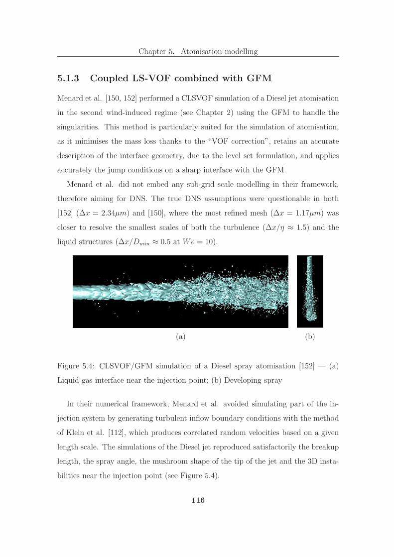
Chapter 5. Atomisation modelling
5.1.3 Coupled LS-VOF combined with GFM
Menard et al. [150, 152] performed a CLSVOF simulation of a Diesel jet atomisation
in the second wind-induced regime (see Chapter 2) using the GFM to handle the
singularities. This method is particularly suited for the simulation of atomisation,
as it minimises the mass loss thanks to the “VOF correction”, retains an accurate
description of the interface geometry, due to the level set formulation, and applies
accurately the jump conditions on a sharp interface with the GFM.
Menard et al. did not embed any sub-grid scale modelling in their framework,
therefore aiming for DNS. The true DNS assumptions were questionable in both
[152] (∆x = 2.34µm) and [150], where the most refined mesh (∆x = 1.17µm) was
closer to resolve the smallest scales of both the turbulence (∆x/η ≈ 1.5) and the
liquid structures (∆x/Dmin ≈ 0.5 at We = 10).
(a) (b)
Figure 5.4: CLSVOF/GFM simulation of a Diesel spray atomisation [152] — (a)
Liquid-gas interface near the injection point; (b) Developing spray
In their numerical framework, Menard et al. avoided simulating part of the in-
jection system by generating turbulent inflow boundary conditions with the method
of Klein et al. [112], which produces correlated random velocities based on a given
length scale. The simulations of the Diesel jet reproduced satisfactorily the breakup
length, the spray angle, the mushroom shape of the tip of the jet and the 3D insta-
bilities near the injection point (see Figure 5.4).
116

Chapter 5. Atomisation modelling
Nevertheless, in their analysis of the evolution of the droplet distribution under
grid refinement, the authors noted that the insufficient level of resolution affected
their calculations. In particular, they concluded that the coarseness of the grid
resulted in the predominant occurrence of a “numerical” breakup process for both
droplets and thin ligaments. However, on instances of physical breakup, these cal-
culations matched the prediction of droplet sizes as a function of ligament thickness
given in [146].
5.1.4 RLSG combined with Lagrangian tracking
Kim et al. have combined the RLSG-balance force method of Herrmann [86] with
the Lagrangian tracking of small droplets to produce near DNS of a liquid jet in
co-flow [111]. The settings of the simulation match the experimental conditions
of [146]. Kim et al. introduced a novel procedure to take small spherical liquid
structures (i.e. no ligaments) out of the level set formulation in order to transfer
them into a “Lagrangian stochastic spray” model.
The transfer of droplets into a Lagrangian spray model saves computational time
while retaining an accurate description of the liquid phase. Indeed, the atomisation
process produces a large amount of droplets and describing all the liquid struc-
tures with a level set formulation becomes very expensive in the early stages of the
development of the jet. In addition, Lagrangian spray models have demonstrated
satisfactory performance in the representation of the secondary breakup. However,
in [111], the transfer of droplets is only based on the size and the shape of the par-
ticle and does not account for the frequent occurrence of droplets re-entering the
bulk of the liquid [1].
The calculations showed qualitative agreement with the experimental results of
[146]. In particular, it reproduced the series of instabilities (longitudinal Kelvin-
Helmoltz followed by azimuthal Rayleigh-Taylor) leading to the formation of liga-
ments. The ligament’s stretching, pinch off and breakup under Plateau-Rayleigh
117

Chapter 5. Atomisation modelling
instability were also satisfactorily reproduced (see Figure 5.5). However, as in
[44, 150, 152], the droplet size distribution appeared grid dependent and the peak
of the droplet size distribution was also obtained for a droplet diameter of twice the
minimum grid size. Kim et al. still claimed some level of grid-convergence of the
droplet size distribution for droplets larger than two G-grid cells (finest grid size in
the RLSG framework).
(a) (b)
Figure 5.5: Round liquid jet sheared by co-flowing air (Regas = 3770 ; Reliq = 295)
— (a) Experiments [146]; (b) RLSG/Lagrangian tracking simulation [111]
5.1.5 Conservative LS with GFM
Desjardins et al. modelled Diesel jet atomisation with an improved CLS method
combined with the GFM to treat the singularities [47]. This method maintains
satisfactory mass conservation — required for the stability of the calculation and
the accuracy of the results — at a much lower computational cost than the CLSVOF
method of Menard et al. [150, 152]. Desjardins et al. did not include any sub-grid
scale models, therefore aiming for DNS with a constant grid size of ∆x = 3.9µm.
However, Desjardins et al. did not extract any quantitative information from their
simulation, conscious that true DNS would not be reached with such resolution.
118

Chapter 5. Atomisation modelling
The simulation domain and conditions were similar to [152] but did not include
any turbulent inflow conditions nor any modelling of the injection channel. Although
this questions the realism of this simulation, as most authors [18, 19, 44, 146] ac-
knowledged the importance of this factor, it facilitated the study of the induction
of turbulence in the gas phase by the resulting jet. In particular, Desjardins et al.
highlighted annular vortical structures generated by the jet in the gas and reported
their strong interactions with liquid structures.
(a)
(b)(c)
Figure 5.6: CLS/GFM of Diesel spray atomisation [47] — (a) “Mushroom shape”
of the jet tip shedding droplets; (b) Ligament formation and breakup; (c) Detail of
the liquid structures
5.2 Towards an industry-friendly approach
5.2.1 Development of sub-grid scale models
Most importantly, the main authors have realised the need to develop models for the
sub-grid contribution of the interface (in particular for LES of atomisation). As the
thickness of the interface is of the order of a few tenths of nanometres, the resolution
requirements for representing the smallest liquid structure in the case of a topology
change (“zero-sized connecting ligament at the very instance of the breakup” [71])
119

Chapter 5. Atomisation modelling
would be unmanageable in the simulation of turbulent primary breakup; let alone
the violation of the continuum assumption of the Navier-Stokes equations. There-
fore, the generation of sub-grid scale models (droplet pinch off, interface-turbulence
interaction, interfacial sub-grid contributions, ligament breakup, etc . . . ) is essential
to produce numerical simulation of atomisation that carries a physical significance.
For this purpose, various authors are developing specific numerical methods that
embed a physical description of the interface [84, 118]. In this context, Van der
Waals-Cahn-Hilliard frameworks, such as the phase field methods [101], also seem
promising.
5.2.2 Realistic boundary conditions
Many authors have observed — both numerically and experimentally — the impor-
tance of the boundary conditions (inflow and geometry) on the liquid jet atomisation
and have identified the need to reproduce them accurately. The accurate applica-
tion of both the velocity profiles (boundary layers in liquid and gas phases — [146])
and the inlet turbulence [18, 44, 54] are critical to predict the onset of the breakup
and the growth of perturbations at the interface. In particular, the inlet turbulent
conditions have been prescribed in two different ways: some authors have simulated
the flow in the injector channels [18, 44] whereas others have developed specific
procedures [112, 150, 152] to avoid the extra computational cost of an extended
domain.
As pointed out by Fuster et al. [65], the understanding of real injection systems
requires the resolution of large scale turbulent structures as these eddies interact
with themselves and with the liquid particles. As a result, these vortices, resulting
from the geometry of the whole system, strongly influence the overall structure of
the spray and the final droplet distribution. This is further confirmed by the high
level of accuracy obtained by [6, 7, 67, 200] in the LES of atomising sprays with
stochastic modelling of secondary breakup.
120

Chapter 5. Atomisation modelling
In order to embed such a large amount of geometry in the numerical calculation,
the use of adaptive mesh refinement is an efficient way to deal with the breadth of
scales involved in the atomisation process [86, 182]. It is also necessary to optimise,
the use of computational power. For this purpose, Peng et al. developed a “narrow-
band” approach, for level set methods, that localises the resolution of the equations
of the interface-capturing method [173]. With the same aim of reducing the compu-
tational cost, Kim et al. transferred the small droplets from the interface-capturing
technique to a Lagrangian spray model [111]. This technique can be further im-
proved by implementing a criterion that accounts for the droplets re-entering the
bulk of the liquid phase. More generally, the authors have concentrated their effort
on developing highly parallelisable methods usually based on VOF and/or LS in-
terface description. Also, some authors have focussed on the development of LES
formulations for atomisation modelling. Such frameworks can include much more
geometry than DNS, which is never truly achieved in high Re atomisation.
5.2.3 Accurate description of the interface
The internal geometry of aero-engine injectors is very complex and has a dominant
influence on the spray pattern. In order to account for the effect of these geometrical
details on the spray characteristics, the numerical frameworks have to embed a
method to capture the interface. As none of the available methods have satisfactorily
described the atomisation, the development of interface description methods is on-
going.
In the recent years, many authors have invested a lot of effort in the correction
of the flaws of the existing methods. More precisely, in the case of VOF interface-
capturing techniques, significant improvements have been made on the treatment of
surface tension [59, 183] and the reconstruction and the advection of the interface
(see [178] for a review). For level set methods, the mass conservation properties
have been enhanced either by coupling with VOF (CLSVOF — [25, 150, 152, 243])
121

Chapter 5. Atomisation modelling
or, more cheaply, by modifying the scalar advected (CLS — [47, 163]).
The hybridising of existing interface description methods has been very popu-
lar in the past ten years. In particular, the LS, VOF and marker methods have
been coupled — two by two — to combine the relative advantages of the different
techniques. Although these approaches have usually given accurate results, they
generally involve high computational cost [53, 133, 150, 152, 185]. In addition to
that drawback, the coupling with surface marker particles is in general very difficult
to extend to 3D and does not always represent physically the sub-grid scales of the
hydrodynamic field [217].
The difficulty of developing efficient new ways of describing the interface and
the complexity involved in the correction of the existing techniques have led many
scientists to consider transforming obsolete or “exotic” methods developed in other
fields of science. For instance, the smoothed particle hydrodynamics (SPH) of Gin-
gold and Monaghan [68], originally developed for astrophysics calculations, seems
to attract a lot of interest nowadays. Although these methods tackle the problem of
primary breakup with a fresh perspective, they do not generally describe multiphase
flow problems with the appropriate physics.
5.2.4 Numerical implementation of the physics
The challenge of handling the complex physics involved in the atomisation process
is directly related to the treatment of the interface. The numerical description of
material discontinuities and surface tension has been tackled with significant success
in the past years. In particular, Fedkiw et al. have produced the ghost fluid method
[55] — essentially directed towards LS formulations — that retains a sharp interface
while accurately applying the jump conditions. Furthermore, the popular contin-
uum surface force method has been significantly improved by Francois et al. who
produced a “balanced force algorithm” [59] to maintain the exact balance between
the surface tension forces and the pressure jump across the interface. These methods
122

Chapter 5. Atomisation modelling
have significantly reduced the occurrence of unphysical velocities (spurious currents)
near the interface and the focus is on the development of accurate calculations of
the interface curvature [86, 183, 198] to fully address this problem.
The addition of the compressibility effects in multiphase flows (e.g. [154] for VOF,
[157] for LS) has been considered by few authors. Tanguy and Menard [150, 246]
have noticed the potential need for a compressible formulation from code instabil-
ities arising in the simulation of pockets of gas trapped between liquid membranes
during the formation of ligaments. Considering the simplifications resulting from
the incompressible formulation and taking into account the large amount of work
invested in the development of dedicated numerical schemes, the generation of an
efficient compressible multiphase solver remains also a challenge.
5.2.5 Summary
The main authors have pursued the development of the following fields to improve
the simulation of atomisation:
• Generation of SGS models for LES of atomisation
• Development of hybrid interface description methods to maximise the advan-
tages of the different techniques
• Correction of VOF and LS flaws
• Adaptive mesh strategies
• Simulation of primary breakup with a compressible formulation
• Lagrangian tracking of small droplets
More practically, the understanding of primary breakup and more generally the
successful simulation of high Re atomisation is of particular relevance to the numer-
ical calculation of the reacting flow in combustion chambers. Therefore, in order
123

Chapter 5. Atomisation modelling
to focus the generation of methods on the industrial problem, there is a need to
assess the droplet size below which the liquid structures have negligible effects on
the reacting flow.
Furthermore, with the advent of high pressure propulsion systems, the injection
of fuel may occur at supercritical conditions. In such an environment, the surface
tension becomes negligible and the concept of interface is questionable [71]. Just like
the computation of primary breakup, the numerical simulation of “supercritical fuel
injection” is an open field of research with strong implications for both the industry
and the environment.
5.3 A modelling capability for fuel-injector design
Now that the state-of-the-art and the current trends in atomisation modelling have
been presented, this section provides the structure of the CFD capability developed
to simulate the atomisation process in aero-engine combustors.
The requirements of the industry are listed in Section 5.3.1 and the strategy
adopted to meet these objectives is detailed in Section 5.3.2. Then, the structure of
the resulting modelling tool is outlined in Section 5.3.3.
5.3.1 Industry requirements
To satisfy the industry’s need for a modelling capability simulating fuel-injection,
this project has focussed on the following criteria to develop a novel multiphase flow
solver:
• Handling of the complex geometries of modern aero-engines fuel injectors.
• Fast computations to provide results within engineering time scales.
• Accurate calculations to capture the physics of the atomisation.
• Mass conservation of the liquid fuel.
124
Chapter 5. Atomisation modelling
• Robust numerical formulation to ensure simulation convergence for all oper-
ating conditions.
• Production of data ready to be exploited by combustion codes.
• Parallelised solver to make the most of the available computational power.
5.3.2 Modelling strategy
In order to represent faithfully the geometry of the injection device in a timely man-
ner, the method developed is geared towards general unstructured grids. Besides,
as unstructured meshes are generally faster to generate, the use of such numerical
methods allows to significantly reduce the mesh generation task of the CFD design
study.
As CFD studies need to satisfy engineering time scales without compromising on
the quality of the calculation, our approach maximises the amount of pre-processing
operations. Once stored in text files, the mesh-dependent variables can be read
directly before any new calculation on a given mesh. It results that the amount of
run-time operations required is minimal and that high-order schemes run as fast as
low-order ones. Since a given geometry will be tested at many different conditions
with the same mesh, this pre-processing strategy makes the overall CFD study very
efficient.
In addition, the mass conservation of the fuel present in the flow field is critical
to accurate combustion predictions. As the solver developed can also be used as a
sub-model for combustor design, the two-phase flow modelling is based on an im-
proved conservative level set method that ensures mass conservation while remaining
cheaper than accurate coupled level set-VOF.
The modelling capability has been implemented with a WENO scheme developed
for unstructured meshes [186, 187]. In our numerical experiments, moving from the
high-order linear to the WENO formulation of the scheme has proven to increase
125

Chapter 5. Atomisation modelling
dramatically the stability of the method in the case of very large density ratios (see
Section 8.4). In particular, our modelling capability has demonstrated significantly
more robustness than the low-order method of OpenFOAM on the falling droplet
case of Sussman et al. [241].
The method outputs droplet fields and statistics that can be directly imported
into Lagrange tracking solvers for combustion modelling purposes. The dataset
produced by the multiphase modelling capability is also useful to analyse the per-
formance of a given injector design. Once identified in the flow-field, the droplets
are removed from the level set field and transferred into a droplet field. With this
approach the atomisation process is described accurately at a lower computational
cost.
Finally, a significant amount of effort as been placed in the parallel implemen-
tation of the method. It involved parallelising the unstructured numerical scheme,
the novel conservative level set method and the droplet transfer.
5.3.3 Outline of the solver
As mentioned in the previous sub-section, the code involves both pre-processing
and run-time operations. The pre-processing being only performed once on a given
mesh. The pre-processing operations involve producing mesh dependant variables
for:
• The high-order scheme developed for general unstructured meshes (see Chap-
ter 6). Most of the pre-processing computational time is devoted to that task.
• The high-order gradient involved in the interface normal calculation (see Sec-
tion 7.3).
• The transfer of droplets (see Section 8.2).
• The parallel run of the method (see Section 8.3).
126

Chapter 5. Atomisation modelling
For the run-time operations, the modelling capability developed presents the
following structure:
1. Update of the physical properties of the multiphase flow-field according to the
liquid volume fraction.
2. Transport of the liquid volume fraction represented by a conservative level set
field.
3. Calculation of the surface tension term.
4. Update of the turbulence properties if using a LES framework.
5. Pressure-velocity coupling as described in [208]. The discretised momentum
equation is first constructed and then a “correction loop” is performed. At
each iteration of that loop the pressure equation is solved and the momentum
is corrected based on the pressure change.
6. Transfer of droplets from the level set field to the “Drops” field and output of
the discrete phase characteristics.
In the generation of this numerical tool, the main focus has been placed on the
development of a novel high-order scheme for unstructured meshes (see Chapter 6)
and the production of a robust conservative level set method (see Chapter 7). These
essential building blocks of the new modelling capability produced have then been
implemented in parallel with an algorithm to output droplet fields and characteristics
(see Chapter 8).
127

Chapter 6
A high-order scheme for general
unstructured meshes
In this chapter, we detail the methodology developed, and implemented in parallel,
to construct high-order schemes — linear and WENO — on 3D mixed-element
unstructured meshes, consisting of general convex polyhedra. This numerical scheme
can formally reach arbitrarily high order of accuracy in space.
The construction of WENO schemes on 3D unstructured meshes is notoriously
difficult, as it involves a much higher level of complexity than 2D approaches. This
due to the multiplicity of geometrical considerations introduced by the extra dimen-
sion, especially on mixed-element meshes. Therefore, we have specifically developed
a number of algorithms to handle mixed-element meshes composed of convex poly-
hedra with convex polygonal faces.
The linear reconstruction procedure produced for 3D mixed-element unstruc-
tured grids is detailed in Section 6.3.1. Then, in Section 6.3.2, the main points of
the WENO reconstruction are presented. In Section 6.3.2, the computation of the
numerical flux is explained. The application of the technique to the solution of the
level set equation is considered in Section 6.4. Results are presented in Section 6.6
for a set of test cases in 2D and 3D.
128
Chapter 6. A high-order scheme for general unstructured meshes
6.1 WENO schemes for unstructured meshes
WENO schemes were originally developed for Cartesian grids [107, 131]. They
were an evolution of the essentially non-oscillatory (ENO) schemes introduced by
Harten et al. in 1987 [77, 78] to achieve high-order accuracy and non-oscillatory
properties near discontinuities such as shock waves in high-speed compressible flows.
As the interest in unstructured meshes grew, WENO schemes were constructed for
triangular [60, 95] and tetrahedral meshes [49, 50, 286]. However, the construction of
such schemes is much more complicated on unstructured meshes than on Cartesian
grids as no particular direction can be identified in the distribution of the elements.
The basic principles of the construction of WENO schemes for triangular meshes
were presented by Friedrich [60], based on the work of Abgrall [4]. Later, Dumbser
and Kaser extended these ideas to tetrahedral meshes [49] and defined an approach
to devise arbitrarily high-order schemes. Titarev et al. [254] improved this approach
for two-dimensional (2D) computational domains and produced high-order schemes
on mixed-element 2D meshes. We have extended the approach of Dumbser and
Kaser [49] and Titarev et al. [254] to 3D mixed-element unstructured grids for
linear hyperbolic equations [186]. In [187], we presented an extension of our scheme
[186] to general polyhedral cells and applied it to the solution of the level set equation
and the Burgers’ equation.
6.2 Overview of the numerical scheme
Looking ahead to the need to solve hyperbolic conservation laws to capture the
interface (see Chapter 7), the design of our high-order accurate numerical scheme
is based on two theorems: Godunov’s theorem [70] and the Lax-Wendroff theorem
[121]. The Lax-Wendroff theorem implies that if the hyperbolic conservation laws
are solved with conservative numerical schemes, the conserved variable — in our
case the smeared out liquid volume fraction (see Chapter 7) — should be conserved
129

Chapter 6. A high-order scheme for general unstructured meshes
exactly. As for Godunov’s theorem, it suggests that it is necessary to resort to a
non-linear numerical scheme (e.g. WENO) to reach a high order of accuracy without
generating oscillations.
The scope of the method is restricted to general hyperbolic systems of first-order
partial differential equations [49, 50]. Such systems may be expressed in 3D as:
∂
∂tU +
∂
∂xF (U) +
∂
∂yG (U) +
∂
∂zH (U) = 0 (6.1)
where U is the vector of conserved variables and F (U), G (U) and H (U) are the
vectors of the fluxes respectively in the x, y and z directions.
The computational domain is denoted by Ω and is discretised using conforming
elements Ei of volume |Ei| and boundary ∂Ei. Integrating (6.1) over the element
Ei leads to: ∫∫∫
Ei
∂
∂tU dEi +
∫∫∫
Ei
∇ · A dEi = 0 (6.2)
with the divergence of the second rank tensor A = (F,G,H) given by:
∇ · A =∂
∂xF (U) +
∂
∂yG (U) +
∂
∂zH (U)
Assuming that the control volume Ei is fixed and therefore independent of time t
and introducing Ui, the cell average of the conserved variables at time t, we can
re-write the first term on the left-hand-side (l.h.s.) of (6.2) as:
∫∫∫
Ei
∂
∂tU dEi =
d
dt
∫∫∫
Ei
U dEi = |Ei|d
dtUi (6.3)
Inserting (6.3) in (6.2), and applying the divergence theorem to the second term on
the l.h.s. of (6.2), leads to the finite volume formulation:
d
dtUi +
1
|Ei|
∫∫
∂Ei
A · n d(∂Ei) = 0 (6.4)
where n = (nx, ny, nz) is the outward unit vector normal to the surface ∂Ei and
A · n d(∂Ei) is the flux component normal to ∂Ei.
130

Chapter 6. A high-order scheme for general unstructured meshes
Splitting the integral over the contour of the element ∂Ei into Li integrals over the
faces Fl of Ei, and introducing the vector Anl= A · nl (nl being the outward unit
vector normal to Fl), we express the second term on the l.h.s. of (6.4) as:
∫∫
∂Ei
A · n d(∂Ei) =Li∑
l=1
∫∫
Fl
Anld(Fl) =
Li∑
l=1
Ail (6.5)
The inter-cell flux Ail associated with the face Fl of the element Ei is efficiently
calculated with a Gauss-Legendre quadrature of appropriate order. Inserting (6.5)
into (6.4) leads to:
d
dtUi +
1
|Ei|
Li∑
l=1
Ail = 0 (6.6)
In order to time-advance the cell-averages of the variables, the finite volume
scheme (6.6) requires the determination of the inter-cell fluxes. A reconstruction
operator is therefore necessary in each element Ei to provide the point-wise values of
the solution as needed by the flux evaluation. By using a polynomial reconstruction
operator, the finite volume method can reach arbitrarily high orders of accuracy
in space on any type of grid. If coupled with the ADER method of Toro et al.
[110, 221, 222, 252, 253, 256–258], this methodology would lead to a arbitrarily
high-order numerical scheme in both space and time. In this work, we coupled the
scheme with a Runge-Kutta time scheme which is theoretically limited in its order
of accuracy [3].
The difficulty is to design an efficient polynomial reconstruction that would allow
high-order accuracy while remaining cost-effective. A linear reconstruction operator
applied on a single stencil in general will produce spurious oscillations in the vicinity
of discontinuities. As multiphase flows systematically involve a severe discontinuity
(e.g. density jumps of several orders of magnitude) it is crucial to mitigate this
deficiency. For this purpose, we make use of weighted essentially non-oscillatory
(WENO) schemes [49, 95, 106, 107, 131, 186, 251, 285, 286]. The WENO recon-
struction is performed on unstructured meshes by applying a linear reconstruction
131
Chapter 6. A high-order scheme for general unstructured meshes
procedure to the various WENO stencils and combining the polynomials obtained
for each stencil, according to the solution-dependent weights.
A feature of the methodology presented here is the tetrahedral decomposition of
the mesh to handle the geometrical complexity of 3D mixed-element meshes. This
makes our technique quite general and appropriate for most industrial problems.
6.3 Numerical formulation
6.3.1 Methodology for the linear reconstruction
The linear reconstruction is presented in this section for a scalar variable, however its
extension to vector variables is straightforward. For each cell of the computational
domain, the linear reconstruction procedure produces a polynomial representing the
variable u (x, y, z, t) everywhere in the cell. The stencil S of cells Ej is used to
generate the interpolating polynomial on the targeted cell E0. For convenience the
first element of the stencil is the targeted cell. Hence:
S =
jmax⋃
j=0
Ej (6.7)
For each cell of the mesh, the polynomial p (x, y, z, t) is reconstructed from the
cell-averages of the variables in the cells of the associated stencil S. The reconstruc-
tion is performed with the constraint that the integral of the polynomial over the
targeted cell equals the cell-average value in this cell. This conservation condition
is expressed as:
u0 =1
|E0|
∫∫∫
E0
p (x, y, z) dx dy dz (6.8)
The polynomial reconstruction in physical coordinates x = (x, y, z) on a general
unstructured mesh requires the consideration of scaling effects. However, it is crucial
for the generality of the method to undertake the reconstruction in a reference space
ξ = (ξ, η, ζ) where scaling effects do not apply (see [49]). As well as elegantly
132
Chapter 6. A high-order scheme for general unstructured meshes
simplifying the polynomial reconstruction, working in a reference space prevents the
cumbersome introduction of inaccurate scaling factors.
It is necessary to relate the physical coordinates to the reference coordinates by
the mapping x = x (ξ, η, ζ). This operation requires the coordinates of four different
vertices of the targeted element Ei: one for the origin of the frame, and three others
— linked to the origin by an edge of Ei — to form the basis. For each cell in the
mesh, the inverse of this cell-dependent mapping: ξ = ξ (x, y, z) is applied to the
targeted cell and its stencil. This leads to a stencil in the reference space:
S ′ =
jmax⋃
j=0
E ′j (6.9)
Since the spatial average is not affected by the affine transformation ξ = ξ (x, y, z),
the conservation condition is also valid in the reference space. With p (ξ, η, ζ) defined
as the outcome of the polynomial reconstruction in the reference space, we have:
u0 =1
|E ′0|
∫∫∫
E′
0
p (ξ, η, ζ) dξ dη dζ (6.10)
To design a method for the determination of p (ξ, η, ζ), it is convenient to express
the polynomial in a basis of polynomial functions: φk (ξ, η, ζ)k=0...K . Introducing
the degrees of freedom ak, each associated to a given basis function, we write:
p (ξ, η, ζ) = u0 +
K∑
k=1
akφk (ξ, η, ζ) (6.11)
Therefore, the interpolating polynomial is completely defined by the set of (K + 1)
basis functions φk and their associated degrees of freedom ak. Also, the integer K
is related to the degree of the polynomial r by the expression:
K =(r + 1) (r + 2) (r + 3)
6− 1 (6.12)
The basis functions must be constructed so that the conservation condition (6.10)
is respected. This implies that the mean value of each basis function over E ′0 is null.
133

Chapter 6. A high-order scheme for general unstructured meshes
As in [254], we choose:
φk = ψk −1
|E ′0|
∫∫∫
E′
0
ψk dξ dη dζ (6.13)
where ψk = ξ, η, ζ, ξ2, ξ · η, . . . , ζr k = 1, . . . , K.
Knowing the basis functions, we can calculate the degrees of freedom ak by requir-
ing that the cell-averages of p (ξ, η, ζ) over each cell E ′j of the stencil S ′ is equal to
the corresponding cell-average of the variable: uj. This is expressed by the formula:
uj =1∣∣E ′j
∣∣
∫∫∫
E′
j
p (ξ, η, ζ) dξ dη dζ j = 1, · · · , jmax (6.14)
= u0 +
K∑
k=1
(1∣∣E ′j
∣∣
∫∫∫
E′
j
φk (ξ, η, ζ) dξ dη dζ
)ak j = 1, · · · , jmax (6.15)
= u0 +K∑
k=1
Ajkak j = 1, · · · , jmax (6.16)
where Ajk is the cell-average of the basis function φk over the cell E ′j of S ′.
Introducing bj = (uj − u0) in (6.16), the system of equations for the degrees of
freedom ak takes the matrix form:K∑
k=1
Ajkak = bj j = 1, · · · , jmax (6.17)
It can be seen from (6.15) and (6.17) that the reconstruction matrix A is solu-
tion independent. This means that the time-consuming operations required for the
determination of the ak can be pre-processed.
The solution of (6.17) provides the polynomial needed for the calculation of the
inter-cell fluxes (see Section 6.2). The determination of the fluxes depends on the
problem considered and on the Riemann solver chosen. The application of this
numerical method to the transport of the level set is detailed in Section 6.4.
Generation of a central stencil
In [186, 187], the stencil generation was performed by constructing — for each cell
of the domain — the most compact stencil S in the physical coordinate system
134
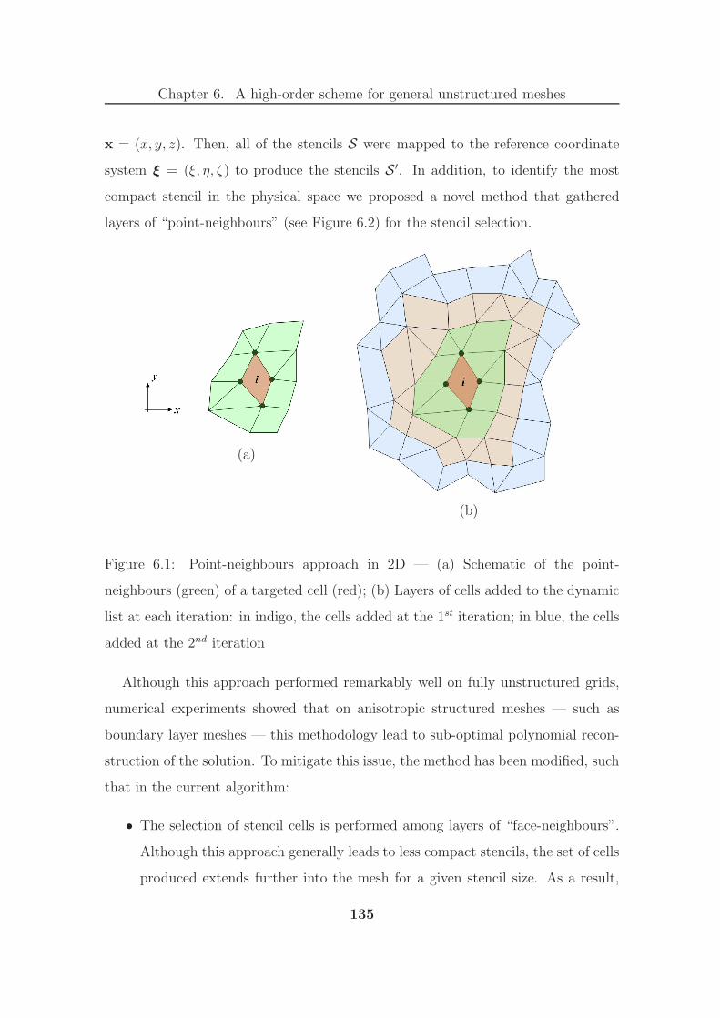
Chapter 6. A high-order scheme for general unstructured meshes
x = (x, y, z). Then, all of the stencils S were mapped to the reference coordinate
system ξ = (ξ, η, ζ) to produce the stencils S ′. In addition, to identify the most
compact stencil in the physical space we proposed a novel method that gathered
layers of “point-neighbours” (see Figure 6.2) for the stencil selection.
(a)
(b)
Figure 6.1: Point-neighbours approach in 2D — (a) Schematic of the point-
neighbours (green) of a targeted cell (red); (b) Layers of cells added to the dynamic
list at each iteration: in indigo, the cells added at the 1st iteration; in blue, the cells
added at the 2nd iteration
Although this approach performed remarkably well on fully unstructured grids,
numerical experiments showed that on anisotropic structured meshes — such as
boundary layer meshes — this methodology lead to sub-optimal polynomial recon-
struction of the solution. To mitigate this issue, the method has been modified, such
that in the current algorithm:
• The selection of stencil cells is performed among layers of “face-neighbours”.
Although this approach generally leads to less compact stencils, the set of cells
produced extends further into the mesh for a given stencil size. As a result,
135

Chapter 6. A high-order scheme for general unstructured meshes
the selection algorithm has the option to reduce the redundancy of data on
anisotropic structured meshes and the degrees of freedom are better defined.
• The compactness of the stencil is sought in the reference space ξ, such that
the anisotropy of the mesh is cancelled out.
While still performing very well on fully unstructured grid, this novel approach
systematically produces accurate polynomial reconstructions on anisotropic struc-
tured grid.
In the rest of Section 6.3, “face-neighbours” will be referred to as “neighbours”
and the compactness of the stencil will be meant in the reference space. Besides,
for the sake of simplicity, the pictures presented in this section have been generated
assuming that the compactness in x and ξ lead to the same stencils.
Number of cells of the stencil The purpose of the stencil is to provide a
dataset (uj , Ej) for the polynomial reconstruction. Hence the number cells in the
stencil jmax should be greater than or equal to the number of degrees of freedom
K (see (6.12)). However, a stencil with the minimum number of cells may lead to
unstable schemes on general meshes [49, 254]. Also, in the case jmax = K the square
matrix A may not always be invertible for specific geometrical configurations. As a
result, larger stencils are considered to maintain robustness. Typical sizes are: 1.5K
in 2D and 2K in 3D [13, 110, 162].
Compact stencil in the mapped space In preparation for the determination
of stencils for high-order schemes, we choose to pre-define the list of neighbours for
each cell in the mesh. This list gathers all the cells that share a face with a given cell
(see Figure 6.2 for an illustration in 2D). Creating such a data structure significantly
simplifies the algorithm for stencil generation and increases the speed of the overall
process.
Starting from the neighbours of the targeted cell E0, the method progresses by an
136

Chapter 6. A high-order scheme for general unstructured meshes
Figure 6.2: Schematic of the point-neighbours (green) of a targeted cell (red) — in
2D
iterative search over the neighbours of the cells in a dynamic list. The neighbours of
all the cells in the list are consequently added to the list at each iteration. The cells
added at a given iteration can be perceived as an additional layer of cells surrounding
the cells already present in the list. This is illustrated in Figure 6.3. The loop stops
when the total number of cells in the list is greater than or equal to jmax. Then, the
cells in the list are sorted according to their centre-to-centre distance to the targeted
cell E ′0 in ξ. In order to produce a compact stencil in the reference space, the jmax
cells closest to E ′0 are selected for the stencil.
Mapping to a reference space Let us consider M0 = (x0, y0, z0) to be any
vertex of the targeted element E0 and M1 = (x1, y1, z1), M2 = (x2, y2, z2), M3 =
(x3, y3, z3) to be three different vertices of E0 linked to M0 through an edge of E0
such that the frame of reference R0 =(M0,
−−−−→M0M1,
−−−−→M0M2,
−−−−→M0M3
)is direct. The
mapping x = x (ξ, η, ζ) can be expressed as:
x
y
z
=
x0
y0
z0
+ J
ξ
η
ζ
(6.18)
137

Chapter 6. A high-order scheme for general unstructured meshes
Figure 6.3: Layers of cells added to the dynamic list at each iteration: in indigo, the
cells added at the 1st iteration; in blue, the cells added at the 2nd iteration — in 2D
where the Jacobian of the transformation J is given by:
J =
x1 − x0 x2 − x0 x3 − x0
y1 − y0 y2 − y0 y3 − y0
z1 − z0 z2 − z0 z3 − z0
(6.19)
The algorithm applies the inverse of the mapping to the cell centres and vertices.
For a generic point Px = (xP , yP , zP ), the inverse transformation providing Pξ =
(ξP , ηP , ζP ) is:
ξP
ηP
ζP
= J −1
xP − x0
yP − y0
zP − z0
(6.20)
and the volumes of the transformed elements E ′j are given by:
∣∣E ′j
∣∣ =∣∣J −1
∣∣ |Ej | (6.21)
138

Chapter 6. A high-order scheme for general unstructured meshes
Noting that the mapping gives dx dy dz = |J | dξ dη dζ and using (6.21), we can
prove that the conservation condition (6.10) is maintained after the affine transfor-
mation:∫∫∫
Ej
p (x, y, z) dx dy dz = |Ej |uj (6.22)
|J |∫∫∫
E′
j
p (ξ, η, ζ) dξ dη dζ = |J |∣∣E ′
j
∣∣ uj
In preparation of the mapping algorithm, we choose to pre-define the list of “edge-
neighbours” for each point of each cell in the mesh. This list gathers all the points
of a given cell that share an edge with a given point of this cell (see Figure 6.4).
As with the list of “face-neighbours” for the stencil generation, this data structure
significantly simplifies the implementation and speeds up the overall process.
Figure 6.4: Schematic of the edge-neighbours (green vertices) of a given point (red
vertex) in a given cell (thick lines) — for a hexahedral cell
Determination of the reconstruction matrix
As explained at the beginning of this section, the determination of the degrees of
freedom ak of the polynomial reconstruction involves the integration of the basis
functions φk over the cells of the transformed stencil E ′j (see (6.15) and (6.16)).
139

Chapter 6. A high-order scheme for general unstructured meshes
Each of these integrations is an element of the reconstruction matrix A involved in
the equation for the degrees of freedom ak (6.17). Combining (6.13) and (6.15), we
get:
Ajk =1∣∣E ′j
∣∣
∫∫∫
E′
j
(ψk −
1
|E ′0|
∫∫∫
E′
0
ψk dξ dη dζ
)dξ dη dζ
=1∣∣E ′j
∣∣
∫∫∫
E′
j
ψk dξ dη dζ − 1
|E ′0|
∫∫∫
E′
0
ψk dξ dη dζ j = 1, · · · , jmax (6.23)
Therefore, equation (6.23) reduces the calculation of Ajk to a simple combination
of monomial integrations over E ′j and E ′
0. According to Stroud [239], the most
efficient way of calculating such multiple integrals over simple geometrical domains
is to use Gauss-Legendre quadratures. However, Gaussian quadratures are only
available over simple geometries such as unit n-simplexes or unit n-cubes. Even in
the specific case of an unstructured hexahedral mesh, the trilinear mapping from a
unit cube to a hexahedral cell is often non-invertible (see [262] for the conditions of
non-degeneracy for hexahedral cells).
As a result, we choose to decompose each element of the mesh systematically into
tetrahedra. Since a unit 3-simplex can always be mapped to a tetrahedron through
an invertible transformation, the Gaussian quadratures can proceed. The method
developed sums the Gaussian quadratures of the monomials calculated over all the
tetrahedral sub-elements of a cell and then applies equation (6.23) to provide the
matrix elements Ajk.
Tetrahedralisation of the mesh In order to ensure the convergence of the
tetrahedralisation, we chose to split the polyhedral cells into tetrahedra that all
have the centre of the original element as a vertex. In this manner, the polyhedron
can be decomposed regardless of the way its faces are split and the tetrahedral
decomposition is always possible. The faces of the elements (convex polygons) are
split into as many triangles as they have sides using the face centre as common
140

Chapter 6. A high-order scheme for general unstructured meshes
vertex. This guarantee the convergence of the tetrahedral decomposition on generic
meshes composed of convex polyhedra (see Figure 6.5).
Figure 6.5: Tetrahedralisation of a convex polyhedron — In solid grey: a sub-
element; in red: construction lines for the sub-elements; pink point: cell centre;
shaded face: face decomposed; green point: centre of the face considered
To minimise the number of tetrahedra, the pyramids are still split into two sub-
elements and the quadrilateral faces are split in two triangles. This method ensures
the convergence of the tetrahedralisation as long as the quadrilateral faces are de-
composed before the cells. This decomposition is illustrated for hexahedral and
pentahedral cells in Figure 6.6.
Calculation of the degrees of freedom
Inversion of the reconstruction matrix As mentioned above in this section,
in order to ensure the stability of the scheme on general meshes, the method collects
more data than needed for the polynomial reconstruction by constructing a stencil of
jmax > K elements. This leads to the over-determination of the system of equation
141

Chapter 6. A high-order scheme for general unstructured meshes
(a) (b) (c)
Figure 6.6: Tetrahedral decomposition ensuring convergence — In solid grey: a sub-
element; in red: construction lines for the sub-elements; pink point: cell centre. (a)
Pyramid into 2 tets; (b) Pentahedron into 8 tets; (c) Hexahedron into 12 tets
(6.17) for the degrees of freedom ak.
Such a system is generally solved using a least-squares approach [49]. However,
Titarev et al. [254] stated that such a method was not optimum for polynomial
reconstruction of order higher than three. Indeed, they argue that the condition
number of the linear system — produced by the application of the least-squares
method for high-order polynomials — is approximately the square of the condition
number of the matrix A. This results in a potential lack of accuracy “for smooth
problems and very fine meshes” [254].
Consequently, we follow the same approach as Titarev et al.: direct matrix fac-
torisation of A with a singular value decomposition (SVD) procedure. This is more
demanding in computational time and storage than other methods, but it is con-
sidered as the most reliable method to compute the degrees of freedom, as it deals
better with “errors in data, round-off errors and linear dependence” [57].
With A a real jmax ×K matrix with jmax ≥ K, we can write [58]:
A = UΣVT (6.24)
where U is the jmax ×K matrix of the K orthonormalised eigenvectors associated
142

Chapter 6. A high-order scheme for general unstructured meshes
with the K largest eigenvalues of AAT , such that UTU = IK , V is the K × K
square matrix of orthonormalised eigenvectors of ATA, such that VTV = IK , and
Σ = diag (σ1, · · · , σK) where σi are the non-negative square roots of the eigenvalues
of AAT . The matrices U and V can then be used to transform the equation (6.17)
into an equivalent diagonal set of equations:
Aa = b
(UΣVT
)a = b
Σ(VTa
)=(UTb
)
Σa = b (6.25)
In order to illustrate the need to introduce a tolerance τ , below which singular values
are neglected, let us assume that rank (A) = K. Then, none of the singular values
σk is equal to zero and one may solve equation (6.25) by setting:
ak =bkσk
(6.26)
In the case of small σk, this may lead to undesirable sensitivity of the ak to in-
accuracies in the data and round-off errors. Hence, in order to compute a robust
solution for the degrees of freedom, it is necessary to neglect all the singular values
smaller than a given tolerance τ , representative of the accuracy of the data and the
floating-point arithmetic. As a consequence, Σ is replaced by Στ = diag (στ,k) in
(6.25) such that whenever σk < τ , στ,k is set to zero. Since it is always preferable
to minimise the coefficients, whenever στ,k = 0, then ak = 0.
However, as the method calculates the degrees of freedom for all the cells of the
mesh, storing the (3 ×Ncells) matrices produced by the SVD is memory consuming.
To mitigate this, we chose to compute and store the “effective” Moore-Penrose
pseudo-inverse A†τ of A [57] which also further reduces the number of run-time
143

Chapter 6. A high-order scheme for general unstructured meshes
operations. This matrix can be defined in terms of the tolerance τ as:
A†τ = VΣ†
τUT
where: Σ†τ = diag
(σ†τ,k
)with: σ†
τ,k =
1
σkif σk > τ
0 otherwise
(6.27)
Run-time operations for the degrees of freedom All the above steps of
the linear reconstruction are pre-computed and the results are stored. The run-time
operations for the degrees of freedom then reduce to two trivial steps for every cell
in the mesh:
1. The generation of the vector of data b required for the calculation of the
degrees of freedom in (6.17). The components of b are computed from the
cell-averages of the variable uj (t) in the cells of the stencil S at a given time
t:
bj = uj (t) − u0 (t) j = 1, · · · , jmax (6.28)
2. The determination of the degrees of freedom from the “effective” pseudo-
inverse A†τ and the vector of data b:
a = A†τb (6.29)
When rank (A) < K the equality in (6.17) no longer holds and Aa is only approxi-
mately equal to b. There exists a set of solutions S which minimises the Euclidean
norm of the residual:
S = a | |Aa− b|2 = min (6.30)
It can be shown that the pseudo-inverse provides the shortest vector a that minimises
the norm [57, 174]:
a = A†τb =⇒
a ∈ S
∀ a ∈ S : |a|2 ≤ |a|2(6.31)
144
Chapter 6. A high-order scheme for general unstructured meshes
Hence, the solution (6.29) is the least-squares solution to the system of equations
(6.17).
6.3.2 Methodology for WENO schemes
As in Section 6.3.1, the WENO reconstruction procedure is presented in this section
for a scalar variable, however its extension to vector variables is straightforward. The
WENO reconstruction operator is based on several stencils Sm: one central stencil S0
— generated in the same way as in Section 6.3.1 — and several sectoral stencils that
cover all spatial directions in the vicinity of the targeted cell Ei. For convenience, the
first element of the stencil is taken as the targeted cell. The appropriate minimal
number of one-sided stencils that ensures the self-adaptation of the scheme near
discontinuities is obtained by selecting one sectoral stencil per internal face of the
cell.
For the cell faces near the boundaries of the domain, the associated one-sided
stencil may have to be discarded as the sector may not encompass enough cells
depending on the order of the scheme. As a result, the number of sectoral stencils
NSiper mesh cell Ei varies according to the location of the cell with respect to the
boundaries. The set of stencils for a given cell is then:
U =
NSi⋃
m=0
Sm (6.32)
Once the set of stencils is generated for all the cells of the mesh, the method
proceeds with the linear polynomial reconstruction on each stencil Sm of each cell
Ei as described in Section 6.3.1. The WENO polynomial reconstruction is then
given by the convex combination of all the polynomials pm (ξ, η, ζ) associated with
the stencils Sm. Introducing the non-linear WENO weights wm related to the stencils
Sm, we have:
pWENO (ξ, η, ζ) =
NSi∑
m=0
wmpm (ξ, η, ζ) (6.33)
145

Chapter 6. A high-order scheme for general unstructured meshes
where:
pm (ξ, η, ζ) = u0 +K∑
k=1
a(m)k φk (ξ, η, ζ) (6.34)
wm =γm
NSi∑m=0
γm
with: γm =dm
(ε+ ISm)p(6.35)
The expression for the non-linear weights (6.35) involves the following parameters:
• dm, the linear weight. Since the central stencil generally performs better for
smooth solutions, following Dumbser and Kaser [49] we choose to attribute a
much larger linear weight to the central stencil.
• ISm, the oscillation indicator which characterises the level of smoothness of
the solution on the stencil Sm. A smooth solution leads to a smaller oscillation
indicator and therefore a larger weight.
• ε, a small positive number introduced in γm to prevent the denominator from
becoming zero.
• p, the exponent of the oscillation indicator, devised to ensure that the contri-
bution of non-smooth stencils vanishes.
We have chosen the following typical values for the WENO parameters [49, 110, 254]:
dm =
103 if m = 0
1 otherwise
ε = 10−6
p = 4
(6.36)
From the expressions for ISm given in [49, 254], the following matrix formulation
can be derived:
ISm =
K∑
p=1
a(m)p
(K∑
q=1
Bpqa(m)q
)(6.37)
146
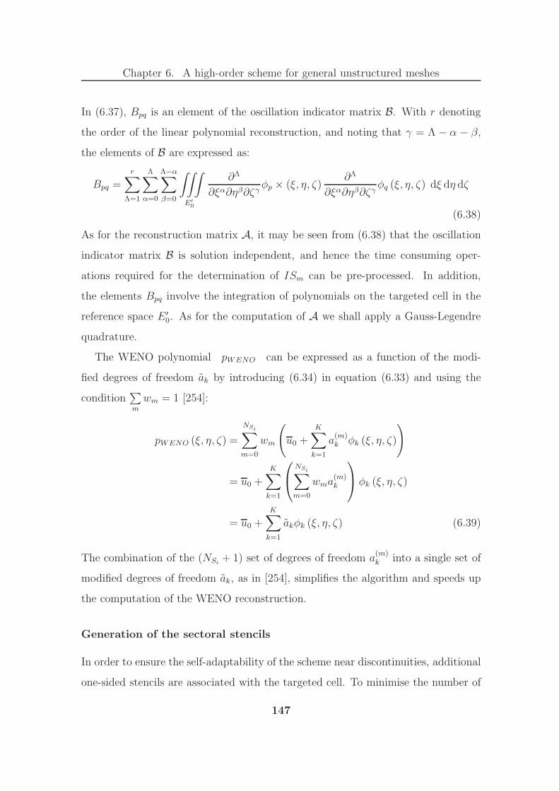
Chapter 6. A high-order scheme for general unstructured meshes
In (6.37), Bpq is an element of the oscillation indicator matrix B. With r denoting
the order of the linear polynomial reconstruction, and noting that γ = Λ − α − β,
the elements of B are expressed as:
Bpq =r∑
Λ=1
Λ∑
α=0
Λ−α∑
β=0
∫∫∫
E′
0
∂Λ
∂ξα∂ηβ∂ζγφp × (ξ, η, ζ)
∂Λ
∂ξα∂ηβ∂ζγφq (ξ, η, ζ) dξ dη dζ
(6.38)
As for the reconstruction matrix A, it may be seen from (6.38) that the oscillation
indicator matrix B is solution independent, and hence the time consuming oper-
ations required for the determination of ISm can be pre-processed. In addition,
the elements Bpq involve the integration of polynomials on the targeted cell in the
reference space E ′0. As for the computation of A we shall apply a Gauss-Legendre
quadrature.
The WENO polynomial pWENO can be expressed as a function of the modi-
fied degrees of freedom ak by introducing (6.34) in equation (6.33) and using the
condition∑m
wm = 1 [254]:
pWENO (ξ, η, ζ) =
NSi∑
m=0
wm
(
u0 +
K∑
k=1
a(m)k φk (ξ, η, ζ)
)
= u0 +
K∑
k=1
NSi∑
m=0
wma(m)k
φk (ξ, η, ζ)
= u0 +K∑
k=1
akφk (ξ, η, ζ) (6.39)
The combination of the (NSi+ 1) set of degrees of freedom a
(m)k into a single set of
modified degrees of freedom ak, as in [254], simplifies the algorithm and speeds up
the computation of the WENO reconstruction.
Generation of the sectoral stencils
In order to ensure the self-adaptability of the scheme near discontinuities, additional
one-sided stencils are associated with the targeted cell. To minimise the number of
147

Chapter 6. A high-order scheme for general unstructured meshes
stencils, Titarev et al. suggested the following guidelines [254]:
1. The stencils are disjoint (apart from the targeted cell).
2. The union of one-sided stencils covers the whole space surrounding the targeted
cell.
3. The stencils are compact. We improved the methodology reported in [254] by
choosing the stencils compact in the reference space ξ (see Section 6.3.1): i.e.
in a given sector of the physical space the stencil gathers the jmax elements
having the minimum centre-to-centre distance to the targeted cell in ξ.
As the mapping is trilinear, a given sector Sl of the physical space contains the
elements Ej — images of the elements E ′j under the mapping x = x (ξ, η, ζ) — such
that the inverse images E ′j are themselves contained in the sector of the reference
space S ′l, inverse image of Sl under x = x (ξ, η, ζ). Therefore gathering elements in
Sl for the stencil selection, is identical to gathering them in S ′l.
Definition of the sectors In order to remain as general as possible on a 3D
mixed-element unstructured mesh, we aim to take as many compact stencils as there
are internal faces FIl of the considered element E0 (i.e. faces of E0 that are not on
a domain boundary). For each face FIl, we choose to define the sector — in which
the stencil will be constructed — from the contour of FIl and the centre C0 of the
cell E0. As illustrated in Figure 6.7, the cells selected to form the sector stencil have
their centre in the portion of physical space:
• encompassing the centre of the face FIl.
• delimited by the surface of the cone Cl admitting C0 as apex and the contour
of FIl as directrix.
148
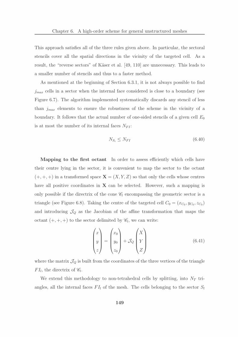
Chapter 6. A high-order scheme for general unstructured meshes
This approach satisfies all of the three rules given above. In particular, the sectoral
stencils cover all the spatial directions in the vicinity of the targeted cell. As a
result, the “reverse sectors” of Kaser et al. [49, 110] are unnecessary. This leads to
a smaller number of stencils and thus to a faster method.
As mentioned at the beginning of Section 6.3.1, it is not always possible to find
jmax cells in a sector when the internal face considered is close to a boundary (see
Figure 6.7). The algorithm implemented systematically discards any stencil of less
than jmax elements to ensure the robustness of the scheme in the vicinity of a
boundary. It follows that the actual number of one-sided stencils of a given cell E0
is at most the number of its internal faces NFI :
NSi≤ NFI (6.40)
Mapping to the first octant In order to assess efficiently which cells have
their centre lying in the sector, it is convenient to map the sector to the octant
(+,+,+) in a transformed space X = (X, Y, Z) so that only the cells whose centres
have all positive coordinates in X can be selected. However, such a mapping is
only possible if the directrix of the cone Cl encompassing the geometric sector is a
triangle (see Figure 6.8). Taking the centre of the targeted cell C0 = (xC0 , yC0, zC0)
and introducing JQ as the Jacobian of the affine transformation that maps the
octant (+,+,+) to the sector delimited by Cl, we can write:
x
y
z
=
x0
y0
z0
+ JQ
X
Y
Z
(6.41)
where the matrix JQ is built from the coordinates of the three vertices of the triangle
FIl, the directrix of Cl.
We extend this methodology to non-tetrahedral cells by splitting, into NT tri-
angles, all the internal faces FIl of the mesh. The cells belonging to the sector Sl
149

Chapter 6. A high-order scheme for general unstructured meshes
Figure 6.7: Ten-cells sectoral stencils of E0 coloured by sector; discarded stencil
hatched in grey; domain boundaries hatched in black — as produced by the fast
search procedure in 2D
delimited by Cl belong to the union of sub-sectors Sli delimited by the cones Cli
associated with the NT triangles:
Sl =
NT⋃
i=1
Sli (6.42)
The sub-sectors Sli are therefore successively mapped to the octant (+,+,+) and
for each potential stencil cell Ek, we produce and test a condition of inclusion of
its centre Ck (expressed in X(i): the transformed space associated to Sli) in the
various sub-sectors. Using the symbol∑
to indicate the repeated use of the logical
150

Chapter 6. A high-order scheme for general unstructured meshes
Figure 6.8: Mapping to the first octant (+,+,+)
disjunction, our condition reads:
Condk =
NT∑
i=1
(Ck ∈ Sli) (6.43)
=
NT∑
i=1
(pos
(X
(i)Ck
)× pos
(Y
(i)Ck
)× pos
(Z
(i)Ck
))(6.44)
where:
∀x ∈ R : pos (x) =
1 if x ≥ 0
0 if x < 0(6.45)
The above test guarantees that cells whose centres belong to several sub-sectors are
added just once to the list of sector members. It avoids the need for a cumbersome
and time-consuming iterative test against all the cells already identified as sector
members. In order to optimise the procedure, the internal faces are split into a
minimal number of triangles, such that NT = 1 for triangular faces (no split),
NT = 2 for quadrilateral faces and NT = number of sides for polygonal faces. As
this split of the internal faces is performed in any case during the tetrahedralisation
algorithm (see Section 6.3.1), the tetrahedral decomposition of the mesh is run prior
to the generation of the one-sided stencils.
151
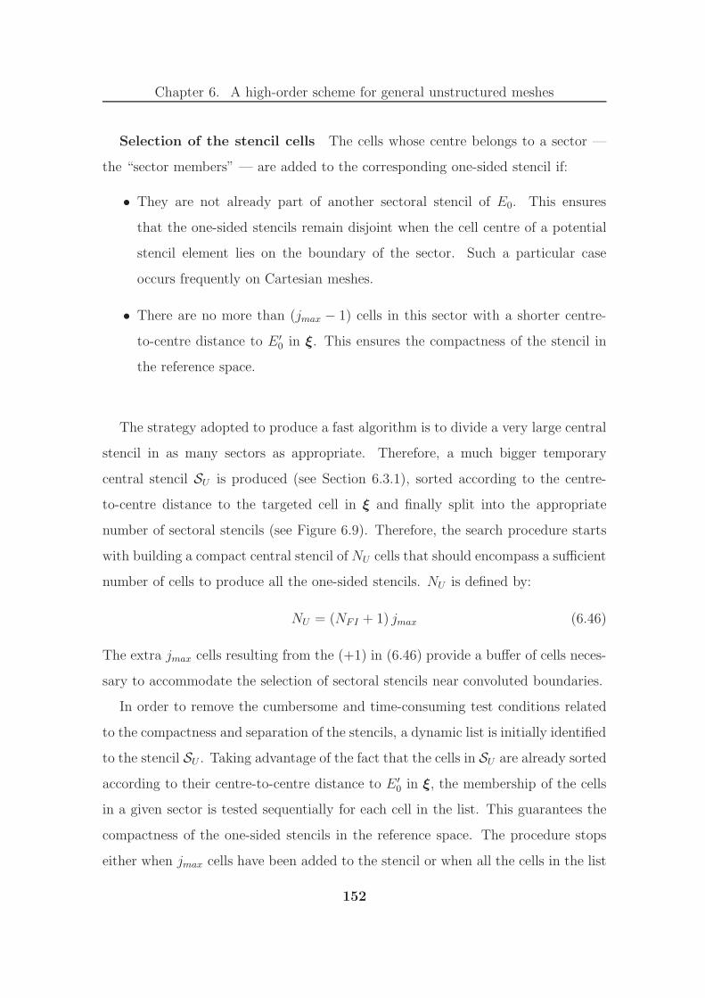
Chapter 6. A high-order scheme for general unstructured meshes
Selection of the stencil cells The cells whose centre belongs to a sector —
the “sector members” — are added to the corresponding one-sided stencil if:
• They are not already part of another sectoral stencil of E0. This ensures
that the one-sided stencils remain disjoint when the cell centre of a potential
stencil element lies on the boundary of the sector. Such a particular case
occurs frequently on Cartesian meshes.
• There are no more than (jmax − 1) cells in this sector with a shorter centre-
to-centre distance to E ′0 in ξ. This ensures the compactness of the stencil in
the reference space.
The strategy adopted to produce a fast algorithm is to divide a very large central
stencil in as many sectors as appropriate. Therefore, a much bigger temporary
central stencil SU is produced (see Section 6.3.1), sorted according to the centre-
to-centre distance to the targeted cell in ξ and finally split into the appropriate
number of sectoral stencils (see Figure 6.9). Therefore, the search procedure starts
with building a compact central stencil of NU cells that should encompass a sufficient
number of cells to produce all the one-sided stencils. NU is defined by:
NU = (NFI + 1) jmax (6.46)
The extra jmax cells resulting from the (+1) in (6.46) provide a buffer of cells neces-
sary to accommodate the selection of sectoral stencils near convoluted boundaries.
In order to remove the cumbersome and time-consuming test conditions related
to the compactness and separation of the stencils, a dynamic list is initially identified
to the stencil SU . Taking advantage of the fact that the cells in SU are already sorted
according to their centre-to-centre distance to E ′0 in ξ, the membership of the cells
in a given sector is tested sequentially for each cell in the list. This guarantees the
compactness of the one-sided stencils in the reference space. The procedure stops
either when jmax cells have been added to the stencil or when all the cells in the list
152

Chapter 6. A high-order scheme for general unstructured meshes
Figure 6.9: Thirteen-cells sectoral stencils of E0 coloured by sector: the coloured
thick lines indicate the progression of the search; discarded stencil hatched in grey;
domain boundaries hatched in black — as produced by the fast search procedure in
2D
have been tested. The condition requiring disjoint stencils is ensured by removing
the cells selected at each iteration. This fast search algorithm produces the best
dataset for an accurate reconstruction of the solution, as the remaining stencils are
very compact in ξ.
Determination of the oscillation indicator matrix
On a general unstructured mesh, the oscillation indicator matrix B is solution in-
dependent and therefore can be pre-processed. We have derived a computationally
153
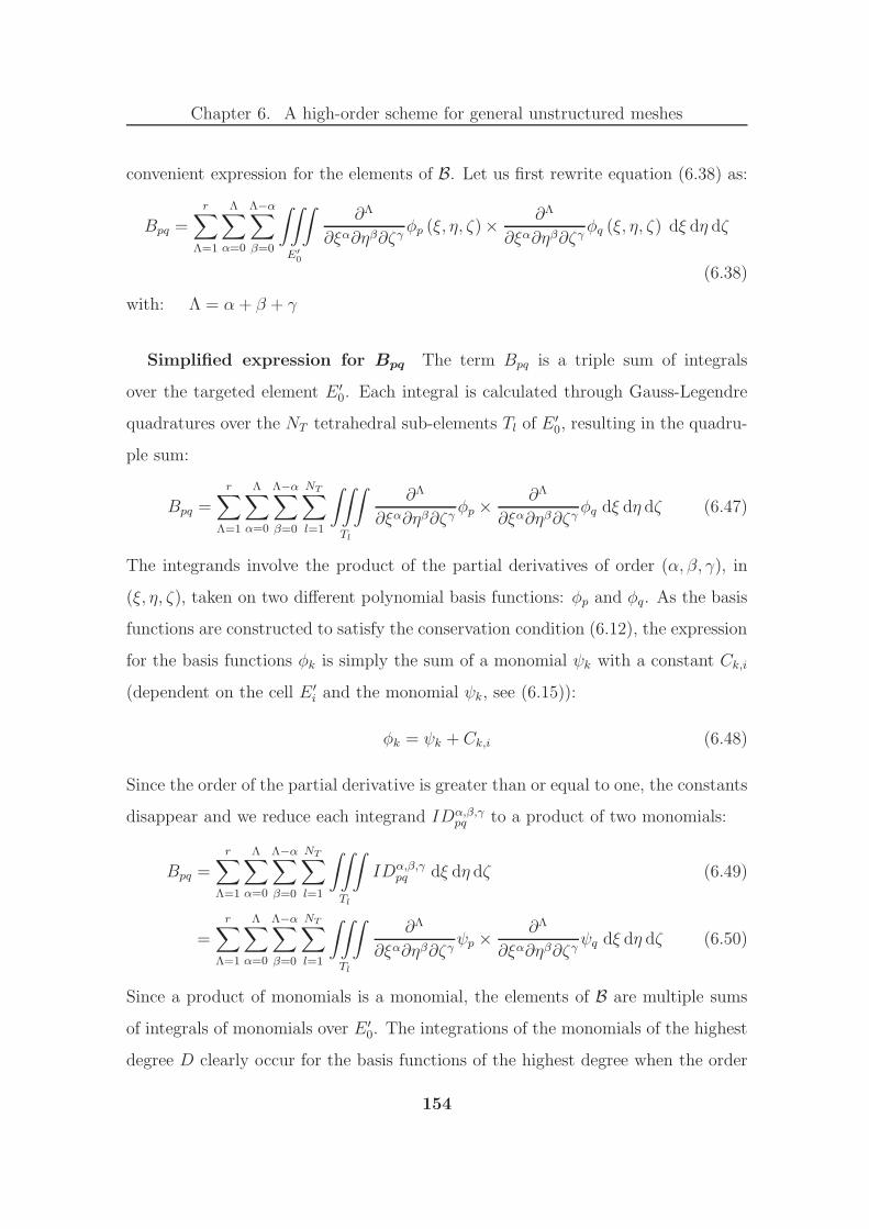
Chapter 6. A high-order scheme for general unstructured meshes
convenient expression for the elements of B. Let us first rewrite equation (6.38) as:
Bpq =
r∑
Λ=1
Λ∑
α=0
Λ−α∑
β=0
∫∫∫
E′
0
∂Λ
∂ξα∂ηβ∂ζγφp (ξ, η, ζ)× ∂Λ
∂ξα∂ηβ∂ζγφq (ξ, η, ζ) dξ dη dζ
(6.38)
with: Λ = α+ β + γ
Simplified expression for Bpq The term Bpq is a triple sum of integrals
over the targeted element E ′0. Each integral is calculated through Gauss-Legendre
quadratures over the NT tetrahedral sub-elements Tl of E ′0, resulting in the quadru-
ple sum:
Bpq =
r∑
Λ=1
Λ∑
α=0
Λ−α∑
β=0
NT∑
l=1
∫∫∫
Tl
∂Λ
∂ξα∂ηβ∂ζγφp ×
∂Λ
∂ξα∂ηβ∂ζγφq dξ dη dζ (6.47)
The integrands involve the product of the partial derivatives of order (α, β, γ), in
(ξ, η, ζ), taken on two different polynomial basis functions: φp and φq. As the basis
functions are constructed to satisfy the conservation condition (6.12), the expression
for the basis functions φk is simply the sum of a monomial ψk with a constant Ck,i
(dependent on the cell E ′i and the monomial ψk, see (6.15)):
φk = ψk + Ck,i (6.48)
Since the order of the partial derivative is greater than or equal to one, the constants
disappear and we reduce each integrand IDα,β,γpq to a product of two monomials:
Bpq =
r∑
Λ=1
Λ∑
α=0
Λ−α∑
β=0
NT∑
l=1
∫∫∫
Tl
IDα,β,γpq dξ dη dζ (6.49)
=r∑
Λ=1
Λ∑
α=0
Λ−α∑
β=0
NT∑
l=1
∫∫∫
Tl
∂Λ
∂ξα∂ηβ∂ζγψp ×
∂Λ
∂ξα∂ηβ∂ζγψq dξ dη dζ (6.50)
Since a product of monomials is a monomial, the elements of B are multiple sums
of integrals of monomials over E ′0. The integrations of the monomials of the highest
degree D clearly occur for the basis functions of the highest degree when the order
154

Chapter 6. A high-order scheme for general unstructured meshes
of the partial derivative is lowest: Λmin = 1. As a result, the highest degree D to
be considered is expressed by:
D = 2 (r − Λmin)
= 2r − 2 (6.51)
The associated number of non-constant monomials of degree less than or equal to
(2r − 2) is then:
KIS =r (4r2 − 1)
3− 1 (6.52)
Derivation of the integrands of Bpq Similarly to the determination of the
elements of A, the calculation of the Bpq involve a combination of integrals of mono-
mials. However, in the computations of B, the degree of the monomials to be inte-
grated reaches (2r − 2) and the integrations are only performed over the targeted
cell E ′0. In order to perform the integration, we express the integrand IDα,β,γ
pq as a
monomial. Introducing (A,B,C) ∈ J0, rK3 such that1 ≤ A+B+C ≤ r
, we can
express the monomial ψk (ξ, η, ζ) by:
ψk (ξ, η, ζ) = ξAηBζC (6.53)
Applying to ψk the partial derivative of order (α, β, γ), in (ξ, η, ζ), leads to:
∂Λ
∂ξα∂ηβ∂ζγ(ψk) = KDξ
(A−α)η(B−β)ζ (C−γ) (6.54)
where:
KD =
A !(A−α) !
× B !(B−β) !
× C !(C−γ) !
if (A ≥ α) ∩ (B ≥ β) ∩ (C ≥ γ)
0 otherwise(6.55)
KD can be expressed in a more convenient manner by using the function “pos”
introduced in Section 6.3.1:
KD = pos (A− α) × pos (B − β) × pos (C − γ) × A !(A−α) !
× B !(B−β) !
× C !(C−γ) !
(6.56)
155

Chapter 6. A high-order scheme for general unstructured meshes
Then, introducing: (A1, B1, C1, A2, B2, C2) ∈ J0, rK6 such that1 ≤ Ai + Bi +
Ci ≤ r , i = 1, 2
and making use of (6.56), we express the integrand IDα,β,γpq as a
monomial:
IDα,β,γpq = KEξ
(A1+A2−2α)η(B1+B2−2β)ζ (C1+C2−2γ) (6.57)
with:
KE = pos (A1 − α) × pos (B1 − β) × pos (C1 − γ) × A1 !(A1−α) !
× B1 !(B1−β) !
× C1 !(C1−γ) !
× pos (A2 − α) × pos (B2 − β) × pos (C2 − γ) × A2 !(A2−α) !
× B2 !(B2−β) !
× C2 !(C2−γ) !
(6.58)
Efficient computation of B By inserting (6.57) in (6.49) we derive the final
formulation for the elements Bpq:
Bpq =
r∑
Λ=1
Λ∑
α=0
Λ−α∑
β=0
NT∑
l=1
∫∫∫
Tl
KEξ(A1+A2−2α)η(B1+B2−2β)ζ (C1+C2−2γ) dξ dη dζ (6.59)
It may be noted that:
• The K integrals of monomials of degrees up to r are readily available from the
algorithm for computing the reconstruction matrix A.
• The calculation of the different matrix elements Bpq generally involves many
of the same monomial integrations over the targeted cell E ′0.
Therefore we choose to store the list of KIS integrals of monomials over E ′0 for each
cell of the mesh. The elements of B are then efficiently computed from this list of
integrals by applying the formula (6.59). It is worth noting that only the integrals
of monomials of degree higher than r have to be calculated, as the first K integrals
of the list have already been computed (see Section 6.3.1).
Calculation of the modified degrees of freedom
Since the modified degrees of freedom ak are a function of both the WENO weights
wm and the degrees of freedom a(m)k associated to the stencil Sm (see (6.39)), the
156

Chapter 6. A high-order scheme for general unstructured meshes
calculation of the ak is performed at run time. This computation takes the following
steps:
1. The generation of the vector of data bm for each stencil Sm of each cell of
the mesh. The components b(m)j are computed from the cell averages of the
solution u(m)j (t) in the cells of Sm at a given time t:
b(m)j = u
(m)j (t) − u
(m)0 (t) j = 1, · · · , jmax ; m = 0, · · · , NS (6.60)
2. The determination of the (NS + 1) vectors of degrees of freedom am from
the effective pseudo-inverses(A†τ
)(m)of the reconstruction matrices and the
vectors of data bm:
am =(A†τ
)(m)bm m = 0, · · · , NS (6.61)
3. For each stencil Sm, calculation of the smoothness indicator ISm from the
oscillation indicator matrix B and the vector of degrees of freedom am:
ISm = aTm (B am) m = 0, · · · , NS (6.62)
4. Calculation of the WENO weights wm from the smoothness indicators ISm
(see (6.37) and (6.38)).
5. For each cell of the mesh, calculation of the vector of modified degrees of
freedom a from the (NS + 1) vector of degrees of freedom am and the WENO
weights wm:
a =
NS∑
m=0
wmam (6.63)
6.3.3 Determination of the numerical flux
With the details of the polynomial reconstruction procedure in mind, let us derive
the flux calculation for the system of equations (6.1). This is a necessary step, since
some of the simplifications relevant to tetrahedral grids [49] and 2D mixed-element
157
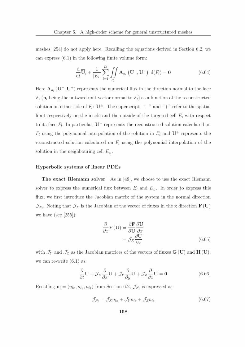
Chapter 6. A high-order scheme for general unstructured meshes
meshes [254] do not apply here. Recalling the equations derived in Section 6.2, we
can express (6.1) in the following finite volume form:
d
dtUi +
1
|Ei|Li∑
l=1
∫∫
Fl
Anl
(U−,U+
)d(Fl) = 0 (6.64)
Here Anl(U−,U+) represents the numerical flux in the direction normal to the face
Fl (nl being the outward unit vector normal to Fl) as a function of the reconstructed
solution on either side of Fl: U±. The superscripts “−” and “+” refer to the spatial
limit respectively on the inside and the outside of the targeted cell Ei with respect
to its face Fl. In particular, U− represents the reconstructed solution calculated on
Fl using the polynomial interpolation of the solution in Ei and U+ represents the
reconstructed solution calculated on Fl using the polynomial interpolation of the
solution in the neighbouring cell Ejl.
Hyperbolic systems of linear PDEs
The exact Riemann solver As in [49], we choose to use the exact Riemann
solver to express the numerical flux between Ei and Ejl. In order to express this
flux, we first introduce the Jacobian matrix of the system in the normal direction
JNl. Noting that JX is the Jacobian of the vector of fluxes in the x direction F (U)
we have (see [255]):
∂
∂xF (U) =
∂F
∂U
∂U
∂x
= JX∂U
∂x(6.65)
with JY and JZ as the Jacobian matrices of the vectors of fluxes G (U) and H (U),
we can re-write (6.1) as:
∂
∂tU + JX
∂
∂xU + JY
∂
∂yU + JZ
∂
∂zU = 0 (6.66)
Recalling nl = (nlx, nly, nlz) from Section 6.2, JNlis expressed as:
JNl= JXnlx + JY nly + JZnlz (6.67)
158

Chapter 6. A high-order scheme for general unstructured meshes
In order to express the numerical flux Anl, we introduce (after [255]) the diagonal
matrix of eigenvalues ΛNl= diag (λl1, λl2, · · · , λlP ) of JNl
and the left and right
eigenvector matrices: LNland RNl
, so that JNl= LNl
ΛNlRNl
. Defining the matrix
absolute value operator: |JNl| = LNl
|ΛNl|RNl
with |ΛNl| = diag (|λl1|, |λl2|, · · · , |λlP |),
the numerical flux — associated with the exact Riemann solver — between Ei and
Ejl becomes [49, 255]:
Anl
(U−,U+
)=
1
2
((JNl
+ |JNl|)U− + (JNl
− |JNl|)U+
)(6.68)
Computation of the numerical flux Introducing the expression (6.68) in
the finite volume formulation (6.64) leads to:
0 =d
dtUi +
1
|Ei|Li∑
l=1
1
2(JNl
+ |JNl|)∫∫
Fl
U− d(Fl)
+1
|Ei|Li∑
l=1
1
2(JNl
− |JNl|)∫∫
Fl
U+ d(Fl) (6.69)
Since the reconstruction procedure relies on a mapping to avoid introducing cum-
bersome scaling factors, the reconstruction is performed on a reference space ξ. As
a result, the polynomial representing the solution U is only known as a function of
ξ. Therefore, we relate the integrals in (6.69) to their counterparts over the faces
F ′l of E ′
i in the reference spaces ξ− and ξ+ associated respectively to E ′i and E ′
jl:
∫∫
Fl
U± d(Fl) =|Fl||F ′l |
∫∫
F ′
l
U±(ξ±, t
)d(F ′
l ) (6.70)
As the transformation from the physical space to the reference space is affine, the
ratio of square roots of the Gram determinants involved (see [117]) is constant and
may be taken out of the integrals.
In the case of a vector variable U, exactly the same basis functions φk are used for
the polynomial reconstruction of all the components up of U, since the functions φk
are only dependent on the mesh. As each component of the vector variable can be
159

Chapter 6. A high-order scheme for general unstructured meshes
considered as a scalar variable, a set of k modified degrees of freedom ak is calculated
at each time step for every scalar variable up. Therefore there are as many modified
degrees of freedom associated with φk as there are components in U, and these are
gathered in the vector ak.
Recalling the equation for the polynomial reconstruction of a scalar variable
(6.39), the formulae for U− (ξ−, t) and U+ (ξ+, t), at time t = n∆t, are:
U−(ξ−, t
)=(Ui
)(n)+
K∑
k=1
(ak)(n)i (φk)i
(ξ−)
U+(ξ+, t
)=(Ujl
)(n)+
K∑
k=1
(ak)(n)jl
(φk)jl(ξ+)
(6.71)
Replacing U− (ξ−, t) and U+ (ξ+, t) in (6.70) by their expressions in (6.71) leads to:
∫∫
Fl
U− d(Fl) = |Fl|(Ui
)(n)+
|Fl||F ′l |
K∑
k=1
((ak)
(n)i
∫∫
F ′
l
(φk)i(ξ−)
d(F ′l )
)
∫∫
Fl
U+ d(Fl) = |Fl|(Ujl
)(n)+
|Fl||F ′l |
K∑
k=1
((ak)
(n)jl
∫∫
F ′
l
(φk)jl(ξ+)
d(F ′l )
)
(6.72)
In (6.72), the integrals of the basis functions (φk)i (ξ−) and (φk)jl (ξ
+) are inde-
pendent of the solution U. Hence the integrals of the k basis functions (φk)i (ξ−)
are pre-computed for all the faces F ′l of all the transformed elements E ′
i. As a re-
sult, the integrals of (φk)i (ξ−) and (φk)jl (ξ
+) are readily available for the run-time
calculation of the inter-cell flux between any neighbouring cells.
Surface integrals of the basis functions Recalling that the basis functions
φk are constructed from the monomials ψk (see (6.13)), the expression for the kth
basis function of the element Ei: (φk)i is:
(φk)i = ψk −1
|E ′i|
∫∫∫
E′
i
ψk dξ dη dζ (6.73)
160

Chapter 6. A high-order scheme for general unstructured meshes
Therefore, the integral of the basis function (φk)i is expressed as:
∫∫
F ′
l
(φk)i(ξ−)
d(F ′l ) =
∫∫
F ′
l
ψk(ξ−)
d(F ′l ) −
|F ′l |
|E ′i|
∫∫∫
E′
i
ψk dξ dη dζ (6.74)
In (6.74), the triple integral of the monomials ψk over the volume E ′i is calculated
during the linear reconstruction (see Section 6.3.1) and is therefore readily available.
As in Section 6.3.1, in order to maximise the efficiency of the method, we choose to
calculate the surface integral of the monomial ψk over the face F ′l with a Gaussian
quadrature. Since the affine transformation of a convex polyhedral does not gen-
erally result in the standard domain required by Gauss-Legendre quadratures, we
take advantage of the tetrahedralisation of the mesh and, for each face F ′l , sum the
Gaussian quadratures produced for the NTltriangles T ′
lm constituting F ′l :
∫∫
F ′
l
ψk(ξ−)
d(F ′l ) =
NTl∑
m=1
∫∫
T ′
lm
ψk(ξ−)
d(T ′lm) (6.75)
Hyperbolic systems of non-linear PDEs
In the general case, the flux Anl(U−,U+) (see (6.64)) varies along the face Fl.
Consequently, as we perform the integration of the flux with a Gauss-Legendre
quadrature, Anl(U−,U+) is evaluated at each Gauss point xβ of each triangle Tlm
constituting the face Fl.
The solution being reconstructed in the mapped space, the integral of the flux
are calculated over the transformed face F ′l . Re-writing (6.64) with the integral
expressed over F ′l leads to:
d
dtUi +
1
|Ei|Li∑
l=1
|Fl||F ′l |
∫∫
F ′
l
Anl
(U−,U+
)d(F ′
l ) = 0 (6.76)
For each point of the Gaussian quadrature, the reconstructed solutions on either
side of the face, U−β and U+
β , are evaluated at the mapped Gauss point in their
respective transformed space: ξ−β and ξ+
β . Introducing the weights of the Gaussian
161

Chapter 6. A high-order scheme for general unstructured meshes
quadrature kβ and the Riemann solver A, the integral of the flux can be expressed
as follows:
∫∫
F ′
l
Anl
(U−,U+
)d(F ′
l ) =
NTl∑
m=1
∫∫
T ′
lm
Anl
(U−,U+
)d(F ′
l )
=
NTl∑
m=1
Nβ∑
β=1
kβA(U−β ,U
+β
)(6.77)
As suggested by the equations above, the integrals of the basis functions can no
longer be pre-processed when solving non-linear PDEs. However, the values of the
basis functions on each Gauss point can be pre-computed to save computational run
time.
6.4 Application to the level set equation
6.4.1 Finite volume formulation of the level set equation
The WENO scheme presented in the previous section is to be used in the transport
of the level set scalar function ϕ for application to multiphase flows. Introducing
the velocity u = (u, v, w), the transport equation for ϕ may be expressed as:
∂ϕ
∂t+ u · ∇ϕ = 0 (6.78)
Assuming an incompressible flow we have ∇u = 0, so that (6.78) can be re-written
as a hyperbolic conservation law:
∂ϕ
∂t+ ∇ · (ϕu) = 0 (6.79)
In terms of the coordinates (x, y, z), (6.79) becomes
∂ϕ
∂t+
∂
∂x(uϕ) +
∂
∂y(vϕ) +
∂
∂z(wϕ) = 0 (6.80)
162

Chapter 6. A high-order scheme for general unstructured meshes
Comparing equation (6.80) to equation (6.1) provides the equalities:
F (ϕ) = uϕ
G (ϕ) = vϕ
H (ϕ) = wϕ
=⇒
A = (F,G,H)
= (uϕ, vϕ, wϕ)
Anl(ϕ−, ϕ+) = A · nl
(6.81)
In (6.81), ϕ− represents the reconstructed level set function calculated on Fl using
polynomial interpolation of the solution in Ei, while ϕ+ represents the reconstructed
level set function calculated on Fl using polynomial interpolation of the solution in
the neighbouring cell Ejl.
From (6.81) and (6.64), we express the transport equation for the level set in the
finite volume form:
d
dtϕi +
1
|Ei|Li∑
l=1
∫∫
Fl
Anl
(ϕ−, ϕ+
)d(Fl) = 0 (6.82)
The normal component of the flux Anlfor the level set equation can be obtained by
expressing (6.78) in terms of the coordinates to give:
∂ϕ
∂t+ u
∂ϕ
∂x+ v
∂ϕ
∂y+ w
∂ϕ
∂z= 0 (6.83)
Identifying equation (6.83) with equation (6.66) provides the equalities:
JX = u
JY = v
JZ = w
=⇒
JNl= unlx + vnly + wnlz
= u · nl= unl
(6.84)
Using (6.84) in (6.68), the normal component of the flux may be expressed as:
Anl
(ϕ−, ϕ+
)=
1
2
((unl
+ |unl|)ϕ− + (unl
− |unl|)ϕ+
)(6.85)
6.4.2 The Riemann problem for the level set equation
Simple manipulations of (6.83) demonstrates its rotational invariance (see Chapter
3 of [255]) according to:
A · nl = (F,G,H) · nl = nlxF + nlyG+ nlzH = F (6.86)
163

Chapter 6. A high-order scheme for general unstructured meshes
where F is the flux vector expressed in the direction nl, the first axis of the rotated
Cartesian frame (nl, sl, tl). The expression for F is:
F = (u · nl)ϕ = unlϕ (6.87)
In our three-dimensional space, the rotated Cartesian frame is obtained by apply-
ing successively two rotations around the angles θl1 ∈ [0, 2π] and θl2 ∈ [0, π]. The
equation (6.86) is valid ∀ (θl1, θl2) ∈ [0, 2π]× [0, π] (see Figure 6.10 for an illustra-
tion in 2D). Since we are dealing with a single scalar equation, the rotation matrix
Tl (θl1, θl2) (see [20, 255]) and its inverse both reduce to the scalar unity. From (6.81)
and (6.82), the finite volume formulation of (6.83) can be expressed as:
d
dtϕi +
1
|Ei|Li∑
l=1
∫∫
Fl
(F,G,H) · nl d(Fl) = 0 (6.88)
Figure 6.10: Rotated Cartesian frame in 2D: (nl, sl) — the first axis nl is orthogonal
to the arbitrary boundary ∂Ei of the control volume Ei
Using the rotational invariance of (6.83) we re-write (6.88) in the rotated Cartesian
frame (nl, sl, tl), where the direction nl is normal to the inter-cell boundary Fl.
Noting F , G and H , the flux vectors respectively in the directions nl, sl and tl, we
164
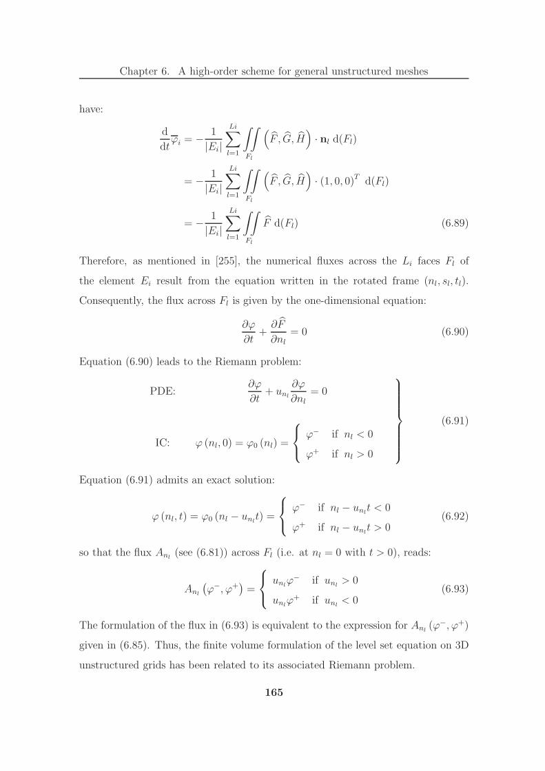
Chapter 6. A high-order scheme for general unstructured meshes
have:
d
dtϕi = − 1
|Ei|Li∑
l=1
∫∫
Fl
(F , G, H
)· nl d(Fl)
= − 1
|Ei|Li∑
l=1
∫∫
Fl
(F , G, H
)· (1, 0, 0)T d(Fl)
= − 1
|Ei|Li∑
l=1
∫∫
Fl
F d(Fl) (6.89)
Therefore, as mentioned in [255], the numerical fluxes across the Li faces Fl of
the element Ei result from the equation written in the rotated frame (nl, sl, tl).
Consequently, the flux across Fl is given by the one-dimensional equation:
∂ϕ
∂t+∂F
∂nl= 0 (6.90)
Equation (6.90) leads to the Riemann problem:
PDE:∂ϕ
∂t+ unl
∂ϕ
∂nl= 0
IC: ϕ (nl, 0) = ϕ0 (nl) =
ϕ− if nl < 0
ϕ+ if nl > 0
(6.91)
Equation (6.91) admits an exact solution:
ϕ (nl, t) = ϕ0 (nl − unlt) =
ϕ− if nl − unl
t < 0
ϕ+ if nl − unlt > 0
(6.92)
so that the flux Anl(see (6.81)) across Fl (i.e. at nl = 0 with t > 0), reads:
Anl
(ϕ−, ϕ+
)=
unl
ϕ− if unl> 0
unlϕ+ if unl
< 0(6.93)
The formulation of the flux in (6.93) is equivalent to the expression for Anl(ϕ−, ϕ+)
given in (6.85). Thus, the finite volume formulation of the level set equation on 3D
unstructured grids has been related to its associated Riemann problem.
165
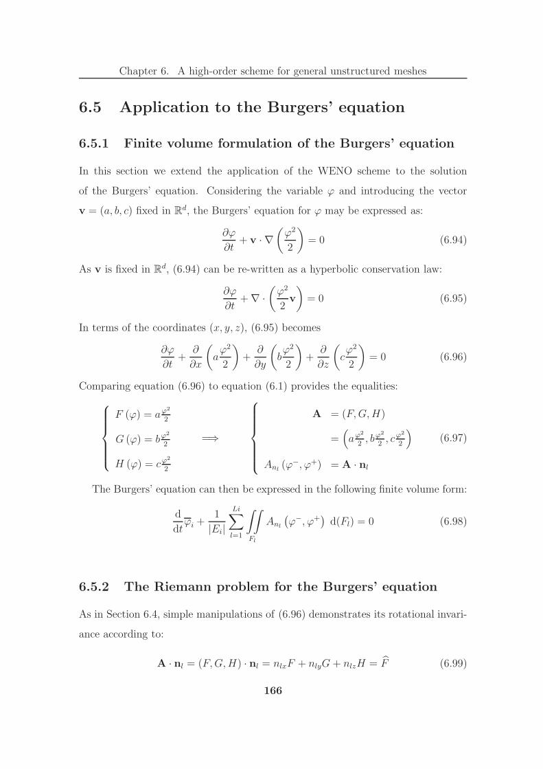
Chapter 6. A high-order scheme for general unstructured meshes
6.5 Application to the Burgers’ equation
6.5.1 Finite volume formulation of the Burgers’ equation
In this section we extend the application of the WENO scheme to the solution
of the Burgers’ equation. Considering the variable ϕ and introducing the vector
v = (a, b, c) fixed in Rd, the Burgers’ equation for ϕ may be expressed as:
∂ϕ
∂t+ v · ∇
(ϕ2
2
)= 0 (6.94)
As v is fixed in Rd, (6.94) can be re-written as a hyperbolic conservation law:
∂ϕ
∂t+ ∇ ·
(ϕ2
2v
)= 0 (6.95)
In terms of the coordinates (x, y, z), (6.95) becomes
∂ϕ
∂t+
∂
∂x
(aϕ2
2
)+
∂
∂y
(bϕ2
2
)+
∂
∂z
(cϕ2
2
)= 0 (6.96)
Comparing equation (6.96) to equation (6.1) provides the equalities:
F (ϕ) = aϕ2
2
G (ϕ) = bϕ2
2
H (ϕ) = cϕ2
2
=⇒
A = (F,G,H)
=(aϕ
2
2, bϕ
2
2, cϕ
2
2
)
Anl(ϕ−, ϕ+) = A · nl
(6.97)
The Burgers’ equation can then be expressed in the following finite volume form:
d
dtϕi +
1
|Ei|Li∑
l=1
∫∫
Fl
Anl
(ϕ−, ϕ+
)d(Fl) = 0 (6.98)
6.5.2 The Riemann problem for the Burgers’ equation
As in Section 6.4, simple manipulations of (6.96) demonstrates its rotational invari-
ance according to:
A · nl = (F,G,H) · nl = nlxF + nlyG+ nlzH = F (6.99)
166

Chapter 6. A high-order scheme for general unstructured meshes
where F is the flux vector expressed in the direction nl, the first axis of the rotated
Cartesian frame (nl, sl, tl). The expression for F is:
F = (v · nl)ϕ2
2= vnl
ϕ2
2(6.100)
Therefore, the flux across Fl is given by the one-dimensional equation:
∂ϕ
∂t+∂F
∂nl= 0 (6.101)
Equation (6.101) leads to the Riemann problem:
PDE:∂ϕ
∂t+
∂
∂nl
(vnl
ϕ2
2
)= 0
IC: ϕ (nl, 0) = ϕ0 (nl) =
ϕ− if nl < 0
ϕ+ if nl > 0
(6.102)
For the PDE (6.102), the characteristic speed λ (ϕ) is given by:
λ (ϕ) =dF
dϕ= vnl
ϕ (6.103)
Equation (6.102) admits an exact solution:
If λ (ϕ−) > λ (ϕ+) : ϕ (nl, t) =
ϕ− if nl − St < 0
ϕ+ if nl − St > 0
with: S = ∆ bF∆ϕ
=vnl
2(ϕ− + ϕ+)
If λ (ϕ−) ≤ λ (ϕ+) :
ϕ (nl, t) = ϕ− if nl
t≤ λ (ϕ−)
λ (ϕ) = nl
tif λ (ϕ−) < nl
t< λ (ϕ+)
ϕ (nl, t) = ϕ+ if nl
t≥ λ (ϕ+)
(6.104)
167
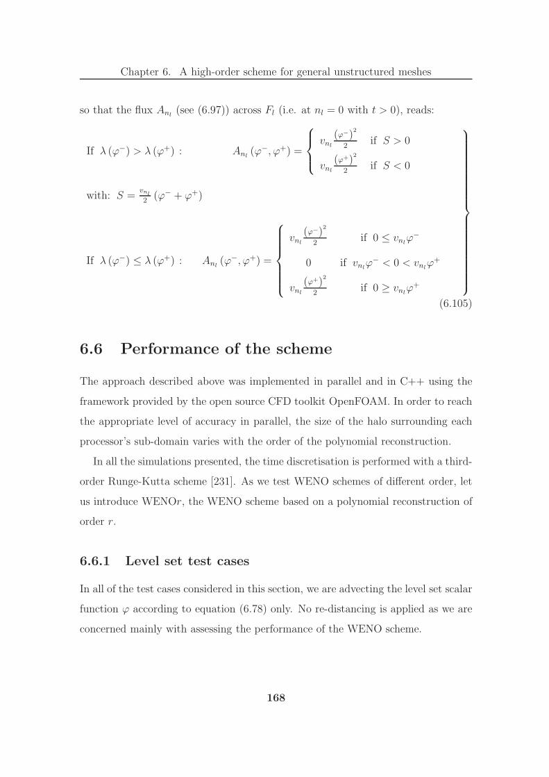
Chapter 6. A high-order scheme for general unstructured meshes
so that the flux Anl(see (6.97)) across Fl (i.e. at nl = 0 with t > 0), reads:
If λ (ϕ−) > λ (ϕ+) : Anl(ϕ−, ϕ+) =
vnl
(ϕ−)2
2if S > 0
vnl
(ϕ+)2
2if S < 0
with: S =vnl
2(ϕ− + ϕ+)
If λ (ϕ−) ≤ λ (ϕ+) : Anl(ϕ−, ϕ+) =
vnl
(ϕ−)2
2if 0 ≤ vnl
ϕ−
0 if vnlϕ− < 0 < vnl
ϕ+
vnl
(ϕ+)2
2if 0 ≥ vnl
ϕ+
(6.105)
6.6 Performance of the scheme
The approach described above was implemented in parallel and in C++ using the
framework provided by the open source CFD toolkit OpenFOAM. In order to reach
the appropriate level of accuracy in parallel, the size of the halo surrounding each
processor’s sub-domain varies with the order of the polynomial reconstruction.
In all the simulations presented, the time discretisation is performed with a third-
order Runge-Kutta scheme [231]. As we test WENO schemes of different order, let
us introduce WENOr, the WENO scheme based on a polynomial reconstruction of
order r.
6.6.1 Level set test cases
In all of the test cases considered in this section, we are advecting the level set scalar
function ϕ according to equation (6.78) only. No re-distancing is applied as we are
concerned mainly with assessing the performance of the WENO scheme.
168
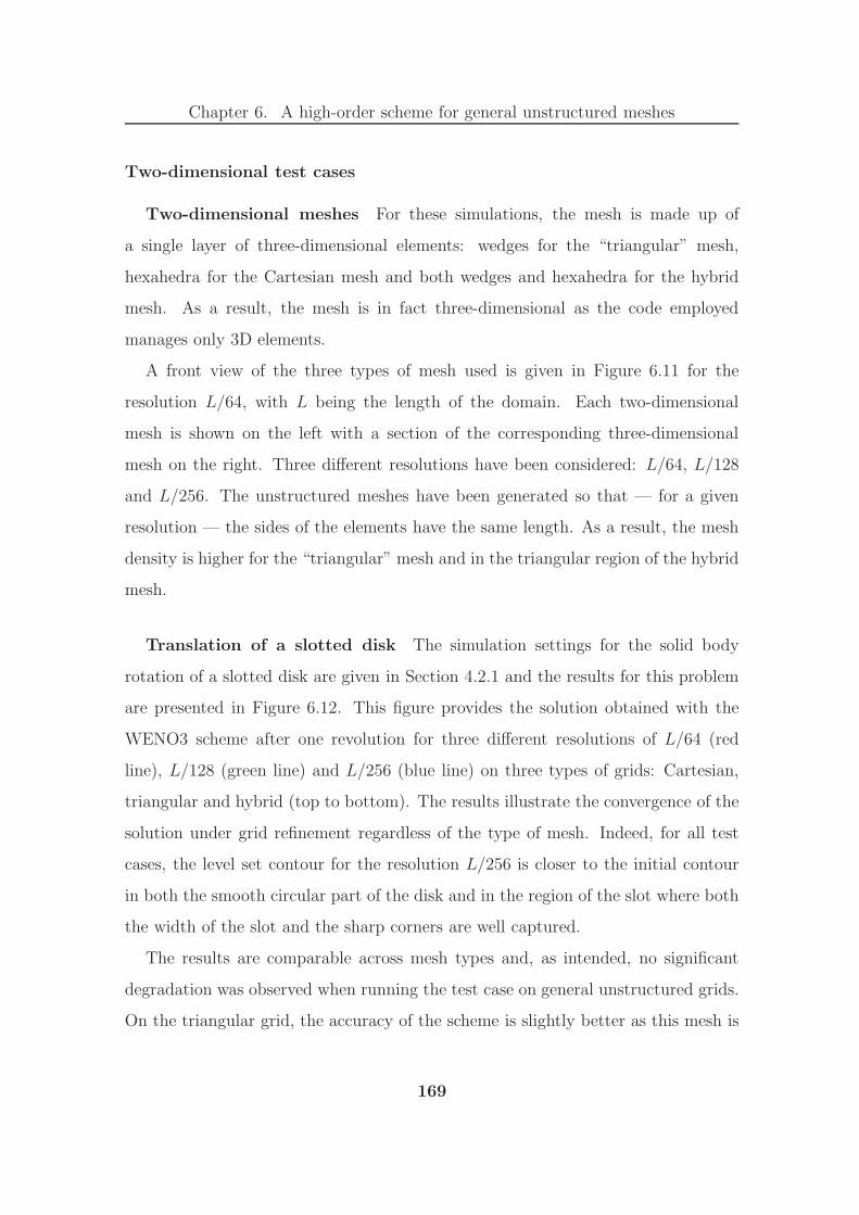
Chapter 6. A high-order scheme for general unstructured meshes
Two-dimensional test cases
Two-dimensional meshes For these simulations, the mesh is made up of
a single layer of three-dimensional elements: wedges for the “triangular” mesh,
hexahedra for the Cartesian mesh and both wedges and hexahedra for the hybrid
mesh. As a result, the mesh is in fact three-dimensional as the code employed
manages only 3D elements.
A front view of the three types of mesh used is given in Figure 6.11 for the
resolution L/64, with L being the length of the domain. Each two-dimensional
mesh is shown on the left with a section of the corresponding three-dimensional
mesh on the right. Three different resolutions have been considered: L/64, L/128
and L/256. The unstructured meshes have been generated so that — for a given
resolution — the sides of the elements have the same length. As a result, the mesh
density is higher for the “triangular” mesh and in the triangular region of the hybrid
mesh.
Translation of a slotted disk The simulation settings for the solid body
rotation of a slotted disk are given in Section 4.2.1 and the results for this problem
are presented in Figure 6.12. This figure provides the solution obtained with the
WENO3 scheme after one revolution for three different resolutions of L/64 (red
line), L/128 (green line) and L/256 (blue line) on three types of grids: Cartesian,
triangular and hybrid (top to bottom). The results illustrate the convergence of the
solution under grid refinement regardless of the type of mesh. Indeed, for all test
cases, the level set contour for the resolution L/256 is closer to the initial contour
in both the smooth circular part of the disk and in the region of the slot where both
the width of the slot and the sharp corners are well captured.
The results are comparable across mesh types and, as intended, no significant
degradation was observed when running the test case on general unstructured grids.
On the triangular grid, the accuracy of the scheme is slightly better as this mesh is
169

Chapter 6. A high-order scheme for general unstructured meshes
characterised by a higher density of elements for the same edge length.
Disk in a deformation field The simulation settings for the disk in the defor-
mation field are given in Section 4.2.1 and the results for this problem are presented
in Figure 6.12. This figure provides the solution obtained with the WENO3 scheme
at t = 3s for three different resolutions of L/64 (red line), L/128 (green line) and
L/256 (blue line) on three types of grids: Cartesian, triangular and hybrid (top
to bottom). The solution obtained with the WENO3 scheme on the triangular
grid (highest mesh density) of resolution L/256 has been taken as the reference case
(black line), as it provides the results closest to the “exact solution” as obtained with
the marker particle method by Rider and Kothe [201] or with the hybrid particle
level set method by Enright et al. [53].
For all test cases, under grid refinement the scheme demonstrates a greater ability
to capture thin ligaments, regardless of the type of mesh. Indeed, when the mesh
resolution is increased, the tail of the spiral becomes systematically longer. As with
the previous test case, no significant degradation of the results were observed on
general unstructured grids. It is worth also noting that the results obtained with
this WENO3 scheme without re-distancing compare very well with existing methods
that use WENO schemes of order five together with re-distancing (see [37, 246]).
NB: In order to compare the performance of the scheme with the work of previous
authors, the above two-dimensional test cases have been run with typical set-
tings. However, the comparison of the zero level set computed at a later time
should further differentiate the high-order schemes from the low-order ones [3].
170

Chapter 6. A high-order scheme for general unstructured meshes
Cartesian meshes
4096 cells (hexes) 262144 cells (hexes)
Triangular (left) and tetrahedral (right) meshes
9192 cells (wedges) 250704 cells (tets)
Hybrid meshes
7976 cells (hexes & wedges) 234843 cells (hexes, pyramids & tets)
Figure 6.11: Meshes for the level set 2D (left column) and 3D (right column) test
cases
171

Chapter 6. A high-order scheme for general unstructured meshes
Cartesian mesh
Triangular mesh
Hybrid mesh
Figure 6.12: Zero level set for the translation of a slotted disk (left column) and the
disk in a deformation field (right column) — In black: the reference; in red: solution
for L/64; in green: solution for L/128; in blue: solution for L/256
172

Chapter 6. A high-order scheme for general unstructured meshes
Three-dimensional test case
Three-dimensional meshes For the three-dimensional test case, the meshes
have been designed to maintain similar mesh density on the three types of mesh
considered (see Figure 6.11, right column, top to bottom): Cartesian mesh (262144
hexes), tetrahedral mesh (250704 tets) and hybrid mesh (234843 elements). With
such meshes, we extend our comparison of the performance of the scheme to 3D
Cartesian grids and unstructured meshes.
Sphere in a deformation field LeVeque extended the case presented in Sec-
tion 6.6.1 (see [125]) by considering a sphere in a three-dimensional deformation
field given by:
u (x, y, z) = 2 · sin2 (πx) · sin (2πy) · sin (2πz)
v (x, y, z) = − sin (2πx) · sin2 (πy) · sin (2πz)
w (x, y, z) = − sin (2πx) · sin (2πy) · sin2 (πz)
(6.106)
In this test, the domain is delimited by the points (0; 0; 0) and (1; 1; 1) and the
simulation follows a sphere of radius 0.15, centred on (0.35; 0.35; 0.35). The results
obtained with the WENO3 scheme for the sphere in the deformation field are given
in Figure 6.13. This figure provides the initial level set field (top row) together
with the solution obtained at t = 0.3125s (middle row) and t = 0.625s (bottom
row) on the three types of grids considered: Cartesian (left), tetrahedral (middle)
and hybrid (right). Therefore, this test case demonstrates the numerical scheme
on three-dimensional meshes. It also provides a means to assess the comparative
performance of the scheme on various types of 3D mesh.
As for the two-dimensional test cases, the results are comparable for all three
types of mesh. The results obtained on the Cartesian mesh are slightly better in
terms of smoothness. However, it is worth noting that the Cartesian mesh contains
more elements than the tetrahedral mesh (by 5%) and the hybrid mesh (by 12%). It
is clear from the results that the present approach works well on fully 3D structured,
173

Chapter 6. A high-order scheme for general unstructured meshes
unstructured and mixed-element meshes.
174

Chapter 6. A high-order scheme for general unstructured meshes
t = 0s
t = 0.3125s
t = 0.625s
Figure 6.13: Zero level set for the sphere in a deformation field on a Cartesian mesh
(left column), a tetrahedral mesh (middle column) and a hybrid mesh (right column)
— Time t = 0s, 0.3125s, 0.625s
175

Chapter 6. A high-order scheme for general unstructured meshes
6.6.2 Numerical convergence study
As in [286], we have chosen to demonstrate the numerical convergence of the WENO
scheme on the advection of a sine function. The scalar field is transported in a cube
with periodic boundary conditions, such that the solution at t = 1 should match
the initial field. The linear equation solved and the initial field are given below:
∂u∂t
+ 2∂u∂x
+ 2∂u∂y
+ 2∂u∂z
= 0, (x, y, z) ∈ [−1; 1]3
u (x, y, z, 0) = sin (π (x+ y + z)) + sin (2π (x+ y + z))(6.107)
We have solved this equation using both WENO3 and WENO4 schemes on Carte-
sian, tetrahedral and hybrid meshes. Three different level of refinement have been
considered for this study. Similarly to the 3D meshes in Section 6.6.1, the unstruc-
tured meshes have been generated so that — for a given resolution — the different
types of mesh have roughly the same number of elements.
The results of the numerical convergence study are presented in tables 6.1 to
6.3. These tables provide the numerical error in the L1 and L2 norms and their
associated convergence rates calculated using the number of cells Nc in the domain.
Introducing the error in the Lp norm ELp and the level of grid refinement k, the
formula for the order O(k)Lp reads:
O(k)Lp =
ln
(E
(k−1)Lp
E(k)Lp
)
ln
(3
√N
(k)c
N(k−1)c
) (6.108)
Although the numerical convergence study is only based on three levels of refine-
ment, the results illustrate that both WENO3 and WENO4 seem to systematically
reach a convergence rate significantly higher than the order r of their respective
polynomial interpolations. As in [49], we even observe that the order reached by the
WENO schemes tends to r+1 regardless of the type of mesh. A more comprehensive
convergence study should confirm the trends observed.
In the case of the WENO4 scheme and for the maximum level of resolution
considered, the full order of r+ 1 is not yet reached when calculating the error with
176

Chapter 6. A high-order scheme for general unstructured meshes
the L2 norm. However, the convergence rate seems to increase much faster for the
WENO4 scheme as the mesh is refined. A similar apparent loss of relative accuracy
has been observed by Pilliod and Puckett [178] with high-order schemes on coarse
grids. This phenomenon could also be due to the methodology employed to refine
the mesh [3]. Indeed, in [49] Dumbser et al. refined their tetrahedral meshes by
splitting the elements of the coarse mesh. As this methodology can be cumbersome
for mixed-element meshes, it has not been applied in this study.
Table 6.1: Numerical convergence study for the Cartesian meshes — Error and
associated order given for both WENO3 and WENO4
Scheme Number of cells EL1 OL1 EL2 OL2
WENO3 4096 4.8322 × 10⁻¹ — 5.321 × 10⁻¹ —
32768 3.5328 × 10⁻² 3.77 3.9349 × 10⁻² 3.76
262144 2.7226 × 10⁻³ 3.70 3.1798 × 10⁻³ 3.63
WENO4 4096 5.5752 × 10⁻¹ — 6.0496 × 10⁻¹ —
32768 5.4309 × 10⁻² 3.36 6.1376 × 10⁻² 3.3
262144 1.8432 × 10⁻³ 4.88 3.2140 × 10⁻³ 4.26
A plot of the error in the L2 norm against the normalised computational time
is given for both the WENO3 and the WENO4 scheme in figures 6.14 and 6.15
respectively. These graphs illustrate once again that the convergence rates reached
by the WENO schemes are independent of the type of grid.
It is interesting to note that figures 6.14 and 6.15 also suggest that — when
applying the WENO schemes to the transport of a smooth field — the tetrahedral
grids are more computationally efficient than the hybrid and Cartesian grids. This
can be explained by the considering the number of side stencils per element and the
linear weight given to the side stencils (see Section 6.2). The WENO reconstruction
method attributes to an element as many side stencils as it has faces. As a result,
177

Chapter 6. A high-order scheme for general unstructured meshes
Table 6.2: Numerical convergence study for the tetrahedral meshes — Error and
associated order given for both WENO3 and WENO4
Scheme Number of cells EL1 OL1 EL2 OL2
WENO3 3511 4.5490 × 10⁻¹ — 5.1014 × 10⁻¹ —
27983 3.1000 × 10⁻² 3.88 3.5946 × 10⁻² 3.83
251906 1.7644 × 10⁻³ 3.91 2.4047 × 10⁻³ 3.69
WENO4 3511 5.2429 × 10⁻¹ — 5.8559 × 10⁻¹ —
27983 5.2578 × 10⁻² 3.32 5.8891 × 10⁻² 3.32
251906 1.8486 × 10⁻³ 4.57 2.5985 × 10⁻³ 4.26
for a given number of cells, the Cartesian mesh would involve more side stencils per
element than the tetrahedral mesh. The average number of side stencil per element
of the hybrid mesh (as constructed in figure 6.11) would lie in between the two.
Therefore, the Cartesian mesh requires the largest amount of CPU time followed by
the hybrid mesh and then by the tetrahedral mesh. As we chose to give much smaller
linear weights to the side stencils than to the central stencil (see Section 6.2), for
smooth solutions, the contribution of the additional side stencils to the accuracy of
the calculation is not sufficient to offset the additional computational cost incurred.
178

Chapter 6. A high-order scheme for general unstructured meshes
Table 6.3: Numerical convergence study for the hybrid meshes — Error and associ-
ated order given for both WENO3 and WENO4
Scheme Number of cells EL1 OL1 EL2 OL2
WENO3 2945 5.6115 × 10⁻¹ — 6.2401 × 10⁻¹ —
27234 6.5903 × 10⁻² 2.89 8.8502 × 10⁻² 2.63
201293 4.4836 × 10⁻³ 4.03 6.1391 × 10⁻³ 4.00
WENO4 2945 5.8506 × 10⁻¹ — 6.5202 × 10⁻¹ —
27234 9.5779 × 10⁻² 2.44 1.2464 × 10⁻¹ 2.23
201293 5.4088 × 10⁻³ 4.31 7.7781 × 10⁻³ 4.16
Figure 6.14: L2 error vs. normalised CPU time for the WENO3 applied to the linear
equation
179

Chapter 6. A high-order scheme for general unstructured meshes
Figure 6.15: L2 error vs. normalised CPU time for the WENO4 applied to the linear
equation
180

Chapter 6. A high-order scheme for general unstructured meshes
6.6.3 Extension to a non-linear PDE
In order to demonstrate the capability of the WENO scheme on a non-linear PDE,
we choose to solve the 3D Burgers’ equation on a hybrid mesh of 1.73 × 10⁶ cells.
The equation is solved with the WENO3 scheme in a cubical domain with periodic
boundary conditions. We use the same initial condition as in [286], such that the
shock occurs at time t = 5π2 . The settings of the simulation are given below:
∂u∂t
+ ∂∂x
(u2
2
)+ ∂
∂y
(u2
2
)+ ∂
∂z
(u2
2
)= 0, (x, y, z) ∈ [−3; 3]3
u (x, y, z, 0) = 0.3 + 0.7 sin(π3
(x+ y + z))
(6.109)
The results of the calculation are given in Figure 6.16. A contour plot of the
solution on the surface of the domain is shown in the top left corner of Figure 6.16.
In the top right corner, we show a contour plot of the solution on the cut at z = 0.
Finally, in the bottom part of the figure, we compare the numerical solution to the
exact solution along the line x = y in the plane z = 0.
As intended, the scheme resolves the shock sharply with no trace of oscillatory
behaviour. In addition, as suggested by the bottom picture of Figure 6.16, the
numerical solution matches very well the exact solution all along the line considered.
181
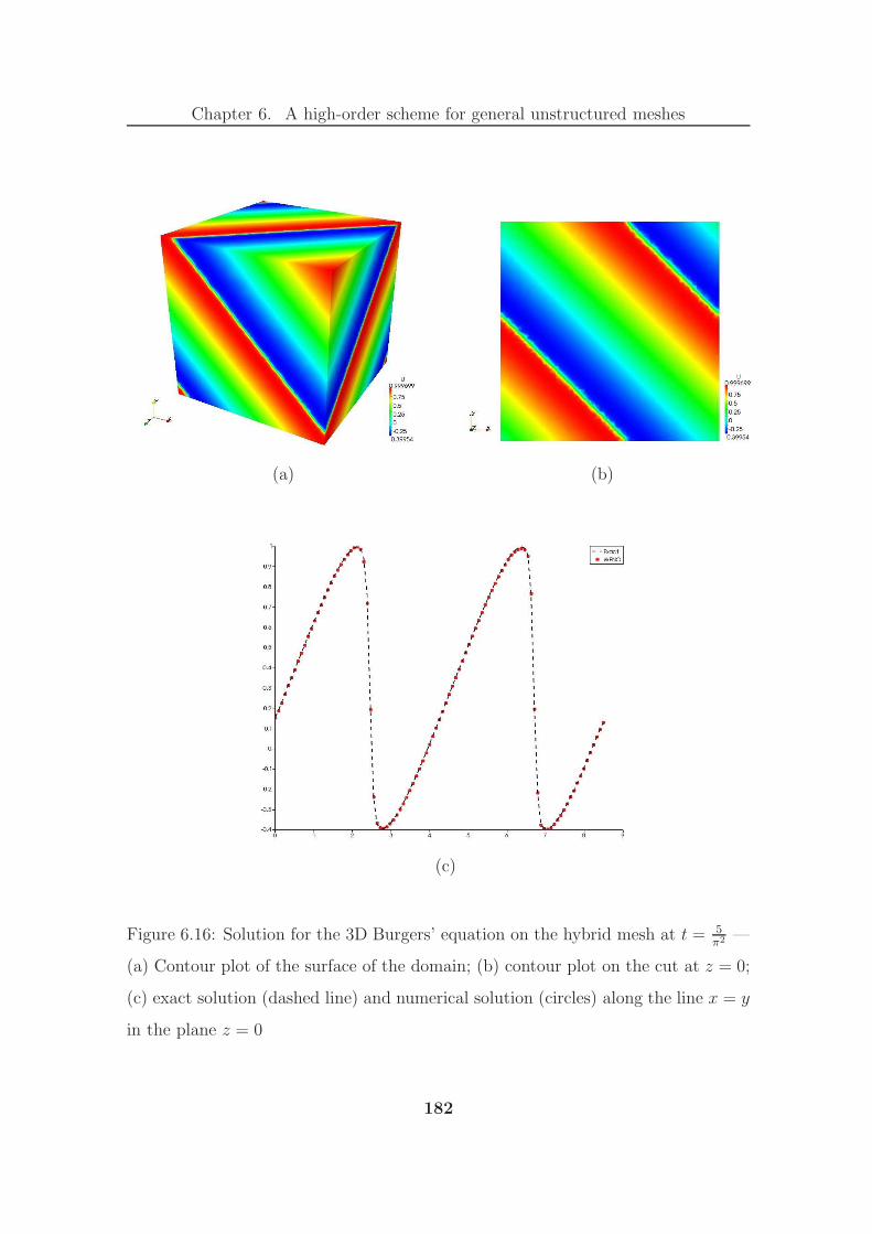
Chapter 6. A high-order scheme for general unstructured meshes
(a) (b)
(c)
Figure 6.16: Solution for the 3D Burgers’ equation on the hybrid mesh at t = 5π2 —
(a) Contour plot of the surface of the domain; (b) contour plot on the cut at z = 0;
(c) exact solution (dashed line) and numerical solution (circles) along the line x = y
in the plane z = 0
182
Chapter 7
Robust conservative level set
method
The method developed is based on the conservative level set method (CLS) of Olsson
et al. [164]. This is partly because this method generally offers a better trade-off
between mass conservation and computational cost than other interface description
methods — including state-of-the-art coupled level set-VOF (see for example [152]).
In addition, the method can be considered as mature, as it has been successfully
applied to the simulation of round liquid jet atomisation by Desjardins et al. [47].
Therefore, the risk associated with implementing and improving such a method is
low.
This chapter first provides a brief overview of the robust conservative level set
method and then describes the main building blocks of this interface-capturing tech-
nique. In particular, the transport of the level set scalar is detailed in Section 7.2,
the calculation of the interface normal is presented in Section 7.3 and the flux lim-
iter algorithm is explained in Section 7.4. Finally, the performance of the method
is assessed in Section 7.5.
183
Chapter 7. Robust conservative level set method
7.1 Overview of the method
As for the CLS method, the level set field transported, ϕ, can be initialised as a
hyperbolic tangent profile of the signed distance function from the interface (φ).
Introducing ǫ, a coefficient controlling the thickness of the interface, the field ϕ
reads:
ϕ =1
2
(1 + tanh
(φ
2ǫ
))(7.1)
With such a definition for the level set field ϕ, the phase boundary is located at
ϕ = 12. Although the hyperbolic tangent profile localises the phase transition in the
close vicinity of the interface, ϕ only tends to zero or one, at an infinite distance
in, respectively, the gas phase or the liquid phase. To mitigate this issue, the solver
as designed also offers the opportunity to set the initial field as the following sine
profile:
ϕ =
0 if φ < −ǫ1
2+φ
2ǫ+
1
2πsin
(πφ
ǫ
)if − ǫ ≤ φ ≤ ǫ
1 if φ > ǫ
(7.2)
The profile given in (7.2), will guarantee that the transition region will not be
bigger than 2ǫ.
As in [163, 164], the level set field ϕ represents the liquid volume fraction and we
are taking advantage of the constant thickness of the interface to apply the surface
tension via the continuum surface force method. As a result the material properties
are given by:
ϕ =
ρ = ρgas + (ρliq − ρgas)ϕ
µ = µgas + (µliq − µgas)ϕ(7.3)
As the interface is of constant thickness, this method is analogue to a phase field
method (see for example [100]). Therefore, it offers the possibility to implement
additional equations to describe the interface behaviour on a mesoscopic scale.
The robust conservative level set method (RCLS) that we have developed for
finite volume general unstructured meshes operates in three steps:
184

Chapter 7. Robust conservative level set method
1. Advection of the liquid volume fraction ϕ.
2. Re-initialisation of the level set field to maintain the interface thickness con-
stant.
3. Adjustment of the flux of liquid volume fraction to maintain boundedness.
The steps 1 and 2 are described in Section 7.2, and the third step is presented in
Section 7.4. The calculation of the interface normal, required by the re-initialisation
step, is detailed in Section 7.3.
7.2 Transport of the level set
7.2.1 Mathematical formulation
In the general case, the transport of the liquid volume fraction ϕ can be expressed
by the equation (7.4). Introducing the velocity vector u = (u, v, w), (7.4) reads:
∂ϕ
∂t+ u · ∇ϕ = 0 (7.4)
As we are assuming an incompressible framework, (7.4) can be re-written as the
following hyperbolic conservation law:
∂ϕ
∂t+ ∇ · (ϕu) = 0 (7.5)
Even high-order numerics such as the WENO scheme described in Chapter 6
will eventually diffuse the interface. As a result, there is a need to re-initialise the
level set profile ϕ to maintain the interface thickness constant. To achieve that,
a compression flux is applied normally to the interface in the transition region.
Because the compression flux alone would reduce the interface thickness to nearly
zero, leading to a less robust method, a diffusion term is added in the re-initialisation
equation. This diffusion term is also applied in the direction normal to the interface,
to prevent any tangential diffusion from moving the phase boundary. Introducing
185

Chapter 7. Robust conservative level set method
the interface normal, n, and the artificial time, τ , along which the equation is solved,
the re-initialisation equation reads:
∂ϕ
∂τ+ ∇ · (ϕ (1 − ϕ) n) = ǫ∇ · ((∇ϕ · n) n) (7.6)
which can be re-written as the following conservation law:
∂ϕ
∂τ+ ∇ ·
((ϕ (1 − ϕ) − ǫ (∇ϕ · n)
)n)
= 0 (7.7)
The above equation is solved to steady state, i.e. until the initial level set profile
is recovered. All the way through this iterative process, the interface normal, n, is
kept constant.
7.2.2 Finite volume discretisation
We choose to calculate the numerical fluxes using the exact Riemann solver for
both (7.5) and (7.7). As the numerical formulation of the advection equation has
already been given in Section 6.4, we will focus on the re-initialisation equation in
this sub-section.
Outline of the numerical formulation
In order to solve equation (7.7), we choose to view it as a hyperbolic conservation law
in which the gradient ∇ϕ, in the diffusion term, is considered as a constant vector
field during each artificial time step m. This gradient is then updated after each
iteration of the re-initialisation step. As the normal to the interface is kept constant
all the way through the re-initialisation step, the dot product in the diffusion term
is constant for each ∆τ . In the rest of this section, we note this constant scalar field
ϕ(m)n for the mth artificial time step, so that we have:
(∇ϕ · n)(m) = ϕ(m)n (7.8)
This approach incurs a “splitting error” in artificial time. However, as we are
solving the re-initialisation problem to steady state, the accuracy of the artificial
186

Chapter 7. Robust conservative level set method
time evolution is not important. Besides, as we use a Runge-Kutta (RK) scheme
for the temporal discretisation, we introduce a stronger coupling with the diffusion
term as we update the gradient field after each RK sub-step.
In [163], Olsson and Kreiss solve the above equations on Cartesian grids using
a total variation diminishing (TVD) scheme with a Superbee limiter. They in-
troduce the diffusion term in the re-initialisation equation to stabilise their CLS
method. With our numerical formulation — conservative finite volume WENO
scheme and exact Riemann solver — only simulations involving very large density
ratios (ρliq/ρgas ≈ 1000) require the diffusion term to be stable.
Alternative numerical treatment
We have also considered treating the equation (7.6) as a hyperbolic conservation law
with a source term; the source term being the diffusion term. Such a PDE can be
solved by splitting (7.6) into the compression problem (7.9) and the source problem
(7.10). This approach also incurs a “splitting error” in artificial time.
The compression problem is given by the following homogeneous non-linear hy-
perbolic equation:∂ϕ
∂τ+ ∇ · (ϕ (1 − ϕ) n) = 0 (7.9)
It yields the intermediate scalar field ϕ(1) which serves as initial condition for the
following source problem:
∂ϕ(1)
∂τ= ǫ∇ ·
((∇ϕ(1) · n
)n)
(7.10)
Regardless of the temporal discretisation employed to solve (7.9) and (7.10),
Runge-Kutta or Euler, no significant differences with the other approach were no-
ticed. As the first approach — which includes the diffusion term in the flux calcula-
tion — is marginally faster and appears to be more rigorous, it has been implemented
in the final version of the code.
187

Chapter 7. Robust conservative level set method
Derivation of the numerical flux
Let us consider a discretisation of the computational domain involving conforming
elements Ei of volume |Ei| and boundary ∂Ei. Integrating (7.7) over the element
Ei leads to:
∫∫∫
Ei
∂ϕ
∂τdEi +
∫∫∫
Ei
∇ ·((ϕ (1 − ϕ) − ǫϕ
(m)n
)n)
dEi = 0 (7.11)
Applying the divergence theorem to (7.11) and simplifying leads to:
d
dτϕi +
1
|Ei|
∫∫
∂Ei
(ϕ (1 − ϕ) − ǫϕ
(m)n
)n · n d(∂Ei) = 0 (7.12)
where n is the outward unit vector normal to the surface ∂Ei.
Splitting the integral over the contour of the element ∂Ei into Li integrals over
the faces Fl of Ei, and introducing the outward unit vector normal to Fl: nl, we
re-write (7.12) as:
d
dτϕi +
1
|Ei|
Li∑
l=1
∫∫
Fl
(ϕ (1 − ϕ) − ǫϕ
(m)n
)n · nl d(Fl) = 0 (7.13)
Introducing the coordinates of the normal to the interface n = (nx, ny, nz), (7.7)
can be re-written in terms of the coordinates (x, y, z):
0 =∂ϕ
∂τ+
∂
∂x
(nx(ϕ (1 − ϕ) − ǫϕ
(m)n
))+
∂
∂y
(ny(ϕ (1 − ϕ) − ǫϕ
(m)n
))
+∂
∂z
(nz(ϕ (1 − ϕ) − ǫϕ
(m)n
))(7.14)
Comparing equation (7.14) to equation (6.1) provides the following equalities:
F (ϕ) = nx(ϕ (1 − ϕ) − ǫϕ
(m)n
)
G (ϕ) = ny(ϕ (1 − ϕ) − ǫϕ
(m)n
)
H (ϕ) = nz(ϕ (1 − ϕ) − ǫϕ
(m)n
)(7.15)
188

Chapter 7. Robust conservative level set method
so that we have:
A = (F,G,H)
=(nx(ϕ (1 − ϕ) − ǫϕ
(m)n
), ny(ϕ (1 − ϕ) − ǫϕ
(m)n
), nz(ϕ (1 − ϕ) − ǫϕ
(m)n
))
Anl(ϕ−, ϕ+) = A · nl
(7.16)
The re-initialisation equation can then be expressed in the following finite volume
form:d
dτϕi +
1
|Ei|
Li∑
l=1
∫∫
Fl
Anl
(ϕ−, ϕ+
)d(Fl) = 0 (7.17)
As for the linear equation (see Section 6.4) and the Burgers’ equation (see Sec-
tion 6.5), simple manipulations of (7.14) demonstrate its rotational invariance ac-
cording to:
A · nl = (F,G,H) · nl = nlxF + nlyG+ nlzH = F (7.18)
where F is the flux vector expressed in the direction nl, the first axis of the rotated
Cartesian frame (nl, sl, tl). Introducing ϕ(m)n the face-averaged gradient of the level
set in the direction of the normal to the interface, the expression for F reads:
F = (n · nl)(ϕ (1 − ϕ) − ǫϕ
(m)n
)= nnl
(ϕ (1 − ϕ) − ǫϕ
(m)n
)(7.19)
Therefore, the flux across Fl is given by the one-dimensional equation:
∂ϕ
∂τ+∂F
∂nl= 0 (7.20)
Equation (7.20) leads to the Riemann problem:
PDE:∂ϕ
∂τ+
∂
∂nl
(nnl
(ϕ (1 − ϕ) − ǫϕ
(m)n
))= 0
IC: ϕ (nl, 0) = ϕ0 (nl) =
ϕ− if nl < 0
ϕ+ if nl > 0
(7.21)
For the PDE (7.21), the characteristic speed λ (ϕ) is given by:
λ (ϕ) =dF
dϕ= nnl
(1 − 2ϕ) (7.22)
189

Chapter 7. Robust conservative level set method
Equation (7.21) admits an exact solution:
If λ (ϕ−) > λ (ϕ+) : ϕ (nl, τ) =
ϕ− if nl − Sτ < 0
ϕ+ if nl − Sτ > 0
with: S = ∆ bF∆ϕ
= nnl(1 − (ϕ− + ϕ+))
If λ (ϕ−) ≤ λ (ϕ+) :
ϕ (nl, τ) = ϕ− if nl
τ≤ λ (ϕ−)
λ (ϕ) = nl
τif λ (ϕ−) < nl
τ< λ (ϕ+)
ϕ (nl, τ) = ϕ+ if nl
τ≥ λ (ϕ+)
(7.23)
so that the flux Anl(see (7.16)) across Fl (i.e. at nl = 0 with t > 0), reads:
If λ (ϕ−) > λ (ϕ+) : Anl(ϕ−, ϕ+) =
nnl
(ϕ− (1 − ϕ−) − ǫϕ
(m)n
)if S > 0
nnl
(ϕ+ (1 − ϕ+) − ǫϕ
(m)n
)if S < 0
with: S = nnl(1 − (ϕ− + ϕ+))
If λ (ϕ−) ≤ λ (ϕ+) :
Anl(ϕ−, ϕ+) =
nnl
(ϕ− (1 − ϕ−) − ǫϕ
(m)n
)if 0 ≤ nnl
(1 − 2ϕ−)
nnl
(14− ǫϕ
(m)n
)if nnl
(1 − 2ϕ−) < 0 < nnl(1 − 2ϕ+)
nnl
(ϕ+ (1 − ϕ+) − ǫϕ
(m)n
)if 0 ≥ nnl
(1 − 2ϕ+)
(7.24)
As explained in Section 6.3.3, when considering non-linear hyperbolic equations
such as (7.8), the Riemann problem has to be solved locally, i.e. for each point of
the Gaussian quadrature. The overall flux through the face is then integrated over
Fl.
190

Chapter 7. Robust conservative level set method
7.2.3 Temporal discretisation
Noting the time variation of ϕ: L (ϕ), the finite volume form of an hyperbolic
conservation law then reads:
d
dtϕi = − 1
|Ei|
Li∑
l=1
∫∫
Fl
Anl
(ϕ−, ϕ+
)d(Fl)
= L (ϕ) (7.25)
Runge-Kutta schemes
We have chosen to use Runge-Kutta schemes for both the advection and the re-
initialisation steps. Introducing αi,k and βi,k, the coefficients of a general Runge-
Kutta scheme, the liquid fraction at the ith Runge-Kutta iteration is given by the
formula below:
ϕ(i) =i−1∑
k=0
αi,kϕ(k) + βi,k∆tL
(ϕ(k)
)(7.26)
We choose the three-stage, third-order strong-stability preserving (SSP) Runge-
Kutta scheme of Shu and Osher [230]: SSP(3, 3). This scheme is widely used in
conjunction with WENO schemes because of its stability and accuracy [169, 269].
The coefficients of this scheme are given in the table below.
Table 7.1: Coefficients of the Runge-Kutta scheme SSP(3, 3) of Shu and Osher [230]
αi,k βi,k
1 1
34
14
0 14
13
0 23
0 0 23
Other SSP Runge-Kutta schemes were tested (taken from [269]), but the SSP(3, 3)
offered the best trade-off between stability, accuracy and computational cost for our
numerical formulation.
191
Chapter 7. Robust conservative level set method
The solution of the incompressible Navier-Stokes equations in OpenFOAM admits
the volumetric flow rate as a variable instead of the velocity. As a result, in order
to update the volumetric flow rate after the transport of the liquid volume fraction
ϕ, it is necessary to derive the contribution to the flux for each Runge-Kutta step.
The expression for the liquid volume fraction at the end of the Runge-Kutta
scheme (iteration n) can be re-written as:
ϕ(n) = Kαϕ(0) +
n−1∑
k=0
Kβk∆tL(ϕ(k)
)(7.27)
where the coefficients Kα and Kβk are functions of the coefficients of the RK scheme,
αi,k and βi,k, designed such that:
Kα = 1 (7.28)
n−1∑
k=0
Kβk = 1 (7.29)
The contribution to the total flux of the kth RK iteration has to be weighted
by the coefficient Kβk. We have demonstrated that Kβk is given by the following
formula:
Kβk =
n−k−1∑
j=0
Ck+j (7.30)
with:
j = 0 : Ck = βi,k
j = 1 : Ck+1 = αi,k+1 × βk+1,k
j ≥ 2 : Ck+j = αi,k+j ×(βk+j,k +
j−1∑m=1
αk+j,k+m × Cm+k
αi,k+m
)
(7.31)
Stability restrictions on the artificial time step
As the temporal discretisation of the re-initialisation equation is performed with an
explicit scheme, it is necessary to consider the stability restrictions associated with
192

Chapter 7. Robust conservative level set method
the numerical solution of (7.7). Olsson and Kreiss identify the viscous term in (7.7)
as the driver of numerical instabilities and suggest the following condition [163]:
∆τ ≤ K(∆x)2
ǫ(7.32)
From numerical experiments conducted with a Runge-Kutta scheme, Olsson and
Kreiss established that the stability is typically obtained with: K = 14.
7.2.4 Choice of the parameter ǫ
The main parameter of the conservative level set method is the coefficient ǫ that
drives the spread of the hyperbolic tangent profile in (7.1). Therefore ǫ effectively
controls the thickness of the phase transition.
From (7.1), it is clear that ϕ ∈ [0; 1]. However, as mentioned in Section 7.1, the
level set scalar only reaches exactly zero and one at infinity in the gas and liquid
phases respectively. As a result, the width of the phase transition is estimated using
threshold values for the liquid volume fraction. The hyperbolic tangent profile being
symmetrical around ϕ = 1/2, we take: ϕlow = 0.05 and ϕhigh = 1 − ϕlow = 0.95
which concentrates 90% of the phase transition. Then, we have the following formula
for the interface thickness δ:
δ = 2ǫ ln
(1 − ϕlowϕlow
)
≈ 6ǫ (7.33)
It is preferable to model the interface as thin as possible, since a sharp interface
represents better the reality of the physics and involve less smearing of the material
properties and the surface tension. A small ǫ is also desirable to minimize the
effect of the re-initialisation step. Indeed, although Olsson et al. proved that the
re-initialisation step would not move the phase boundary (ϕ = 0.5) in 1D [164],
this property has yet to be demonstrated for two and three-dimensional domains.
However, if ǫ −→ 0 it is certain that the re-initialisation step will not move the
0.5-contour of ϕ.
193

Chapter 7. Robust conservative level set method
Nevertheless, the interface needs to have a minimal thickness, so that the gradient
of ϕ and the interface normal are accurately calculated. A minimum value for ǫ also
results from a “stability study” of the 1D re-initialisation equation. Olsson et al.
performed this study for a finite element method in [164]. We will apply below the
same methodology for finite volume methods. Let us re-write the equation (7.11) in
the one-dimensional case:
∫
Ei
∂ϕ
∂τdEi +
∫
Ei
∇ ·((ϕ (1 − ϕ) − ǫϕn
)n)
dEi = 0 (7.34)
As we are solving the re-initialisation equation to steady-state, we are effectively
seeking ϕn that satisfies the following equality in 1D:
xi+1∫
xi
ϕn (1 − ϕn) dx = ǫ
xi+1∫
xi
ϕnx dx (7.35)
where xi and xi+1 are the borders of the 1D element Ei along the coordinate x.
We note: hi = xi+1 − xi , ϕi = ϕn (xi) and ϕi+1 = ϕn (xi+1). In a finite volume
framework, the scalar ϕ is constant and equal to ϕi over each element Ei centred
on xi. Assuming the xi of the 1D mesh equidistant, then equation (7.35) will read
after integration:
hi2
(ϕi (1 − ϕi) + ϕi+1 (1 − ϕi+1)
)= ǫ (ϕi+1 − ϕi) (7.36)
In the case where ϕi ≈ ϕi+1 ≈ 0, linearising the above equality around zero leads
to:
ϕi+1 ≈ǫ+ hi/2
ǫ− hi/2ϕi (7.37)
As a result, if ǫ < hi/2, ϕi and ϕi+1 will have opposite signs and ϕn may oscillate.
A similar analysis when ϕi ≈ ϕi+1 ≈ 1 leads to:
ϕi+1 ≈ǫ− hi/2
ǫ+ hi/2ϕi +
hiǫ+ hi/2
(7.38)
194

Chapter 7. Robust conservative level set method
Therefore, the same constraint appears in the general case when linearising around
unity. However, instability is less likely as the formula relating ϕi+1 to ϕi involves a
second term which is always positive.
In conclusion of this stability study, in order to maintain a stable solution of the
re-initialisation equation, it is necessary to choose:
ǫ ≥ 1
2∆x (7.39)
On unstructured grids, as the mesh size varies, it is safer to take ǫ ≥ 12max (∆x).
After Olsson and Kreiss, we choose to take ǫ proportional to the grid size:
ǫ = C∆x (7.40)
The consequence of that choice is twofold:
• The equations solved for the transport of the liquid volume fraction change as
the grid is refined.
• As ∆x decreases, the profile of the conservative level set in the phase transition
region is resolved using the same number of cells.
Olsson and Kreiss recommended to use ǫ = C (∆x)1−d with d ∈ [0; 1] when
convergence could not be obtained. In particular, they used d = 0.1 in one of the
numerical tests of [163].
7.2.5 Initialisation of the conservative level set field
On simple test cases, the signed distance function from the interface, φ, may be
calculated analytically so that the initial conservative level set field ϕ(0) can be
easily derived by applying the formula (7.1) in each cell of the mesh.
If the field cannot be calculated analytically, one way to obtain ϕ(0) is to compute
φ first by solving the re-distancing equation (3.27) to steady state [32, 242, 244] or
by using Sethian’s fast marching method [229]. However, none of these methods
exists for general polyhedral meshes.
195

Chapter 7. Robust conservative level set method
Another option, described by Olsson and Kreiss in [163], is to initialise ϕ as
a VOF field — setting 0 in the cells containing gas and 1 in the cells containing
liquid — and then to solve the re-initialisation equation (7.7) to steady state. This
procedure will produce an initial conservative level set field of reasonable quality.
For a generic distribution of liquid on a general polyhedral mesh, this is the only
viable method.
7.3 Calculation of the interface normal
7.3.1 Mathematical formulation
The face-averaged gradient, ∇ϕx, is required for the calculation of the interface
normal, the non-linear flux and the surface tension forces. Let us recall the definition
of ∇ϕx below:
∇ϕx =1
|Fl|
∫∫
Fl
∇ϕx d(Fl) (7.41)
Desjardins observed in [46] that the quality of the gradient field calculation was
important to avoid spurious oscillations. To resolve this issue, we have chosen to
take advantage of the polynomial reconstruction of the scalar field ϕ. As the poly-
nomial reconstruction is performed in a reference space ξ = (ξ, η, ζ) — where scaling
effects do not apply (see Section 6.3.1) — the smeared out liquid volume fraction
ϕ is approximated by a WENO polynomial according to the following formula (see
Chapter 6):
ϕWENO (ξ, η, ζ) = ϕ0 +
K∑
k=1
akφk (ξ, η, ζ) (7.42)
where the ak are the degrees of freedom of the WENO polynomial reconstruction
and the φk (ξ, η, ζ) are the basis functions of the polynomial reconstruction (see
Section 6.3.2).
This polynomial — already calculated by the high-order WENO scheme for the
linear flux of the advection equation — embeds both the essentially non-oscillatory
196
Chapter 7. Robust conservative level set method
characteristic (required to avoid the spurious oscillations mentioned by Desjardins)
and high-order approximation of the gradient.
As the gradient is needed in the physical space, the Jacobian of the mapping
transformation, J , has to be introduced in the calculation, according to:
∇ϕx =(J −1
)T ∇ϕξ (7.43)
Based on equations (7.41), (7.42) and (7.43) and recalling that F ′l is the face Fl
in the mapped space, the following expression can be derived for the face-averaged
gradient:
∇ϕx =K∑
k=1
ak
(1
|F ′l |(J −1
)Tvk
)
︸ ︷︷ ︸pre-computed
(7.44)
where the vector vk reads:
vk =
Ak
∫∫
F ′
l
ξ(Ak−1)ηBkζCk d(F ′l )
Bk
∫∫
F ′
l
ξAkη(Bk−1)ζCk d(F ′l )
Ck
∫∫
F ′
l
ξAkηBkζ (Ck−1) d(F ′l )
(7.45)
The added cost for the above calculation is fairly small as the the degrees of
freedom are computed for the flux determination and since the terms multiplying
the ak in (7.44) are precomputed.
Besides, the integrals of the monomials in (7.45) are simple combinations of the
volume integrals of the monomial and the surface integrals of the basis functions.
Let us recall the definition of the basis functions:
φk = ψk −1
|E ′i|
∫∫∫
E′
i
ψk d (E ′i) (7.46)
with: ψk = ξ, η, ζ, ξ2, ξ · η, . . . , ζr k = 1, . . . , K.
197

Chapter 7. Robust conservative level set method
It results that the integrals of the monomials, ψk, involved in vk can be calculated
from: ∫∫
F ′
l
ψk d (F ′l ) =
∫∫
F ′
l
φk d (F ′l )
︸ ︷︷ ︸pre-computed for the flux
−|F ′l |
|E ′i|
∫∫∫
E′
i
ψk d (E ′i)
︸ ︷︷ ︸pre-computed for Ajk
(7.47)
As a result, even the pre-processing step is not expanded significantly as both of
the integrations on the r.h.s. of (7.47) have already been performed: the first one
for the flux calculation and the second one for the polynomial reconstruction.
7.3.2 Numerical tests
The performance of the high-order approximation of the gradient has been tested
on a triangular grid. The conservative level set has been set such that the contours
of ϕ follow a sine function (see Figure 7.1). Besides, various interface thicknesses
have been considered: in this study the CLS parameter ǫ takes values in the range:
[0.5; 2].
ǫ = 0.5∆x ǫ = 1∆x ǫ = 2∆x
Figure 7.1: Contour plots of the CLS field for gradient performance tests — Interface
thicknesses: ǫ = 0.5∆x, 1∆x, 2∆x
The performance of the high-order gradient approximation has been measured
against a typical low-order gradient calculation that provides the face-averaged gra-
198

Chapter 7. Robust conservative level set method
dient(∇ϕ)lfor the face Fl. The determination of
(∇ϕ)lis based on the cell-averaged
gradient of the elements Ei and Ej separated by the face Fl. Introducing the face-
interpolated scalar ϕl and the centres Cl, Ci and Cj of respectively Fl, Ei and Ej ,
the application of Gauss’ theorem to(∇ϕ)ileads to:
(∇ϕ)i=
1
|Ei|Li∑l=1
ϕl |Fl|nl where:
ϕl = fxϕi + (1 − fx)ϕj
fx =|Cl − Cj|
|Cl − Cj| + |Cl − Ci|(7.48)
Applying the same face-interpolation method to the gradient, the face-averaged
gradient then reads:
(∇ϕ)l= fx
(∇ϕ)i+ (1 − fx)
(∇ϕ)j
(7.49)
The results of the computations are shown in Figure 7.2 and 7.3. Figure 7.2
compares the low and high-order approaches in terms of gradient magnitude for
three different thicknesses: ǫ = 0.5, ǫ = 1 and ǫ = 2. Similarly, in Figure 7.3, the
performance of the low and high-order calculations are compared for the horizontal
component (direction x) of the gradient. The component of the gradient in the
vertical direction is not shown here as it closely matches the gradient magnitude.
The contour plots in Figure 7.2 and 7.3 demonstrate the superior performance of
the high-order gradient calculation. In particular, in Figure 7.2, the contour plots
clearly show that the gradient is sharper with the high-order approach. Besides, the
convoluted sine shape of the interface does not affect the quality of the high-order
gradient which remains homogeneous all along the contours of ϕ. This is not the
case for the low-order approach. Indeed, regardless of the interface thickness, the
contour plots of low-order gradient magnitude presents several irregularities along
the phase boundary at ϕ = 12.
In Figure 7.3, the contour plots of the x-component of the low-order gradient also
show some irregularities near the phase boundary, where the variation of ϕ is the
199

Chapter 7. Robust conservative level set method
steepest. This suggests a tendency for the low-order method to generate spurious
oscillations. In addition, the low-order method is affected by the type of mesh.
This is particularly obvious for the thickest interface. As expected, the high-order
gradient is free of spurious oscillations and copes remarkably well with unstructured
meshes.
In conclusion, the high-order gradient calculation offers a significant gain in ac-
curacy and is free from spurious oscillations.
NB: By default, the modelling capability calculates the gradient of ϕ using the
high-order approach. However, the gain in performance offered by this method
may vary, depending on the test case considered. For example, no significant
improvements were observed for the Rayleigh-Taylor instability test case. To
offer more flexibility to the user, the code leaves the option to revert back to
the low-order approach to save computational time.
200
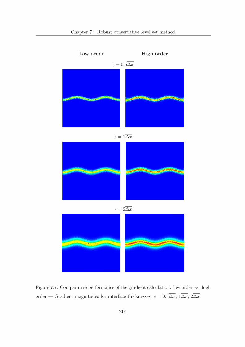
Chapter 7. Robust conservative level set method
Low order High order
ǫ = 0.5∆x
ǫ = 1∆x
ǫ = 2∆x
Figure 7.2: Comparative performance of the gradient calculation: low order vs. high
order — Gradient magnitudes for interface thicknesses: ǫ = 0.5∆x, 1∆x, 2∆x
201

Chapter 7. Robust conservative level set method
Low order High order
ǫ = 0.5∆x
ǫ = 1∆x
ǫ = 2∆x
Figure 7.3: Comparative performance of the gradient calculation: low order vs. high
order — Gradient in the direction x for interface thicknesses: ǫ = 0.5∆x, 1∆x, 2∆x
202
Chapter 7. Robust conservative level set method
7.4 Multidimensional universal limiter with ex-
plicit solution
As noted in [46, 269], WENO schemes are not necessarily total variation bounded
(TVB), even when coupled with a total variation diminishing (TVD) Runge-Kutta
time integration. However, as our conservative level set field represents the liquid
volume fraction in the domain, non-physical values of ϕ such that ϕ < 0 or ϕ > 1
cannot be tolerated. Indeed, such non-physical values may worsen over millions of
time steps and eventually the density, calculated from ϕ, may end up negative in
some cells. This would then crash the solver employed to solve the Navier-Stokes
incompressible equations.
As a result, we decided to use the multidimensional universal limiter with explicit
solution (MULES) of Weller [166], used by default in OpenFOAM to maintain the
boundedness of the VOF field. It is worth mentioning that the addition of such a
flux limiter algorithm to the RCLS will reduce the overall order of accuracy of the
interface-capturing method [3].
To our knowledge, Weller has not presented his algorithm in any publication. The
only available description of the method is given by Masse in [148]. This section
presents the MULES method based on Masse’s thesis and on OpenFOAM’s routine
for MULES.
7.4.1 Overview of the method
MULES calculates a limited flux through the face Fl, FL,l, for the liquid volume
fraction ϕ such that for each cell Ei, the conservative level set at time tn+1, ϕ(n+1)i ,
remains bounded by the minimal and maximal values of the solution in its neigh-
bouring cells Ejl at the previous time step tn :
minjl
(ϕ
(n)jl
)≤ ϕ
(n+1)i ≤ max
jl
(ϕ
(n)jl
)jl = 1, · · · , Li (7.50)
203

Chapter 7. Robust conservative level set method
Let us note ϕ(n+1)i,min and ϕ
(n+1)i,max , respectively the minimum and the maximum ad-
missible values for ϕ(n+1)i in (7.50). To ensure that no non-physical values will be
propagated, both ϕ(n+1)i,min and ϕ
(n+1)i,max are then clipped between 0 and 1, using the
following clipping operator:
clip (x) = max (min (x, 1) , 0) (7.51)
MULES follows the basic principles of the flux-corrected transport (FCT) of Boris
and Book [22–24], in the format described by Zalesak [284]. In order to satisfy the
boundedness criterion (7.50), MULES calculates the limited flux FL,l through Fl
face by face by taking the weighted average of two fluxes for ϕ:
• The flux computed with a first-order upwind scheme for the advection equation
only: FU,l. This flux leads to a bounded solution but is diffusive.
• The sum of the fluxes computed with the high-order scheme (see Chapter 6),
FHO,l, for both the advection equation and the re-initialisation equation. This
flux leads to a high-order accurate solution that is not systematically bounded.
As the weighting varies from face to face, the FCT computation of the limited flux
is non linear.
Introducing the limiter factor λl — calculated for each face Fl of the mesh — the
expression for the limited flux then reads:
FL,l = (1 − λl) FU,l + λlFHO,l (7.52)
The flux of liquid volume fraction Fl through a given face Fl represents the amount
of liquid going through Fl during a given time step ∆t. Although not numerically
calculated as such, the flux is physically identical to:
Fl = |Fl| (Ul · nl)ϕ
where Ul is the face-averaged velocity vector over Fl and nl is the outward face
normal of the cell considered Ei. As a result, the flux is positive when the liquid is
204

Chapter 7. Robust conservative level set method
exiting the cell Ei and negative when entering it. Of course, for two neighbouring
cells Ei and Ej , separated by the face Fl, the flux through Fl is equal in magnitude
and of opposite sign for each cell.
Introducing the correction flux FC,l defined as the difference between FHO,l and
FU,l:
FC,l = FHO,l − FU,l (7.53)
The expression for the limited flux (7.52) can then be re-written as:
FL,l = FU,l + λlFC,l (7.54)
Once the limiter factor computed and the limited flux calculated according to
(7.54), the scalar field ϕ is updated using an Euler time integration, such that:
ϕ(n+1)i = ϕ
(n)i − ∆t
|Ei|
Li∑
l=1
FL,l (7.55)
7.4.2 Determination of the limiter factor
The limiter factor λl is calculated iteratively such that the boundedness condition
(7.50) is satisfied. λl directly derives from the re-formulation of the condition (7.50)
in terms of fluxes. The bounds for the liquid volume fraction in Ei at time tn+1
correspond, in terms of fluxes, to the maximum temporal variation of liquid volume
in Ei,(
∆Vliq
∆t
)
i:
• The minimum ϕ(n+1)i,min corresponds to the maximum decrease of liquid volume
in Ei.
• The maximum ϕ(n+1)i,max corresponds to the maximum increase of liquid volume
in Ei.
205
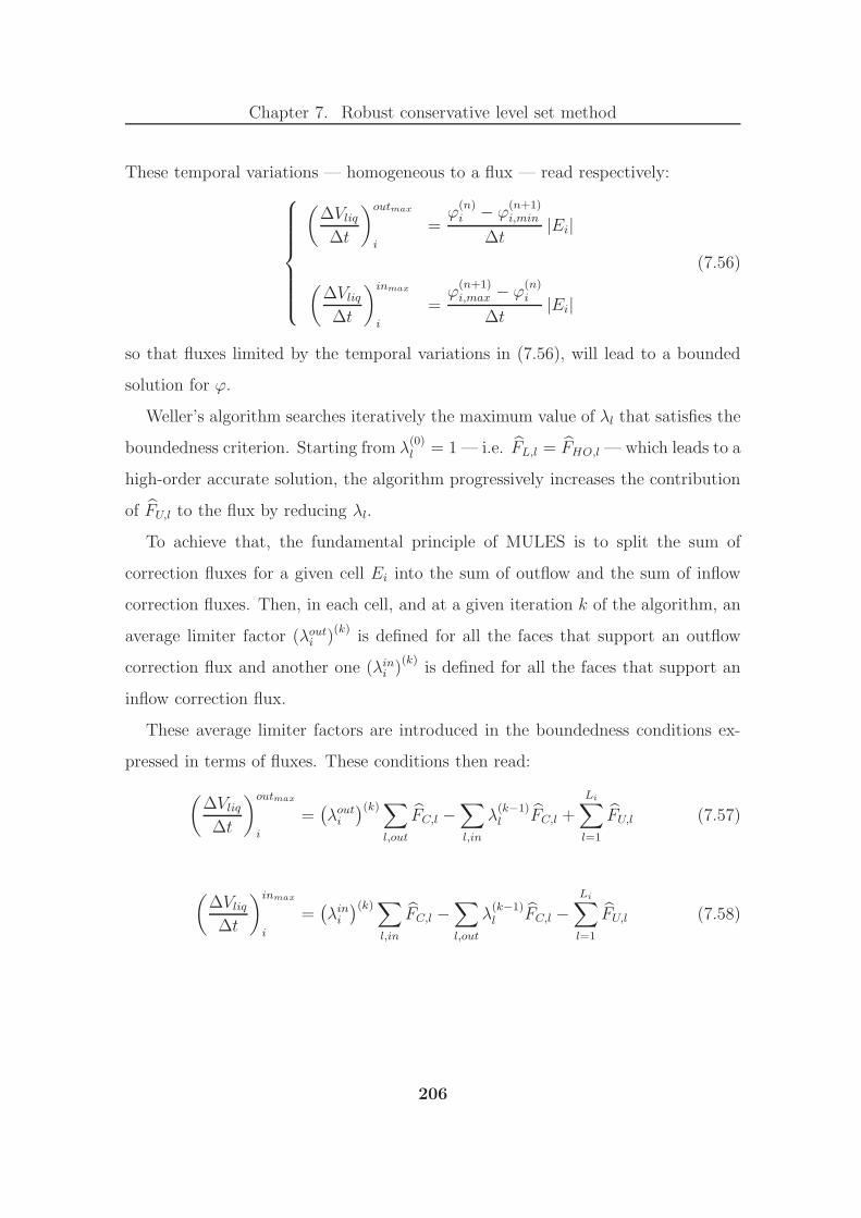
Chapter 7. Robust conservative level set method
These temporal variations — homogeneous to a flux — read respectively:
(∆Vliq∆t
)outmax
i
=ϕ
(n)i − ϕ
(n+1)i,min
∆t|Ei|
(∆Vliq∆t
)inmax
i
=ϕ
(n+1)i,max − ϕ
(n)i
∆t|Ei|
(7.56)
so that fluxes limited by the temporal variations in (7.56), will lead to a bounded
solution for ϕ.
Weller’s algorithm searches iteratively the maximum value of λl that satisfies the
boundedness criterion. Starting from λ(0)l = 1 — i.e. FL,l = FHO,l — which leads to a
high-order accurate solution, the algorithm progressively increases the contribution
of FU,l to the flux by reducing λl.
To achieve that, the fundamental principle of MULES is to split the sum of
correction fluxes for a given cell Ei into the sum of outflow and the sum of inflow
correction fluxes. Then, in each cell, and at a given iteration k of the algorithm, an
average limiter factor (λouti )(k)
is defined for all the faces that support an outflow
correction flux and another one (λini )(k)
is defined for all the faces that support an
inflow correction flux.
These average limiter factors are introduced in the boundedness conditions ex-
pressed in terms of fluxes. These conditions then read:
(∆Vliq∆t
)outmax
i
=(λouti
)(k)∑
l,out
FC,l −∑
l,in
λ(k−1)l FC,l +
Li∑
l=1
FU,l (7.57)
(∆Vliq∆t
)inmax
i
=(λini)(k)∑
l,in
FC,l −∑
l,out
λ(k−1)l FC,l −
Li∑
l=1
FU,l (7.58)
206
Chapter 7. Robust conservative level set method
where the sums of outflow and inflow fluxes in Ei are calculated the following way
for a given flux Fl:
∑
l,out
Fl =
Li∑
l=1
max(Fl, 0
)
∑
l,in
Fl =
Li∑
l=1
min(Fl, 0
)(7.59)
As a flux exiting a cell — and therefore decreasing the amount of liquid volume
in the cell — is positive, the sum of upwind fluxes FU,l on all the faces of Ei is then
added on the r.h.s. of (7.57). Similarly, the sum of upwind fluxes is subtracted on
the r.h.s. of (7.58).
The average limiter factors (λouti )(k)
and (λini )(k)
are then calculated from (7.57)
and (7.58) respectively.
As can be seen in the boundedness condition relating to the maximum decrease in
liquid volume (7.57), (λouti )(k)
weights the sum of outflow correction fluxes while the
limiter factor obtained at the previous iteration λ(k−1)l weights individually each of
the corresponding inflow correction fluxes. Similarly, in the boundedness condition
relating to the maximum increase in liquid volume (7.58), (λini )(k)
weights the sum
of inflow correction fluxes while the limiter factor obtained at the previous iteration
λ(k−1)l weights individually each of the corresponding outflow correction fluxes.
Then, the algorithm takes as limiter factor for the face Fl at the current iteration
k, λ(k)l , the minimum of three values:
• The relevant average limiter factor in one of the adjacent cells Ei: (λouti )(k)
if
the correction flux through Fl is exiting Ei, (λini )(k)
otherwise.
• The relevant average limiter factor in the other adjacent cell Ej :(λinj)(k)
if the
correction flux through Fl is entering Ej ,(λoutj
)(k)otherwise.
• The limiter factor at the previous iteration: λ(k−1)l .
207

Chapter 7. Robust conservative level set method
The algorithm iterates m times — with m specified by the user — to produce a
final limiter factor λ(m)l for each face Fl of the mesh.
7.5 Performance of the method
This section compares the performance of the RCLS with established multiphase
numerical methods:
• The VOF method of OpenFOAM: interFoam
• The accurate conservative level set (ACLS) method of Desjardins et al. [46, 47]
For this comparative study, the RCLS transports the scalar field ϕ using a
WENO3 scheme, the CLS coefficient is set to ǫ = 0.5∆x and the re-initialisation
of the hyperbolic tangent profile is only performed every five time steps (see Sec-
tion 9.2.2).
Comparison with interFoam
The relative performance of the transport algorithms is assessed on the following
test cases (defined in Section 4.2.1): Zalesak’s slotted disk (on a 1282 Cartesian
mesh) and the disk in a deformation field (on a 2562 Cartesian mesh).
As can be seen in Figure 7.4, the RCLS method clearly outperforms interFoam
on both test cases. In particular, the ligament predicted by our transport algorithm
is longer and the interface is free from non-physical wiggles.
Comparison with ACLS
In order to compare the method of Desjardins et al. with the RCLS, we have
performed the computation of the disk in a deformation field as set in [47]. In this
publication, the deformation field defined by the authors differs from the one given
208
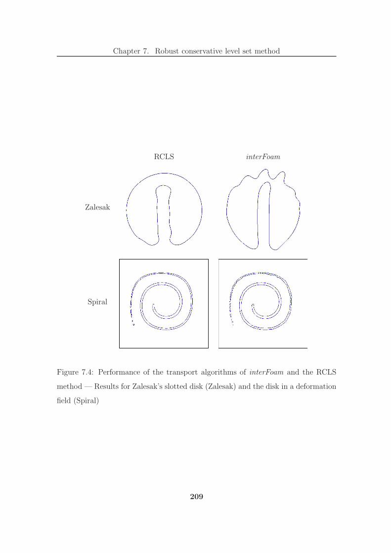
Chapter 7. Robust conservative level set method
RCLS interFoam
Zalesak
Spiral
Figure 7.4: Performance of the transport algorithms of interFoam and the RCLS
method — Results for Zalesak’s slotted disk (Zalesak) and the disk in a deformation
field (Spiral)
209
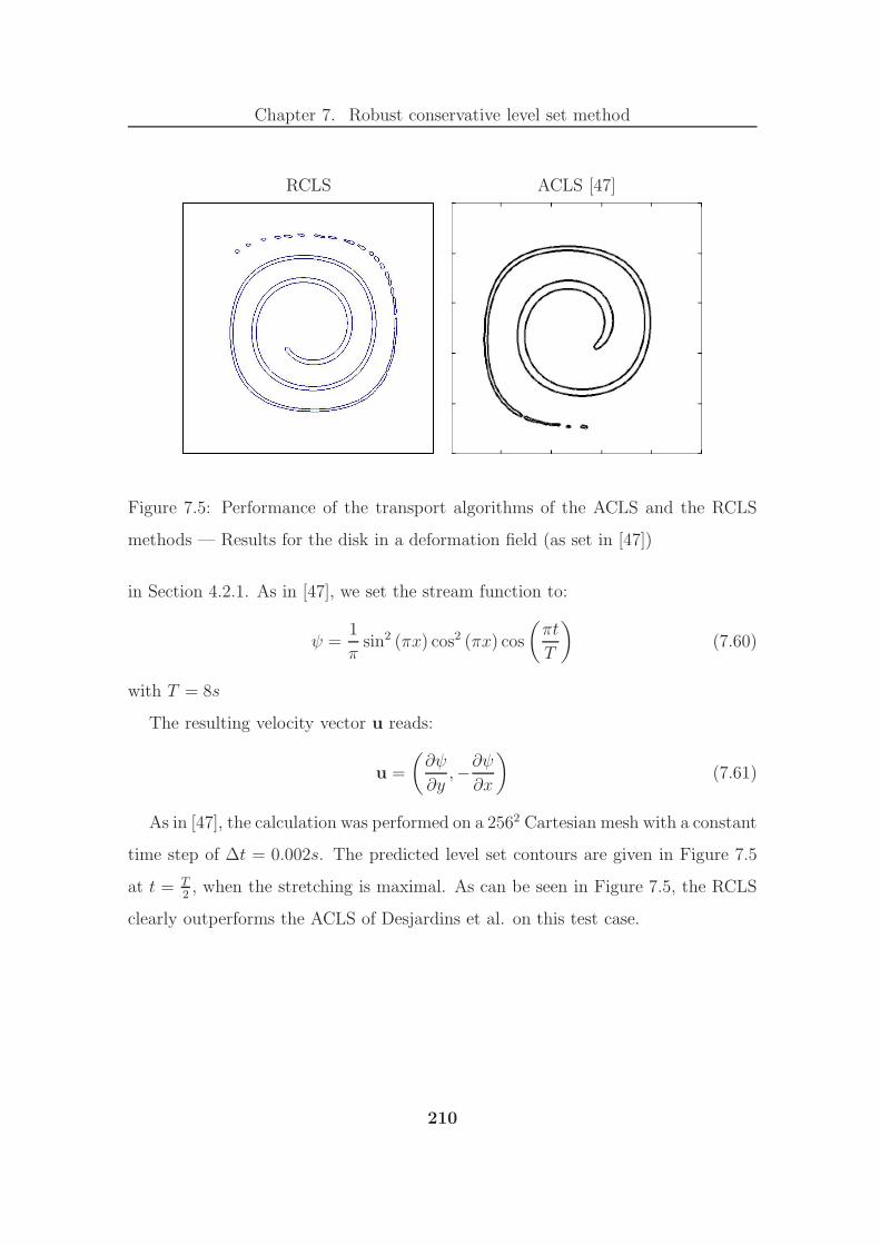
Chapter 7. Robust conservative level set method
RCLS ACLS [47]
Figure 7.5: Performance of the transport algorithms of the ACLS and the RCLS
methods — Results for the disk in a deformation field (as set in [47])
in Section 4.2.1. As in [47], we set the stream function to:
ψ =1
πsin2 (πx) cos2 (πx) cos
(πt
T
)(7.60)
with T = 8s
The resulting velocity vector u reads:
u =
(∂ψ
∂y,−∂ψ
∂x
)(7.61)
As in [47], the calculation was performed on a 2562 Cartesian mesh with a constant
time step of ∆t = 0.002s. The predicted level set contours are given in Figure 7.5
at t = T2, when the stretching is maximal. As can be seen in Figure 7.5, the RCLS
clearly outperforms the ACLS of Desjardins et al. on this test case.
210

Chapter 7. Robust conservative level set method
7.6 Interpretation of the method
The RCLS method transports a scalar ϕ defined as the hyperbolic tangent profile
of the signed distance to the interface. The scalar ϕ is transported in a conservative
manner (see Chapter 6) such that it remains conserved to machine accuracy (Lax
and Wendroff provided some theoretical background for this assertion in [121] and
our numerical experiments, presented in Section 8.4, confirm it). In addition, the
transition between phases, characterised by this hyperbolic tangent profile, is kept
to a constant thickness.
If applied in the same spirit as Olsson and Kreiss [163] and Desjardins et al. [47],
the RCLS method transports a function of the distance to the interface. The phase
boundary being defined by the contour ϕ = 0.5, all the volume encompassed by that
surface can be considered as filled with liquid. Such an interpretation of ϕ leads to
a level set formulation of the RCLS.
However, as the interface thickness is kept constant, the scalar transported ϕ can
be identified to the liquid volume fraction (see Section 7.1). When interpreting ϕ
as such, the RCLS resembles a VOF method with an interface of constant thick-
ness. The interface reconstruction generally required by VOF methods is no longer
required here, as the hyperbolic tangent profile provides a smooth field to calculate
the interface gradient.
The RCLS method can therefore be perceived as both a level set method and a
volume of fluid method.
211

Chapter 8
A mass-conservative method for
efficient atomisation modelling in
parallel
At run time, the modelling capability developed involves three main building blocks:
the transport of the level set scalar ϕ, the pressure-velocity coupling and the output
of droplet boundary conditions for Lagrangian spray models. All of these operations
are performed in a conservative way such that throughout the whole computation
no mass is lost.
The transport of the level set is the main item of this work and has already been
described in chapters 6 and 7. In this chapter we present the additional building
blocks that make the code readily applicable to the atomisation of liquid sheets. In
particular, the solution of the incompressible Navier-Stokes equations is detailed in
Section 8.1, the algorithm for the droplet transfer is explained in Section 8.2 and
the parallelisation of the whole code is reviewed in Section 8.3. Finally, the perfor-
mance of the modelling capability on typical two-phase flow test cases is reported
in Section 8.4.
212
Chapter 8. A mass-conservative method for efficient atomisation modelling inparallel
8.1 Solution of the incompressible Navier-Stokes
equations
8.1.1 Conservative formulation
The governing equations for multiphase flows with interface modelling are given
in Chapter 3. Implementing in these equations the CSF description of the sur-
face tension (see Chapter 3), leads to the following conservation formulation of the
incompressible Navier-Stokes equations:
∇ · u = 0 (8.1)
∂ (ρu)
∂t+ ∇ · (ρu ⊗ u) = −∇p + ρg + σκ∇ϕ+ ∇ · (2µD) (8.2)
where the rate-of-strain tensor D reads:
D =1
2
(∇u + (∇u)T
)(8.3)
In his implementation of the incompressible Navier-Stokes equations, Weller re-
formulates some terms of the momentum equation (8.2). In particular, the viscous
stress term is re-expressed to improve the efficiency of its numerical determination
[208]:
∇ · (2µD) = ∇ ·(µ(∇u + (∇u)T
))
= ∇ · (µ∇u) + (∇u) · ∇µ+ µ∇ (∇ · u)
= ∇ · (µ∇u) + (∇u) · ∇µ (8.4)
Similarly, a modified pressure pd is introduced to simplify the specification of the
pressure boundary conditions [208]. pd is defined by:
pd = p− ρg · x (8.5)
The gradient of pd then reads:
∇pd = ∇p− ρg − (g · x)∇ρ (8.6)
213

Chapter 8. A mass-conservative method for efficient atomisation modelling inparallel
Finally, inserting (8.4) and (8.6) into (8.2) leads to the formulation of the momentum
equation as used in the code:
∂ (ρu)
∂t+∇· (ρu⊗ u) = −∇pd +∇· (µ∇u)+ (∇u) ·∇µ− (g · x)∇ρ+σκ∇ϕ (8.7)
Before describing the solution procedure for the system of equations formed by
(8.1) and (8.7), let us consider the system of linear algebraic equations resulting
from the discretisation of these governing equations.
8.1.2 Systems of linear algebraic equations
Although the methodology presented in this sub-section applies directly to any ten-
sorial quantity, for the sake of clarity we will consider a vector variable u. For each
control volume Ei of a mesh that contains N cells, the discretisation procedure of
the governing equation for u leads to the following algebraic equation at the time
tn:
aiuni +
∑
j
ajunj = ri (8.8)
where ui and uj refer to the value of u in, respectively, the considered element Ei
and its neighbours Ej . The coefficients ai, aj and the vector ri result from the
discretisation of the governing equation for u.
As the solution in the considered cell ui depends on the solution in its neighbour-
ing cells uj , writing the equation (8.8) for each control volume produces a systems
of algebraic equations. This system can be expressed in the following matrix form:
AU = R (8.9)
where:
A is a N × N matrix of scalars. This square matrix is sparse and is made of
the ai coefficients on the diagonal and of the aj coefficients elsewhere.
214

Chapter 8. A mass-conservative method for efficient atomisation modelling inparallel
U is a vector of vectors. This column vector gathers N vectors, one for each
cell in the mesh. In particular, the ith row of the vector U contains ui: the
solution in the cell Ei.
R is a vector of vectors. This column vector gathers N vectors, one for each
cell in the mesh. Similarly to U, the ith row of the vector R contains ri: the
source vector for the cell Ei.
The matrix A can be split into two matrices: a diagonal matrix AD that gathers
the coefficients ai and the matrix AOD which contains the off-diagonal coefficients
aj :
A = AD + AOD (8.10)
AD being diagonal, it only contains N scalar elements that can be stored in the
column vector AD.
Let us now introduce the vector of vectors AH, defined by:
AH = R −AODU (8.11)
The next sub-section, which describes the handling of the pressure-velocity cou-
pling, involves semi-implicit discretisations of the equations (8.1) and (8.7). In that
solution procedure, the data contained in AD and AH is used in conjunction with
terms of the momentum equation treated explicitly. In these data manipulations,
AD and AH should no longer be perceived as vectors but as fields: AD correspond-
ing to a scalar field and AH to a vector field. In order to remain coherent in terms
of notation, we note the scalar field relating to AD: aD and the vector field relating
to AH : aH .
8.1.3 Pressure-velocity coupling
The incompressible Navier-Stokes equations are discretised in a semi-implicit man-
ner such that the restriction on the time step remains low. The pressure veloc-
ity coupling is handled with the pressure-implicit with splitting operators (PISO)
215

Chapter 8. A mass-conservative method for efficient atomisation modelling inparallel
method of Issa [99]. This non-iterative method proceeds through a series of predic-
tor and corrector steps that approximate the exact velocity and pressure fields with
improving accuracy as the number of PISO loops increases.
The method as implemented in the code involve three steps: the “momentum
predictor”, the “pressure solution” and the “explicit velocity correction” [103]. The
last two steps being iterated as many times as required to reach a given accuracy.
Issa demonstrates that two loops are sufficient if the equations are discretised with
second-order accurate schemes [99].
In his implementation of the PISO algorithm, Weller uses the principle of the
pseudo-staggered grid of the Rhie and Chow interpolation [199] to remove the
checker-board pressure oscillation. In that procedure, Weller introduces the vol-
umetric flow rate Q stored at the face centres. The scalar Ql associated to the face
Fl corresponds to:
Ql = ul · Fl (8.12)
where Fl = |Fl|nlHowever, Ql is not calculated directly from (8.12) because the velocity field u
being a collocated variable, ul would have to be interpolated and the field Q would
not satisfy the continuity equation.
It is convenient to use the volumetric flow rate as a variable in a finite volume
framework for incompressible flows because this quantity often appears in the dis-
cretised formulations of the equations through the application of Gauss’ theorem.
Momentum predictor
In order to calculate the predicted velocity Weller applies the following semi-implicit
discretisation to (8.7):
[[∂ρ [u]
∂t
]]+J∇·(ρu ⊗ [u])K = −∇pd+J∇·(µ∇ [u])K+(∇u) ·∇µ−(g · x)∇ρ+σκ∇ϕ
(8.13)
216
Chapter 8. A mass-conservative method for efficient atomisation modelling inparallel
In (8.13), we are using same convention as Weller’s [208, 272], which notes in
double brackets the terms treated implicitly and in single brackets the sought vari-
able of the equation. Therefore in (8.13), while the unsteady term, the convection
term and the diffusion term are treated implicitly, all the other terms are treated
explicitly. Besides, only the velocity vectors in single brackets, [u], are unknown.
As all other quantities are taken from the previous time step, the notation implies
that the convection term is linearised.
Let us detail how the convection and the diffusion terms are discretised:
• The volume integration and the linearisation of the convection term are applied
the following way:
∫∫∫
Ei
∇ · (ρu ⊗ [u]) dEi =
Li∑
l=1
Fl · (ρu ⊗ [u])l
=
Li∑
l=1
(Fl · ul) (ρ [u])l
=
Li∑
l=1
Ql (ρ [u])l (8.14)
in which Ql, taken from the previous time step, satisfies the continuity equa-
tion.
• The volume integration of the diffusion term leads to:
∫∫∫
Ei
∇ · (µ∇ [u]) dEi =
Li∑
l=1
Fl · (µ∇ [u])l
=
Li∑
l=1
µlFl · (∇ [u])l (8.15)
NB: All throughout this section, the subscript l refers to the face value of the
associated quantity.
The solution of the discretised equation (8.13) produces a first guess for the
velocity: u∗ (as noted by Issa in [99]) which does not satisfy the continuity equation.
217
Chapter 8. A mass-conservative method for efficient atomisation modelling inparallel
Pressure solution
Let us write below the momentum equation without the surface tension force, the
gravity force and the pressure gradient:
∂ (ρu)
∂t+ ∇ · (ρu ⊗ u) = ∇ · (µ∇u) + (∇u) · ∇µ (8.16)
The equation (8.16) is discretised in the same semi-implicit way as was the equa-
tion (8.7) in the momentum predictor step:
[[∂ρ [u]
∂t
]]+ J∇ · (ρu ⊗ [u])K = J∇ · (µ∇ [u])K + (∇u) · ∇µ (8.17)
As described in Section 8.1.2, a semi-implicitly discretised equation such as (8.17)
results in a system of algebraic equations that can be put in a matrix form. We note
A, the matrix of that algebraic system.
Two fields are then constructed from the system of algebraic equations resulting
from (8.17) (see Section 8.1.2):
• A scalar field aD gathering the diagonal coefficients of A.
• A vector field aH built from the off-diagonal coefficients of A, the source vector
and the predicted velocity field u∗.
Introducing aD and aH in (8.13), leads to the following semi-discretised formula-
tion of the momentum equation:
u =1
aD(aH − (g · x)∇ρ+ σκ∇ϕ) − 1
aD∇pd (8.18)
The first term on the right hand side of (8.18) is homogeneous to a velocity, but
lacks the contribution of the pressure gradient to satisfy the momentum equation.
We denote it as uNP and rewrite (8.18) as:
u = uNP − 1
aD∇pd (8.19)
218
Chapter 8. A mass-conservative method for efficient atomisation modelling inparallel
Expressing the velocities on the cell face ul as the face interpolation of (8.19) leads
to:
ul = uNPl −(
1
aD
)
l
(∇pd)l (8.20)
As u is now sought such that it satisfies the continuity equation, introducing (8.19)
in (8.1) leads to:
∇ · uNP = ∇ ·(
1
aD∇pd
)(8.21)
Calculating the volume integration of (8.21) using Gauss’ theorem results in:
Li∑
l=1
Fl · uNPl =
Li∑
l=1
Fl ·((
1
aD
)
l
(∇pd)l)
(8.22)
Li∑
l=1
QNPl =
Li∑
l=1
Fl ·((
1
aD
)
l
(∇pd)l)
(8.23)
where QNPl is the volumetric flow rate associated to uNPl . Weller calculates QNP
l
according to:
QNPl =
(1
aD
)
l
(Fl · (aH)l − (g · x)l Fl · (∇ρ)l + (σκ)l (∇ϕ)l
)(8.24)
The solution of (8.23) provides the new pressure field noted p∗d by Issa in [99].
Explicit velocity correction
The volumetric flow rates are then updated according to:
Ql = Fl · ul
= Fl ·(uNPl −
(1
aD
)
l
(∇pd)l)
= QNPl − Fl ·
((1
aD
)
l
(∇pd)l)
(8.25)
As (8.22) is satisfied, the updated volumetric flow rates are conservative.
219
Chapter 8. A mass-conservative method for efficient atomisation modelling inparallel
Weller then reconstructs the velocity field from Q starting with the following
assumption:Li∑
l=1
nl (Fl · u) =
Li∑
l=1
nl (Fl · ul) (8.26)
Now, let us introduce the symmetric tensor Dl = nl ⊗ Sl. The dyad Dl has the
following property:
Dl · u = (nl ⊗ Fl) · u
= nl (Fl · u) (8.27)
where Dl maps the velocity vector u onto a vector parallel to nl with a magnitude
|nl| (Fl · u) ≈ Ql. Therefore Dl maps u onto a vector ≈ nlQl.
Introducing (8.27) into (8.26), leads to:
Li∑
l=1
((nl ⊗ Fl︸ ︷︷ ︸
Dl
) · u)
=
Li∑
l=1
nl (Fl · ul) (8.28)
Applying to the left hand side of (8.28) the distributivity of the inner product of a
tensor by a vector, and replacing Fl · ul by the volumetric flow rate Ql on the right
hand side of (8.28) leads to:
(Li∑
l=1
Dl
)· u =
Li∑
l=1
nlQl (8.29)
Let us now introduce the symmetric tensor D defined by:
D =
Li∑
l=1
Dl (8.30)
Since D is symmetric and made of real coefficients, it can be inverted. Multiplying
on either side of (8.29) by D−1 finally provides the reconstructed velocity field:
u = D−1 ·(
Li∑
l=1
nlQl
)
=
(Li∑
l=1
nl ⊗ Fl
)−1
·(
Li∑
l=1
nlQl
)(8.31)
220
Chapter 8. A mass-conservative method for efficient atomisation modelling inparallel
The velocity field produced by equation (8.31) is the new velocity field denoted as
u∗∗ by Issa in [99]. The solution procedure then repeats the pressure solution and
the explicit velocity correction steps a given number of times. Each new iteration of
the PISO loop starts from the pressure and velocity fields calculated at the previous
PISO iteration.
Typically, the systems of algebraic equations produced for the pressure-velocity
coupling are solved by using either the pre-conditioned conjugate gradient (PCG)
or the generalised geometric-algebraic multi-grid (GAMG).
8.2 Droplet transfer
8.2.1 Motivations
The need for droplet transfer arises from the computational modelling of atomisa-
tion. As described in Chapter 2, the process of atomisation transforms a jet of liquid
into droplets. It generally involves two stages: the primary breakup where drops
are detaching from the core of the liquid jet and the secondary breakup where the
droplets produced at the previous stage further disintegrate into smaller droplets.
Although there are some reliable secondary breakup models, the primary breakup
— highly dependent on the geometry of the injection device — has to be modelled
directly using interface description methods like RCLS. However, the faithful mod-
elling of the spray requires the simulation of both the primary and the secondary
breakups. In order to reduce the computational cost of the modelling capability
Kim et al. [111] had the idea to remove the droplets from the level set formulation
to send them into a Lagrange tracking framework equipped with an appropriate
secondary breakup model.
This strategy allows the modelling capability to represent both types of breakup in
the same computation while significantly reducing the computational cost. Indeed,
as illustrated in Section 4.3, under aero-engine conditions, the droplet size can reduce
221
Chapter 8. A mass-conservative method for efficient atomisation modelling inparallel
to very small values and the mesh refinement required to resolve such small liquid
structures is unaffordable.
8.2.2 Outline of the method
In our implementation, the droplets satisfying certain criteria (see Section 8.2.4)
are removed from the level set field ϕ at specific times tnR. In order to reduce the
computational cost, this transfer only occurs at the output time step (time step
at which the fields computed are written out by the code). This strategy aims
at providing a better trade-off in terms of computational cost versus resolution of
droplets.
Once identified and removed from the field ϕ, the droplets are then stored in two
ways:
• The level set field associated with the removed droplets is stored into a “Drops”
field. Therefore, “Drops” is the level set field gathering all the drops produced
between tn−1R and tnR in the state in which they were at tnR. The field “Drops”
has two purposes: it allows us to conduct further analysis on the droplets
(calculation of specific geometrical parameters, etc. . . ) and gives the option
to restart from tnR with the level set field as it was before the droplet removal.
• Some characteristics of the droplets removed at tnR are calculated and stored
in lists (Section 8.2.5). These data are the boundary conditions required by
Lagrange tracking schemes to simulate the spray with a secondary breakup
model. Once produced on a sub-model of a fuel injector, these lists can be
imported by combustion codes for the simulation of the reacting flow in a
combustion chamber.
The algorithm operates the transfer of droplets in five steps:
1. Blob search: this routine searches through the computational domain to iden-
tify coherent liquid structures of any shape and size.
222
Chapter 8. A mass-conservative method for efficient atomisation modelling inparallel
2. Drop selection: the algorithm searches through the blobs identified and se-
lects the ones that match the droplet criteria (see Section 8.2.4). Because
the selection criteria are based on droplet characteristics, the generation of
the boundary conditions for the Lagrange tracking schemes is also performed
during this step.
3. Transfer drops: the level set field associated to the droplets is removed from
the field ϕ. After this step, the hyperbolic tangent profile is lost.
4. Write drop characteristics: the boundary conditions for the combustion codes
are written out.
5. Re-initialisation of ϕ: the level set field is re-initialised in order to reconstruct
the hyperbolic tangent profile of ϕ. As the re-initialisation is done in a con-
servative way, this step does not affect the mass conservation properties of the
modelling capability.
8.2.3 Identification of blobs
Definition of a blob
We consider blobs as liquid structures of arbitrary shapes, sizes, positions and ve-
locities. The search algorithm defines a blob B as a group of cells Ei that satisfies
the following criteria (see Figure 8.1 for a 1D representation of the criteria given
below):
• The cells Ei are face-neighbours, i.e. each cell of the blob shares at least one
face with another cell of the blob (see Figure 8.3 for an illustration on a 2D
mesh.).
• In each cell of the blob, the liquid volume fraction is above a given threshold
ϕLmin, such that it can be considered as containing some liquid. This condition
223

Chapter 8. A mass-conservative method for efficient atomisation modelling inparallel
reads:
∀Ei ∈ B : ϕi ≥ ϕLmin (8.32)
• All the cells Ek surrounding the blob B — i.e. sharing at least one face with a
cell Ei of B — have a liquid volume fraction below ϕLmin, such that they can
be considered as “gas”. This condition reads:
∀Ek ∈ face-neighbours ofEi : ϕk < ϕLmin (8.33)
Search algorithm
The search algorithm starts by storing all the cells containing liquid into the list
“liqRest”. Then, as long as the list “liqRest” is not empty, the routine performs the
following operations:
1. Consider the first element of “liqRest”: E1
2. Add layers of cells around E1 in a similar way that cells were gathered for the
generation of a central stencil in Chapter 6 (see Section 6.3.1). However, here
the layers consist of face-neighbours of the cells belonging to the previous layer,
that are not already in the blob and that contain some liquid (see condition
(8.32)). The addition of layers is continued until the algorithm produces an
empty list for the current layer. At that point, no face-neighbour with a liquid
volume fraction greater or equal to ϕLmin could be found by the algorithm,
such that the blob is surrounded by “gas”.
3. Remove the cells of the blob constituted from the list “liqRest”. As a result,
that list only gathers cells that contain liquid and that have not yet been
attributed to a blob.
224

Chapter 8. A mass-conservative method for efficient atomisation modelling inparallel
Figure 8.1: Schematic of a blob on a 1D mesh — Hyperbolic tangent profile (in red),
liquid volume fraction in the blob (light green) and liquid volume fraction outside
of the blob (in purple)
8.2.4 Selection of drops
Definition of a droplet
Once the list of blobs constructed from the level set field ϕ, the selection algorithm
identifies the liquid structures that qualify as droplets. We choose to define a droplet
D as a group of ND cells Ei that satisfies the following criteria:
• A droplet contains at least one cell with a volume fraction above a given
threshold: ϕDmin.
• A droplet has an equivalent diameter Deq smaller than a given threshold:
Dmax.
• A droplet has to be fairly spherical.
• As it is about to be sent into a Lagrange tracking scheme, a droplet should not
be on the verge of coalescing with the core of the liquid jet C (largest liquid
structure).
225

Chapter 8. A mass-conservative method for efficient atomisation modelling inparallel
Figure 8.2: Illustration of the principle of face-neighbours used to define blobs
The first criterion can be expressed the following way:
∃Ej ∈ D | ϕj ≥ ϕDmin (8.34)
As mentioned in Section 7.2, the solution of the advection equation diffuses the
hyperbolic tangent profile, such that patches of cells containing small amounts of
liquid may appear in the solution. Although the re-initialisation of the profile will
get rid of these patches, the user has the option to solve the re-initialisation equation
only periodically and not at every time step (see Section 9.2.2). In the case of a
droplet transfer occurring between two re-initialisation steps, the criterion (8.34)
guarantees that these patches are not mistaken for droplets.
The limitation on the droplet size (second criterion) reads:
Deq ≤ Dmax (8.35)
Introducing the volume of the droplet VD, the equivalent diameter reads:
Deq =3
√6VDπ
(8.36)
This maximum diameter can be set by the user either as a multiple of ∆x (char-
acteristic length scale of the mesh) or as an actual dimension in metres. In order
to simulate directly the secondary breakup or to account for the coalescence of the
blobs, the user may want to keep in the level set formulation all the liquid structures
226

Chapter 8. A mass-conservative method for efficient atomisation modelling inparallel
that can be resolved by the mesh. However, depending on the parameters of the La-
grangian spray model and on the targeted computational cost, it may be necessary
to increase Dmax.
After Kim et al. [111], we choose the following expression for the sphericity
criterion:
rmax < Deq (8.37)
The condition (8.37) formulates that the maximum radius of the droplet rmax is
smaller than the droplet’s equivalent diameter. We define rmax as the maximum
distance between the centre of mass of the droplet CD and the centre of a cell
belonging to the droplet Ci. The expression for rmax reads:
rmax = maxEi∈D
(∣∣∣−−−→CDCi
∣∣∣)
(8.38)
This criterion ensures that non-spherical blobs — such as detached ligaments —
remain in the level set field. Typically, detached ligaments would undergo Plateau-
Rayleigh instabilities and breakup into a row of droplets. Such breakup phenomena
are not generally accounted for by Lagrangian spray models.
Berlemont has observed small broken-off droplets flowing back into the core of
the liquid jet in DNS studies of round jet atomisation [1]. To account for this
phenomenon we have introduced a direction criterion in the droplet selection (see
Figure 8.3 for an illustration in 2D). Introducing the droplet and liquid core centres
of mass, respectively CD and CC, and the relative droplet velocity (with respect to
the liquid core):−→∆u = uD−uC , we express the direction criterion the following way:
−→∆u · −−−→CCCD > 0 (8.39)
In order to account for both the droplets flowing towards the liquid core and the
droplets being caught up by the liquid jet, the criterion involves the dot product of
the relative droplet velocity with the relative droplet position (with respect to the
centre of mass of the liquid core). Although this criterion does not guarantee to
227

Chapter 8. A mass-conservative method for efficient atomisation modelling inparallel
leave in the level set field all the droplets that would coalesce with the liquid core,
it is calculated quickly and remains quite effective.
Figure 8.3: Illustration of the direction criterion for the droplet selection — For the
pictured velocities and positions of the droplet D and the liquid core C, the direction
criterion is not met and D is left in the level set field
Selection algorithm
The selection algorithm progresses through the list of blobs and assesses whether
the current blob qualifies as a droplet. To improve the efficiency of the selection
process, the routine evaluates the droplet criteria in sequence, performing the most
discriminating tests first. As soon as a test is failed, the code skips to the next blob
in the list.
First, the routine identifies the core of the liquid jet and computes its properties
for the determination of the direction criterion. The liquid core is defined as the
largest blob that contains at least NC cells. The minimum number of cells in the
liquid core NC is either set directly by the user or through the specification of the
characteristic length scale of the liquid jet.
Then, the code goes through the list of blobs produced by the search algorithm
and performs the following steps:
1. Test whether the current blob B contains more than NC elements. If so go to
the next blob.
2. Check that the blob contains at least one cell Ej with ϕj ≥ ϕDmin. If it does
not go to the next blob.
228

Chapter 8. A mass-conservative method for efficient atomisation modelling inparallel
3. Calculate the characteristics of the blobs: volume VB, centre of mass CB, mass-
averaged velocity uB, mass mB and momentum pB. As the calculation of these
quantities involves going through all the cells in the current blob, they are all
performed in the same step.
4. Calculate the equivalent diameter of the blob: DeqB from VB using (8.36). Test
if DeqB is larger than the maximum diameter Dmax. If so, go to the next blob.
5. Calculate the maximum radius of the liquid structure from the blob’s centre
of mass CB by applying (8.38). Test the sphericity of the current blob. If it
does not satisfy the condition (8.37), go to the next blob.
6. If the domain contains cyclic or processor boundary conditions BCcyclic (see
Section 8.3), test if the current blob contains a cell on the border BCcyclic. If
so, go to the next blob.
7. Test the direction criterion for the current blob. If it does not satisfy (8.39),
go to the next blob.
8. At this point of the loop, the current blob has satisfied all the droplet criteria.
Therefore its characteristics, calculated in the previous steps, are stored in the
relevant droplet lists.
8.2.5 Drop characteristics of interest
Droplet removal techniques
As mentioned in Section 7.1, the conservative level set method transports a hyper-
bolic tangent profile ϕ of the signed distance function from the interface φ. As a
result, the level set field ϕ only tends to zero or one, at an infinite distance in,
respectively, the gas phase or the liquid phase. We handle this ambiguity in the
definition of blobs (Section 8.2.3) by considering that a cell Ei contains some liquid
229

Chapter 8. A mass-conservative method for efficient atomisation modelling inparallel
if the associated level set scalar ϕi is above a minimum threshold ϕLmin. It results,
that several options are available to remove the droplets from the level set field.
Figure 8.4: Illustration of the first droplet removal technique: “option 1”
The code offers to the user two means of removing the droplets. The first option
(“option 1”) is to remove all of the “liquid volume fraction” by setting ϕi = 0 in all
the cells Ei that belong to the considered droplet D. The other option (“option 2”)
is to truncate the profile by removing only ϕi − ϕLmin from each droplet cell, thus
setting ϕi = ϕLmin in each cell of D. Figures 8.4 and 8.5 present the fields obtained
after removing the blob pictured in Figure 8.1 using respectively the first and the
second technique. After the droplet removal the level set field is re-initialised (in a
conservative manner), such that the hyperbolic tangent profile is recovered.
Depending on the technique chosen, the droplet characteristics are not calculated
in the same way. Indeed, it is crucial to account for liquid volume fraction actually
removed in order to maintain mass conservation all the way through the calculation.
Characteristics outputted
Some droplet characteristics are calculated from the amount of liquid in each cell of
the droplet. As a result, depending on the option chosen by the user, two alternative
230

Chapter 8. A mass-conservative method for efficient atomisation modelling inparallel
Figure 8.5: Illustration of the second droplet removal technique: “option 2”
formulae exist to compute these quantities.
The droplets characteristics calculated and stored by the algorithm are:
• The volume VD, given by:
Option 1: VD =
ND∑
i=1
|Ei|ϕi (8.40)
Option 2: VD =
ND∑
i=1
|Ei| (ϕi − ϕLmin) (8.41)
• The mass mD, calculated from VD according to:
mD = ρliqVD (8.42)
• The centre of mass CD, expressed as:
Option 1:−−→OCD =
1
VD
ND∑
i=1
|Ei|ϕi−−→OCi (8.43)
Option 2:−−→OCD =
1
VD
ND∑
i=1
|Ei| (ϕi − ϕLmin)−−→OCi (8.44)
231

Chapter 8. A mass-conservative method for efficient atomisation modelling inparallel
• The mass-averaged velocity vector uD, given by (8.45) and (8.46) below:
Option 1: uD =1
VD
ND∑
i=1
|Ei|ϕiui (8.45)
Option 2: uD =1
VD
ND∑
i=1
|Ei| (ϕi − ϕLmin)ui (8.46)
• The mass-averaged momentum vector pD, calculated from the mass and the
mass-averaged velocity vector using (8.47) below:
pD = mDuD (8.47)
• The equivalent diameter DeqD, calculated according to (8.36).
8.2.6 Test cases
In this section, the performance of the droplet transfer is demonstrated on a static
case and on the Rayleigh-Taylor instability.
Illustration of the algorithm
This basic test case consists in the sole application of the droplet transfer on a given
level set field populated with blobs of various shape, size, position and of different
liquid volume fractions. In this test, no equations are solved such that the only field
modified is ϕ and this modification is done by running the algorithm described in
the above sub-sections. It follows that the direction criterion cannot be tested by
this case.
This test is performed on a the domain D = [−0.5; 0.5]× [−2; 2] metres — in the
frame of reference (O,x,y) — meshed with 9234 triangles and run both in serial
and in parallel. For the parallel run, the domain is decomposed in four sub-domains
by cutting halfway along the x and y directions. The settings of the droplet transfer
for both the serial and parallel runs are given in Table 8.1.
232

Chapter 8. A mass-conservative method for efficient atomisation modelling inparallel
Table 8.1: Settings of the droplet transfer algorithm for the static test case
Liquid threshold: ϕLmin = 0.01
Droplet threshold: ϕDmin = 0.5
Liquid core size (cells): NC = 1000
Maximum diameter (m): Dmax = 0.2
Removal technique: Option 2
For the serial case, the level set field is initialised with the five following blobs
(from top to bottom in Figure 8.6):
• A small, circular blob with a liquid volume fraction ϕB = 1. This blob is the
only one that qualifies as a droplet.
• A thin ligament with a liquid volume fraction ϕB = 0.6.
• A very large circular blob with a liquid fraction ϕB = 1. Because of its size,
this liquid structure is recognised as the core of the liquid jet by the algorithm.
• A large circular blob with a diameter larger Dmax.
• A small circular blob with a low liquid volume fraction: ϕB = 0.4.
The initial field described above allows us to illustrate all the tests performed
by the selection algorithm except the direction and the cyclic boundary tests. As
expected, the algorithm only removes the small circular blob with ϕB = 1, located
in the top of the domain.
As the five blobs of the serial case sit on the processor boundaries, four blobs are
added in the level set field of the parallel case. These blobs are each placed well
inside a different sub-domain. These additional liquid structures are copies of the
233

Chapter 8. A mass-conservative method for efficient atomisation modelling inparallel
initial blobs: the droplet, the thin ligament, the large circular blob and the blob
with ϕB = 0.4 (see Figure 8.6).
As expected, the droplet located on the processor boundary fails the cyclic bound-
ary test and only the droplet well inside its sub-domain is removed from the level
set field.
Serial case Parallel case
Initial Final Initial Final
Figure 8.6: Illustration of the droplet transfer on the static test case — On the left:
serial case; on the right: parallel case (sub-domain boundaries drawn in white)
Rayleigh-Taylor instability
This two-phase flow problem is performed on the same triangular mesh as the static
case presented above. The physical parameters for the Rayleigh-Taylor instability
are given in Section 4.2.2 and the settings for the droplet transfer are given in
Table 8.2 below. As the Rayleigh-Taylor instability case only produces droplets
flowing towards the main liquid blob, the direction criterion is toggled off in this
simulation.
234

Chapter 8. A mass-conservative method for efficient atomisation modelling inparallel
Table 8.2: Settings of the droplet transfer algorithm for the Rayleigh-Taylor insta-
bility case
Liquid threshold: ϕLmin = 0.1
Droplet threshold: ϕDmin = 0.5
Liquid core size (cells): NC = 1000
Maximum diameter (∆x): Dmax = 20
Removal technique: Option 1
The level set fields produced by the computation at time t = 1.2s — ϕ before and
after the droplet transfer and “Drops” — are given in Figure 8.7. As illustrated, the
algorithm only removes from ϕ the liquid structures qualifying as droplets.
8.3 Outline of the parallel implementation
A significant amount of effort has been put in to make the whole modelling capability
parallelisable. Indeed, while the code comes with a 0-halo parallelisation method,
the correct operation of the high-order WENO scheme (see Chapter 6) requires a
n-halo approach.
0-halo parallelisation of OpenFOAM
The 0-halo approach implemented in OpenFOAM consists in dividing the global
domain D in non-overlapping sub-domains Di (see Figure 8.8). The transfer of in-
formation from one sub-domain to the other is therefore performed through the sub-
domain boundaries only. It indicates that the numerical schemes used to discretise
the governing equations become at best second-order accurate at the inter-processor
boundaries.
235
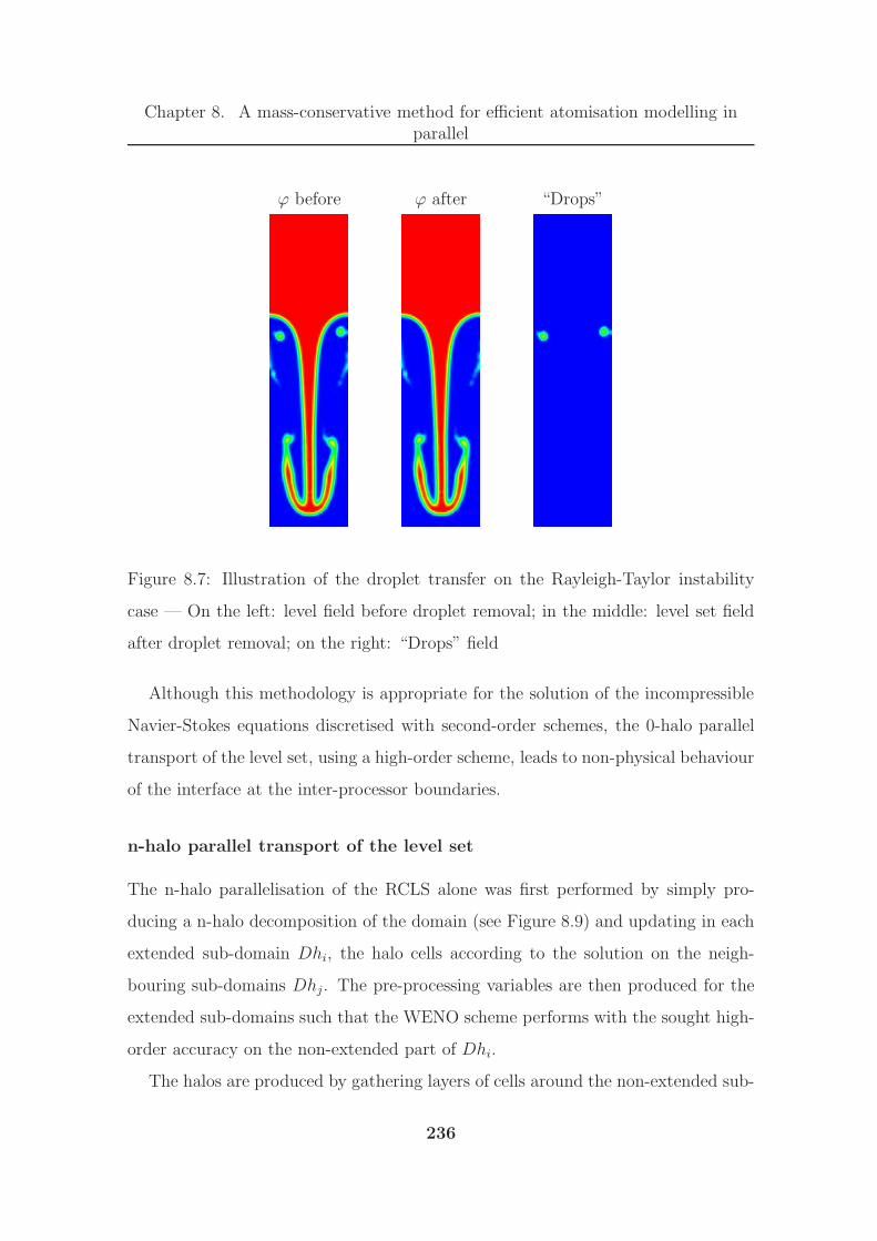
Chapter 8. A mass-conservative method for efficient atomisation modelling inparallel
ϕ before ϕ after “Drops”
Figure 8.7: Illustration of the droplet transfer on the Rayleigh-Taylor instability
case — On the left: level field before droplet removal; in the middle: level set field
after droplet removal; on the right: “Drops” field
Although this methodology is appropriate for the solution of the incompressible
Navier-Stokes equations discretised with second-order schemes, the 0-halo parallel
transport of the level set, using a high-order scheme, leads to non-physical behaviour
of the interface at the inter-processor boundaries.
n-halo parallel transport of the level set
The n-halo parallelisation of the RCLS alone was first performed by simply pro-
ducing a n-halo decomposition of the domain (see Figure 8.9) and updating in each
extended sub-domain Dhi, the halo cells according to the solution on the neigh-
bouring sub-domains Dhj. The pre-processing variables are then produced for the
extended sub-domains such that the WENO scheme performs with the sought high-
order accuracy on the non-extended part of Dhi.
The halos are produced by gathering layers of cells around the non-extended sub-
236

Chapter 8. A mass-conservative method for efficient atomisation modelling inparallel
Figure 8.8: Decomposition of the domain using a 0-halo approach [104] — On the
left the global domain; on the right the 0-halo sub-domains
domain Di. The number of layers Nl is a function of the order of the scheme and
is calculated such that the solution in the first layer of halo cells L1, is high-order
accurate. This ensures that the flux exchanged between Di and L1 is high-order
accurate, such that the solution is properly calculated in all the cells of the non-
extended part of Dhi.
However, the modelling capability involves not only the transport of the level set
but also the solution of the pressure-velocity coupling. As the incompressible Navier-
Stokes equations are discretised semi-implicitly (see Section 8.1.3), the resulting
system of algebraic equations (see Section 8.1.2) is solved by linear solvers. These
linear solvers are implemented in OpenFOAM for a 0-halo parallelisation and can
only run on a domain decomposed into non-overlapping domains.
n-halo parallel simulation of two-phase flows
An extension of the above n-halo methodology has been produced to transport
the level set with high-order accuracy and solve, in the same computation, the in-
237

Chapter 8. A mass-conservative method for efficient atomisation modelling inparallel
Figure 8.9: Decomposition of the domain using a n-halo approach — On the left the
global domain (0-halo inter-processor boundaries in black; extent of a n-halo sub-
domain in grey); on the right the 0-halo sub-domains Di (black line), the extended
sub-domains Dhi (blue line) and the halos (grey region)
compressible Navier-Stokes equations with the linear solvers implemented in Open-
FOAM.
Because of these linear solvers, the calculation has to run on a domain decomposed
with a 0-halo approach. In order to maintain the high-order accuracy of the level set
transport, the pre-processing variables are calculated on the extended sub-domains
and re-written for the 0-halo sub-domains. This re-writing process involves the
creation of Di-to-Dhi “maps” that relate the geometrical features of the 0-halo sub-
domains to their counterparts in the extended sub-domains Dhi. It also implies
generating new lists to store the mesh-dependent variables of the first layer of halo
cells L1. These variables are indeed required by the WENO scheme to perform
high-order calculations of the flux at the inter-processor boundaries.
At run time, the level set transport is performed on the 0-halo sub-domains.
However, as the re-written mesh-dependent variables refer to cells in the extended
238

Chapter 8. A mass-conservative method for efficient atomisation modelling inparallel
sub-domains, an intermediate “virtual field” ϕ is used to perform the operations of
the WENO scheme. This field is of the size of the extended sub-domains Dhi and is
populated with the level set scalar. The halo cells in ϕ are updated, through MPI
transfers, according to the level set field in the neighbouring 0-halo sub-domains.
The level set field ϕ is then calculated in the 0-halo sub-domain from the virtual
field ϕ.
As implemented in the code, the n-halo parallelisation involves the following
steps:
1. Decomposition of the global domain D into extended sub-domains Dhi.
2. Calculation of the mesh-dependent variables on the extended sub-domains.
At this step, both these pre-processing variables and some geometrical char-
acteristics of Dhi are written out to construct the Di-to-Dhi maps at a later
stage.
3. Decomposition of the global domain D into 0-halo sub-domains Di.
4. Construction of the Di-to-Dhi maps that relate the 0-halo sub-domains to the
extended sub-domains.
5. Re-writing of the pre-processing variables for Di using the Di-to-Dhi maps.
6. Parallel run of the computation using a virtual field ϕ to transport the level
set field ϕ with high-order accuracy.
Droplet transfer in parallel
Just like the rest of the modelling capability, the transfer of droplets has been
implemented in parallel. The parallel run of the algorithm on several processors
involves two specific cases: droplets spanning on several sub-domains and the re-
initialisation of the level set field ϕ on all cores simultaneously if a transfer of droplet
has occurred somewhere in the domain.
239
Chapter 8. A mass-conservative method for efficient atomisation modelling inparallel
As mentioned in Section 8.2.4, droplets spanning on several processors are ignored
by the selection algorithm. Therefore, these drops remain in the level set formulation
until they are convected well inside a sub-domain. The test that handles this case
checks that none of the cells of the droplet considered are on a processor boundary.
This test is made computationally efficient by producing, at pre-processing, lists of
inter-processor boundary cells for each sub-domain.
Depending on the flow field simulated, droplets may be removed from the level set
field in some sub-domains and not in others. However, it is crucial to synchronise
the re-initialisation of the hyperbolic tangent profile on all the processors or the
parallel computation will crash. This problem is mitigated by the creation of a list
of booleans storing the state of each sub-domain. Whenever, a droplet is removed
from ϕ in given sub-domain, its state is set to 1 — signifying the need for re-
initialisation — and an all-to-all transfer of the sub-domain states is performed.
The re-initialisation then occurs on each sub-domain as long as there is at least one
state set to 1 in the list.
8.4 Performance of the method on basic two-phase
flow problems
The calculations presented in this sub-section are typical tests that assess the per-
formance of the multiphase modelling capability. In particular, we present here the
results obtained by our method on two test cases: the Rayleigh-Taylor instability
and the falling drop in a pool. Through these simulations we illustrate four features
of our method:
• Accuracy,
• Robustness,
• Ability to run on different types of mesh,
240

Chapter 8. A mass-conservative method for efficient atomisation modelling inparallel
• Performance in parallel.
8.4.1 Rayleigh-Taylor instability
The settings for the simulation of the Rayleigh-Taylor instability are given Sec-
tion 4.2.2. For this test case, the transport of the volume fraction ϕ was performed
with our novel modelling capability (RCLSFoam) using the linear high-order scheme
and setting the interface thickness parameter to ǫ = 0.5∆x. This highlights the ro-
bustness of our method which copes with a density ratio of 7.4 (see Table 4.6)
without resorting to a WENO treatment of the discontinuity.
Ability to capture the physics
The relative performance of RCLSFoam with respect to OpenFOAM’s multiphase
flow solver (interFoam) is presented in Figure 8.10. This figure shows the solution
obtained by the two codes on the same triangular mesh made of 9234 cells, for six
different times in [0; 1.5] seconds.
The comparison of the interface predicted by the two solvers for the first three
times (t = 0.7s, 0.8s, 0.9s) demonstrates the superior performance of RCLSFoam
on asymmetrical meshes. Indeed, while the solution predicted by our modelling
capability remains close to the reference solution (see Gerris’ prediction on 256×1024
mesh Figure 4.5), OpenFOAM’s predictions are unrealistically asymmetrical. This
is probably due to the lower order of the numerical schemes used by interFoam
(smaller stencils) to transport the volume fractions. It suggests that interFoam is
not appropriate on general unstructured grids.
The solution predicted by interFoam for the last three times (t = 1.25s, 1.4s,
1.45s) illustrates a fundamental flaw of this solver. As already mentioned in Sec-
tion 4.2.2, interFoam produces non-physical wiggles in the stem of the mushroom-
shaped structure formed by the penetration of the denser phase into the lighter
phase. Figure 8.10 shows the build-up of these non-physical interfacial oscillations
241

Chapter 8. A mass-conservative method for efficient atomisation modelling inparallel
until they break the mushroom-shaped structure (see results for t = 1.45s).
Through various tests, we have identified that these non-physical features were
due to the compression flux implemented by Weller to maintain the sharpness of
the interface. However, this compression flux cannot be simply removed from in-
terFoam or Weller’s modelling tool would fall apart. As our modelling capability
maintains the interface sharp through the solution of the re-initialisation equation
(see Chapter 7), the Rayleigh-Taylor instability is correctly simulated. The ability
of RCLSFoam to model the Rayleigh-Taylor instability is particularly relevant to
the simulation of the atomisation process as this instability plays a significant role
in the primary breakup (see Chapter 2).
Handling of hybrid meshes
RCLSFoam’s ability to perform accurately on different types of grid is demon-
strated by comparing the solutions obtained on a triangular and a hybrid (triangles-
rectangles) mesh of similar size. Figure 8.11 shows the two meshes considered for
this study: a triangular mesh of 9234 cells and a hybrid grid of 8580 elements. The
rectangles of the hybrid mesh are distributed all along the width, in the middle
portion of the domain — where the interface is initialised — and the rest of the
domain is made of triangular elements.
Figure 8.11 presents the volume fractions and interface predicted by RCLSFoam
on the two meshes for five different times in [0; 1] second. As expected the results
obtained are very similar and, thanks to the high-order scheme implemented, the
method copes very well with the change of mesh type in the hybrid grid.
Small differences for the solution at time t = 1s can be perceived between the two
computations: the interface obtained on the hybrid mesh is slightly more symmet-
rical. This is due to the initialisation of the volume fraction field: whereas the sine
interface is set on a perfectly symmetrical Cartesian mesh for the hybrid grid, it is
initialised on a non-symmetrical mesh for the triangular grid. As the initialisation of
242
Chapter 8. A mass-conservative method for efficient atomisation modelling inparallel
the interface is critical to the symmetry of the solution, the results obtained on the
hybrid mesh are more symmetrical. it is also worth noting that the progression of
the mushroom-shaped structure in the triangular part of the hybrid mesh does not
affect its symmetry. This also illustrates how one can take advantage of the ability
to run on hybrid meshes and further highlights the relevance of this capability.
Mass conservation
In Chapter 6 and 7, a theoretical justification was given to attest that our numer-
ical transport of the smeared out liquid volume fraction leads to an exact mass
conservation. All the numerical experiments that we have performed in serial have
confirmed this assertion. In particular, we reported in Figure 8.12 the total mass
error observed for the simulation of the Rayleigh-Taylor instability on a triangular
mesh. These results confirmed that the RCLS conserves mass to machine accuracy
in serial.
Performance in parallel
As already mentioned in Section 8.3, OpenFOAM adopts a 0-halo approach to par-
allelisation. However, our modelling capability transports the volume fractions with
a high-order numerical scheme, such that a 0-halo parallel run with RCLSFoam
leads to non-physical solutions in the vicinity of the inter-processor boundaries. To
mitigate this issue we have implemented a n-halo parallelisation in OpenFOAM.
Figure 8.12 compares the predictions of the 0-halo and n-halo parallel computa-
tions of the Rayleigh-Taylor instability with the corresponding serial run. All three
calculations have been performed on the same triangular mesh made of 9234 ele-
ments and the predicted interface is given for five different times in [0; 1] second.
In order to highlight any disturbance caused by the parallelisation, the domain is
decomposed in four sub-domains by cutting half-way along the horizontal and ver-
tical directions. The domain decomposition associated to each parallel approach is
243

Chapter 8. A mass-conservative method for efficient atomisation modelling inparallel
overlaying the solution at time t = 0.2s in Figure 8.12.
The 0-halo parallel run presents non-physical features in the vicinity of the inter-
processor boundaries: distorted interface and inclusion of light phase in the cap
of the mushroom-shaped structure (see interface at times t = 0.8s, 0.9s, 1s). As
expected, the n-halo parallel run is free from non-physical features and matches
almost exactly the interface predicted by the serial run.
Through various tests, we have identified that the discrepancy between the serial
and the n-halo parallel run comes from a fundamental flaw in the parallel handling
of the pressure-velocity coupling in OpenFOAM. Unfortunately, this flaw affects the
mass conservation properties of the method in parallel.
NB: The n-halo parallel run of the RCLS method alone matches its serial counter-
part to machine accuracy.
As both interFoam and RCLSFoam conserve mass to machine accuracy when
running in serial, the impact of OpenFOAM’s flaw can be measured in terms of
mass variation over a computation. In particular, we have measured the absolute
variation of mass over a run of the Rayleigh-Taylor instability between the times
t = 0s and t = 1.5s: |∆m1.50 | (see the right most column in Figure 8.12).
The calculation of |∆m1.50 | confirms that RCLSFoam conserves mass to machine
accuracy in serial. However, with a 0-halo parallelisation, the absolute mass vari-
ation over the whole computation is O (10−3). Thanks to the implementation of a
n-halo parallel approach, this mass variation is reduced to O (10−8). As a frame of
reference, the parallel simulation of the Rayleigh-Taylor instability with interFoam
leads to an absolute variation of mass of: |∆m1.50 | = 1.94 × 10⁻⁶. With a mass
error two orders of magnitude smaller than interFoam’s, once again, our modelling
capability outperforms Weller’s code.
244

Chapter 8. A mass-conservative method for efficient atomisation modelling inparallel
8.4.2 Falling drop in a pool
The settings for the simulation of the falling drop in a pool are given Section 4.2.2.
For this test case, the transport of the volume fraction ϕ was performed with RCLS-
Foam using the WENO scheme and setting the interface thickness parameter to
ǫ = 0.5∆x. This computation is notoriously challenging as it involves a density
ratio of 816 (20 times larger than the density ratio encountered in aero-engines, see
tables 4.7 and 4.9).
For this computation, the solution of the pressure-velocity coupling is performed
using a Crank-Nicholson (CN) temporal discretisation and the resulting systems of
algebraic equations are solved with the generalised geometric-algebraic multi-grid
solver (GAMG). Although this choice of numerics generally improves the accuracy
(CN) and the speed (GAMG) of the computation, it significantly reduces the sta-
bility margin of the numerical method. As a result, the successful simulation of
the falling drop with such numerics is an achievement in itself. Indeed, no stable
computation were obtained for this test case with interFoam using either of these
numerical methods. This further highlights the superior robustness of our modelling
capability.
Figure 8.13 presents the volume fractions and the interface predicted by RCLS-
Foam on a 128× 256 Cartesian mesh for five different times in [0; 0.55] millisecond.
It can be seen in the Figure 8.13, that the RCLSFoam copes remarkably well with
the very large density ratio and that the results match closely the solution provided
by Gerris on the same mesh (see Figure 4.8).
To conclude, in this section we have demonstrated that our modelling capability
captures the physics well on any kind of unstructured grid. We also showed that
RCLSFoam conserves mass to machine accuracy in serial and to very high accu-
racy in parallel. In addition, we have established that this multiphase modelling
245

Chapter 8. A mass-conservative method for efficient atomisation modelling inparallel
tool is very robust. Finally, it follows from these numerical tests that RCLSFoam
outperforms interFoam in terms of accuracy, mass conservation and robustness.
246

Chapter 8. A mass-conservative method for efficient atomisation modelling inparallel
t = 0.7s t = 0.8s t = 0.9s t = 1.25s t = 1.4s t = 1.45s
interFoam
RCLSFoam
Figure 8.10: Interface predicted by RCLSFoam for the Rayleigh-Taylor instability
— Comparison RCLSFoam vs. interFoam
247

Chapter 8. A mass-conservative method for efficient atomisation modelling inparallel
t = 0.2s t = 0.7s t = 0.8s t = 0.9s t = 1s
Triangular
(9234 cells)
Hybrid
(8580 cells)
Figure 8.11: Volume fractions and interface (in black) predicted by RCLSFoam for
the Rayleigh-Taylor instability — Comparison hybrid vs. triangular mesh (meshes
overlaying the contours in white)
248

Chapter 8. A mass-conservative method for efficient atomisation modelling inparallel
t = 0.2s t = 0.7s t = 0.8s t = 0.9s t = 1s |∆m1.50 |
Serial 0
0-halo 4.58 × 10⁻³
n-halo 4.86 × 10⁻⁸
Figure 8.12: Interface predicted by RCLSFoam for the Rayleigh-Taylor instability
— Comparative performance of the 0-halo and n-halo parallel approaches
249

Chapter 8. A mass-conservative method for efficient atomisation modelling inparallel
t = 0s t = 0.15ms t = 0.2ms t = 0.35ms t = 0.55ms
Figure 8.13: Volume fractions and interface (in black) predicted by RCLSFoam for
the falling drop in a pool — Time t = 0s, 0.15ms, 0.2ms, 0.35ms, 0.55ms
250

Chapter 9
Simulation of liquid sheet breakup
The modelling capability as developed is applicable to both DNS and LES of atom-
isation. As our methodology relies on an implicit interface description method, the
breakup phenomenon is handled implicitly (no pinch off models) and its length scale
is of the order of the local grid size. As argued by Gorokhovski and Herrmann in [71],
although this makes the topology changes grid dependent, it does not significantly
affect the droplets larger than a few cell volumes.
To perform DNS, sufficient grid resolution has to be provided to capture the
Kolmogorov length scales in both phases, ηl and ηg, and the smallest liquid structure
produced ζ (typically drops at We = 10). As this is still infeasible in practice
for typical aero-engine conditions, it is necessary to resort to a “quasi-DNS/LES”
methodology [71].
In this chapter we present the sheet breakup of liquid fuel in co-flowing gas,
simulated using a quasi-DNS/LES methodology. The quasi-DNS/LES formulation
adopted for this calculation is described in Section 9.1, the settings of the computa-
tion are given in Section 9.2 and the results obtained with the modelling capability
(lesRCLSFoam) are presented in Section 9.3.
251

Chapter 9. Simulation of liquid sheet breakup
9.1 Quasi-DNS/LES formulation
This numerical framework involves applying a single-phase LES formulation in both
phases and extending it to the region of the interface. Due to the lack of established
models, this approach neglects the sub-grid scale effects associated with the presence
of the interface.
9.1.1 Filtering
As mentioned in Chapter 3, LES only resolves the larger scales of the turbulence
while the effect of the smaller scales are modelled. Therefore, the flow variables (u, p)
are decomposed into filtered components (u, p) and residual components (u′, p′),
according to:
u = u + u′ (9.1)
p = p + p′ (9.2)
Filter definition
The separation of the resolved scales from the sub-grid scales is performed by filtering
the flow variables [123]. Introducing the filter function G∆, its associated filter width
∆ (proportional to the smallest length scale resolved) and the computational domain
Ω, this filtering operation is defined by the following convolution [180, 211]:
u (x, t) = G∆ ∗ u =
∫∫∫
Ω
G∆ (r,x)u (x − r, t) dr (9.3)
where the filter kernel satisfies the normalisation condition:
∫∫∫
Ω
G∆ (r,x) dr = 1 (9.4)
The filter function G∆ defined above satisfies the following properties [211]:
252
Chapter 9. Simulation of liquid sheet breakup
1. Conservation of constants (equivalent to (9.4)). For a constant vector g this
property reads:
g = g (9.5)
2. Linearity. Introducing two vectorial space-time variables u and v, this condi-
tion reads:
u + v = u + v (9.6)
3. Commutation with differentiation. As G∆ is independent of time t (see (9.3)),
the filtering operation and the derivative with respect to time commute:
∂u
∂t=∂u
∂t(9.7)
In the case of an homogeneous filter: G∆ (r,x) = G∆ (r), the filtering operation
and the derivative with respect to the position commute:
∂ui∂xj
=∂ui∂xj
(9.8)
Although the decomposition of the flow variables into resolved and residual com-
ponents is analogous to a Reynolds decomposition, it is worth noting that the fil-
tered components (u, p) are random fields and that the filtered residual components(u′, p′
)are not systematically null. Therefore, in general, a filter (even homoge-
neous) is not a “Reynolds operator” [211] and:
u 6= u (9.9)
u′ 6= 0 (9.10)
uu 6= uu (9.11)
Non-uniform filter width
A filter can only be considered homogeneous on a uniform grid. In the case of un-
structured grids, the filter width is a function of space ∆ = ∆ (x) and a commutation
error appears. By choosing carefully the filter kernel G∆, Vasilyev et al. showed that
253
Chapter 9. Simulation of liquid sheet breakup
it is possible to control the order of this error on unstructured grids [82, 147, 265].
However, this approach involves explicit filtering which can be cumbersome and
computationally expensive [43].
After Villiers, we choose to minimise the commutation error by smoothing the
distribution of filter widths [43]. For each element Ei of the mesh, a “cell-derived”
filter width ∆Eican be calculated as a function of the cell volume |Ei|:
∆Ei= 3√|Ei| (9.12)
Let us note ∆i the filter width of Ei. Instead of setting directly ∆i = ∆Ei, the prin-
ciple of the smoothing method is to increase the filter width of the cells neighbouring
larger control volumes [43]. For this purpose, a fixed gradient for the smoothed dis-
tribution is defined — based on a coefficient C∆ — such that ∆i ≥ ∆Ei. Introducing
the set of cells neighbouring Ei: Ni =⋃j Ej, the smoothing scheme reads:
∆i = maxj∈Ni
(∆Ei
,∆Ej
C∆
)(9.13)
As recommended by Villiers, we have set the smoothing coefficient to:
C∆ = 1.1 (9.14)
In his numerical experiments, Villiers observed that the smoothing approach was
sufficient to obtain relatively good results at a fairly low cost.
9.1.2 Filtered Navier-Stokes equations
The convolution of (8.1) and (8.2) with an homogeneous kernel filter G∆ provides
the following filtered incompressible Navier-Stokes equations:
∇ · u = 0 (9.15)
∂ (ρu)
∂t+ ∇ · (ρu ⊗ u) = −∇p+ ρg + σκ∇ϕ+ ∇ ·
(2µD − ρT
)(9.16)
where:
254

Chapter 9. Simulation of liquid sheet breakup
• The filtered rate-of-strain tensor D reads:
D =1
2
(∇u + (∇u)T
)(9.17)
• T is the residual-stress tensor:
T = u⊗ u− u⊗ u (9.18)
• Following the principle of the quasi-DNS/LES approach, the sub-grid scale
contributions of the capillary forces (fcap)SGS have been neglected:
(fcap)SGS = 0 = σκ∇ϕ− σκ∇ϕ (9.19)
σκ∇ϕ = σκ∇ϕ (9.20)
Leonard proposed the following decomposition of the residual-stress tensor:
T =(u ⊗ u − u ⊗ u
)+(u ⊗ u′ + u′ ⊗ u
)+(u′ ⊗ u′
)
= L + C + R (9.21)
where the Leonard-stress tensor L represents the “interactions among the large
scales”, the cross-stress tensor C reflects the “interactions between large and small
scales” and the SGS Reynolds-stress tensor R stands for “the interactions between
sub-grid scales” [211].
9.1.3 Residual kinetic energy
Filtering the kinetic energy field E = 12u · u produces E:
E =1
2u · u (9.22)
Decomposing E into the kinetic energy of the filtered velocity field Ef and the
residual kinetic energy kr leads to [180]:
E = Ef + kr (9.23)
255

Chapter 9. Simulation of liquid sheet breakup
where kr is expressed as:
kr =1
2u · u − 1
2u · u (9.24)
Noting that kr = 12tr (T ), the decomposition of the residual-stress tensor into an
isotropic part and a deviatoric part TD can be expressed as follows:
T =2
3krI + TD (9.25)
where I is the unit tensor.
9.1.4 Sub-grid scale modelling
For this computation, we have chosen to model the sub-grid scale stress tensor Twith the constant coefficient one-equation eddy-viscosity model (OEEVM) proposed
by Yoshizawa [281].
Eddy-viscosity assumption
The OEEVM is based on Boussinesq’s eddy-viscosity concept which postulates that
the mechanism governing the transfer of energy from the resolved scales to the
residual scales is analogous to the mechanism driving the molecular diffusion. With
this hypothesis, the deviatoric part of the residual-stress tensor TD is assumed locally
aligned with the deviatoric part of the filtered rate-of-strain tensor DD and the
normal stresses (considered isotropic) are calculated from the residual kinetic energy
kr [64]. Introducing the eddy-viscosity of the residual motions νr, Boussinesq’s
assumption leads to the following expression for the residual-stress tensor:
T =2
3krI − 2νrDD (9.26)
However, as the flow is considered incompressible, the filtered dilatation is null:
d = tr(D)
= ∇ · u = 0 (9.27)
Such that:
D = DD +1
3dI = DD (9.28)
256

Chapter 9. Simulation of liquid sheet breakup
It follows that SGS eddy-viscosity type models for incompressible flows express the
residual-stress tensor as the following function of kr and νr:
T (kr, νr) =2
3krI − 2νrD (9.29)
The algebraic eddy-viscosity model of Smagorinsky [234] calculates directly the
parameters kr and νr from the characteristic filtered rate of strain: D =(2D : D
)
by assuming that the rate of production of the residual kinetic energy is exactly
balanced by the rate of dissipation of kinetic energy. As this balance breaks down
near walls and in jets and wakes, Yoshizawa proposed a model equation for the
residual kinetic energy kr.
Transport equation for the residual kinetic energy
The exact transport equation for kr (TK) can be obtained by combining the mo-
mentum equation (ME) (given by (8.2)) and its filtered counterpart(ME
)(given
by (9.16)) in the following way [41]:
(TK) : u · (ME) − u ·(ME
)
Neglecting the terms related to the capillary forces in (TK) leads to the following
equation for the residual kinetic energy [41]:
∂kr∂t
+ ∇ · (ukr)︸ ︷︷ ︸
Convection
= −∇ ·(
1
2(u · u)u − E u +
1
ρpu− 1
ρpu− u · T
)+ ∇ · (ν∇kr)
︸ ︷︷ ︸Diffusion
− ν(∇u : ∇u−∇u : ∇u
)︸ ︷︷ ︸
Dissipation
−D : T︸ ︷︷ ︸Production
(9.30)
Yoshizawa derives a model transport equation for the residual kinetic energy by
using the statistical results from the direct-interaction approximation [114–116]. As
this statistical approach assumes the distinct separation of the grid-scales mean
motions and the sub-grid scale fluctuating motions [280, 282], the Leonard-stress
tensor L and the cross-stress tensor C are neglected.
257
Chapter 9. Simulation of liquid sheet breakup
Noting Dkrthe non-molecular diffusion term in (9.30) and εkr
the dissipation
term in (9.30), Yoshizawa’s statistical framework leads to the following models for
Dkrand εkr
:
Dkr= ∇ · (νr∇kr) (9.31)
εkr=Cǫk
32r
∆(9.32)
with the following expression for the eddy-viscosity of the residual motions:
νr = Cνk12r ∆ (9.33)
As a result, the model transport equation for the residual kinetic energy reads:
∂kr∂t
+ ∇ · (ukr) = ∇ · ((νr + ν)∇kr) − εkr−D : T (9.34)
The same model equation for the transport of kr was derived by Schumann using
dimensional analysis [220].
Yoshizawa recommends the model parameters Cν ≃ 0.05 and Cε ≃ 1. Building
upon the successful application of this SGS model to the simulation of diesel jet
atomisation by Villiers et al., we will use the following values for Cν and Cε [44]:
Cν = 0.07 (9.35)
Cε = 1.05 (9.36)
Performance of the OEEVM
As intended, this model performs better than the Smagorinsky model in regions of
the flow where the balance between production and dissipation breaks down: wakes,
jets and near-wall flows. And wherever the production-dissipation equilibrium is
valid the OEEVM revert to the Smagorinsky model [64].
However, as the eddy-viscosity concept assumes the isotropy of the normal resid-
ual stresses, the OEEVM requires a high mesh density in near-wall regions to capture
258
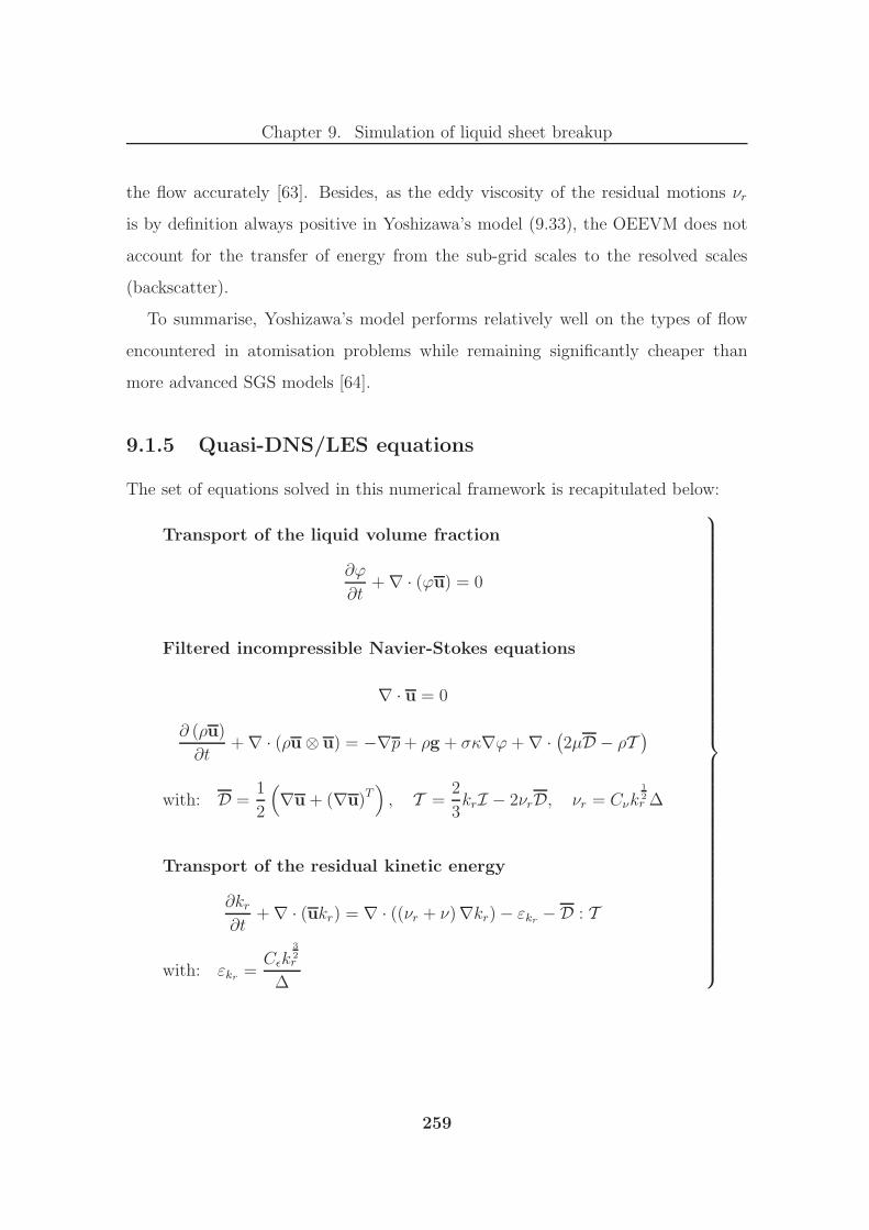
Chapter 9. Simulation of liquid sheet breakup
the flow accurately [63]. Besides, as the eddy viscosity of the residual motions νr
is by definition always positive in Yoshizawa’s model (9.33), the OEEVM does not
account for the transfer of energy from the sub-grid scales to the resolved scales
(backscatter).
To summarise, Yoshizawa’s model performs relatively well on the types of flow
encountered in atomisation problems while remaining significantly cheaper than
more advanced SGS models [64].
9.1.5 Quasi-DNS/LES equations
The set of equations solved in this numerical framework is recapitulated below:
Transport of the liquid volume fraction
∂ϕ
∂t+ ∇ · (ϕu) = 0
Filtered incompressible Navier-Stokes equations
∇ · u = 0
∂ (ρu)
∂t+ ∇ · (ρu ⊗ u) = −∇p+ ρg + σκ∇ϕ + ∇ ·
(2µD − ρT
)
with: D =1
2
(∇u + (∇u)T
), T =
2
3krI − 2νrD, νr = Cνk
12r ∆
Transport of the residual kinetic energy
∂kr∂t
+ ∇ · (ukr) = ∇ · ((νr + ν)∇kr) − εkr−D : T
with: εkr=Cǫk
32r
∆
259
Chapter 9. Simulation of liquid sheet breakup
9.2 Settings of the computation
Previous numerical studies of atomisation have highlighted the sensitivity of the
computation to boundary conditions (see Chapter 5). This section details the choices
made in this demonstration exercise. In particular, the mechanical and physical
boundary conditions are given in Section 9.2.1 and in Section 9.2.2 we present a
parametric study of the RCLS method which leads to the choice of settings for the
computation.
9.2.1 Domain and material properties
In Chapter 4, we reproduced the results obtained by Villiers et al. for the simulation
of Diesel jet atomisation [44]. We then extended this approach (similar physical
properties and domain dimensions) to the computation of liquid sheet breakup in
co-flow (see Section 4.3.2).
In order to demonstrate the modelling capability on a test case reproducing the
breakup mechanisms observed at aero-engine conditions, we have chosen to compute
the flat sheet breakup at We = 9300.
Computational domain
The computational domain generated for this simulation is a cuboid of 3 × 1 × 1
mm3, meshed with 2.36×10⁶ cells. In order to demonstrate the capability on general
polyhedral meshes, the grid is made of 8.07 × 10⁵ hexahedra, 1.5 × 10⁶ tetrahedra
and 5.4 × 10⁴ pyramids (see bottom picture in Figure 9.1).
The gas and fuel injection channels are modelled — they span over 1mm in
the longitudinal direction — and the thickness of the plates separating the injec-
tion channels is resolved (see top picture in Figure 9.1). Both of these features
have proven to be of significant importance in the numerical simulation of primary
breakup (see [65]). The geometrical details of the injection configuration can be
found in the “Flat sheet” column of Table 4.11.
260

Chapter 9. Simulation of liquid sheet breakup
Domain and boundary conditions
Mesh along the centreplane (z = 0)
Figure 9.1: Computational domain for the simulation of atomisation — In the top
half: the mesh of the back plane (edges in blue) and the boundaries (walls in grey,
fuel inlet in blue and gas inlets in red) are pictured
The front and back planes — respectively defined by z = 0.5 and z = −0.5 (see
top picture in Figure 9.1) — are set as symmetric boundary condition. The plane at
261

Chapter 9. Simulation of liquid sheet breakup
x = 0 is the inlet of the computational domain. In the central part of this plane —
between the two plates — the fuel (ϕ = 1) is injected at a speed of 2ms−1. Above
and below the fuel injection channel, the gas (ϕ = 0) enters the domain at a speed of
40ms−1. The rest of the boundaries are defined as inlet/outlet boundary conditions.
In order to take advantage of the ability to run on hybrid meshes, structured
hexahedral grids have been fitted around walls. Similarly, to improve the accuracy
of the atomisation modelling, the regions where the breakup is expected to occur
have been meshed with hexahedral cells. Because of the instability of the inlet/outlet
boundary conditions in OpenFOAM, these boundaries have also been meshed with
hexahedra. The rest of the domain is composed of tetrahedra and pyramids. The
pyramidal mesh consists of a single layer of cells performing the transition between
the hexahedral and the tetrahedal meshes.
In the resulting mesh, the smallest edge length is ∆xmin = 5µm and the average
characteristic length scale of the grid (as defined in (9.38)) is ∆x = 8.4µm.
Material properties
Although the material properties chosen for this study (see Table 4.9) differ slightly
from those of an aero-engine, the physical quantities remain similar. The non-
dimensional numbers related to this computation are given in Table 9.1 and the
smallest length scales associated with the flow field are reported in Table 9.2.
Considering that a given length scale η is resolved if η ≥ 2∆x, it can be seen
in Table 9.2 that only the Kolmogorov length scale in the liquid phase ηliq is prop-
erly resolved by the mesh. This justifies the use of a sub-grid scale model for the
turbulence in the gas phase.
Table 9.2 also suggests that the mesh is far from resolving the smallest liquid
structures produced. This further highlights the need to develop sub-grid scale
models for multiphase flows.
262

Chapter 9. Simulation of liquid sheet breakup
Table 9.1: Non-dimensional numbers associated to the flow simulated
Reliq 67
Regas 18800
We 9300
Oh 7.55 × 10⁻²
Table 9.2: Smallest length scale of the flow field — Assuming a turbulence intensity
of 5% in the liquid and 10% in the gas
Liquid phase Kolmogorov scale, ηliq 81µm
Gas phase Kolmogorov scale, ηgas 1.4µm
Droplet diameter at We = 10, dWe=10 0.22µm
Minimum mesh size, ∆xmin 5µm
Average mesh size, ∆x 8.4µm
263

Chapter 9. Simulation of liquid sheet breakup
9.2.2 Choice of RCLS settings
The RCLS method involves the following parameters:
• The order of the polynomial reconstruction of the high-order scheme: r.
• The type of high-order scheme: linear or WENO.
• The coefficient controlling the thickness of the interface ǫ.
• The periodicity of the re-initialisation.
Although our numerical scheme can formally reach arbitrarily high order in space,
in this demonstration of the modelling capability we limit ourselves to a third-order
polynomial reconstruction: r = 3.
This leads to a third-order accurate linear scheme for the transport of the liquid
volume fraction and in the case of a WENO reconstruction, the scheme is typi-
cally fourth-order accurate. In the interest of robustness and because atomisation
problems involve large density ratios, we choose to use the WENO scheme for this
calculation.
As mentioned in Section 7.2.4, the coefficient ǫ affects the stability of the method
and — through the interface thickness — controls the resolution of the interface
geometry. This coefficient is defined as a function of the mesh size (see (7.40)), such
that on general unstructured meshes, ǫ varies from cell to cell. However, for our
simulation, we will take ǫ uniform on the whole computational domain Ω:
ǫ = C∆x (9.37)
where C is a constant coefficient.
Introducing the number of internal faces of the mesh: NFIΩ and, for a given face
Fl noting the cell centres of the owner and neighbour cells respectively Ol and Nl,
∆x is given by:
∆x =1
NFIΩ
NF IΩ∑
l=1
|−−→OlNl| (9.38)
264

Chapter 9. Simulation of liquid sheet breakup
As demonstrated in Section 7.2.4, the method’s stability requires C ≥ 0.5 when ǫ is
defined as a function of the local mesh size ∆x.
Another parameter of conservative level set methods was introduced by Des-
jardins et al. in [47]: the periodicity of the re-initialisation. In numerical tests,
the authors noted that an optimum value could be found for this parameter. In
particular, they observed that re-initialising the level set profile less frequently (up
to a certain point) would lead to a better resolution of thin ligaments.
Scope of the parametric study
In this paragraph, a parametric study of the RCLS method is presented. The param-
eters considered are the CLS coefficient ǫ and the number of time steps Ns between
two re-initialisations of the hyperbolic tangent profile. The relative performance of
the method is assessed on the following test cases (defined in Section 4.2.1): Zale-
sak’s slotted disk (1282 Cartesian mesh) and the disk in a deformation field (2562
Cartesian mesh). Both of these test cases are performed on Cartesian grids, such
that the definitions of ǫ in (7.40) and in (9.37) are equivalent.
In this parametric study, we tested the RCLS with the following parameters:
• C = 0.5, 1.0 (see Figure 9.2).
• Ns = 1, 5, 10 and no re-initialisation (see Figure 9.3).
Figures 9.2 and 9.3 present the results obtained for:
• Zalesak’s slotted disk (middle column), referred to as “Zalesak” in the figures.
The contour plots of the scalar transported ϕ are given at t = 1s (after one
circular translation) and the predicted level sets ϕ = 0.05, 0.5, 0.95 are shown
in black. It is worth recalling that the level set ϕ = 0.5 represents the approx-
imate location of the phase boundary and that the inner-most (ϕ = 0.95) and
outer-most (ϕ = 0.05) contour lines gather 90% of the phase transition.
265

Chapter 9. Simulation of liquid sheet breakup
• The disk in a deformation field (right column), referred to as “Spiral” in the
figures. The level set contours ϕ = 0.5 obtained at t = 3s are drawn in blue.
Choice of ǫ
As expected, when the interface is thickened the method’s ability to capture thin
ligaments worsens (see right column in Figure 9.2). However, increasing ǫ stabilises
the method (see Section 7.2.4) and smooths the level set contours (see middle column
in Figure 9.2).
Also, bearing in mind that the RCLS method is part of a bigger modelling capa-
bility, setting the coefficient C to larger values leads to diffused droplets. Although
the droplet transfer methodology is designed to cope with such situations, allowing
the drops to diffuse unreasonably would result in the over-prediction of coalescence
events. In addition, from a physical point of view it is generally desirable to limit
the spread of the phase transition as it is the locus of the capillary forces (CSF
formulation, see Chapter 3).
From the parametric study, it seems that better results are obtained with C = 0.5.
Although this value constitutes the limit of stability, the cells of the unstructured
computational domain have a low aspect ratio (see Section 9.2.1) and the robustness
of the method is maintained with ǫ = 0.5∆x for this mesh.
Choice of Ns
Increasing the periodicity of the re-initialisation step improves the ability of the
method to capture thin ligaments (see right column in Figure 9.3). This im-
provement is limited by a maximum value for Ns as the pure advection of ϕ (no-
reinitialisation: Ns −→ ∞) is clearly sub-optimal.
Although the largest periodicity tested (Ns = 10) provides the best results in
terms of ligament length, it leads to convoluted contours of the level set ϕ = 0.95
for Zalesak’s slotted disk. Once again, as the surface tension is applied in the region
266

Chapter 9. Simulation of liquid sheet breakup
Zalesak Spiral
ǫ = 0.5∆x
ǫ = 1.0∆x
Figure 9.2: Effect of the coefficient ǫ on the performance of the RCLS — Results
for C = 0.5, 1.0 with Ns = 5
of the phase transition, it is desirable to limit the spread of the phase transition and
to maintain the regularity of the level set contours.
For this reason, we choose to re-initialise the hyperbolic tangent profile every five
time steps: Ns = 5. This periodicity gives results similar to the solution performed
with Ns = 1 at a much lower computational cost (∼ 25% faster for the translation
of the slotted disk).
267

Chapter 9. Simulation of liquid sheet breakup
Zalesak Spiral
No re-initialisation
Ns = 1
Ns = 5
Ns = 10
Figure 9.3: Effect of the periodicity of re-initialisation on the performance of the
RCLS — Results for Ns = 1, 5, 10 and no re-initialisation with C = 0.5
268

Chapter 9. Simulation of liquid sheet breakup
Summary
The parameters of the RCLS have been chosen to reach a better trade-off in terms of
performance of the RCLS, stability of the method and compliance with the physics
of the atomisation. A finer tuning of the method — with a non-uniform value of ǫ
in the computational domain — may be performed as a follow-on research project.
The chosen set of RCLS parameters is recapitulated in Table 9.3.
Table 9.3: RCLS parameters for the simulation of atomisation
Order of the polynomial reconstruction: r = 3
Numerical scheme: WENO
CLS coefficient: ǫ = 0.5∆x
Periodicity of the re-initialisation: Ns = 5
269
Chapter 9. Simulation of liquid sheet breakup
9.3 Results and discussion
As the emphasis of this numerical study is placed on the mechanisms driving the
primary breakup, the computational domain is limited to the close vicinity of the
injection plane. Consequently, no droplet characteristics have been extracted from
this calculation.
9.3.1 Instabilities of the liquid sheet
The stability analysis performed for a liquid sheet in co-flow [12, 38] demonstrated
that the breakup involved undulations of the liquid sheet in sinuous and varicose
modes.
In order to illustrate the mechanisms of the sheet breakup, we have extracted
the interface contour in both a longitudinal plane Pl and a transverse plane Pt
of the computational domain (both passing through the centre of the domain, see
Figure 9.4). These interface contours are given in Figure 9.5 for Pl and in Figure 9.6
for Pt.
Although the interface contours in the longitudinal and transverse planes present
different shapes and set of modes, it is clear from Figure 9.5 and Figure 9.6 that
the liquid fragmentation is highly non-linear and that the undulations of the sheet
involve sinuous and varicose modes in both directions.
As predicted by the theory, our simulation shows — in both the longitudinal and
the transverse planes — the initial growth of a sinuous mode: the fundamental of
the sheet undulation. Harmonic waves then develop on top of the sinuous oscillation
mode of the two surfaces of the sheet. The first harmonic being of varicose type, the
growth of the harmonic waves leads to the thinning of the sheet, thus facilitating
the breakup of the sheet through aerodynamic tearing (see Figure 9.5).
270

Chapter 9. Simulation of liquid sheet breakup
Figure 9.4: Planes of interface contour extraction — In red: the outline of Pl;
in green: the interface contour in Pl; in blue: the outline of Pt; in orange: the
interface contour in Pt
271

Chapter 9. Simulation of liquid sheet breakup
t = 0.835ms t = 0.91ms
t = 0.935ms t = 1.08ms
Figure 9.5: Interface contour in the longitudinal plane — Time t =
0.835ms, 0.91ms, 0.935ms, 1.08ms
272
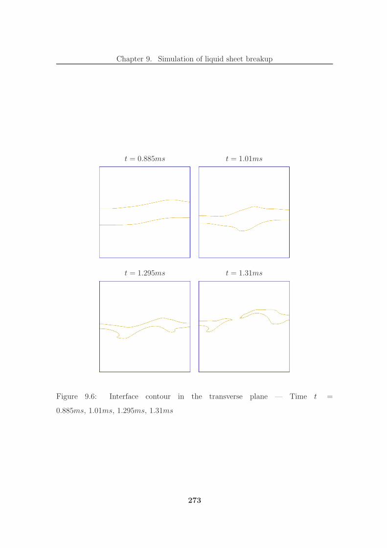
Chapter 9. Simulation of liquid sheet breakup
t = 0.885ms t = 1.01ms
t = 1.295ms t = 1.31ms
Figure 9.6: Interface contour in the transverse plane — Time t =
0.885ms, 1.01ms, 1.295ms, 1.31ms
273

Chapter 9. Simulation of liquid sheet breakup
9.3.2 Torn sheet breakup
Sheet breakup regimes
Fernandez et al. studied the breakup of a flat sheet of water (300µm thick, Uliq ∈[1; 2] ms−1) sheared on either side by a stream of gas (Ugas ∈ [20; 70] ms−1, pgas ∈[1; 6] bar). In their experimental analysis [56], the authors classify the regime of the
primary breakup according to the momentum flux ratio M (see (2.2)). In particular,
they identify three regimes of liquid sheet breakup:
Up to M = 0.5: The cellular breakup. This regime is characterised by the forma-
tion of cell-like structures in the liquid sheet through the build-up of longitu-
dinal and transverse undulations of similar wavelength. Such a combination
of undulations leads to the bursting of the membranes associated with the
cell-like structures and to the creation of spanwise ligaments.
From M = 0.5 to M = 5 The stretch streamwise ligament breakup. Similarly to
the cellular breakup, this regime involves the build-up of both longitudinal
and transverse undulations. However, for this regime the fragmentation of
the sheet occurs along the longitudinal direction such that the bursting of the
membranes is accompanied with the creation of streamwise ligaments.
Above M = 5: The torn sheet breakup. As for the previous breakup regime, the
torn sheet breakup produces droplets through the disintegration of membranes
and via the fragmentation of streamwise ligaments. However, the streamwise
ligaments formed have highly irregular shapes and disintegrate through aero-
dynamic tearing rather than Plateau-Rayleigh instability. This regime also
involve the tearing of the continuous region of the liquid sheet into large liquid
structures further fragmented by the aerodynamic forces.
In our simulation of the primary breakup, the momentum flux ratio is: M = 9.5.
According to the above classification, this value of M puts the calculation in the
274

Chapter 9. Simulation of liquid sheet breakup
regime of torn sheet breakup. The flow features predicted by our simulation for this
breakup regime are reported in figures 9.7 to 9.11.
Interaction with vortices
The figures of this sub-section present the liquid phase together with an ad hoc
iso-surface of the Q-criterion [97] to illustrate the interaction of the turbulence with
the liquid sheet. The Q-criterion — defined as the second invariant of the velocity
gradient tensor — is widely used to visualise the coherent vortical structures in the
flow field [46, 48]. The scalar field Q is given by:
Q =1
2
((tr (∇u))2 − tr (∇u · ∇u)
)(9.39)
Due to the difference in velocity between the two phases, a shear layer appears
on the interface. As a result, a Kelvin-Helmoltz (KH) instability builds up and
— as can be seen in figures 9.7 to 9.11 — KH rollers form on either side of the
liquid sheet, following initially the shape of the phase interface. As these vortices
progress through the computational domain, they break up, thus increasing the
level of turbulence downstream of the liquid bulk. In particular, the figures presented
illustrate the breakup of vortices through their interaction with the liquid structures.
Evolution of the liquid sheet
The simulation of sheet breakup involves three main phases:
• The build-up of instabilities on the two interface surfaces (t < 0.935ms).
• The flapping of the sheet in the longitudinal and transverse directions (t ∈[0.935; 1.25] ms).
• The tearing of the liquid sheet (t > 1.25ms).
275
Chapter 9. Simulation of liquid sheet breakup
Build-up of instabilities This phase starts with the penetration of the liquid
in the computational domain and finishes with the first occurrence of the breakup
at t = 0.935ms. It involves the initial deformation of the interface in the injection
channel and the development of sinuous and varicose modes of undulation of the
liquid sheet (see Figure 9.7). As described in Section 9.3.1, the growth of surface
waves — in both the longitudinal and the transverse directions — leads to the
thinning of the liquid sheet, thus facilitating the first pinch-off event by aerodynamic
tearing.
Sheet flapping This phase involves the flapping of the sheet in both the longitu-
dinal and the transverse directions, similarly to a flag. For this stage, the simulation
predicts the disintegration of the membranes formed at the peaks and the troughs
of the undulations (see Figure 9.8). The membrane puncturing is accompanied by
the formation and the pinch-off of streamwise ligaments (see Figure 9.9). These flow
features suggest that the breakup regime is the stretch streamwise ligament breakup.
It constitutes a transition before the establishment of the torn sheet breakup.
Sheet tearing From t = 1.25ms, the computation predicts the tearing of the
sheet in the transverse and then the longitudinal directions (see Figure 9.10 and
Figure 9.11 respectively).
At t = 1.25ms, the liquid sheet presents a bag-like structure bent towards the top
of the domain. As the sheet significantly obstructs the gas stream, it is subjected to
relatively high aerodynamic forces and a tear is initiated. While the tear propagates
in the transverse direction — following the path of minimum sheet thickness — the
liquid structure being torn away undergoes a membrane-type breakup.
Then, at time t = 1.3ms, a bag-like structure is formed in the centre of the
sheet. This structure is punctured and the aerodynamic forces initiate a longitudinal
tear in the hole produced. As the tear propagates upstream in the liquid phase,
two streamwise ligaments are formed. These ligaments develop bag-like structures
276
Chapter 9. Simulation of liquid sheet breakup
themselves and get subsequently torn away by the gas stream.
The flow field predicted by the numerical simulation in the “sheet tearing” phase,
matches closely the description of the torn sheet breakup given in [56]. This validates
qualitatively our simulation of the liquid sheet breakup.
Our computation of the liquid sheet breakup highlights the potential of the nu-
merical approach to study the mechanisms of the primary breakup. Indeed, the
simulation described the entire breakup process while the stability analysis could
only predict its onset and experiments could only capture the sheet tearing. In
addition, only the CFD can provide insight on the interaction of the vortices in the
gas phase with the liquid structures.
9.3.3 Breakup length
As a first step towards a quantitative validation of this numerical simulation of sheet
breakup, the average breakup length predicted by the computation is compared to
the value given by the correlation provided in [56].
In [56], Fernandez et al. relate the breakup length Lb to a non-dimensional
number. Recalling that h is the height of the fuel injection channel and noting Weh,
the Weber number based on h, this relation reads:
Lbh
= f
3
√Uliq
Ugas
MWeh
(9.40)
For the conditions of the calculation, the non-dimensional number is equal to
0.008, which leads to Lb
h= 6 ± 2. In our numerical experiment, we observe an
average breakup length of Lb
h= 5 which is well within the range predicted by the
correlation.
It is also worth noting that (9.40) is based on a restricted range of flow conditions
(water liquid sheet ; air pressure below 6bar), and that it accounts for a limited range
277

Chapter 9. Simulation of liquid sheet breakup
of parameters (ignores Reliq). A correlation based on a more exhaustive experimental
test campaign may further confirm the prediction of our simulation.
278

Chapter 9. Simulation of liquid sheet breakup
t = 0.72ms t = 0.81ms
t = 0.835ms t = 0.86ms
t = 0.91ms t = 0.935ms
Figure 9.7: Simulation of flat sheet breakup with lesRCLSFoam — Liquid phase (in
grey) and an ad hoc iso-surface of Q-criterion (in transparent red) for the build-up
of instabilities
279
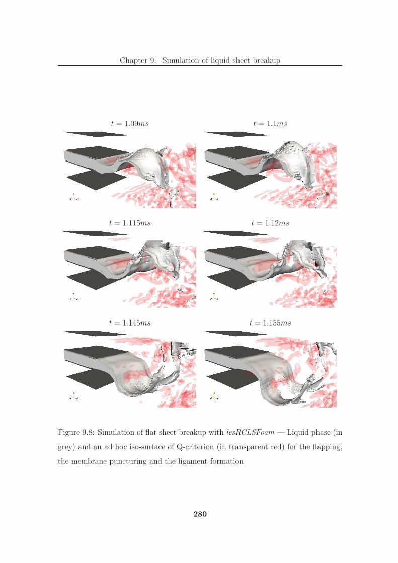
Chapter 9. Simulation of liquid sheet breakup
t = 1.09ms t = 1.1ms
t = 1.115ms t = 1.12ms
t = 1.145ms t = 1.155ms
Figure 9.8: Simulation of flat sheet breakup with lesRCLSFoam — Liquid phase (in
grey) and an ad hoc iso-surface of Q-criterion (in transparent red) for the flapping,
the membrane puncturing and the ligament formation
280
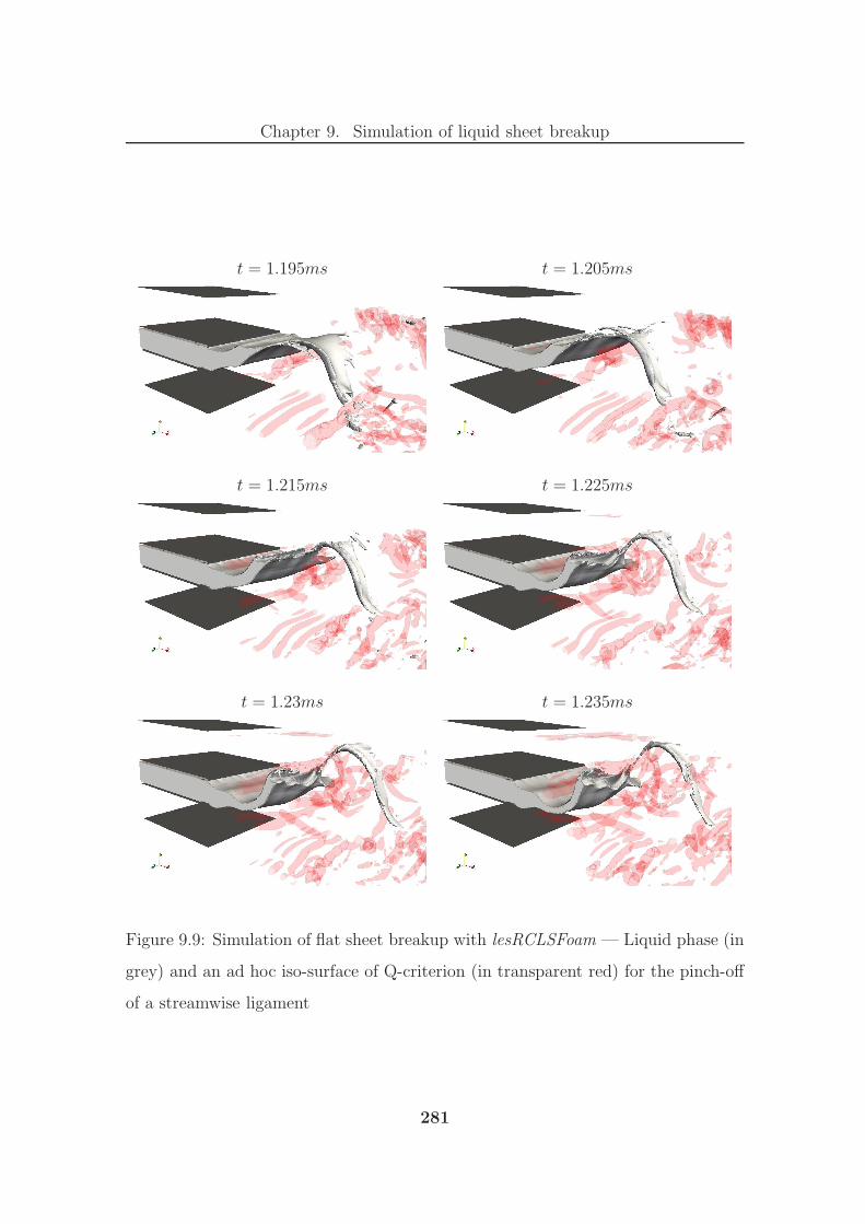
Chapter 9. Simulation of liquid sheet breakup
t = 1.195ms t = 1.205ms
t = 1.215ms t = 1.225ms
t = 1.23ms t = 1.235ms
Figure 9.9: Simulation of flat sheet breakup with lesRCLSFoam — Liquid phase (in
grey) and an ad hoc iso-surface of Q-criterion (in transparent red) for the pinch-off
of a streamwise ligament
281

Chapter 9. Simulation of liquid sheet breakup
t = 1.25ms t = 1.265ms
t = 1.27ms t = 1.28ms
t = 1.29ms t = 1.295ms
Figure 9.10: Simulation of flat sheet breakup with lesRCLSFoam — Liquid phase
(in grey) and an ad hoc iso-surface of Q-criterion (in transparent red) for the tearing
of the sheet in the transverse direction
282

Chapter 9. Simulation of liquid sheet breakup
t = 1.3ms t = 1.315ms
t = 1.325ms t = 1.335ms
t = 1.355ms t = 1.37ms
Figure 9.11: Simulation of flat sheet breakup with lesRCLSFoam — Liquid phase
(in grey) and an ad hoc iso-surface of Q-criterion (in transparent red) for the tearing
of the sheet in the longitudinal direction
283
Chapter 10
Conclusion
The main accomplishment of this work consists in the generation of a modelling
capability for the parallel computation of the fuel injection in aero-engine combustion
chambers. To reach this goal, a modelling strategy has been produced based on the
existing methodologies in the field of multiphase CFD and the requirements of the
aeronautical industry. This set of guidelines lead to the creation of a novel WENO
scheme for general polyhedral meshes, the development of a robust conservative
level set method to transport the interface and the generation of an algorithm to
output droplet boundary conditions to combustion codes. In this chapter the main
achievements of this research project are summarised in Section 10.1 and some
follow-on research topics are suggested in Section 10.2.
10.1 Achievements
10.1.1 Modelling strategy to simulate fuel injection
A comprehensive literature review has been produced, reporting the current physical
description of the phenomenon and a broad overview of the numerical methods avail-
able to simulate multiphase flows. In particular, the existing numerical frameworks,
the various interface description methods and the means of handling the singulari-
284

Chapter 10. Conclusion
ties introduced by the interface are described in detail. Finally, the state-of-the-art
methods developed by scientists to simulate the atomisation process are presented
and the current trends in atomisation modelling are outlined.
Also, two open source multiphase codes have been identified: OpenFOAM and
Gerris. Their two-phase flow modelling capabilities have been thoroughly tested
against typical performance tests and both codes have been demonstrated on the
simulation of primary breakup. Although Gerris performed remarkably well, some
non-physical behaviours appeared when tested on more advanced configurations (see
Section 4.3.2), suggesting that the modelling tool is not yet mature. By virtue of
its design (DNS, not developer-friendly, ongoing development), Gerris is aimed at
academic research rather than component design. OpenFOAM’s two-phase flow
capability performed rather poorly on typical numerical tests (low-order schemes,
non-physical wiggles on the interface). However, this code appeared to be a good
platform to implement a multiphase CFD tool for the industry (unstructured ap-
proach, flexible framework).
Due to the lack of appropriate modelling capability we decided to develop a novel
numerical tool to simulate the atomisation process. We chose to use the OpenFOAM
“C++ toolbox” as the code vehicle for this CFD solver.
Based on the literature review and considering the requirements of the aeronau-
tical industry, a modelling strategy has been identified to simulate the fuel injection
in real engine combustion chambers. In particular, this methodology suggested the
development of:
• A numerical tool performing on unstructured meshes.
• An efficient interface description technique that conserves mass while predict-
ing accurately the location of the interface.
• An algorithm to output droplet boundary conditions for combustion codes.
The conservative level set method of Olsson et al. [163, 164] has been identified as
285

Chapter 10. Conclusion
the interface description technique that provides the best trade-off between accuracy
and computational cost. In order to extend this method to problems involving large
density ratios, we chose to transport the level set scalar using WENO schemes.
As no WENO schemes existed for general unstructured meshes, we developed a
methodology — implemented in parallel — for the construction of a high-order
WENO schemes on general polyhedral unstructured meshes.
10.1.2 Novel WENO scheme for unstructured meshes
Our method improves and extends the approach of Dumbser and Kaser [49] —
generated for tetrahedral meshes — to polyhedral meshes through a more general
derivation of the reconstruction operator and the inter-cell fluxes. In addition, we
have handled efficiently the notorious complexity of high-order schemes on 3D mixed-
element grids by generating novel algorithms.
Principally, these algorithms include the tetrahedralisation of the mesh, which
allows generality of the approach while remaining efficient and affordable, together
with a novel approach to stencil generation and a faster interpolation of the solu-
tion. The general method for tetrahedralisation of the mesh is presented for convex
polyhedral cells with convex polygonal faces. Also, we have ensured that as much
as possible of the computational work is done in pre-processing steps, in order to
reduce the work done at run time.
Finally, the derivation of the resulting inter-cell fluxes is given in the case of
convex polyhedral cells for linear hyperbolic systems of equations. The application
of the method to the level set equation is also given, with an interpretation of the
Riemann problem in such frameworks. The performance of the scheme presented
has been demonstrated on typical two-dimensional and three-dimensional test cases
of the level set method. The results obtained with the WENO3 scheme without
re-distancing compare very well with existing methods that use WENO schemes of
order five together with re-distancing (see [37, 246]). Besides, the numerical conver-
286

Chapter 10. Conclusion
gence studies conducted on various types of mesh and the extension of the method
to the solution of a non-linear hyperbolic PDE have demonstrated the expected
performance of the scheme.
10.1.3 Mass-conservative interface description
The conservative level set (CLS) method of Olsson et al. [163, 164] was chosen as
starting point for our novel interface description technique because this technique:
• Conserves mass well at a lower cost than hybrid methods [71].
• Resolves the interface accurately as it is based on a level set formulation.
• Has been demonstrated on the atomisation of Diesel jet (simple configuration)
by Desjardins et al. [47].
However, the conservative level set method needed to be improved in terms of
stability and accuracy. Besides as the CLS was developed for Cartesian grids, the
method had to be extended to unstructured grids.
The extension to general polyhedral meshes and the improvement in terms of
stability were obtained by solving the advection equation and the re-initialisation
equations of the CLS method with the WENO scheme presented in Chapter 6. In
particular, this numerical scheme significantly improved the stability of the method
in the presence of very large density ratios as demonstrated by the simulation of
the falling droplet (see Section 8.4.2). For this calculation, our modelling capability
remained stable regardless of the numerics employed to solve the pressure-velocity
coupling whereas OpenFOAM’s original solver crashed when tested with advanced
numerical methods (Crank-Nicholson time scheme, GAMG solver).
The improvement of the accuracy of the CLS method originated from two sources:
the high-order accurate numerical scheme mentioned above and the addition of a
flux-limiter algorithm to the transport of the level set scalar. This additional step
insures that the solution remains bounded.
287

Chapter 10. Conclusion
Whereas the conservative level set methods of Olsson et al. and Desjardins et
al. treat the scalar field as a level set, we choose to consider it as a smeared out
liquid volume fraction. The addition of the flux limiter, specific to VOF methods,
extends the CLS further towards a volume of fluid method and guarantees that the
liquid volume fraction remains physical everywhere in the computational domain
(0 ≤ ϕ ≤ 1).
In addition, taking advantage of the polynomial reconstruction performed by the
WENO scheme, we have created a novel method to produce a high-order accurate
calculation of the gradient of the level set field. This gradient is required for the
calculation of the curvature and the surface tension forces.
The resulting method named robust conservative level set (see Chapter 7) con-
serves mass to machine accuracy (see Section 8.4.1) and outperforms the ACLS
method of Desjardins et al. (see Section 7.5). Besides, numerical testing of the RCLS
has demonstrated its ability to capture the physics accurately (see Section 8.4).
10.1.4 Modelling capability for the simulation of atomisa-
tion
In order to be readily applicable to the simulation of atomisation, the novel interface
description technique needed to be embedded in a bigger framework:
• Allowing for the solution of the pressure and velocity fields.
• Outputting droplet characteristics for the simulation of the reacting flow in
the whole combustion chamber.
• Parallelised to make the most of the available computational power.
As the main focus of the work has been placed on the transport of the liquid
volume fraction, the modelling capability has adopted OpenFOAM’s methodology
for the solution of the incompressible Navier-Stokes equations and its coupling with
the transport of the liquid volume fraction (see Section 8.1).
288

Chapter 10. Conclusion
The algorithm that outputs the droplets boundary conditions is made of a set of
routines that selects the droplets in the level set field, calculates their characteris-
tics and writes them out into data files. This method has been implemented and
demonstrated in parallel (see Section 8.2).
A significant amount of effort has been placed on the development of a n-halo
parallelisation of the modelling capability (see Section 8.3). Indeed, OpenFOAM
comes with a 0-halo approach that is only sufficient in the case of low-order numerics
and a methodology has been coded to allow for the high-order scheme produced to
operate at the expected order of accuracy in a parallelised computational domain.
10.1.5 Demonstration of the numerical tool on the primary
breakup
The modelling capability has been demonstrated on the simulation of the primary
breakup of a liquid sheet in a co-flowing stream of gas. The calculation was per-
formed using a quasi-DNS/LES methodology [71] (see Section 9.1) and the problem
was set with material properties and boundary conditions relevant to the injection
of fuel in an aero-engine combustor (see Section 9.2).
The computation has demonstrated the ability of the modelling tool to capture
the physics accurately (see Section 9.3) and further illustrates the potential of the
numerical approach. The numerical results have been validated qualitatively against
theoretical predictions (stability analysis) [12, 38] and experimental data [56]. In
particular, the modes of undulations of the liquid sheet were correctly captured by
the code and the expected breakup regime was observed in the simulation results.
Finally, the computation reproduced faithfully the breakup length predicted by
a correlation based on experimental data [56]. This constitutes a first step towards
a quantitative validation.
289
Chapter 10. Conclusion
10.2 Follow-on research topics
10.2.1 Application to aeronautical fuel-injectors
The validation of the modelling tool against experimental data is the next logical
step. This validation exercise should be performed on two kinds of geometries:
• Idealised experimental set-ups.
• Real engine configurations.
Even on simplified geometries tested in a well controlled and monitored envi-
ronment, the primary breakup remains very difficult to predict quantitatively. The
first step towards the validation of the numerical capability should therefore focus
on reproducing flat liquid-sheet disintegration experiments [56, 135, 140, 141].
As the work of Fernandez et al. [56] is particularly relevant to the aeronautical
application and provides both qualitative (breakup regimes) and quantitative (global
oscillation frequencies, transverse wavelengths and breakup lengths) results, these
experimental data should be compared against CFD results. The tuning of the
interface description method should be performed in parallel to this task.
Once validated on idealised configurations, the method should be calibrated
against experimental data obtained for real fuel-injector geometries.
For both idealised and realistic geometries, the validation against droplet size
distributions and droplet velocity distributions would provide the most useful as-
sessment of the performance of the numerical tool.
10.2.2 Improvement of the interface description technique
Although promising, the interface description technique — as described in this thesis
— may be improved by the implementation of additional numerical techniques. In
particular, we suggest the following developments for our method:
290

Chapter 10. Conclusion
• Implementation of a non-uniform CLS coefficient ǫ for non-Cartesian compu-
tational domains. Special care would have to be taken for the extension to
parallel computations in order to maintain the mass conservation.
• Development of a ghost fluid method for unstructured grids. Such treatment
of the singularities in the flow field is likely to improve the accuracy of the
numerical method. However, this approach — followed by Desjardins et al.
on Cartesian grids [46, 47] — may lead to an unstable CFD solver [2].
• Implementation of the arbitrary high-order schemes using derivatives (ADER)
of Toro et al. [110, 221, 222, 252, 253, 256–258]. This approach — based on
the concept of arbitrary high-order generalised Riemann solvers — reaches
high-order accuracy in both time and space in a single step. Adding the
ADER method to the numerical tool is expected to improve the time accuracy
while reducing the computational cost as the WENO reconstruction would
only be performed once per time step (instead of 3 times per time step with
the Runge-Kutta scheme currently implemented).
• Correction of the parallel implementation of OpenFOAM’s solvers for algebraic
equations. Due to the 0-halo approach of the code, the solvers coded (GAMG
and PCG) lead to a small mass error in parallel (see Section 8.4). Correcting
this problem of OpenFOAM would result in computations of two-phase flows
that conserve mass to machine accuracy in parallel.
• Implementation of a Lagrange droplet tracking scheme (with secondary breakup
modelling) to simulate the whole atomisation process with a single CFD solver.
10.2.3 Extension of the modelling capability
As coded, the method is applicable to incompressible flows with no phase change.
Although such framework is generally adopted by scientists to study the primary
291

Chapter 10. Conclusion
breakup in combustion chambers, the numerical tool could be extended to embed
more physics. In particular, we suggest extending the modelling capability to:
• Compressible flows. In such instance, the velocity field would no longer be
solenoidal (∇u 6= 0).
• Vaporisation modelling. This physical process is generally handled by adding
a term in the level set equation [247].
In such instances, it is preferable to consider the level set equation as a Hamilton-
Jacobi equation. Therefore, the numerical scheme presented in Chapter 6 should
be extended to the solution of Hamilton-Jacobi equations. A significant amount
of work has already been produced for the solution of Hamilton-Jacobi equations
with WENO schemes [5, 11, 14, 94, 106, 171, 285]. Combining the work of Hu
and Shu [94] with the methodology employed in Section 7.3 to produce a high-order
calculation of the gradient would be a good starting point for this project.
10.2.4 Development of sub-grid scale models
As mentioned in chapters 3 and 5, the accurate modelling of the atomisation process
with a LES framework requires the development of sub-grid scale models. These
models should concern:
• The sub-grid contributions of the interface to the flow field. These have been
categorised by Labourasse et al. in [118]. As the turbulence is believed to play
a strong role on the onset of the breakup [54, 146], the creation of SGS models
for the turbulence-interface interaction should be a priority.
• The sub-grid contributions of the smallest liquid structures to the flow field.
This research project could start from the SGS models used in the Euler/Euler
LES approach [67, 200].
292

Chapter 10. Conclusion
10.2.5 Super-critical fuel injection
As the current trends in the design of combustion chambers lead to the ever in-
creasing pressure of the gas, the fuel injection is more and more likely to occur at
super-critical conditions. Under these conditions, the surface tension tends to zero
and the fluids become miscible.
The numerical simulation of this type of injection is becoming a priority for aero-
engine manufacturers as it is crucial to the prediction of combustors performance at
high power settings. As it involves very specific issues, this problem cannot simply
be considered as an extension of the multiphase flow case and thus requires its own
research programme.
293
Bibliography
[1] Private communication with Berlemont — CORIA.
[2] Private communication with Soteriou — United Technologies Research Center.
[3] Private communication with Toro — University of Trento.
[4] R. Abgrall. On Essentially Non-Oscillatory schemes on unstructured meshes:
analysis and implementation. Journal of Computational Physics, 144:45–58,
1994.
[5] R. Abgrall. Numerical discretization of the first-order Hamilton-Jacobi equa-
tion on triangular meshes. Communications on Pure and Applied Mathematics,
49:1339–1373, 1998.
[6] S. Apte, M. Gorokhovski, and P. Moin. LES of atomizing spray with stochastic
modeling of secondary break-up. International Journal of Multiphase Flow,
29:1503–1522, 2003.
[7] S. Apte, K. Mahesh, P. Moin, and J. Oefelein. LES of swirling particle-laden
flows in a coaxial-jet combustor. International Journal of Multiphase Flow,
29:1311–1331, 2003.
[8] T. Arai and H. Hashimoto. Disintegration of a thin liquid sheet in a co-current
gas stream. Proceedings of International Conference on Liquid Atomization
and Spray Systems, 1985.
294

Bibliography
[9] N. Ashgriz and J. Poo. FLAIR, flux line-segment model for advection and
interface reconstruction. Journal of Computational Physics, 93:449–468, 1991.
[10] E. Aulisa, A. Manservisi, R. Scardovelli, and S. Zaleski. Volume of Fluid
method for the dynamics of free boundaries. Journal of Computational
Physics, 192:355–364, 2003.
[11] M. Bardi and S. Osher. The non-convex multi-dimensional Riemann prob-
lem for Hamilton-Jacobi equations. SIAM Journal on Mathematical Analysis,
22:344–351, 19.
[12] F. Barreras. Experimental study of the break-up and atomization of a planar
liquid sheet. PhD thesis, University of Zaragoza, 1998.
[13] T. Barth and P. Frederickson. High order solution of the Euler equations on
unstructured grids using quadratic reconstruction. Technical Report 90-0013,
American Institute of Aeronautics and Astronautics, 1990.
[14] T. Barth and J Sethian. Numerical schemes for the Hamilton-Jacobi and Level
Set equations on triangulated domains. Journal of Computational Physics,
145:1–40, 1998.
[15] J. Beale and R. Reitz. Modeling spray atomization with the Kelvin-Helmholtz/
Rayleigh-Taylor hybrid model. Atomization and Sprays, 9:623–650, 1999.
[16] J. Bell, C. Dawson, and G. Shubin. An unsplit, higher order Godunov method
for scalar conservation laws in multiple dimensions. Journal of Computational
Physics, 74:1–24, 1988.
[17] R. Benzi, S. Succi, and M. Vergassolac. The lattice Boltzmann equation:
Theory and Applications. Physics Reports, 222:145–197, 1992.
295

Bibliography
[18] G. Bianchi, F. Minelli, R. Scardovelli, and S. Zaleski. 3D large scale simula-
tion of the high-speed liquid jet atomization. Technical Report 2007-01-0244,
Society of Automotive Engineers, 2007.
[19] G. Bianchi, P. Pelloni, S. Toninel, R. Scardovelli, A. Leboissetier, and S. Za-
leski. Improving the knowledge of high-speed liquid jets atomization by using
quasi-direct 3D simulation. Technical Report 2005-24-089, Society of Auto-
motive Engineers, 2005.
[20] S. Billett and E. Toro. Numerical methods for wave propagation, chapter Un-
split WAF-type schemes for three-dimensional hyperbolic conservation laws,
pages 75–124. Kluwer Academic Publishers, 1998.
[21] M. Boivin, O. Simonin, and K. Squires. On the prediction of gas-solid flows
with two-way coupling using large eddy simulation. Physics of Fluids, 12:2080–
2090, 2000.
[22] D. Book, J. Boris, and K. Hain. Flux-Corrected Transport II: Generalization
of the method. Journal of Computational Physics, 18:248–283, 1975.
[23] J. Boris and D. Book. Flux-Corrected Transport I: SHASTA, a fluid transport
algorithm that works. Journal of Computational Physics, 11:38–69, 1973.
[24] J. Boris and D. Book. Flux-Corrected Transport III: Minimal-error FCT
algorithms. Journal of Computational Physics, 20:397–431, 1976.
[25] A. Bourlioux. A coupled Level Set and Volume of Fluid algorithm for track-
ing material interfaces. Proceedings of the 6th International Symposium On
Computational Fluid Dynamics, 6:15–22, 1995.
[26] J. Brackbill, D. Kothe, and C. Zemach. A continuum method for modeling
surface tension. Journal of Computational Physics, 100:335–354, 1992.
296

Bibliography
[27] N. Bremond. Stabilite et atomisation des nappes liquides. PhD thesis, Univer-
site de Provence - Aix-Marseille I - IRPHE, 2003.
[28] M. Brocchini and D. Peregrine. The dynamics of strong turbulence at free
surfaces. part I Description. Journal of Fluid Mechanics, 449:225–254, 2001.
[29] M. Brocchini and D. Peregrine. The dynamics of strong turbulence at free sur-
faces. part II Free-surface boundary conditions. Journal of Fluid Mechanics,
449:255–290, 2001.
[30] J. Cahn and J. Hilliard. Free energy of a nonuniform system. part III Nucle-
ation in a two-component incompressible fluid. Journal of Chemical Physics,
31:688–699, 1959.
[31] H. Carentz. Etude de la pulverisation d’une nappe liquide mince. PhD thesis,
Universite Pierre et Marie Curie - Paris 6, 2000.
[32] Y. Chang, T. Hou, B. Merriman, and S. Osher. A Level-Set formulation of
Eulerian capturing methods for incompressible fluid flows. Journal of Com-
putational Physics, 124:449–464, 1996.
[33] B. Chehroudi, Y. Onuma, S.-H. Chen, and F. Bracco. On the intact core of
full-cone sprays. Technical Paper 850126, Society of Automotive Engineers,
1985.
[34] D. Chopp. Computation of minimal surfaces via mean-curvature flow. PhD
thesis, University of California Berkeley, 1991.
[35] A. Chorin. Flame advection and propagation algorithms. Journal of Compu-
tational Physics, 35:1–11, 1980.
[36] P. Colella. Multidimensional upwind methods for hyperbolic conservation
laws. Journal of Computational Physics, 87:171–200, 1990.
297

Bibliography
[37] F. Couderc. Developpement d’un code de calcul pour la simulation
d’ecoulements de fluides non miscibles. Application a la desintegration assistee
d’un jet liquide par un courant gazeux. PhD thesis, Ecole Nationale Superieure
de l’Aeronautique et de l’Espace — Toulouse, 2007.
[38] J. Cousin and C. Dumouchel. Effect of viscosity on linear instability of a flat
liquid sheet. Atomization and Sprays, 6:563–576, 1996.
[39] G. Crapper, N. Dombrownski, and G. Pyott. Large amplitude Kelvin-
Helmholtz waves on thin liquid sheets. Proceedings of the Royal Society of
London, Series A, 342:209–224, 1975.
[40] B. Daly. Numerical study of two fluid Rayleigh-Taylor instability. Physics of
Fluids, 10:297–307, 1967.
[41] L. Davidson. Large eddy simulations: A note on derivation of the equations
for the subgrid turbulent kinetic energies. Technical Report 97/12, 980904,
Chalmers University of Technology, Gothenburg, Sweden, 1997.
[42] P.-G. de Gennes, F. Brochart-Wyart, and D. Quere. Capillarity and Wetting
Phenomena: Drops, Bubbles, Pearls, Waves. Berlin: Springer, 2003.
[43] E. de Villiers. The potential of large eddy simulation for the modelling of
wall bounded flows. PhD thesis, Imperial College of Science, Technology &
Medicine, 2006.
[44] E. de Villiers, A. Gosman, and H. Weller. Large eddy simulation of primary
Diesel spray atomization. Technical Report 2004-01-0100, Society of Automo-
tive Engineers, 2004.
[45] R. DeBar. A method in 2D Eulerian hydrodynamics. Technical Report UCID-
19683, Lawrence Livermore National Laboratory, 1974.
298

Bibliography
[46] O. Desjardins. Numerical methods for liquid atomization and application in
detailed simulations of a diesel jet. PhD thesis, Stanford University, 2008.
[47] O. Desjardins, V. Moureau, E. Knudsen, M. Herrmann, and H. Pitsch. Con-
servative Level Set/ghost fluid method for simulating primary atomization.
Proceedings of the 20th Annual Conference of the Institute for Liquid Atom-
ization and Spray Systems - Americas, 2007.
[48] Y. Dubief and F. Delcayre. On coherent-vortex identification in turbulence.
Journal of Turbulence, 1:1–22, 2000.
[49] M. Dumbser and M. Kaser. Arbitrary high order non-oscillatory finite volume
schemes on unstructured meshes for linear hyperbolic systems. Journal of
Computational Physics, 221:693–723, 2007.
[50] M. Dumbser, M. Kaser, V. Titarev, and E. Toro. Quadrature-free non-
oscillatory finite volume schemes on unstructured meshes for nonlinear hy-
perbolic systems. Journal of Computational Physics, 226:204–243, 2007.
[51] C. Duquennoy, O. Lebaigue, and J. Magnaudet. Physical and numerical mod-
elling of a gas-liquid-solid contact line. Proceedings of the 37th European Two-
Phase Flow Group Meeting, 1999.
[52] J. Eggers and E. Villermaux. Physics of liquid jets. Reports on Progress in
Physics, (71:036601), 2008.
[53] D. Enright, R. Fedkiw, J. Ferziger, and I. Mitchell. A hybrid Particle Level Set
method for improved interface capturing. Journal of Computational Physics,
183:83–116, 2002.
[54] G. Faeth, L.-P. Hsiang, and P.-K. Wu. Surface and breakup properties of
sprays. International Journal of Multiphase Flow, 21:99–127, 1995.
299

Bibliography
[55] R. Fedkiw, T. Aslam, B. Merriman, and S. Osher. A non-oscillary eulerian ap-
proach to interfaces in multimaterial flows (the Ghost Fluid Method). Journal
of Computational Physics, 152:457–492, 1999.
[56] V. Fernandez, P. Berthoumie, and Lavergne G. Liquid sheet disintegration
at high pressure: An experimental approach. Comptes Rendus Mecanique,
337:481–491, 2009.
[57] G. Forsythe, M. Malcolm, and C. Moler. Computer methods for mathematical
computations. NJ: Prentice-Hall, 1977.
[58] G. Forsythe and C. Moler. Computer solution of linear algebraic systems. NJ:
Prentice-Hall, 1967.
[59] M. Francois, S. Cummins, E. Dendy, D. Kothe, J. Sicilian, and M. Williams.
A balanced-force algorithm for continuous and sharp interfacial surface ten-
sion models within a volume tracking framework. Journal of Computational
Physics, 213:141–173, 2006.
[60] O. Friedrich. Weighted Essentially Non-Oscillatory schemes for the interpola-
tion of mean values on unstructured grids. Journal of Computational Physics,
144:194–212, 1998.
[61] M. Fritts, W. Cowley, and H. Trease. The free Lagrange method. Lecture
Notes on Physics, New York: Springer-Verlag, 238, 1985.
[62] M. Fulgosi, D. Lakehal, S. Banerjee, and V. Angelis. Direct numerical simu-
lation of turbulence in a sheared air-water flow with a deformable interface.
Journal of Fluid Mechanics, 482:319–345, 2003.
[63] C. Fureby, A. Gosman, G. Tabor, and H. Weller. Large eddy simulation of
turbulent channel flows. Turbulent shear flows, 11, 1997.
300

Bibliography
[64] C. Fureby, G. Tabor, H. Weller, and A. Gosman. A comparative study of
subgrid scale models in homogeneous isotropic turbulence. Physics of Fluids,
9:1416–1429, 1997.
[65] D. Fuster, A. Bague, T. Boeck, L. Le Moyne, A. Leboissetier, S. Popinet,
P. Ray, R. Scardovelli, and S. Zaleski. Simulation of primary atomization
with an octree adaptive mesh refinement and VOF method. International
Journal of Multiphase Flow, 35:550–565, 2009.
[66] D. Fyfe, E. Oran, and M. Fritts. Surface tension and viscosity with La-
grangian hydrodynamics on a triangular mesh. Journal of Computational
Physics, 76:349–384, 1988.
[67] M. Garcia, E. Riber, O. Simonin, and T. Poinsot. Comparison between Eu-
ler/Euler and Euler/Lagrange LES approaches for confined bluff-body gas-
solid flow prediction. Proceedings of the 6th International Conference on Mul-
tiphase Flows, 2007.
[68] R. Gingold and J. Monaghan. Smoothed particle hydrodynamics: Theory
and Application to non-spherical stars. Royal Astronomical Society, Monthly
Notices, 181:375–389, 1977.
[69] J. Glimm, O. McBryan, R. Menikoff, and D. Sharp. Front tracking applied
to Rayleigh-Taylor instability. SIAM Journal on Scientific and Statistical
Computing, 7:230–251, 1987.
[70] S. Godunov. A finite difference method for the computation of discontinuous
solutions of the equations of fluid dynamics. Matematicheskii Sbornik, 47:271–
306, 1959.
[71] M. Gorokhovski and M. Herrmann. Modeling primary atomization. Annual
Review of Fluid Mechanics 2008, 40:343–366, 2008.
301

Bibliography
[72] F. Grinstein, L. Margolin, and W. Rider. Implicit Large Eddy Simulation.
Cambridge University Press, 2007.
[73] D. Gueyffier, J. Li, A. Nadin, R. Scardovelli, and S. Zaleski. A Volume of Fluid
interface tracking with smoothed surface stress methods for three-dimensional
flows. Journal of Computational Physics, 152:423–456, 1999.
[74] A. Gunstensen. Lattice-Boltzmann studies of multiphase flow through porous
media. PhD thesis, MIT, Cambridge, MA, 1992.
[75] W. Hagerty and J. Shea. A study of the stability of plane fluid sheets. Trans-
actions of ASME: Journal of Applied Mechanics, 22:509–514, 1955.
[76] F. Harlow and J. Welch. Numerical calculation of time-dependent viscous
incompressible flow of fluid with free surface. Physics of Fluids, 8:2182–2189,
1965.
[77] A. Harten, B. Engquist, S. Osher, and S. Chakravarthy. Uniformly high order
accurate essentially non-oscillatory schemes, iii. Journal of Computational
Physics, 71:231–303, 1987.
[78] A. Harten and Osher. Uniformly high order accurate non-oscillatory schemes,
i. SIAM Journal on Numerical Analysis, 24:279–309, 1987.
[79] A. Harten, S. Osher, B. Engquist, and S. Chakravarthy. Some results on uni-
formly high-order accurate essentially non-oscillatory schemes. Applied Nu-
merical Mathematics, 2:347–377, 1986.
[80] D. Harvie and D. Fletcher. A new Volume of Fluid advection algorithm: The
stream scheme. Journal of Computational Physics, 162:1–32, 2000.
[81] D. Harvie and D. Fletcher. A new Volume of Fluid advection algorithm: The
defined donating region scheme. International Journal for Numerical Methods
in Fluids, 35:151–172, 2001.
302

Bibliography
[82] A. Haselbacher and O. Vasilyev. Commutative discrete filtering on unstruc-
tured grids based on least-squares techniques. Journal of Computational
Physics, 187:197–211, 2003.
[83] J. Helmsen, P. Colella, and E. Puckett. Non-convex profile evolution in two
dimensions using Volume of Fluid. Technical Report LBNL-40693, Lawrence
Berkeley National Laboratory, 1997.
[84] M. Herrmann. A Eulerian Level Set/vortex sheet method for two-phase inter-
face dynamics. Journal of Computational Physics, 203:539–571, 2005.
[85] M. Herrmann. Refined Level Set Grid method for tracking interfaces. Annual
Research Briefs 2005 3–8, Center for Turbulence Research, 2005.
[86] M. Herrmann. A balanced force Refined Level Set Grid method for two-phase
flows on unstructured flow solver grids. Annual Research Briefs 2006 167–184,
Center for Turbulence Research, 2006.
[87] C. Hirt. An arbitrary Lagrangian-Eulerian method for incompressible flows.
Proceedings of the Second International Conference on Numerical Methods in
Fluid Dynamics, Berkeley, 1970.
[88] C. Hirt, A. Amsden, and J. Cook. An arbitrary Lagrangian-Eulerian com-
puting method for all speeds. Journal of Computational Physics, 14:227–253,
1974.
[89] C. Hirt and B. Nichols. Volume of Fluid method for the dynamics of free
boundaries. Journal of Computational Physics, 39:323–345, 1981.
[90] J. Hong, T. Shinar, M. Kang, and R. Fedkiw. On boundary condition cap-
turing for multiphase interfaces. Journal of scientific Computing, 31:99–125,
2007.
303
Bibliography
[91] M. Hong. Atomisation et melange dans les jets coaxiaux liquide-gaz. PhD
thesis, Universite de Grenoble, 2003.
[92] J. Hoyt and J. Taylor. Turbulence structure in a water jet discharging in air.
Physics of Fluids, 20:S253–S257, 1977.
[93] J. Hoyt and J. Taylor. Waves on waterjets. Journal of Fluid Mechanics,
83:119–127, 1977.
[94] C. Hu and C.-W. Shu. A discontinuous Galerkin finite element method for
Hamilton-Jacobi equations. SIAM Journal on Scientific Computing, 21:666–
690, 1999.
[95] C. Hu and C.-W. Shu. Weighted essentially non-oscillatory schemes on trian-
gular meshes. Journal of Computational Physics, 150:97–127, 1999.
[96] K. Huh and D. Gosman. A phenomenological model of Diesel spray atomiza-
tion. Proceedings of International Conference on Multiphase Flow, Tsukuba,
Japan, 1991.
[97] J. Hunt, A. Wray, and P. Moin. Eddies, streams and convergence zones in
turbulent flows. Technical Report CTR-S88, Center for Turbulence Research,
1988.
[98] E. Ibrahim. Spatial instability of a viscous liquid sheet. Technical Report
94-0562, American Institute of Aeronautics and Astronautics, 1994.
[99] R. Issa. Solution of the implicitly discretised fluid flow equations by Operator-
Splitting. Journal of Computational Physics, 62:40–65, 1985.
[100] D. Jacqmin. An energy approach to the continuum surface tension method.
Technical Report 96-0858, American Institute of Aeronautics and Astronau-
tics, 1996.
304
Bibliography
[101] D. Jacqmin. Calculation of two-phase Navier-Stokes flows using phase-field
modeling. Journal of Computational Physics, 155:96, 1999.
[102] D. Jacqmin. Contact-line dynamics of a diffuse fluid interface. Journal of
Fluid Mechanics, 402:57–88, 2000.
[103] H. Jasak. Error analysis and estimation for the Finite Volume Method with
application to fluid flows. PhD thesis, Imperial College of Science, Technology
& Medicine, 1996.
[104] H. Jasak. Parallelisation and scalability in OpenFOAM. International Work-
shop on Scalable Engineering Software National Science Foundation, June
2010.
[105] S. Jazayeri and X. Li. Non-linear instability of plane liquid sheets. Journal of
Fluid Mechanics, 406:281–308, 2000.
[106] G.-S. Jiang and D. Peng. Weighted ENO schemes for Hamilton–Jacobi equa-
tions. SIAM Journal on Scientific Computing, 21:2126–2143, 2000.
[107] G.-S. Jiang and C.-W. Shu. Efficient implementation of weighted ENO
schemes. Journal of Computational Physics, 126:202, 1996.
[108] J. Kane. Boundary-Element Analysis. NJ: Prentice Hall, 1994.
[109] M. Kang, R. Fedkiw, and X.-D. Liu. A boundary condition capturing method
for multiphase incompressible flow. Journal of Scientific Computing, 15:323–
360, 2000.
[110] M. Kaser and A. Iske. ADER schemes on adaptive triangular meshes for scalar
conservation laws. Journal of Computational Physics, 205:486–508, 2005.
[111] D. Kim, O. Desjardins, M. Herrmann, and P. Moin. The primary breakup of a
round liquid jet by a coaxial flow of gas. Proceedings of the 20th Annual Con-
305
Bibliography
ference of the Institute for Liquid Atomization and Spray Systems - Americas,
2007.
[112] R. Klein, S. Sadiki, and T. Janika. A digital filter based generation of in-
flow data for spatially developing direct numerical simulation or large eddy
simulations. Journal of Computational Physics, 186:652–665, 2003.
[113] S. Kong, P. Senecal, and R. Reitz. Developments in spray modelling in diesel
and direct-injection gasoline engines. Oil & Gas Science and Technology -
Revue de l’Institut Francais du Petrol, 54:197–204, 1999.
[114] R. Kraichnan. The structure of isotropic turbulence at very high Reynolds
numbers. Journal of Fluid Mechanics, 5:497–543, 1959.
[115] R. Kraichnan. Direct-interaction approximation for shear and thermally driven
turbulence. Physics of Fluids, 7:1048–1062, 1964.
[116] R. Kraichnan. Eulerian and Lagrangian renormalization in turbulence theory.
Journal of Fluid Mechanics, 83:349–374, 1977.
[117] A. Krommer and C. Ueberhuber. Computational integration. Society for
Industrial and Applied Mathematics, 1998.
[118] E. Labourasse, D. Lacanette, A. Toutant, P. Lubin, S. Vincent, O. Lebaigue,
J.-P. Caltagirone, and P. Sagaut. Towards large eddy simulation of isothermal
two-phase flows : Governing equations and a priori tests. International Journal
of Multiphase Flow, 33:1–39, 2007.
[119] B. Lafaurie, C. Nardonne, R. Scardovelli, S. Zaleski, and G. Zanetti. Modeling
merging and fragmentation in multiphase flows with SURFER. Journal of
Computational Physics, 113:134–147, 1994.
[120] M. Lance and J. Bataille. Turbulence in the liquid phase of a uniform bubbly
air-water flow. Journal of Fluid Mechanics, 222:95–118, 1991.
306

Bibliography
[121] P. Lax and B. Wendroff. Systems of conservation laws. Communications on
Pure and Applied Mathematics, 13:217–237, 1960.
[122] A. Lefebvre. Atomization and Sprays. Hemisphere Publishing Corporation,
1989.
[123] A. Leonard. Energy cascade in large-eddy simulations of turbulent fluid flows.
Advances in Geophysics, 18A:237–248, 1974.
[124] S. Leroux, C. Dumouchel, and M. Ledoux. The stability curve of Newtonian
liquid jets. Atomization and Sprays, 6:623–647, 1996.
[125] R. LeVeque. High-resolution conservative algorithm for advection in incom-
pressible flow. SIAM Journal on Numerical Analysis, 33:627–665, 1996.
[126] R. LeVeque and L. Lee. An immersed interface method for incompressible
Navier-Stokes equations. SIAM Journal on Scientific Computing, 25:832–856,
2003.
[127] R. LeVeque and Z. Li. The immersed interface method for elliptic equations
with discontinuous coefficients and singular sources. SIAM Journal on Nu-
merical Analysis, 31:1019–1044, 1994.
[128] D. Lewis. The instability of liquid surfaces when accelerated in a direction
perpendicular to their planes. Proceedings of the Royal Society of London,
Series A, 202:81–96, 1950.
[129] J. Li. Calcul d’interface affine par morceaux (piecewise linear interface calcu-
lation). Comptes Rendus de l’Academie des Sciences Paris, Serie IIb, (Paris),
320:391–396, 1995.
[130] X. Li and R. Tankin. On the temporal instability of a two-dimensional viscous
liquid sheet. Journal of Fluid Mechanics, 226:425–443, 1991.
307
Bibliography
[131] X.-D. Liu, S. Osher, and T. Chan. Weighted Essentially Non-Oscillatory
Schemes. Journal of Computational Physics, 115:200, 1994.
[132] M. Longuet-Higgins and E. Cokelet. The deformation of steep surface waves
on water, I A numerical method of computation. Proceedings of the Royal
Society of London, Series A, 350:1–26, 1976.
[133] J. Lopez, J. Hernandez, P. Gomez, and F. Faura. An improved PLIC-VOF
method for tracking thin fluid structures in incompressible two-phase flows.
Journal of Computational Physics, 208:51–74, 2005.
[134] J. Lowengrub and I. Truskinovsky. Cahn-Hilliard fluids and topological tran-
sitions. Proceedings of the Royal Society of London, Series A, 454:2617, 1998.
[135] A. Lozano and F. Barreras. Experimental study of the gas flow in an air-
blasted liquid sheet. Experiments in Fluids, 31:367–376, 2001.
[136] A. Lozano, F. Barreras, G. Hauke, and C. Dopazo. Longitudinal instabilities
in an air-blasted liquid sheet. Journal of Fluid Mechanics, 437:143–173, 2001.
[137] P. Macklin and J. Lowengrub. An improved geometry-aware curvature dis-
cretization for Level Set methods: Application to tumor growth. Journal of
Computational Physics, 215:392–401, 2006.
[138] J. Magnaudet, M. Rivero, and J. Fabre. Accelerated flows past a rigid sphere
or a spherical bubble. part I Steady straining flow. Journal of Fluid Mechanics,
284:97–135, 1995.
[139] S. Manservisi, S. Popinet, R. Scardovelli, and S. Zaleski. Two front-tracking
algorithms for 2D interface problems. Proceedings of the 3rd International
Conference on Multiphase Flows, 1998.
[140] A. Mansour and N. Chigier. Disintegration of liquid sheets. Physics of Fluids
A, 2:706–719, 1990.
308

Bibliography
[141] A. Mansour and N. Chigier. Dynamic behaviour of liquid sheets. Physics of
Fluids A, 3:2971–2980, 1991.
[142] A. Mansour and N. Chigier. Effect of turbulence on the stability of liquid jets
and resulting droplet size distributions. Atomization and Sprays, 4:583–604,
1994.
[143] A. Mansour and T. Lundgren. Satellite formation in capillary jet breakup.
Physics of Fluids A, 2:1141–1144, 1990.
[144] L. Margolin, J. Reisner, and P. Smolarkiewicz. Application of the Volume-
of-Fluid method to the advection-condensation problem. Monthly Weather
Review, 125:2265–2273, 1997.
[145] P. Marmottant. Atomisation d’un liquide par un courant gazeux. PhD thesis,
Institut National Polytechnique de Grenoble, 2001.
[146] P. Marmottant and E. Villermaux. On spray formation. Journal of Fluid
Mechanics, 498:73–112, 2004.
[147] A. Marsden, O. Vasilyev, and P. Moin. Construction of commutative filters for
LES on unstructured meshes. Journal of Computational Physics, 175:584–603,
2002.
[148] A. Masse. Experiments and numerical simulations of the flow within a model
of a hydraulic turbine surge chamber. Master’s thesis, McGill University,
Montreal, 2010.
[149] B. Mathieu, O. Lebaigue, and L. Tadrist. Dynamic contact line model applied
to single bubble growth. Proceedings of the 41st European Two-Phase Flow
Group Meeting, May 2003, 2003.
[150] T. Menard. Developpement d’une methode Level Set pour le suivi d’interface.
Application a la rupture de jet liquide. PhD thesis, Universite de Rouen, 2007.
309

Bibliography
[151] T. Menard, P.-A. Beau, S. Tanguy, and A. Berlemont. Primary break-up:
DNS of liquid jet to improve atomization modelling. Computational Methods
in Multiphase Flow, 3:343–352, 2005.
[152] T. Menard, S. Tanguy, and A. Berlemont. Coupling Level Set/VOF/ghost
fluid methods: Validation and application to 3D simulation of the primary
break-up of a liquid jet. International Journal of Multiphase Flow, 33:510–
524, 2007.
[153] J. Meyer and D. Weihs. Capillary instability of an annular liquid jet. Journal
of Fluid Mechanics, 179:531–545, 1987.
[154] G. Miller and E. Puckett. A high-order Godunov method for multiple con-
densed phases. Journal of Computational Physics, 128:134–164, 1996.
[155] J. Monaghan. Smoothed particle hydrodynamics. Annual Review of Astron-
omy and Astrophysics, 30:543–574, 1992.
[156] J. Monaghan. Simulating free surface flows with SPH. Journal of Computa-
tional Physics, 110:399–406, 1994.
[157] W. Mulder, S. Osher, and J. Sethian. Computing interface motion in com-
pressible gas dynamics. Journal of Computational Physics, 100:209–228, 1992.
[158] D. Nguyen, R. Fedkiw, and M. Kang. A boundary condition capturing method
for incompressible flame discontinuities. Journal of Computational Physics,
172:71–98, 2001.
[159] W. Noh and P. Woodward. SLIC (simple line interface calculation). Pro-
ceedings of the Fifth International Conference on Numerical Methods in Fluid
Dynamics Springer-Verlag New York, 59:330–340, 1976.
310

Bibliography
[160] M. Norman and K.-H. Winkler. Astrophysical Radiation Hydrodynamics, chap-
ter 2-D Eulerian hydrodynamics with fluid interfaces, self-gravity and rotation,
pages 187–221. New York: Reidel, 1986.
[161] G. Nukiyama and Y. Tanasawa. Experiments on the atomization of liquids
by means of air streams, parts II and IV. Transactions of the Society of
Mechanical Engineers Japan, 5:63–75, 1939.
[162] C. Ollivier-Gooch and M. Van Altena. A high-order-accurate unstructured
mesh finite-volume scheme for the advection-diffusion equation. Journal of
Computational Physics, 181:729–752, 2002.
[163] E. Olsson and G. Kreiss. A conservative level set method for two phase flow.
Journal of Computational Physics, 210:225–246, 2005.
[164] E. Olsson, G. Kreiss, and S. Zahedi. A conservative level set method for two
phase flow II. Journal of Computational Physics, 225:785–807, 2007.
[165] OpenCFD Ltd. OpenFOAM, Programmer’s Guide, version 1.5, July 2008.
[166] OpenCFD Ltd. OpenFOAM, User Guide, version 1.5, July 2008.
[167] P. O’Rourke. Collective drop effects on vaporizing liquid sprays. PhD thesis,
Princeton University, 1532-T, 1981.
[168] P. O’Rourke and A. Amsden. The TAB method for numerical calculations
of spray droplet breakup. Technical Paper 872089, Society of Automotive
Engineers, 1987.
[169] S. Osher and R. Fedkiw. Level Set Methods and Dynamic Implicit Surfaces.
Applied Mathematical Sciences, 153. New York: Springer, 2002.
[170] S. Osher and J. Sethian. Fronts propagating with curvature-dependent speed:
Algorithms based on Hamilton-Jacobi formulations. Journal of Computational
Physics, 79:12–49, 1988.
311

Bibliography
[171] S. Osher and C.-W. Shu. High-Order Essentially Non-oscillatory schemes for
Hamilton-Jacobi equations. SIAM Journal on Numerical Analysis, 28:907–
922, 1991.
[172] B. Parker and D. Youngs. Two and three dimensional Eulerian simulation
of fluid flow with material interfaces. Technical Report 01/92, UK Atomic
Weapons Establishment, Aldermaston, Berkshire, 1992.
[173] D. Peng, B. Merriman, S. Osher, H. Zhao, and M. Kang. A PDE-based fast
local Level Set method. Journal of Computational Physics, 155:410–438, 1999.
[174] R. Penrose and A. Todd. On best approximate solutions of linear matrix
equations. Mathematical Proceedings of the Cambridge Philosophical Society,
52:17–19, 1956.
[175] C. Peskin. Numerical analysis of blood flow in the heart. Journal of Compu-
tational Physics, 25:220–252, 1977.
[176] J. Pilliod. An analysis of piecewise linear interface reconstruction algorithms
for Volume-of-Fluid methods. Master’s thesis, University of California, Davis,
1992.
[177] J. Pilliod and E. Puckett. Second-order accurate Volume-of-Fluid algorithms
for tracking material interfaces. Technical report, Lawrence Berkeley National
Laboratory, 1997.
[178] J. Pilliod and E. Puckett. Second-order accurate Volume-of-Fluid algorithms
for tracking material interfaces. Journal of Computational Physics, 199:465–
502, 2004.
[179] J. Plateau. Statique Experimentale et Theorique des Liquides Soumis aux
Seules Forces Moleculaires. Gauthier-Villars, Paris, 1873.
[180] S. Pope. Turbulent Flows. Cambridge University Press, 2000.
312

Bibliography
[181] S. Popinet. http://gfs.sourceforge.net/wiki/index.php/main page.
[182] S. Popinet. A tree-based adaptive solver for the incompressible Euler equations
in complex geometries. Journal of Computational Physics, 130:572–600, 2003.
[183] S. Popinet. An accurate adaptive solver for surface-tension-driven interfacial
flows. Journal of Computational Physics, 228:5838–5866, 2009.
[184] S. Popinet and S. Zaleski. Simulation of axisymmetric free-surface viscous flow
around a non-spherical bubble in the sonoluminescence regime. Proceedings of
the 3rd International Conference on Multiphase Flows, 1998.
[185] S. Popinet and S. Zaleski. A front tracking algorithm for the accurate repre-
sentation of surface tension. International Journal for Numerical Methods in
Fluids, 30:775–779, 1999.
[186] T. Pringuey and R.S. Cant. High order schemes on 3D mixed-element un-
structured meshes. Technical Report CUED/A-AERO/TR29, University of
Cambridge, Department of Engineering, 2010.
[187] T. Pringuey and R.S. Cant. High order schemes on three-dimensional general
polyhedral meshes — Application to the level set method. Communications
in Computational Physics, 12:1–41, 2012.
[188] E. Puckett. A Volume-of-Fluid interface tracking algorithm with applications
to computing shockwave refraction. Proceedings of 4th International Sympo-
sium on Computational Fluid Dynamics, pages 933–938, 1991.
[189] E. Puckett, A. Almgren, J. Bell, D. Marcus, and W. Rider. A high order pro-
jection method for tracking fluid interfaces in variable density incompressible
flows. Journal of Computational Physics, 130:269–282, 1997.
[190] E. Puckett and J. Saltzman. A 3D adaptive mesh refinement algorithm for
multimaterial gas dynamics. Physica D, 60:84–93, 1992.
313

Bibliography
[191] R. Rangel and W. Sirignano. The linear and non-linear shear instability of a
fluid sheet. Physics of Fluids A, 3:2392–2400, 1991.
[192] J. Rayleigh. On the capillary phenomena of jets. Proceedings of the Royal
Society of London, 29:71–97, 1879.
[193] J. Rayleigh. On the stability of jets. Proceedings of London Mathematical
Society, 10:4–13, 1879.
[194] J. Rayleigh. Investigation of the character of the equilibrium of an incom-
pressible heavy fluid of variable density. Proceedings of the Royal Society of
London, 14:170–177, 1883.
[195] L. Raynal. Instabilite et entrainement a l’interface d’une couche de melange
liquide-gaz. PhD thesis, Universite Joseph Fourier, Grenoble, 1997.
[196] R. Reitz. Modelling atomization processes in high-pressure vaporizing sprays.
Atomisation and Spray Technology, 3:309–337, 1987.
[197] R. Reitz and R. Diwakar. Structure of high-pressure fuel sprays. Technical
Paper 870598, Society of Automotive Engineers, 1987.
[198] Y. Renardy and M. Renardy. PROST: A parabolic reconstruction of surface
tension for the Volume-of-Fluid method. Journal of Computational Physics,
183:400–421, 2002.
[199] C. Rhie and W. Chow. Numerical study of the turbulent flow past an airfoil
with trailing edge separation. AIAA Journal, 21:1525–1532, 1983.
[200] E. Riber, V. Moureau, M. Garcia, T. Poinsot, and O. Simonin. Evaluation of
numerical strategies for large eddy simulation of particulate two-phase recir-
culating flows. Journal of Computational Physics, 228:539–564, 2009.
314

Bibliography
[201] W. Rider and D. Kothe. Stretching and tearing interface tracking methods.
AIAA Computational Fluid Dynamics conference, 12th, San Diego CA, June
1995, Collection of Technical Papers, (AIAA-1995-1717):806–816, 1995.
[202] W. Rider and D. Kothe. Reconstructing volume tracking. Journal of Compu-
tational Physics, 141:112, 1998.
[203] N. Rizk and A. Lefebvre. The influence of liquid film thickness on airblast at-
omization. Transaction of ASME: Journal of Engineering for Power, 102:706–
710, 1980.
[204] D. Rothman and S. Zaleski. Lattice-gas models of phase separation: interfaces,
phase transitions, and multiphase flow. Reviews of Modern Physics, 66:1417–
1479, 1994.
[205] D. Rothman and S. Zaleski. Lattice-Gas Cellular Automata. Cambridge Uni-
versity Press, 1997.
[206] G. Ruff, L. Bernal, and G. Faeth. Structure of the near-injector region of
non-evaporating pressure-atomized sprays. Journal of Propulsion and Power,
7:221–230, 1991.
[207] G. Ruff, P.-K. Wu, L. Bernal, and G. Faeth. Continuous- and dispersed-
phase structure of dense non-evaporating pressure-atomized sprays. Journal
of Propulsion and Power, 8:280–289, 1992.
[208] H. Rusche. Dispersed two-phase flows at high phase fractions. PhD thesis,
Imperial College of Science, Technology & Medicine, 2002.
[209] G. Ryskin and L. Leal. Numerical solution of free boundary problems in fluid
mechanics. part I The finite-difference technique. Journal of Fluid Mechanics,
148:1–17, 1984.
315

Bibliography
[210] G. Ryskin and L. Leal. Numerical solution of free boundary problems in
fluid mechanics. part II Buoyancy-driven motion of a gas bubble through a
quiescent liquid. Journal of Fluid Mechanics, 148:19–35, 1984.
[211] P. Sagaut. Large Eddy Simulation for Incompressible Flows. Springer-Verlag,
2003.
[212] R. Saurel and R. Abgrall. A simple method for compressible multifluid flows.
SIAM Journal on Scientific Computing, 21:1115–1145, 1999.
[213] F. Savart. Memoire sur la constitution des veines liquides lancees par des
orifices circulaires en mince paroi. Annales de Chimie et de Physique, 53:337–
398, 1833.
[214] F. Savart. Memoire sur le choc de deux veines liquides animees de mouvements
directement opposes. Annales de Chimie et de Physique, 55:257–310, 1833.
[215] F. Savart. Memoire sur le choc d’une veine liquide lancee sur un plan circulaire.
Annales de Chimie et de Physique, 54:56–87, 1833.
[216] F. Savart. Suite du memoire sur le choc d’une veine liquide lancee sur un plan
circulaire. Annales de Chimie et de Physique, 54:113–145, 1833.
[217] R. Scardovelli and S. Zaleski. Direct numerical simulation of free-surface and
interfacial flow. Annual Review of Fluid Mechanics, 31:567–603, 1999.
[218] R. Scardovelli and S. Zaleski. Interface reconstruction with least-square fit
and split Eulerian-Lagrangian advection. International Journal for Numerical
Methods in Fluids, 41:251–274, 2003.
[219] R. Schulkes. The evolution and bifurcation of a pendant drop. Journal of
Fluid Mechanics, 278:83–100, 1994.
316

Bibliography
[220] U. Schumann. Subgrid scale model for finite difference simulations of turbulent
flows in plane channels and annuli. Journal of Computational Physics, 18:376–
404, 1975.
[221] T. Schwartzkopff, M. Dumbser, and C. Munz. Fast high order ADER schemes
for linear hyperbolic equations. Journal of Computational Physics, 197:532–
539, 2004.
[222] T. Schwartzkopff, C. Munz, and E. Toro. ADER: a high order approach for
linear hyperbolic systems in 2D. Journal of Scientific Computing, 17:231–240,
2002.
[223] P. Seppecher. Moving contact lines in the Cahn-Hilliard theory. International
Journal of Engineering Science, 34:977–992, 1996.
[224] J. Sethian. An analysis of flame propagation. PhD thesis, University of Cali-
fornia, Berkeley, California; CPAM Rep. 79, 1982.
[225] J. Sethian. Turbulent combustion in open and closed vessels. Journal of
Computational Physics, 54:425–456, 1984.
[226] J. Sethian. Curvature and the evolution of fronts. Communications in Math-
ematical Physics, 101:487–499, 1985.
[227] J. Sethian. Numerical methods for propagating fronts. Variational Methods for
Free Surface Interfaces, Proceedings of the Sept, 1985 Vallambrosa Conference,
Eds. P. Concus and R. Finn, Springer-Verlag, NY, 1987.
[228] J. Sethian. A fast marching Level Set method for monotonically advancing
fronts. Proceedings of the National Academy of Science USA, 93:1591–1595,
1996.
[229] J. Sethian. Fast marching methods. SIAM Review, 41:199–235, 1999.
317
Bibliography
[230] C. Shu and S. Osher. Efficient implementation of essentially non-oscillatory
shock-capturing schemes. Journal of Computational Physics, 77:439–471,
1989.
[231] C. Shu and S. Osher. Efficient implementation of essentially non-oscillatory
shock-capturing schemes, II. Journal of Computational Physics, 83:32–78,
1989.
[232] C. Siegler, A. Lozano, F. Barreras, and D. Low. The effects of sheet thickness
on the oscillation of an air-blasted liquid sheet. Experiments in Fluids, 39:127–
139, 2005.
[233] H. Simmons. The correlation of drop-size distributions in fuel nozzle sprays.
Transactions of ASME: Journal of Engineering for Power, 99:309–319, 1977.
[234] J. Smagorinsky. General circulation experiments with the primitive equations:
I. The basic equations. Monthly Weather Review, 91:99–164, 1963.
[235] H. Squire. Investigation of the instability of a moving film. British Journal of
Applied Physics, 4:167–169, 1953.
[236] B. Stapper and G. Samuelsen. An experimental study of the breakup of a
two-dimensional liquid sheet in the presence of co-flow air shear. Technical
Report 89-0461, American Institute of Aeronautics and Astronautics, 1990.
[237] B. Stapper, W. Sowa, and G. Samuelsen. An experimental study of the effects
of liquid properties on the breakup of a two-dimensional liquid sheet. ASME
International Gas Turbine and Aeroengine Congress and Exposition, Belgium,
1990.
[238] G. Strang. On the construction and comparison of difference schemes. SIAM
Journal on Numerical Analysis, 5:506, 1968.
318

Bibliography
[239] A. Stroud. Approximate calculation of multiple integrals. NJ: Prentice-Hall,
1971.
[240] M. Sussman. A second order coupled Level Set and Volume-of-Fluid method
for computing growth and collapse of vapor bubbles. Journal of Computational
Physics, 187:110–136, 2003.
[241] M. Sussman, A. Almgren, J. Bell, P. Colella, L. Howell, and M. Welcome.
Adaptive Level Set approach for incompressible two-phase flows. Journal of
Computational Physics, 148:81–124, 1999.
[242] M. Sussman, E. Fatemi, P. Smereka, and S. Osher. An improved Level Set
method for incompressible two phase flows. Computers and Fluids, 27:663–
680, 1998.
[243] M. Sussman and E. Puckett. A coupled Level Set and Volume-of-Fluid method
for computing 3D and axisymetric incompressible two-phase flows. Journal of
Computational Physics, 162:301–337, 2000.
[244] M. Sussman, P. Smereka, and S. Osher. A Level Set approach for computing
solutions to incompressible two phase flow. Journal of Computational Physics,
114:146–159, 1994.
[245] M. Sussman, K. Smith, M. Hussaini, M. Ohta, and R. Zhi-Wei. A sharp
interface method for incompressible two-phase flows. Journal of Computational
Physics, 221:469–505, 2007.
[246] S. Tanguy. Developpement d’une methode de suivi d’interface. Applications
aux ecoulements diphasiques. PhD thesis, Universite de Rouen, 2004.
[247] S. Tanguy, T. Menard, and A. Berlemont. A Level Set Method for vaporizing
two-phase flows. Journal of Computational Physics, 221:837–853, 2007.
319
Bibliography
[248] F. Tanner. Liquid jet atomization and droplet breakup modelling of non-
evaporating diesel fuel sprays. Society of Automotive Engineers Transactions,
Journal of Engines, 106:127–140, 1997.
[249] G. Taylor. The instability of liquid surfaces when accelerated in a direction
perpendicular to their planes. Proceedings of the Royal Society of London,
Series A, 201:192–196, 1950.
[250] G. Taylor. The dynamics of thin sheets of fluid I. Water bells. Proceedings of
the Royal Society of London, Series A, 253:289–295, 1959.
[251] V. Titarev and D. Drikakis. Uniformly high order schemes on arbitrary un-
structured meshes for advection-diffusion equations. Computers & Fluids,
46:467–471, 2011.
[252] V. Titarev and E. Toro. ADER: arbitrary high order Godunov approach.
Journal of Scientific Computing, 17:609–618, 2002.
[253] V. Titarev and E. Toro. ADER schemes for three-dimensional non-linear
hyperbolic systems. Journal of Computational Physics, 204:715–736, 2005.
[254] V. Titarev, P. Tsoutsanis, and D. Drikakis. WENO schemes for mixed-element
unstructured meshes. Communications in Computational Physics, 8:585–609,
2010.
[255] E. Toro. Riemann solvers and numerical methods for fluid dynamics: a prac-
tical introduction. Springer, Verlag, 1999.
[256] E. Toro, R. Millington, and L. Nejad. Godunov methods. Theory and Appli-
cations, chapter Towards very high order Godunov schemes, pages 905–938.
Kluwer Academic Publishers, 2001.
320

Bibliography
[257] E. Toro and V. Titarev. Solution of the generalized Riemann problem for
advection-reaction equations. Proceedings of the Royal Society of London,
Series A, 458:271–281, 2002.
[258] E. Toro and V. Titarev. ADER schemes for scalar hyperbolic conservation
laws with source terms in three space dimensions. Journal of Computational
Physics, 202:196–215, 2005.
[259] G. Tryggvason, B. Bunner, A. Esmaeeli, D. Juriv, N. Al-Rawahi, W. Tauber,
J. Han, J. Nas, and Y.-J. Jan. A front-tracking method for the computations
of multiphase flow. Journal of Computational Physics, 169:708–759, 2001.
[260] G. Tryggvason and S. Unverdi. Computations of three-dimensional Rayleigh-
Taylor instability. Physics of Fluids A, 2:656, 1990.
[261] S. Unverdi and G. Tryggvason. A front tracking method for viscous incom-
pressible multi-fluid flows. Journal of Computational Physics, 100:25–37, 1992.
[262] O. Ushakova. Conditions of nondegeneracy of three-dimensional cells. A for-
mula of a volume of cells. SIAM Journal on Scientific Computing, 23:1274–
1290, 2001.
[263] S. Van der Pijl, A. Segal, A. Vuik, and P. Wesseling. A mass-conserving
Level Set method for modelling multi-phase flows. International Journal for
Numerical Methods in Fluids, 7:339–361, 2005.
[264] J. Van der Waals. Thermodynamische theorie der capillariteit in de onder-
stelling van continue dichtheidsverandering. Verhandelingen der Koninklijke
Akademie van Wetenschappen te Amsterdam, 1(8), 1893.
[265] O. Vasilyev, T. Lund, and P. Moin. A general class of commutative filters for
LES in complex geometries. Journal of Computational Physics, 146:82–104,
1998.
321

Bibliography
[266] E. Villermaux and C. Clanet. Life of a flapping liquid sheet. Journal of Fluid
Mechanics, 462:341–363, 2002.
[267] B. Vreman. Direct and large eddy simulation of the compressible turbulent
mixing layer. PhD thesis, Twente University, 1995.
[268] B. Vreman, B. Geurts, and J. Kuerten. A priori tests of large eddy simulation
of the compressible plane mixing layer. Journal of Engineering Mathematics,
29:299–327, 1995.
[269] R. Wang and R. Spiteri. Linear instability of the fifth-order WENO method.
SIAM Journal on Numerical Analysis, 45:1871–1901, 2007.
[270] C. Weber. Zum zerfall eines flssigkeitsstrahles. Zeitschrift fuer Angewandte
mathematik und Mechanik, 11:136–141, 1931.
[271] H. Weller. http://www.opencfd.co.uk/openfoam/index.html#openfoam.
[272] H. Weller. A code independent notation for finite volume algorithms. Technical
Report TR/HGW/01, Nabla Ltd, 2002.
[273] M. Williams, D. Kothe, and E. Puckett. Fluid Dynamics Interfaces, chapter
Convergence and accuracy of continuum surface tension models, pages 294–
305. Cambridge University Press, 1999.
[274] P.-K. Wu and G. Faeth. Aerodynamic effects on primary breakup of turbulent
liquids. Atomization and Sprays, 3:265–289, 1993.
[275] P.-K. Wu and G. Faeth. Onset and end of drop formation along the surface
of turbulent liquid jets in still gases. Physics of Fluids, 7:2915–2917, 1995.
[276] P.-K. Wu, G. Ruff, and G. Faeth. Primary breakup in liquid-gas mixing layers.
Atomization and Sprays, 1:421–440, 1991.
322
Bibliography
[277] P.-K. Wu, L.-K. Tseng, and G. Faeth. Primary breakup in gas/liquid mixing
layers for turbulent liquids. Atomization and Sprays, 2:295–317, 1992.
[278] Y. Yi and R. Reitz. Modeling the primary break-up of high-speed jets. Atom-
ization and Sprays, 14:53–80, 2004.
[279] J. York, H. Stubbs, and M. Tek. The mechanisms of disintegration of liquid
sheets. Transactions of ASME, pages 1279–1286, 1953.
[280] A. Yoshizawa. A statistically-derived subgrid model for the large-eddy simu-
lation of turbulence. Physics of Fluids, 25:1532–1538, 1982.
[281] A. Yoshizawa. A statistically-derived subgrid-scale kinetic energy model for
the large-eddy simulation of turbulent flows. Journal of the Physical Society
of Japan, 54:2834–2839, 1985.
[282] A. Yoshizawa. Statistical theory for compressible turbulent shear flows, with
the application to subgrid modeling. Physics of Fluids, 29:2152–2164, 1986.
[283] T. Young. An essay on the cohesion of fluids. Philosophical Transactions of
the Royal Society of London, 95:65–87, 1805.
[284] S. Zalesak. Fully multidimensional flux-corrected transport algorithms for
fluids. Journal of Computational Physics, 31:335–362, 1979.
[285] Y.-T. Zhang and C.-W. Shu. High order WENO schemes for Hamilton–
Jacobi equations on triangular meshes. SIAM Journal on Scientific Com-
puting, 24:1005–1030, 2003.
[286] Y.-T. Zhang and C.-W. Shu. Third order WENO scheme on three dimensional
tetrahedral meshes. Communications in Computational Physics, 5:836–848,
2009.
323