large eddy simulation of compressible transitional cascade ... · keywords: large eddy simulation,...

Large eddy simulation of compressible transitional cascade flows

K. Matsuura1 & C. Kato2 1Department of Intelligent Machinery and Systems, Kyushu University, Japan 2Institute of Industrial Science, The University of Tokyo, Japan

Abstract

The large eddy simulation (LES) of compressible transitional flows in a low-pressure turbine cascade is performed by using 6th-order compact difference and 10th-order filtering method. The numerical results without free-stream turbulence and those with about 5% of free-stream turbulence are compared. In these simulations, separated-flows in the turbine cascade accompanied by laminar-turbulent transition are realized, and the present results closely agree with past experimental measurements in terms of the static pressure distribution around the blade. In the case where no free-stream turbulence is taken into account, unsteady pressure field essentially differs from that with strong free-stream turbulence. In the no free-stream turbulence case, pressure waves that propagate from blade’s wake region have noticeable effects on the separated-boundary layer near the trailing-edge, and on the neighboring blade. Also, based on Snapshot Proper Orthogonal Decomposition (POD) analysis, dominant behaviors of the transitional boundary layers are investigated. Keywords: large eddy simulation, low pressure turbine, compressible flow, transition.

1 Introduction

In low-pressure turbines or small-sized turbines, Reynolds number based on the chord length and the throat exit velocity becomes as small as in the order of 104-105 due to decrease in density, resulting in increase in kinematic viscosity or the small length scale. The boundary layer on the blade in such a turbine thus

Advances in Fluid Mechanics VI 499

doi:10.2495/AFM06049

© 2006 WIT PressWIT Transactions on Engineering Sciences, Vol 52, www.witpress.com, ISSN 1743-3533 (on-line)

becomes transitional and unsteadiness of the cascade flows becomes evident. At the same time, the boundary layers are affected by the strong free-stream turbulence with about 5-20% intensity that originates in the combustion chamber or wakes of the upstream blade rows [1]. Conventionally, Reynolds-averaged Navier-Stokes Simulation (RANS) has been widely used for the prediction of transitional flows. In this method, transition is treated empirically, e.g. by correlating the transition point or transition length with the momentum thickness of the boundary layer, or by assuming production rate of turbulent spots based on Emmons’ spot theory [2]. However, the transition location or the spot production rate is usually estimated from limited and scattered experimental data. Therefore, the accuracy of the prediction deteriorates when it is applied to those operating conditions that are beyond the assumptions of the empirical transition treatments, and/or to three-dimensional complex shapes. Recently, numerical methods that solve Navier-Stokes equation as directly as possible have been developed and applied to the prediction of transitional flows. These methods are capable of directly treating temporal evolution of flow disturbances and frequency contents of free-stream disturbances that are vital in the transitional processes. Among these methods, large eddy simulation (LES) can predict turbulent flows with a reasonable accuracy at a smaller computational cost than is needed for direct numerical simulation (DNS) and therefore its applications are expected to spread in a wide range of engineering flows. DNS and LES of transitional flows in a low-pressure turbine were made by several researchers [3-6], and physical aspects of the flows have been revealed gradually. In the studies mentioned above [3-6], unsteady behaviors of a separation bubble near the trailing-edge of a low-pressure turbine have been investigated in detail in relation with no free-stream turbulence case. Also investigated in these studies are the changes in transition mode of a cascade for different types of free-stream turbulence.

However, it is not thoroughly understood what would result from the unsteady behaviors near the trailing-edge in the cascade passages, or how unsteady separation and/or boundary layer transition in a low-pressure turbine changes according to the change in free-stream turbulence. Investigation into these issues is important not only for predicting transitional boundary layers accurately but also for understanding the mechanism of noise generation from aeroacoustical point of view.

In this paper, after a validation of the numerical method for bypass transition on a flat plate, large eddy simulations of a low-pressure turbine cascade flow subjected to free-stream turbulence are performed. Based on the computed results investigations are presented on the effects of the free-stream turbulence on the boundary layer transition, and behavior of the pressure waves that originate near the trailing-edge with its effects on the separation/transition of the boundary layer [6]. Also presented in this paper are the dominant unsteady behaviors in the transitional boundary layers that are extracted by Snapshot Proper Orthogonal Decomposition (POD) Analysis [7].

500 Advances in Fluid Mechanics VI


2 Governing equations and numerical methods

The governing equations are the unsteady three-dimensional compressible Favre-filtered Navier-Stokes equations. The equations are solved by finite-difference method. In the current study, no explicit subgrid scale (SGS) model is used. Instead, energy in the grid scale (GS) transferred to SGS eddies is dissipated by a 10th-order spatial filter mentioned below with removing numerical instabilities at the same time. The validity and effectiveness of the numerical method for the current problems are confirmed in the next chapter.

Spatial derivatives which appear in metrics, convective and viscous terms are evaluated by the 6th-order tridiagonal compact scheme [8]. Time-accurate solutions to the governing equations were obtained by the implicit approximately-factored finite-difference algorithm of Beam & Warming based on the three-point-backward formulation. In the method, computational efficiency is enhanced by the Pulliam & Chaussee’s diagonalization. Three Newton-like subiterations per time-step are employed to reduce errors induced by linealization, factorization and diagonalization. The final accuracy of the time integration is 2nd-order.

In addition to the spatial discretization and the time integration, 10th-order implicit filter shown below [9] is used to suppress numerical instabilities due to the central differencing in compact scheme.

).(2

ˆˆˆ5

011 nini

n

nifiif

a−+

=+− +=++ ∑ φφφαφφα (1)

Here, φ denotes a conservative quantity, φ̂ a filtered quantity at each grid point. Regarding coefficients an (n=0,…,5), the values in [9] are used in the present study. The parameter fα is set to be 0.46.

Not only the accuracy of the filter but also the value of fα have considerable influence on both the accuracy and the stability of a calculation. In the present study, the above value is used in order to keep the stability of the calculation while maintaining the high-accuracy of the calculation results.

3 Validation of numerical methods

3.1 Computational details

Computed flow is a spatially growing boundary layer on a flat plate. Free-stream Mach number is 0.3 and free-stream turbulence intensity is 6%. Streamwise Reynolds number Rex of the computational domain extends from 6.625×103 to 4.26×105. Grid points used are 1134, 70 and 76, and the grid resolutions are ∆x+=14-38, ∆y+=1-76 and ∆z+=15 for the streamwise, wall-normal and spanwise directions, respectively. In particular, ∆x+ is gradually decreased from 38 to 14 for Rex=1.04×105- 2.08×105 and gradually increased from 14 to 30 for Rex=2.08×105- 4.26×105. The wall units are based on the friction velocity just after transition is complete.



Figure 1: Variation of skin friction coefficient Cf with respect to Rex.

Figure 2: Profiles of streamwise velocity at each streamwise position.

Figure 3: Profiles of streamwise velocity fluctuation ∞uurms / at each streamwise position.

Figure 4: Profiles of Reynolds stress 2/ ∞′′− uvu at each streamwise position.



Figure 5: Distributions of power spectrum density of streamwise velocity fluctuation u’ at P5 and P8.

Test cases are the calculation with 49.0=fα for Case A, 45.0=fα for Case

B and 35.0=fα for Case C when no additional explicit SGS model is used, and

49.0=fα for Case D when the additional explicit SGS model [10] is used. Concerning the boundary conditions, laminar boundary layer profile subjected to isotropic free-stream turbulence is imposed at the upstream boundary. The free-stream turbulence is obtained from a LES result of isotropic turbulence. The non-slip adiabatic boundary condition is assumed at the wall boundary. The time increment was set constant at ∞

−×=∆ uLt x /1075.1 5 where Lx is the streamwise length of the computational domain and u∞ is the free-stream velocity.

3.2 Results and discussions

The computational results of the friction coefficient Cf compared with the experimental data [11] are shown in fig. 1. The results of Case A, Case B and Case C agree well with the experimental data if the region where transition completes, i.e. P6 is excluded. As fα is decreased, Cf curves shift downstream due to the artificial dissipation introduced in the calculations. In turbulent region, the predicted Cf agrees well with the experimental data especially when

.45.0>fα On the other hand, the position of maximum Cf is delayed compared to the experimental data even if fα is taken to be as high as 0.49. This is likely to originate from the present computational limitation to capture fast vortex breakdown in the early transition process. Figure 2-4 show streamwise velocity, streamwise velocity fluctuation and Reynolds stress at each streamwise position, respectively.

(a) P5 (y/δ=0.162) (b) P8 (y/δ=0.04)



Although growth of rmsu near the wall is underestimated compared to the experimental data at P3-P6 which correspond to transitional region, present results of Case A, Case B and Case C reproduce the growth of disturbances confirmed in the experiment well. Based on the these results, the present numerical method mentioned in Chapter 2 is reasonable to be used in the present study with the grid resolution mentioned in this Chapter and 45.0>fα . On the other hand, transition in the result of Case D is clearly delayed compared to those of Case A, Case B and Case C as is also confirmed by the distributions of power spectrum density of streamwise velocity fluctuation evaluated at its peak position in fig. 5. This suggests that additional explicit SGS model degrades the accuracy in this computation.

4 Transitional linear turbine cascade

4.1 Computational details

Computational geometry is T106 [12], which is one of the most representative test cases for compressible transitional turbine cascade flows. At its design point, numerical simulation without free-stream turbulence (Case A) and that with about 5% of free-stream turbulence (Case B) are performed. The Mach number at the throat exit is 0.59. The Reynolds number based on the chord length C and the throat exit velocity at the design point is 5.0×105. The grid used in the computations is of H-type topology and generated in a blade passage with 1005, 150 and 40 grid nodes in the streamwise (ξ), pitchwise (η) and spanwise (ζ) directions, respectively. The spanwise length of the grid is 10% of the chord length. Grid resolutions are ∆ξ+<15, ∆ζ+<33 in the streamwise, spanwise directions, respectively near 60%-90% chord length position, and ∆ξ+<10, ∆ζ+<20 near 80% chord length position where critical phenomena like separation or transition are expected to occur. In the pitchwise direction, ∆ηmin

+<2.3 near 60%-90% chord length position, ∆ηmin+<1.0 near 80% chord

length position. The above wall units are based on the local friction velocity. These resolutions are equivalent to those used in Chapter 3. Free-stream turbulence is introduced from the inlet boundary. The number of grid points in the boundary layer is approximately 30.

4.2 Results and discussions

Figure 6 compares time-averaged static pressure distribution around the blade. The computed results agree well with the experimental data [12] for both cases. Figure 7 shows the skin friction coefficients along the suction side of the blade. From fig. 7, a separation bubble is formed near 85% chord length position in Case A while the boundary layer is attached in a time-averaged sense in Case B. Regarding unsteady characteristics of the cascade flows, divergence of instantaneous velocity field and the iso-surface of the 2nd invariance of velocity gradient tensor are shown in fig. 8. In fig. 9 divergence of instantaneous velocity field and the iso-contour of vorticity magnitude are shown.



Figure 6:

blade’s surface.

Figure 7: Skin friction coefficientsalong the suction side ofthe blade.

nd invariance

Figure 8: Clean inflow case (Case A).

(a) Divergence of instantaneous (b) Iso-contour of vorticity

Figure 9: Turbulent inflow case (Case B).

-1.00

-0.80

-0.60

-0.40

-0.20

0.00

0.20

0.40

0.60

0.80

1.00

1.20

0.0 0.2 0.4 0.6 0.8 1.0

X/C

Cp

Exp.(S/S&P/S, Tu=0.8%)Exp.(S/S,Tu=5.1%)LES(Case A, Tu=0%)LES(Case B, Tu=5%)

-0.005

0.000

0.005

0.010

0.015

0.020

0.0 0.2 0.4 0.6 0.8 1.0X/C

Cf (

Suct

ion

Surf

ace)

LES(CaseA, Tu=0.0%)LES(CaseB, Tu=5.1%)


tion of static pressure on Time-averaged distribu-

velocity field (a) Divergence of instantaneous (b) Iso-surface of 2

velocity field magnitude


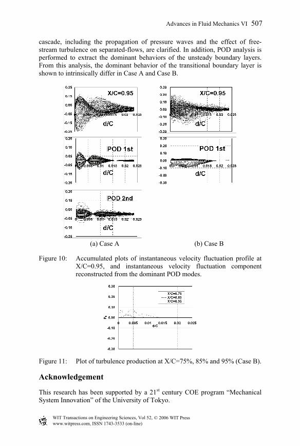
In Case A, pressure waves that originate from the unsteady fluctuation in the neighborhood of the trailing-edge propagate in almost entire region of the blade passage. The pressure waves oscillate the separation bubble that is formed near 80% chord length position. Also they reach the suction side of the neighboring blade at its maximum curvature and form a complex pressure field upstream of the blade’s throat. In the boundary layer near the trailing-edge, spanwise vorticies are created due to the boundary layer separation and they are convected downstream while maintaining the periodic variation of the wakes near the trailing-edge. To the contrary, no strong periodic pressure waves are generated from the neighborhood of the trailing-edge in Case B. After the generation of turbulent spots, fully three-dimensional turbulent boundary layer convects downstream and the wake consists of minute three-dimensional eddies. In order to extract dominant unsteady behaviors of the transitional boundary layer, POD Analysis is performed. The method used in the present study is Sirovich’s Snapshot POD Method [7]. Figure 10 shows accumulated plots of instantaneous velocity fluctuation profile at X/C=0.95, and instantaneous velocity fluctuation component reconstructed from the dominant POD modes for both Case A and Case B. In Case A, the sign of the 2nd mode changes at a point further apart from the wall than the 1st mode. In fig. 8, the vorticies near the trailing-edge are compressed and expanded by the passage of pressure waves as is found in the relationship between the divergence value and the vortices. Therefore, the difference in the position where the sign changes in the 1st mode and the 2nd mode corresponds to the compression and expansion of the vorticies. Furthermore, the region swept by the profiles of the 2nd mode has asymmetry regarding the abscissa. This asymmetry corresponds to the deformation of the spanwise vorticies in the spanwise direction near the trailing-edge as is found in fig. 8. Based on the above discussion, in addition to the passage of the pressure waves, the compression and expansion of the vorticies due to the passage of the pressure waves are the dominant behavior of the boundary layer in the no free-stream turbulence case. Especially at 95% chord length position, the spanwise deformation of vortices is also the dominant unsteady behavior of the transitional boundary layer. On the other hand, as is found in the similarity of the shape of the region swept by the 1st mode to the turbulence production at X/C=0.95, the dominant behavior of the transitional boundary layer is the turbulence production in Case B. Therefore, the dominant behavior of the transitional boundary layer is intrinsically different in Case A and Case B.

5 Conclusions

Large eddy simulation of compressible transitional flows in a low-pressure turbine cascade is performed by using 6th-order compact difference and 10th-order filtering method. Numerical results without free-stream turbulence and those with approximately of 5% free-stream turbulence are compared. Based on the computed results, differences in the unsteady behaviors of flows in the



cascade, including the propagation of pressure waves and the effect of free-stream turbulence on separated-flows, are clarified. In addition, POD analysis is performed to extract the dominant behaviors of the unsteady boundary layers. From this analysis, the dominant behavior of the transitional boundary layer is shown to intrinsically differ in Case A and Case B.

(a) Case A (b) Case B

Figure 10: Accumulated plots of instantaneous velocity fluctuation profile at X/C=0.95, and instantaneous velocity fluctuation component reconstructed from the dominant POD modes.

Figure 11:

This research has been supported by a 21st century COE program “Mechanical System Innovation” of the University of Tokyo.

Plot of turbulence production at X/C=75%, 85% and 95% (Case B).

Acknowledgement



The authors would also like to thank an IT research program “Frontier Simulation Software for Industrial Science” supported by the Ministry of Education, Culture, Sports, Science and Technology (MEXT), and a collaborative research project with Japan Aerospace Exploration Agency (JAXA) “Simulation of Internal Flows in Rocket Engines,” both of which provided computational resources needed to pursue this research.

References

[1] Mayle, R.E., The role of laminar-turbulent transition in gas turbine engines. Trans. ASME, Journal of Turbomachinery, 113, pp. 509-537, 1991.

[2] Emmons, H.W., The laminar-turbulent transition in a boundary layer-part I. Journal of the Aeronautical Sciences, 18, pp. 490-498, 1951.

[3] Raverdy, B., Mary, I. & Sagaut, P., High-resolution large-eddy simulation of flow around low-pressure turbine blade. AIAA Journal, 41(3), pp. 390-397, 2003.

[4] Wu, X. & Durbin, P.A., Evidence of longitudinal vortices evolved from distorted wakes in a turbine passage. Journal of Fluid Mechanics, 446, pp. 199-228, 2001.

[5] Michelassi, V., Wissink, J.G., Fröhlich, J. & Rodi, W., Large-eddy simulation of flow around low-pressure turbine blade with incoming wakes. AIAA Journal, 41(11), pp. 2143-2156, 2003.

[6] Matsuura, K., Large eddy simulation of compressible transitional cascade flows. Transactions of the Japan Society of Mechanical Engineers, 70(700), B, pp. 3066-3073, 2004 (in Japanese).

[7] Sirovich, L. & Rodriguez, J.D., Coherent structures and chaos: a model problem. Physics Letters A, 120(5), pp. 211-214, 1987.

[8] Lele, S.K., Compact finite difference schemes with spectral-like resolution. Journal of Computational Physics, 103, pp. 16-42, 1992.

[9] Gaitonde, D.V. & Visbal, M.R., Padé-type higher-order boundary filters for the Navier-Stokes equations. AIAA Journal, 38(11), pp. 2103-2112, 2000.

[10] Voke, P., Subgrid-scale modelling at low mesh Reynolds number. Theoretical and Computational Fluid Dynamics, 8, pp. 131-143, (1996).

[11] Pironneau, O., Rodi, W., Ryhming, I.L., Savill, A.M. & Truong, T.V., Numerical simulation of unsteady flows and transition to turbulence. Proceedings of the ERCOFTAC Workshop held at EPFL 26-28 March 1990 Lausanne, Switzerland, Cambridge University Press, (1990).

[12] Fottner, L., (ed). Test Cases for Computation of Internal Flows in Aero Engine Components. AR-275, AGARD, pp. 112-123, 1990.



large eddy simulation of compressible transitional cascade ... · keywords: large eddy simulation,...

Documents