large area scene selection interface (lassi) … · limitations that the landsat satellites have:...

Pecora 17 – The Future of Land Imaging…Going Operational November 18 – 20, 2008 ♦ Denver, Colorado

LARGE AREA SCENE SELECTION INTERFACE (LASSI) METHODOLOGY OF SELECTING LANDSAT IMAGERY FOR THE GLOBAL LAND

SURVEY 2005

Shannon Franks, Faculty Research Assistant University of Maryland

Department of Geography College Park, MD 20742

[email protected]

Rachel M. K. Headley, Data Acquisition Manager, Acting USGS EROS

Sioux Falls, SD 57198 [email protected]

ABSTRACT The Global Land Survey (GLS) 2005 is a cloud-free, orthorectified collection of Landsat imagery acquired during the 2004-2007 epoch designed to support global land-cover and ecological monitoring. Due to the numerous complexities in selecting imagery for the GLS2005, NASA and the U.S. Geological Survey (USGS) sponsored the creation of an automated scene selection tool, the Large Area Scene Selection Interface (LASSI), to select the scenes for inclusion in this data set. This innovative approach to scene selection applied a user-defined weighting system to various scene parameters: image cloud cover, image vegetation greenness, choice of sensor, and the ability of the Landsat 7 scan line corrector (SLC)-off pair to completely fill image gaps, amongst others. The parameters considered in scene selection were weighted according to their relative importance to the data set, along with the algorithm’s sensitivity to that weight. Although using LASSI was a significant advancement over selecting images manually, in certain circumstances it was necessary for human inspection and correction. Furthermore, there were numerous challenges that were faced along the scene selection process that led to many lessons learned that resulted in a change to the base algorithm. This paper describes the methodology and analysis that determined the parameter weighting strategy and post-screening processes used in selecting the optimal data set for GLS2005.

INTRODUCTION Monitoring global changes in land cover remains a priority for remote sensing science. In order to produce

reliable measures of land-cover change and disturbance, researchers require a baseline set of cloud-free, leaf-on imagery. The Global Land Survey (GLS – formerly known as “Geocover”) data sets provide wall-to-wall, cloud-free Landsat coverage of the Earth’s land areas for epochs centered on 1975, 1990, 2000, and 2005. These data sets provide the science and conservation communities a comprehensive view of how the planet’s land areas have changed over the last thirty-five years.

The goal of the Global Land Survey 2005∗ (GLS2005) was to provide one clear image during leaf-on conditions for every location of the global land area during the 2004-2007 period (Gutman et al., 2008). In total, approximately 9,500 Landsat images was included in GLS2005 data set, an increase compared to the 1990 GeoCoverTM (~7,000 scenes) and the 2000 GeoCoverTM (~8,200 scenes). This increase reflects additional coastal and island areas not represented in the earlier GeoCoverTM initiatives and the inclusion of the Landsat Image Mosaic of Antarctica (LIMA), to support the International Polar Year. The GLS2005 was a cooperative activity between NASA and USGS with science steering group members being constituents from NASA headquarters, NASA Goddard Space Flight Center, USGS headquarters, USGS EROS, University of Maryland, Aerospace Corporation, Lockheed Martin, and Emalico LLC.

∗ The GeoCover™ 2000 data set has been reprocessed to improve the geometric accuracy and establish a

control baseline for GLS2005, the other GeoCover™ data sets, and current Landsat product generation. After reprocessing, the GeoCover™ data sets are renamed GLS.


Akin to creating any “best of” data set, selecting imagery poses a formidable challenge. Not only do the user’s desires not always align, but the increasing number of moderate-resolution remote sensing systems provides a wide array of available data sets. The primary use of the GLS data sets are to monitor land use and land cover changes at a moderate-resolution scale. In an attempt to remain consistent with the previous GLS data sets, the GLS science steering group decided upon using as much Landsat data as was possible. Landsat 5 and Landsat 7 data would be used for the majority of the globe, but also Earth Observing 1’s Advanced Land Imager (EO-1 ALI) imagery and Terra Advanced Spaceborne Thermal Emission and Reflection Radiometer (ASTER) data as needed. This not only reflects the diversity of Landsat-like resolution remote sensing satellites in orbit, but also highlights the major limitations that the Landsat satellites have: the inability to secure global coverage with Landsat 5 Thematic Mapper (TM), and the failure of the Landsat 7 Enhanced Thematic Mapper Plus (ETM+) Scan Line Corrector (SLC) in 2003 (Gutman et al., 2008).

This paper describes the process of scene selection for the GLS2005 data set. In order to automate scene selection the GLS project, in collaboration with NASA Ames Research Center, developed a new tool to generate optimal collections of imagery using metadata statistics and user-defined weighting criteria. In the sections below, we describe the parameters used in scene selection, discuss the reasoning behind the weighting of those parameters, talk briefly about the post screening processes, show the results of the scene selection of North America, and reveal the lessons that where learned along the way.

BACKGROUND There are three existing global survey data sets: GeoCover™ 1975, 1990, and 2000. These were produced by

the EarthSat Corporation (now MDA Federal, Inc.) under contract to NASA. Scene selection for these data sets was based on visual aspects of the imagery, like clouds, haze, missing scan lines, and other manifestations of poor data quality. Image characteristics were weighed against the year and season in which the data were acquired (Tucker et al., 2004). While scene selection was labor intensive, it was feasible because only a few characteristics were considered, and most of them were assessed quickly by visual inspection. For GLS2005, not only were there more data available, but the task became considerably more complicated due to the failure of the Landsat 7 ETM+ SLC in 2003 (Williams et al., 2006).

Landsat 7 continues to acquire global coverage, but with the SLC failure each scene is missing approximately 22 percent of its area coverage in cross-track, bow-tie shapes starting from each edge. The most suitable workaround for these missing data in ETM+ scenes is to “gap fill” the imagery with other imagery from the same growing season. Although this is a credible strategy (Masek, 2007), it makes scene selection more complex. It was necessary to not only select the best base scene for that Worldwide Reference System (WRS) path and row, but also the best associated fill scene. Occasionally, two fill scenes were chosen to gain better geographic coverage of the scene.

The added complexities of dealing with gap-filled imagery did raise the question of whether Landsat 7 ETM+ data should be used for the dataset. The GLS2005 science steering group and user community representatives decided that, in situations where the “base” and “fill” scenes were cloud-free and the land cover was not a seasonally dynamic land cover type such as agriculture, it was preferable to use Landsat 7 “gap-filled” imagery due to its superior geometry and radiometry when compared to Landsat 5 TM.

GLS2005 primarily consists of Landsat 5 TM and Landsat 7 ETM+ imagery where possible, but it was also supplemented by ALI and ASTER data. Given the smaller swath-width of the ALI instrument (30km), the primary application was obtaining images of small islands and reefs. ASTER imagery was used to fill in some problematic regions (eg. Northern Eurasia) where no suitable Landsat data were available.

LARGE AREA SCENE SELECTION INTERFACE TOOL Some 400,000 Landsat images were considered in scene selection by the LASSI tool for GLS2005. These were

reduced to fill 9,500 Worldwide Reference System (WRS) locations based on several criteria that included acquisition date, cloud cover, gap-fill coverage, sensor choice, and geographic uniformity, amongst others. To handle the large number of scenes in the selection pool, and the increased complexities in scene selection for GLS2005, NASA Goddard Space Flight Center (GSFC) and USGS Earth Resources Observation and Science Center (EROS) sponsored the creation of an automated scene selection tool. This tool, called LASSI, was


developed by NASA Ames Research Center. The LASSI applies non-linear optimization to identify the “best” selection of scenes from a user-defined weighting system to pre-determined scene parameters. With supplied metadata, LASSI can quickly and systematically sort through thousands of scenes to select the best overall set to make an area solution. For the sake of simplicity, this paper describes the methods used in determining the weighting only for the North American continent. For details about the weighting scheme used for the other continents, please contact the authors directly. For more information on the algorithmic basis for the tool, see Khatib et al. (2007).

Selection Parameters

Description. During scene selection, there were 14 parameters considered by LASSI. Each parameter was given a weighting by the LASSI operator to reflect its importance for scene selection for a particular region. These factors and their associated weightings drove the scene selection. All Landsat 7 imagery required image pairs to provide complete coverage. An L7 “base” scene is the scene that covers 78 percent of the image area. The L7 “fill” image fills some or all of the remaining 22 percent gap. Fill image parameters apply only to Landsat 7.

• NDVI- base Image: Climatological NDVI of Landsat 5 (L5) image or Landsat 7 (L7) base image, interpolated from a mean monthly NDVI record. For this factor, the Pathfinder (PALS) AVHRR NDVI time series was used after sub-averaging 8km resolution monthly values to the area of each WRS-2 path/row (James and Kalluri, 1994).

• NDVI- fill Image: NDVI of the L7 fill image. • ACCA- base Image: The Automated Cloud Cover Assessment (ACCA) score is generated during L7

image processing and reports the percentage of clouds present in the L7 imagery at a precision of 1% cloud cover. The cloud score algorithm for L5 results in a coarser estimate (10% cloud cover increments). For GLS2005, all L5 imagery was manually prescreened to only include cloud-free scenes. Increasing this weight favored clear scenes for L7 base imagery or clear L5 images.

• ACCA- fill Image: ACCA score for L7 fill image. • Difference in Acquisition Dates between L7 gap-filled pairs: Increasing this parameter favored L7 base/fill

pairs with minimal seasonal difference between them, and resulted in favoring L5 imagery (which was considered to have zero difference). This factor became important for areas where vegetation changed rapidly—over agricultural fields or in areas that have a short growing season, for example.

• Difference in Acquisition Dates between L7 gap-filled pairs (over agriculture): This parameter worked in conjunction with the previous one, but only had effect when agriculture was present, as defined by the MODIS landcover product, MOD12 (LPDAAC, 2001). In essence, it added weighting to the parameter “Difference in acquisition dates between L7 gap-filled pairs”, scaled to the percent of the WRS that is agriculture. An example of how this parameter works can be found in the section detailing parameter weighting.

• Area coverage: This factor influenced how much of the scene area was covered by Landsat imagery. For L5, coverage will always be 100 percent of the scene area. For L7, if only one image is used, 78 percent of the area is covered. Where L7 pairs are used, the area coverage can vary between 78% and 100%. Increasing this factor drove LASSI to select L7 image pairs that achieved as close to 100 percent coverage as possible, or to select an L5 image. It is important to note that increasing this parameter weight did not specifically prefer L7 data, but preferenced high area coverage for that WRS, regardless of sensor choice.

• Difference in Day of Year between North-South neighbors: This parameter weighted the importance of close dates of acquisition (irrespective of year) between the North-South neighbors. By optimizing this factor, the seasonality was minimized in the north-south direction.

• Difference in Day of Year between East-West neighbors: This parameter weighted the importance of close dates of acquisition (irrespective of year) between the East-West neighbors. By optimizing this factor, the seasonality was minimized in the East-West direction.

• Preference Landsat 5 Imagery: Increasing this parameter favored LASSI selection of L5 imagery. • Preference Landsat 7 Imagery: Increasing this parameter favored LASSI selection of L7 imagery. • Sensor Homogeneity: Increasing this parameter favored contiguous spatial groups of a single sensor (L5 or

L7). It is this parameter, along with the Difference in Day of Year between the North-South and East-West neighbors, which provided uniformity of the data set.

• Preference towards a Specific Date Range: For GLS2005, there was a desire to select scenes that were acquired during the middle of the decade (2005 and 2006) as opposed to 2004 and 2007. Increasing the weighting of this parameter influenced that decision.


• Preference Day of Year: This parameter puts a preference towards selecting scenes from the same time of year as the GeocoverTM 2000 data set. This optimizes data to facilitate change-over-time research between the two datasets.

Parameter Weighting (with Metadata Visualizations)

For the North American continent, the weighting values in Table 1 were used to select the data set. The scene selection for other continents had a slightly different weighting scheme to adapt to the differing characteristics of those regions. The numerical values are unitless and simply express the relative weights assigned to various data set characteristics (explained below).

Table 1. Parameter weightings used for North America scene selection for GLS2005.

Parameter Value Description NDVI_B 60 NDVI – base image NDVI_F 30 NDVI – fill image ACCA_B 20 ACCA – base image ACCA_F 20 ACCA – fill image difAD_P 10 Difference in acquisition dates between L7 gap-filled pairs difAD_P (ag) 40 Diff. in acquisition dates between L7 gap-filled pairs (over agriculture) Coverage_P 15 Area coverage difDY_NS 4 Diff. in day of year between N-S neighbors difDY_EW 4 Diff. in day of year between E-W neighbors L5_pref 0 Preference L5 imagery L7_pref 10 Preference L7 imagery SensHomg 5 Sensor homogeneity Date_pref 10 Preference towards a specific date range (2005 and 2006) DOY_pref 15 Preference day of year (Geocover 2000TM)

NDVI - base and fill Images. Maximizing the NDVI of the base and fill images was given the greatest weight, since imagery at the peak of the growing season is critical for land cover and land use change analysis, the principal use of the GLS data sets. In Figure 1, the NDVI values have been scaled to represent the percent of maximum NDVI for each scene (WRS locations will be referred to hereafter as "scenes"). By displaying the map as percent of maximum, it can easily be determined if the parameter was successfully optimized. Normalizing the values allowed comparable analysis of scenes with a low NDVI average (e.g., deserts) and scenes of high average NDVI. The fill image was also strongly weighted, to minimize the differences between the NDVI values of the Landsat 7 gap-filled image pairs (Figure 2). This also ensured that both images were acquired within the growing season. The average absolute NDVI for the base (Landsat 7 and Landsat 5) images was 0.560.


Figure 1. NDVI of base imagery. The values here are percent of maximum NDVI for each WRS.

Figure 2. Difference of NDVI between Landsat 7 image pairs. Landsat 5 images have a difference NDVI of 0.

ACCA- base and fill Images. The ACCA for the base and fill images was not heavily weighted because the input images were initially filtered such that LASSI was selecting from imagery with 10 percent or less cloud cover. Previous research showed that gap-filling of Landsat 7 imagery only worked well when both the base and fill images are cloud-free (Masek, 2007). In cases when either the base or fill image had clouds, the histogram matching between the images resulted in the cloud radiometry contaminating the pixels of the accompanying image. This research led to the requirement that the base image be restricted to 4 percent or less cloud cover and the corresponding fill image to 8 percent or less. If either of those requirements was exceeded and no alternative was


available, the base and fill images were left as single images in the final data set rather than being processed as a gap-filled pair. The average cloud cover of the data set was extremely low, with less than 1 percent clouds (0.757 ACCA) in the base imagery (Figure 3) and a 1.7 ACCA in the fill imagery.

Figure 3. ACCA scores for Landsat base images.

Difference in Acquisition Dates between Landsat 7 gap-filled pairs. In most cases, the difference in acquisition dates between Landsat 7 gap-filled pairs was not as important as the difference of NDVI in Landsat 7 pairs. If the difference of NDVI parameters between base and fill (NDVI_B, NDVI_F) were properly weighted, the temporal difference between base and fill images would be minimized. For that reason, this parameter (difAD_P) was weighted lower with a value of 10. However, in regions of rapid changes, such as croplands, the temporal difference was not sufficiently minimized using NDVI alone. For these regions, scenes acquired several cycles apart were not acceptable due to the resulting phenological differences. As a result, a second parameter specific to agricultural scene content (difAD_P(ag)) was created to adjust the weighting applied to the original difAD_P parameter, as a function of the percentage of cropland in each scene. After some trial runs, a value of 40 was assigned to the new parameter. Over most of the globe, where there is not classifiable agriculture, the difAD_P (ag) parameter had no impact, as shown in equation (1) below. But in parts of the world where there is agriculture, the factor became relevant. For example, if a certain WRS is defined (by MODIS land cover product, MOD12) as 80 percent croplands, the total addition of the two difAD_P parameters would be 42, as shown in equation (2). See Figure 4 for the temporal difference between Landsat 7 pairs in the North America selected data set.

(1) 10 + 0.0(40) = 10 (2) 10 + 0.8(40) = 42


Figure 4. Temporal difference between Landsat 7 pairs (Landsat 5 scenes have a value of 0, since the data is not gap filled with another image). The small temporal difference in the croplands belt is the result of the agricultural

parameter. Overall, the average temporal difference between the Landsat 7 pairs was 39 days.

Area Coverage. The goal for GLS2005 was to have at least 95 percent of each Landsat 7 scene covered between the base and fill scenes (Figure 5). Complete area coverage was easy to achieve in areas with many available candidate scenes, but was more of a challenge where candidates were more limited. To attain adequate coverage, on rare occasions it was necessary to add a second fill scene. Area coverage was most often at odds with the difference in NDVI, where the best NDVI match did not always fulfill the area coverage requirement. In these situations, the decision was made to include the two images that were seasonally consistent and try to again supplement the outstanding area coverage with the addition of a second fill scene.


Figure 5. Scene area coverage for each WRS. Average gap-fill for the Landsat 7 pairs was 95.5 percent. Landsat 5

data has 100 percent area coverage. The average area coverage of the continent was 97.2 percent.

Difference in Day of Year for East-West and North-South Neighbors. The Difference in Day of Year for East-West and North-South Neighbors parameters were useful to minimize the seasonality differences between neighboring paths or rows, but not as important to data set quality as some of the other parameters. The North-South effect was not satellite-specific. However, the East-West effect could result in one path consisting mainly of Landsat 5 imagery and the next path consisting mainly of Landsat 7 data, due to the 8-day difference between the two satellites as compared to the standard 16-day satellite revisit cycle of each individual satellite.

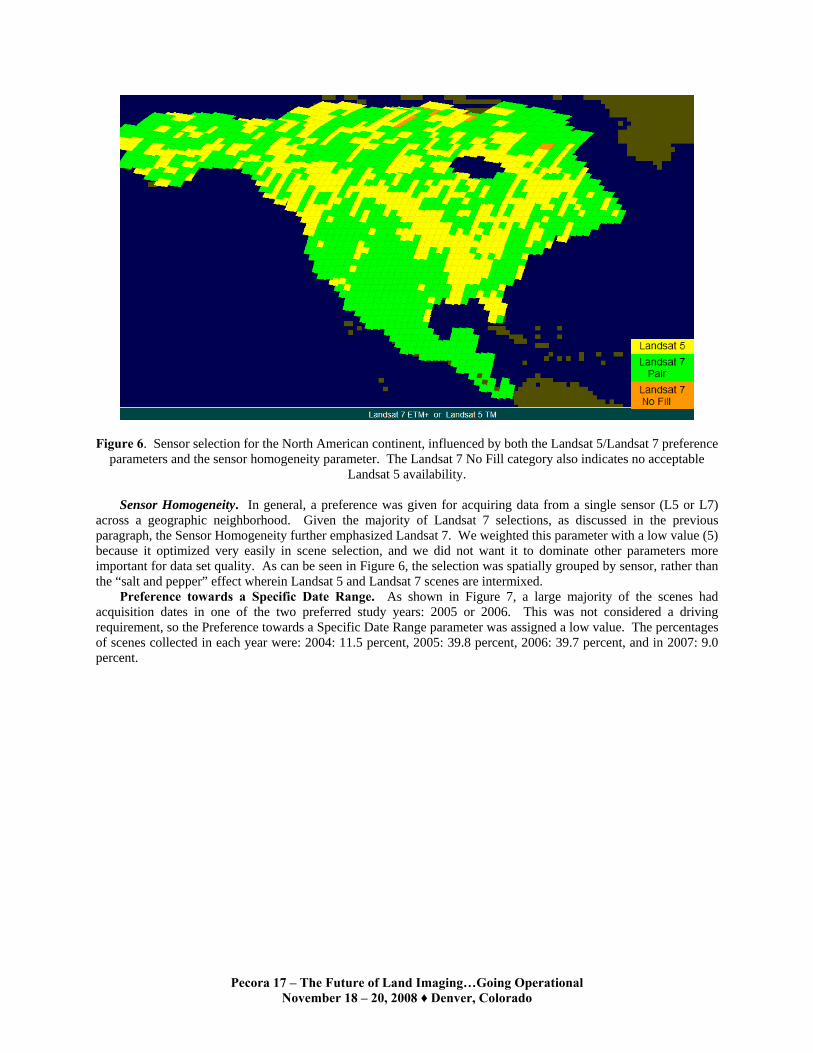
Sensor Preference. Landsat 7’s superior radiometric and geometric properties led to a slight preference for using Landsat 7 imagery over Landsat 5 imagery, although in many areas outside of the U.S. Landsat Ground Station, the available archive from either sensor was limited. For North America, we weighted only the Landsat 7 parameter, at a low value of 10, so that it became a “tie-breaker” when LASSI had both a suitable Landsat 7 image pair and a suitable Landsat 5 scene for the same WRS. As seen in Figure 6, LASSI predominantly selected Landsat 7 imagery (63 percent) except in the agriculture belt of the United States, where the temporal difference between the Landsat 7 base and fill images was often unacceptable.


Figure 6. Sensor selection for the North American continent, influenced by both the Landsat 5/Landsat 7 preference

parameters and the sensor homogeneity parameter. The Landsat 7 No Fill category also indicates no acceptable Landsat 5 availability.

Sensor Homogeneity. In general, a preference was given for acquiring data from a single sensor (L5 or L7)

across a geographic neighborhood. Given the majority of Landsat 7 selections, as discussed in the previous paragraph, the Sensor Homogeneity further emphasized Landsat 7. We weighted this parameter with a low value (5) because it optimized very easily in scene selection, and we did not want it to dominate other parameters more important for data set quality. As can be seen in Figure 6, the selection was spatially grouped by sensor, rather than the “salt and pepper” effect wherein Landsat 5 and Landsat 7 scenes are intermixed.

Preference towards a Specific Date Range. As shown in Figure 7, a large majority of the scenes had acquisition dates in one of the two preferred study years: 2005 or 2006. This was not considered a driving requirement, so the Preference towards a Specific Date Range parameter was assigned a low value. The percentages of scenes collected in each year were: 2004: 11.5 percent, 2005: 39.8 percent, 2006: 39.7 percent, and in 2007: 9.0 percent.


Figure 7. The distribution of scenes that were acquired within the preferred years (2005 and 2006) of the survey period.

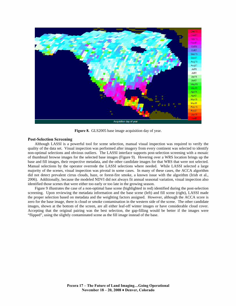
Preference Day of Year. This factor put a preference on selecting scenes that were close in date to the GeocoverTM 2000 data set. For land-cover and land-use change (LCLUC) analysis, matching acquisition days of year would facilitate studies using the GeoCoverTM 2000 and GLS2005 data sets. However, the time of year selected for the GeocoverTM 2000 images was not always optimal, with many scenes being late in the growing season to avoid cloud cover (Tucker et al., 2004). In weighting this parameter for GLS2005, there was a balance between selecting scenes that were temporally close to those of the GeocoverTM 2000 data set, and avoiding the possible degradation of the quality of the data set by doing so. Our analysis showed that a weight of 15 would accomplish this goal. The GLS2005 selected day of year are shown in Figure 8. These results demonstrate the correction of the seasonality selection errors of the GeoCoverTM 2000 data set.


Figure 8. GLS2005 base image acquisition day of year.

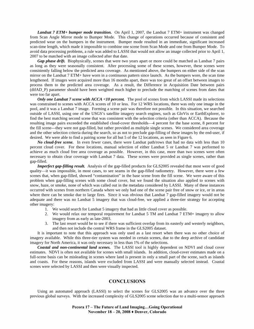
Post-Selection Screening Although LASSI is a powerful tool for scene selection, manual visual inspection was required to verify the

quality of the data set. Visual inspection was performed after imagery from every continent was selected to identify non-optimal selections and obvious outliers. The LASSI interface supports post-selection screening with a mosaic of thumbnail browse images for the selected base images (Figure 9). Hovering over a WRS location brings up the base and fill images, their respective metadata, and the other candidate images for that WRS that were not selected. Manual selections by the operator overrode the LASSI selections where needed. While LASSI selected a large majority of the scenes, visual inspection was pivotal in some cases. In many of these cases, the ACCA algorithm did not detect prevalent cirrus clouds, haze, or forest-fire smoke, a known issue with the algorithm (Irish et al., 2006). Additionally, because the modeled NDVI did not always fit annual seasonal variation, visual inspection also identified those scenes that were either too early or too late in the growing season.

Figure 9 illustrates the case of a non-optimal base scene (highlighted in red) identified during the post-selection screening. Upon reviewing the metadata information and the base scene (left) and fill scene (right), LASSI made the proper selection based on metadata and the weighting factors assigned. However, although the ACCA score is zero for the base image, there is cloud or smoke contamination in the western side of the scene. The other candidate images, shown at the bottom of the screen, are all either leaf-off winter images or have considerable cloud cover. Accepting that the original pairing was the best selection, the gap-filling would be better if the images were “flipped”, using the slightly contaminated scene as the fill image instead of the base.


Figure 9. LASSI post-screening interface showing an example of non-optimal base-fill assignment, where “flipping” the LASSI assignments would result in a better gap-filled product.

At times, the operator was required to make a choice between two very similar images. If the modeled NDVI

(based on the date of acquisition) of both scenes was similar, then the images were visually analyzed to determine which one was in a higher stage of seasonal green-up. If, after that examination, the decision was still not clear, the inspector would select the one that was later in the season, especially in the northern regions of Canada and Alaska where the growing season has a slow start due to ice melt-off in the spring.

Special Cases and Exceptions

Processing Landsat 7 scenes pairs is very common – almost 40 percent of all recent Landsat 7 sales use multiple scenes. However, the processing of over 9,000 scenes for GLS2005 has given an unprecedented view into the nuances of scene selection for SLC-off image pairs. In addition, areas of consistent clouds during the growing season proved extremely difficult to select, even with the depth of the U.S. archive. Selecting scenes for the North American continent provided many lessons learned. The following special cases and exemptions were identified during the selection and subsequent screening processes.

Scene Information


Landsat 7 ETM+ bumper mode transition. On April 1, 2007, the Landsat 7 ETM+ instrument was changed from Scan Angle Mirror mode to Bumper Mode. This change of operations occurred because of consistent and predicted wear on the bumpers in the instrument. Bumper mode resulted in an immediate, significant increased scan-time length, which made it impossible to combine one scene from Scan Mode and one from Bumper Mode. To avoid data processing problems, a rule was added to LASSI that would not allow an image collected prior to April 1, 2007 to be matched with an image collected after that date.

Gap phase drift. Biophysically, scenes that were two years apart or more could be matched as Landsat 7 pairs as long as they were seasonally consistent. After processing some of these scenes, however, these scenes were consistently falling below the predicted area coverage. As mentioned above, the bumpers on either side of the scan mirror on the Landsat 7 ETM+ have worn in a continuous pattern since launch. As the bumpers wore, the scan time lengthened. If images were acquired more than 16 months apart, there was too great of an offset between images to process them to the predicted area coverage. As a result, the Difference in Acquisition Date between pairs (difAD_P) parameter should have been weighted much higher to preclude the matching of scenes from dates that were too far apart.

Only one Landsat 7 scene with ACCA <10 percent. The pool of scenes from which LASSI made its selections was constrained to scenes with ACCA scores of 10 or less. For 12 WRS locations, there was only one image in the pool, and it was a Landsat 7 image. Forming a scene pair was therefore not possible. In this situation, we searched outside of LASSI, using one of the USGS’s satellite imagery search engines, such as GloVis or EarthExplorer, to find the best matching second scene that was consistent with the selection criteria (other than ACCA). Because the resulting image pairs exceeded the established cloud-cover thresholds—4 percent for the base scene, 8 percent for the fill scene—they were not gap-filled, but rather provided as multiple single scenes. We considered area coverage and the other selection criteria during the search, so as not to preclude gap-filling of these images by the end-user, if desired. We were able to find a pairing scene for all but 5 of the 12 locations, as seen in Figure 6.

No cloud-free scene. In even fewer cases, there were Landsat path/rows that had no data with less than 10 percent cloud cover. For these locations, manual selection of either Landsat 5 or Landsat 7 was performed to achieve as much cloud free area coverage as possible. However, in this case, more than two scenes were often necessary to obtain clear coverage with Landsat 7 data. These scenes were provided as single scenes, rather than gap-filled.

Imperfect gap-filling result. Analysis of the gap-filled products for GLS2005 revealed that most were of good quality—it was impossible, in most cases, to see seams in the gap-filled radiometry. However, there were a few scenes that, when gap-filled, showed “contamination” in the base scene from the fill scene. We were aware of this problem when gap-filling scenes with some cloud cover, but we found the situation also applied to scenes with snow, haze, or smoke, none of which was called out in the metadata considered by LASSI. Many of these instances occurred with scenes from northern Canada where we only had one of the scene pair free of snow or ice, or in areas where there can be smoke due to large fires. Since it was obvious that Landsat 7 gap-filled imagery would not be adequate and there was no Landsat 5 imagery that was cloud-free, we applied a three-tier strategy for accepting other imagery:

1. We would search for Landsat 5 imagery that had as little cloud cover as possible. 2. We would relax our temporal requirement for Landsat 5 TM and Landsat 7 ETM+ imagery to allow

imagery from as early as late-2003. 3. The last resort would be to see if there was sufficient overlap from its easterly and westerly neighbors,

and then not include the central WRS frame in the GLS2005 dataset. It is important to note that this approach was only used as a last resort when there was no other choice of

imagery available. While this three-tier system was needed in certain scenes, due to the deep archive of candidate imagery for North America, it was only necessary in less than 1% of the selections.

Coastal and non-continental land scenes. The LASSI tool is highly dependent on NDVI and cloud cover estimates. NDVI is often not available for scenes with small islands. In addition, cloud-cover estimates made on a full-scene basis can be misleading in scenes where land is present in only a small part of the scene, such as islands and coasts. For these reasons, islands were excluded from LASSI and were manually selected instead. Coastal scenes were selected by LASSI and then were visually inspected.

CONCLUSIONS Using an automated approach (LASSI) to select the scenes for GLS2005 was an advance over the three

previous global surveys. With the increased complexity of GLS2005 scene selection due to a multi-sensor approach


and issues associated with gap-filled data, scene selection without the use of a computer algorithm would have been extremely labor intensive. Although using the LASSI tool dramatically eased this complex process, human input and guidance was still required to properly weight the parameters and review the results. Learning the tendencies of the algorithm in order to properly weight its selecting parameters was an effort within itself and took time to set the weighting scheme to obtain the “optimal” result for each continent or biome. There will be situations where users would prefer a different scene for their applications, but this is always a limitation of a single data set.

Overall, using LASSI has enabled us to select a data set that is superior to any other Global Land Survey. Previous GLS data sets were conceived as single-sensor data sets (e.g. MSS for GLS1975, Landsat 5 for GLS1990, and Landsat 7 for GLS2000). By expanding the available data sources to include both Landsat 5 and 7, as well as ASTER and EO-1, the GLS2005 had a richer selection of imagery to choose from. In addition, previous GLS data sets put a high priority on cloud-free coverage, but at the expense of obtaining leaf-on seasonality. Consequently, for some regions (e.g. dry deciduous tropics) the GLS1990 and GLS2000 data are not useful for mapping land cover conditions. By fine tuning the weighting criteria within LASSI we have more successfully balanced seasonality with cloud-clearing.

REFERENCES Gutman, G., R. Byrnes, J. Masek, S. Covington, S, C. Justice, S. Franks, and R. Headley, 2008. Towards monitoring

land cover and land-use changes at a global scale: The Global Land Survey 2005, Photogrammetric Engineering & Remote Sensing, 74(1).

Irish, R.R., J.L.Barker, S.N. Goward, and T. Arvidson, 2006. Characterization of the Landsat 7 ETM+ Automated Cloud-Cover Assessment (ACCA) Algorithm. Photogrammetric Engineering & Remote Sensing, 72(10): 1179-1188.

James, M. E. and S. N. V. Kalluri, 1994. The Pathfinder AVHRR land data set: An improved coarse resolution data set for terrestrial monitoring. International Journal of Remote Sensing, Special Issue on Global Data Sets. 15(17):3347-3363.

Khatib, L., J. Gasch, R. Morris, and S. Covington, Local Search for Optimal Global Map Generation Using Mid-Decadal Landsat Images, In Proceedings of AAAI Workshop on Preference Handling for Artificial Intelligence, Vancouver, BC, 2007.

LPDAAC, 2001. MODIS/Terra Land Cover Types Yearly L3 Global 0.05Deg CMG MOD12C1, URL: http://edcdaac.usgs.gov/modis/mod12c1v4.asp, U.S. Geological Survey (USGS) Center for Earth Resources Observation and Science (EROS), Sioux Falls, South Dakota (last date accessed: April 24, 2008).

Masek, J.G., 2007. White Paper on Use of Gap-Filled Products for the Mid-Decadal Global Land Survey (MDGLS), URL: http://lcluc.umd.edu/mdgls/documents/MDGLS_gapfill.pdf (last date accessed: April 14, 2008).

Tucker, C.J., D. Grant and J. Dykstra, 2004. NASA’s global orthorectified Landsat data set. Photogrammetric Engineering & Remote Sensing, 70: 313-322.

Williams, D.L., S. Goward, and T. Arvidson, 2006. Landsat: Yesterday, Today, and Tomorrow, Photogrammetric Engineering & Remote Sensing, 72 (10): 1171-1178.

large area scene selection interface (lassi) … · limitations that the landsat satellites have:...

Documents