laplace transform tutorial

8/7/2019 Laplace transform tutorial

http://slidepdf.com/reader/full/laplace-transform-tutorial 1/14

Tutorial 6

Laplace Transform

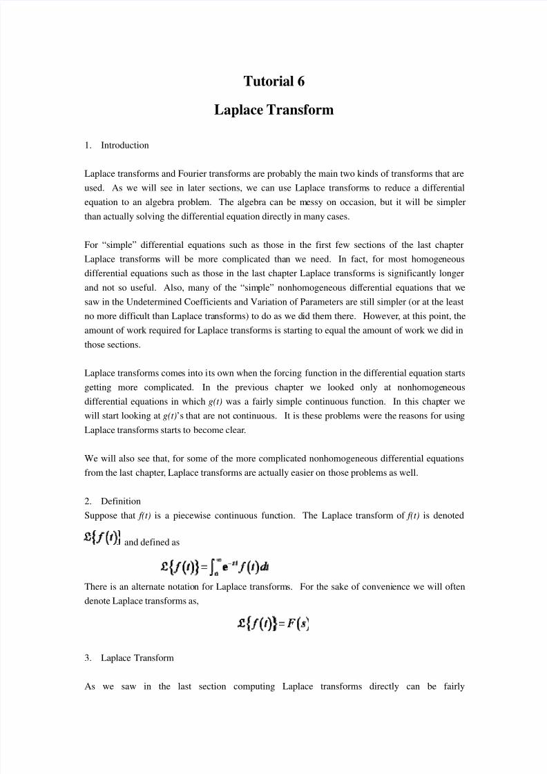
1. Introduction

Laplace transforms and Fourier transforms are probably the main two kinds of transforms that are

used. As we will see in later sections, we can use Laplace transforms to reduce a differential

equation to an algebra problem. The algebra can be messy on occasion, but it will be simpler

than actually solving the differential equation directly in many cases.

For “simple” differential equations such as those in the first few sections of the last chapter

Laplace transforms will be more complicated than we need. In fact, for most homogeneous

differential equations such as those in the last chapter Laplace transforms is significantly longer

and not so useful. Also, many of the “simple” nonhomogeneous differential equations that we

saw in the Undetermined Coefficients and Variation of Parameters are still simpler (or at the least

no more difficult than Laplace transforms) to do as we did them there. However, at this point, the

amount of work required for Laplace transforms is starting to equal the amount of work we did in

those sections.

Laplace transforms comes into its own when the forcing function in the differential equation starts

getting more complicated. In the previous chapter we looked only at nonhomogeneous

differential equations in which g(t) was a fairly simple continuous function. In this chapter we

will start looking at g(t)’s that are not continuous. It is these problems were the reasons for using

Laplace transforms starts to become clear.

We will also see that, for some of the more complicated nonhomogeneous differential equations

from the last chapter, Laplace transforms are actually easier on those problems as well.

2. Definition

Suppose that f(t) is a piecewise continuous function. The Laplace transform of f(t) is denoted

and defined as

There is an alternate notation for Laplace transforms. For the sake of convenience we will often

denote Laplace transforms as,

3. Laplace Transform

As we saw in the last section computing Laplace transforms directly can be fairly



complicated. Usually we just use a table of transforms when actually computing Laplace

transforms. The table that is provided here is not an inclusive table, but does include most of the

commonly used Laplace transforms and most of the commonly needed formulas pertaining to

Laplace transforms.



Example 1 Find the Laplace transforms of the given functions.

(a)



(b)

(c)

(d)

Solution

Okay, there’s not really a whole lot to do here other than go to the table, transform the individual

functions up, put any constants back in and then add or subtract the results.

(a)

(b)

(c)

(d)

Example 2 Find the transform of each of the following functions.

(a)

(b)

(c)

http://tutorial.math.lamar.edu/AllBrowsers/3401/Laplace_Table.asp

http://tutorial.math.lamar.edu/AllBrowsers/3401/Laplace_Table.asp



(d)

(e)

Solution

This function is not in the table of Laplace transforms. .

So, we then have,

we then have,

(b) We could use it with n=1.

Or we could use it with n=2.

Since it’s less work to do one derivative, let’s do it the first way.

The transform is then,

(c)

Now,

we get the following.

(d) For this part we’ll will use the answer from the previous part. To see this note that if



Then

Therefore, the transform is.

(e)

Remember that g(0) is just a constant so when we differentiate it we will get zero!

4. Inverse Laplace Transform

We are going to be given a transform, F(s), and ask what function (or functions) did we have

originally. As you will see this can be a more complicated and lengthy process than takingtransforms. In these cases we say that we are finding the Inverse Laplace Transform of F(s)

and use the following notation.

Example 3 Find the inverse transform of each of the following.

(a)



(b)

(c)

(d)

Solution

I’ve always felt that the key to doing inverse transforms is to look at the denominator and try to

identify what you’ve got based on that.

(a) From the denominator of the first term it looks like the first term is just a constant. The correct

numerator for this term is a “1” so we’ll just factor the 6 out before taking the inverse

transform. The second term appears to be an exponential with a = 8 and the numerator is exactly

what it needs to be. The third term also appears to be an exponential, only this time a = 3 and

we’ll need to factor the 4 out before taking the inverse transforms.

So, with a little more detail than we’ll usually put into these,

(b) The first term in this case looks like an exponential with a = -2 and we’ll need to factor out the

19. Be careful with negative signs in these problems, it’s very easy to lose track of them.

The second term almost looks like an exponential, except that it’s got a 3s instead of just an s in

the denominator. It is an exponential, but in this case we’ll need to factor a 3 out of the

denominator before taking the inverse transform.

The denominator of the third term appears to be in the table with n = 4. The numerator however,

is not correct for this. There is currently a 7 in the numerator and we need a 4! = 24 in the

numerator. This is very easy to fix. Whenever a numerator is off by a multiplicative constant, as

in this case, all we need to do is put the constant that we need in the numerator. We will just need

to remember to take it back out by dividing by the same constant.

So, let’s first rewrite the transform.



Let’s now take the inverse transform.

(c)

The transform becomes,

Taking the inverse transform gives,

(d)

Let’s do some slightly harder problems. These are a little more involved than the first set.

Example 4 Find the inverse transform of each of the following.

(a)

(b)

(c)

(d)



Solution

(a) From the denominator of this one it appears that it is either a sine or a cosine. However, the

numerator doesn’t match up to either of these in the table. A cosine wants just an s in the

numerator with at most a multiplicative constant, while a sine wants only a constant and no s in

the numerator. We’ve got both in the numerator. This is easy to fix however. We will just split

up the transform into two terms and then do inverse transforms.

Do not get too used to always getting the perfect squares in sines and cosines that we saw in the

first set of examples. More often that not they won’t be perfect squares!

(b) In this case there are no denominators in our table that look like this. We can however make the

denominator look like one of the denominators in the table by completing the square on the

denominator. So, let’s do that first.

Recall that in completing the square you take half the coefficient of the s, square this, and then add

and subtract the result to the polynomial. After doing this the first three terms should factor as a

perfect square.

So, the transform can be written as the following.

So, we will leave the transform as a single term and correct it as follows,



(c)

This one is similar to the last one. We just need to be careful with the completing the square

however. The first thing that we should do is factor a 2 out of the denominator, then complete the

square. Remember that when completing the square a coefficient of 1 on the s2 term is

needed! So, here’s the work for this transform.

In correcting the numerator of the second term, notice that I only put in the square root since we

already had the “over 2” part of the fraction that we needed in the numerator.

(d)

This one appears to be similar to the previous two, but it actually isn’t. The denominators in the

previous two couldn’t be easily factored. In this case the denominator does factor and so we need

to deal with it differently.

Here is the transform with the factored denominator.

The denominator of this transform seems to suggest that we’ve got a couple of exponentials,

however in order to be exponentials there can only be a single term in the denominator and no s’s

in the numerator.



To fix this we will need to do partial fractions on this transform. In this case the partial fraction

decomposition will be

Don’t remember how to do partial fractions? In this example we’ll show you one way of getting

the values of the constants and after this example we’ll review how to get the correct form of the

partial fraction decomposition.

Okay, so let’s get the constants. There is a method for finding the constants that will always

work, however it can lead to more work than is sometimes required. Eventually, we will need

that method, however in this case there is an easier way to find the constants.

Regardless of the method used, the first step is to actually add the two terms back up. This gives

the following.

Now, this needs to be true for any s that we should choose to put in. So, since the denominators

are the same we just need to get the numerators equal. Therefore, set the numerators equal.

Again, this must be true for ANY value of s that we want to put in. So, let’s take advantage of

that. If it must be true for any value of s then it must be true for , to pick a value at

random. In this case we get,

We found A by appropriately picking s. We can obtain B in the same way if we chose .

This will not always work, but when it does it will usually simplify the work considerably.

So, with these constants the transform becomes,

We can now easily do the inverse transform to get



5. Step Function

Before proceeding into solving differential equations we should take a look at one more

function. Without Laplace transforms it would be much more difficult to solve differential

equations that involve this function in g(t).

The function is the Heaviside function and is defined as,

Here is some alternate notation for Heaviside functions.

For Laplace transform, we get the following formula

Example 5

(a) Find the Laplace transform of

(b) Find the inverse Laplace transform of

Solution

(a) The first thing that we need to do is write the function in terms of step functions.

We had to add in a “-8” in the second term since that appears in the second part and we also had to

subtract a t in the second term since the t in the first portion is no longer there. This subtraction

of the t

adds a problem because the second function is no longer correctly shifted. This is easier to fix

than the

previous example however.

Here is the corrected function.



So, in the second term it looks like we are shifting

The transform is then,

(b) This one looks messier than it actually is. Let’s first rearrange the numerator a little.

In this form it looks like we can break this up into two pieces that will require partial

fractions. When we break these up we should always try and break things up into as few pieces

as possible for the partial fractioning. Doing this can save you a great deal of unnecessary

work. Breaking up the transform as suggested above gives,

Note that we canceled an s in F(s). You should always simplify as much a possible before doing

the partial fractions. Let’s partial fraction up F(s) first.

Setting numerators equal gives,

Now, pick values of s to find the constants.

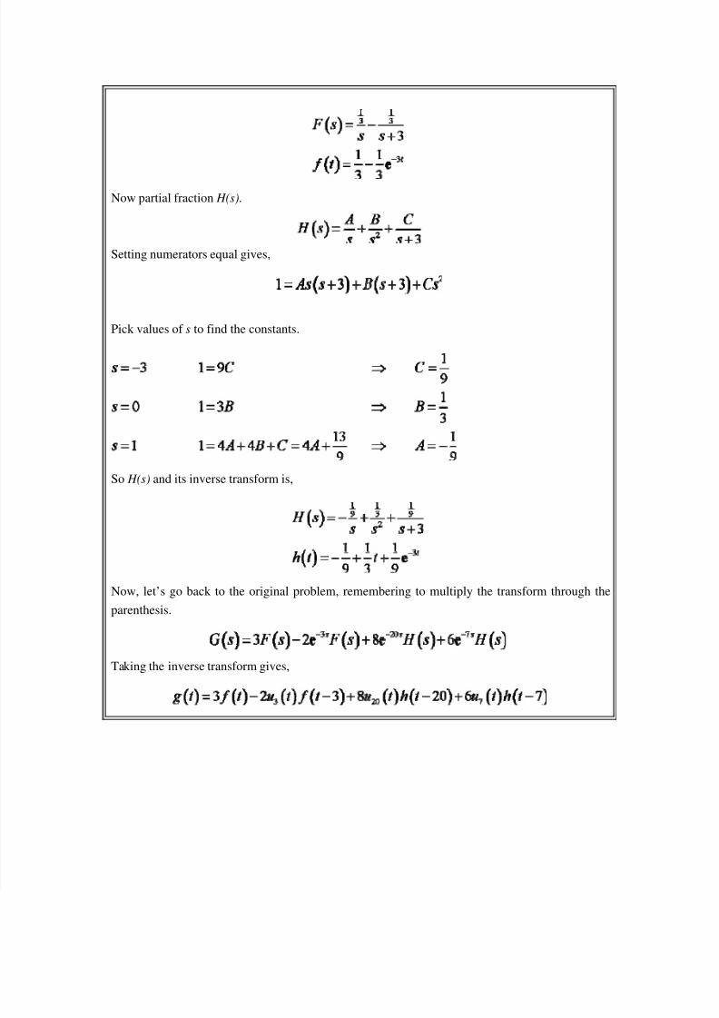
So F(s) and its inverse transform is,



Now partial fraction H(s).

Setting numerators equal gives,

Pick values of s to find the constants.

So H(s) and its inverse transform is,

Now, let’s go back to the original problem, remembering to multiply the transform through the

parenthesis.

Taking the inverse transform gives,

laplace transform tutorial

Documents