laplace transform (1/3) intro & differential...
TRANSCRIPT

Class Notes 12:
Laplace Transform (1/3)
Intro & Differential Equations
82 – Engineering Mathematics
Laplace Transform – Introduction

Laplace Transform – Introduction

Pierre Simon Laplace (Marquis)
• French mathematician and astronomer whose work was pivotal to
the development of mathematical astronomy. He summarized and
extended the work of his predecessors in his five volume
Mécanique Céleste (Celestial Mechanics) (1799-1825). This
seminal work translated the geometric study of classical
mechanics to one based on calculus, opening up a broader range
of problems.
• He formulated Laplace's equation, and invented the Laplace
transform. In mathematics, the Laplace transform is one of the
best known and most widely used integral transforms. It is
commonly used to produce an easily solvable algebraic equation
from an ordinary differential equation. It has many important
applications in mathematics, physics, optics, electrical
engineering, control engineering, signal processing, and
probability theory.
• He restated and developed the nebular hypothesis of the origin of
the solar system and was one of the first scientists to postulate the
existence of black holes and the notion of gravitational collapse.
Pierre-Simon, marquis de Laplace
23 April 1749 - 5 March 1827
Video Clip

Laplace Transform – Motivation
• Transform between the time domain (t) to the frequency domain (s)
• Lossless Transform – No information is lost when the transform and
the inverse transform is applied
Frequency
Domain (S)
Time
Domain (t)
)())(( sFtfL
))(()( 1 sFLtf
Algebraic
Equation
Frequency Domain
Solution
Differential
Equation
Time Domain
Solution
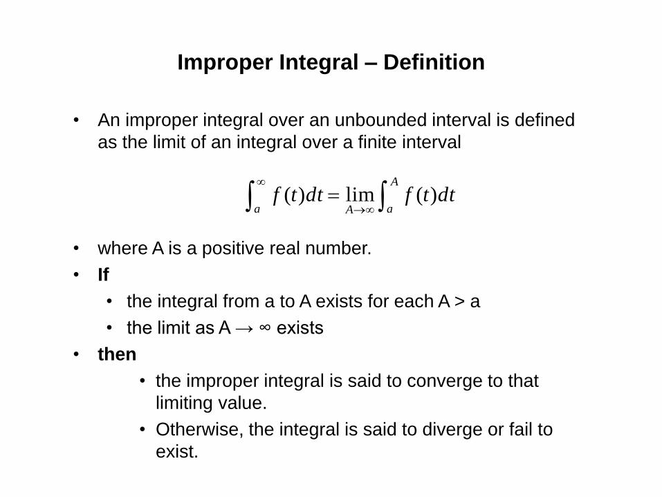
Improper Integral – Definition
• An improper integral over an unbounded interval is defined
as the limit of an integral over a finite interval
• where A is a positive real number.
• If
• the integral from a to A exists for each A > a
• the limit as A → ∞ exists
• then
• the improper integral is said to converge to that
limiting value.
• Otherwise, the integral is said to diverge or fail to
exist.
A
aAadttfdttf )(lim)(
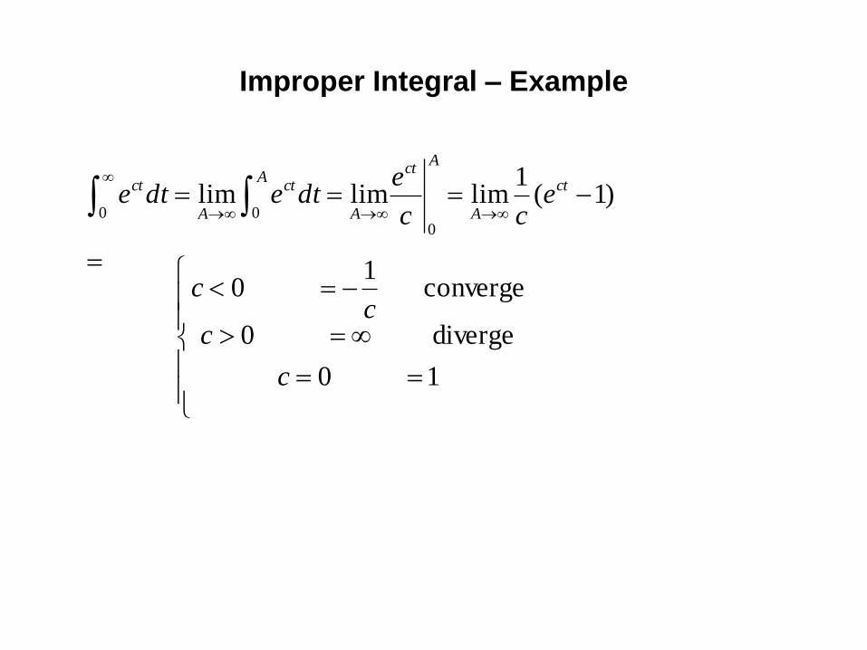
Improper Integral – Example
)1(1
limlimlim
000
ct
A
Act
A
Act
A
ct ecc
edtedte
10
diverge0
converge1
0
c
cc
c
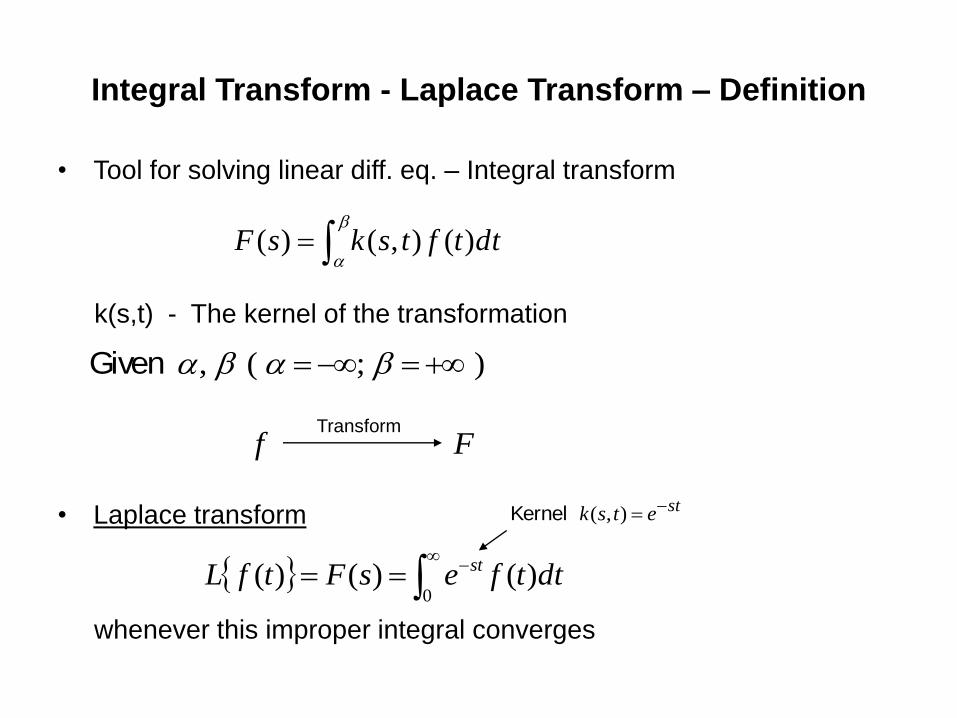
Integral Transform - Laplace Transform – Definition
dttftsksF )(),()(
• Tool for solving linear diff. eq. – Integral transform
k(s,t) - The kernel of the transformation
);(, Given
FfTransform
• Laplace transform
whenever this improper integral converges
0
)()()( dttfesFtfL st
stetsk ),(Kernel
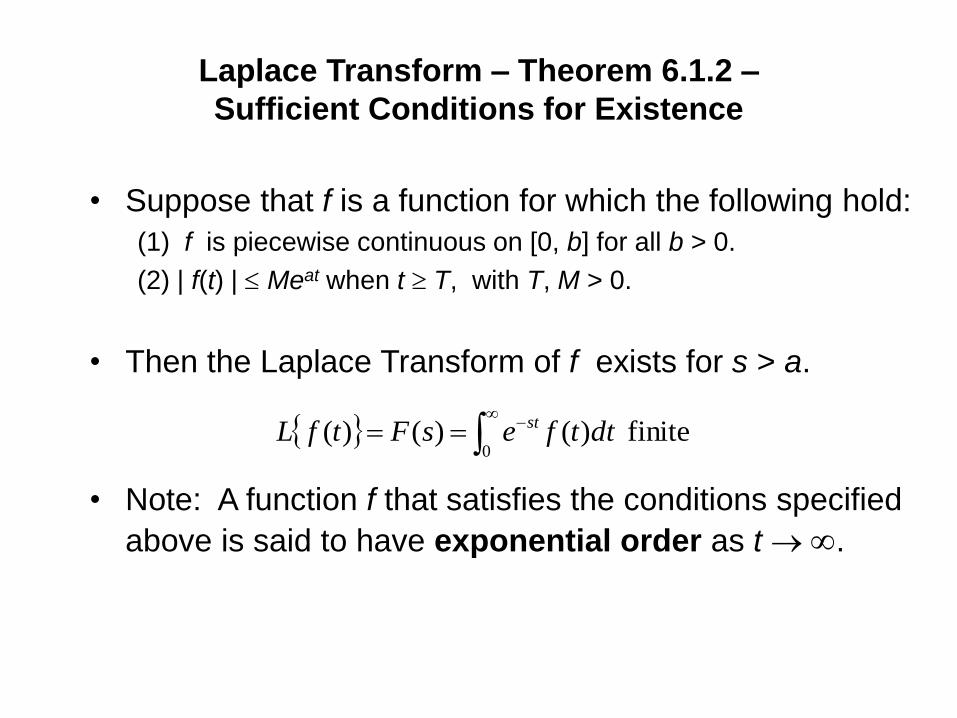
Laplace Transform – Theorem 6.1.2 –
Sufficient Conditions for Existence
• Suppose that f is a function for which the following hold:
(1) f is piecewise continuous on [0, b] for all b > 0.
(2) | f(t) | Meat when t T, with T, M > 0.
• Then the Laplace Transform of f exists for s > a.
• Note: A function f that satisfies the conditions specified
above is said to have exponential order as t .
finite )()()(0
dttfesFtfL st

Laplace Transform – Theorem 6.1.2 –
Condition No. 1 - Piecewise Continuous
• A function f is piecewise continuous on an interval [a,
b] if this interval can be partitioned by a finite number of
points
a = t0 < t1 < … < tn = b such that
(1) f is continuous on each (tk, tk+1)
• In other words, f is piecewise continuous on [a, b] if it is
continuous there except for a finite number of jump
discontinuities.
nktf
nktf
k
k
tt
tt
,,1,)(lim)3(
1,,0,)(lim)2(
1

Laplace Transform – Theorem 6.1.2 –
Condition No. 1 - Piecewise Continuous
2
2
1
1
)()()()(t
t
t
t
dttfdttfdttfdttf

Laplace Transform – Theorem 6.1.2 –
Condition No. 2 - Exponential Order
• If
– f is an increasing function
• Then
– | f(t) | Meat when t T, with T, M > 0.

Laplace Transform – Theorem 6.1.2 –
Condition No. 2 - Exponential Order
• A positive integral power of t is always of exponential order since
for c>0
tforMe
t
Met
ct
n
ctn
tet tt ee tet 2)cos(2

Laplace Transform (Function) – Example
1)(10
dtesFL st
ss
e
s
edteL
sA
A
Ast
A
st 11limlim11
00

Laplace Transform (Function) – Example
)(0
dteesFeL atstat
as
as
e
as
edtedteeeL
Aas
A
Atas
A
tasatstat
1
1limlim
)(
0
)(
0
)(
0

Laplace Transform (Function) – Example
)(0
dttesFtL st
2
000
0'
1111
1
11
0)1(
sssL
s
es
dts
e
s
tedttetL st
v
st
u
st
uv
st
dtuvuvdtvu
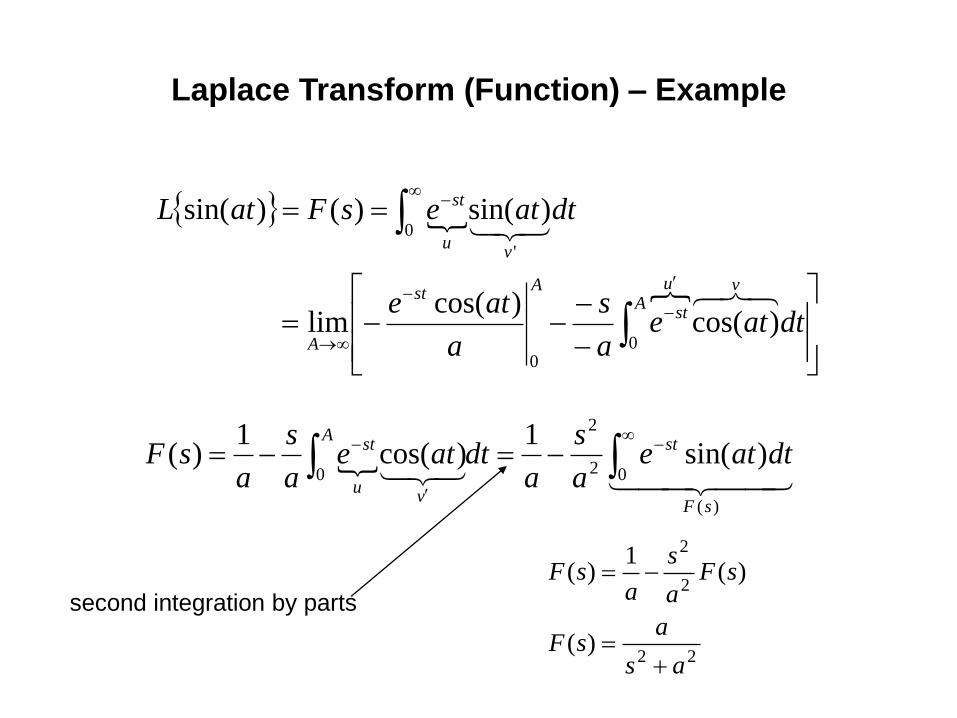
Laplace Transform (Function) – Example
Avu
st
Ast
A
vu
st
dtatea
s
a
ate
dtatesFatL
00
0
'
)cos()cos(
lim
)sin()()sin(
)(
02
2
0)sin(
1)cos(
1)(
sF
stA
vu
st dtatea
s
adtate
a
s
asF
second integration by parts
22
2
2
)(
)(1
)(
as
asF
sFa
s
asF

Laplace Transform – Discontinues Function - Example
• Transformation of piecewise continuous function
32
300)(
t
ttf
022
0
2)0()()(
3
0
0 3
3
0
ss
e
s
e
dtedtedttfetfL
sst
ststst

Operation Properties – Translation on the t-Axis (Time)
Second Translation Theorem
)()()( sFeatuatfL as
)()()()()( 11 atuatfatusFLsFeLatt
as

• Example:
Operation Properties – Translation on the S-Axis (Freq.)
First Translation Theorem
ass
at tfLasFtfeL
)()()(
)()()( 11 tfesFLasFL at
sas
4
55
335
)5(
6!3
ss
tLteLss
nss
t

Laplace Transform – Linearity
• Suppose f and g are functions whose Laplace
transforms exist for s > a1 and s > a2, respectively.
• Then, for s greater than the maximum of a1 and a2, the
Laplace transform of c1 f (t) + c2g(t) exists. That is,
with
finite is )()()()(0
2121
dttgctfcetgctfcL st
)( )(
)( )()()(
21
02
0121
tgLctfLc
dttgecdttfectgctfcL stst

Laplace Transform – Linearity – Example
)4sin(35 2 teL t
16
12
2
5
)4sin(35
2
2
ss
tLeL t


Inverse Laplace Transform – Example
4
5
1
5
1
24
1!4
!4
1
1t
SL
SL


Inverse Laplace Transform – Example
tS
LS
L 7sin7
1
7
7
7
1
7
12
1
2
1

Inverse Laplace Transform – Example
tt
SL
S
SL
SS
SL
S
SL
2sin32cos2
4
2
2
6
42
4
6
4
2
4
62
2
1
2
1
22
1
2
1
(linearity)
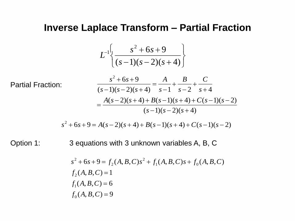
Inverse Laplace Transform – Partial Fraction
)4)(2)(1(
9621
sss
ssL
)4)(2)(1(
)2)(1()4)(1()4)(2(
421)4)(2)(1(
962
sss
ssCssBssA
s
C
s
B
s
A
sss
ss
)2)(1()4)(1()4)(2(962 ssCssBssAss
Partial Fraction:
Option 1: 3 equations with 3 unknown variables A, B, C
9),,(
6),,(
1),,(
),,(),,(),,(96
0
1
2
01
2
2
2
CBAf
CBAf
CBAf
CBAfsCBAfsCBAfss

Inverse Laplace Transform – Partial Fraction
)2)(1()4)(1()4)(2(962 ssCssBssAss
Option 2: Plug (s=1) 16=A(-1)(5) A=-16/5
Plug (s=2) 25=B(1)(6) B=25/6
Plug (s=-4) 1=C(-5)(-6) C=1/30
4
30/1
2
6/25
1
5/16
)4)(2)(1(
962
ssssss
ss
ttt eee
sL
sL
sL
sss
ssL
42
1112
1
30
1
6
25
5
16
4
1
30
1
2
1
6
25
1
1
5
16
)4)(2)(1(
96

Laplace Transform of a Derivative (First)
dttfestfe
dttfestfedttfetfL
stst
vu
st
vu
st
vu
st
)()()(
)()()()( )(
0
0
0
)0()()0()( )( fssFftfsLtfL
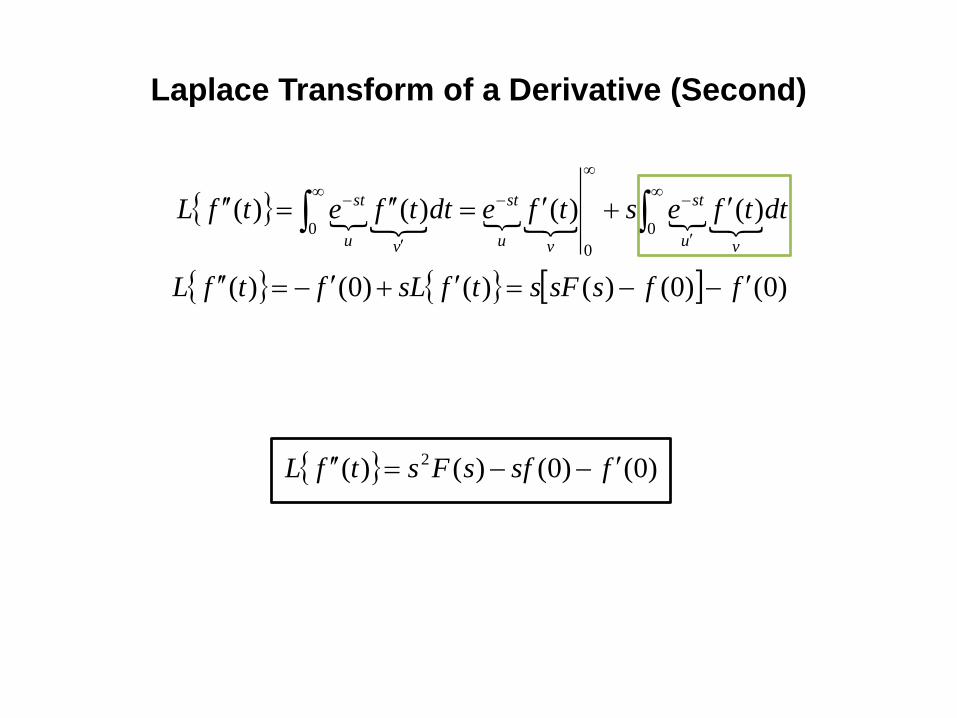
Laplace Transform of a Derivative (Second)
0
0
0)()()( )( dttfestfedttfetfL
vu
st
vu
st
vu
st
)0()0()()()0( )( ffssFstfsLftfL
)0()0()( )( 2 fsfsFstfL
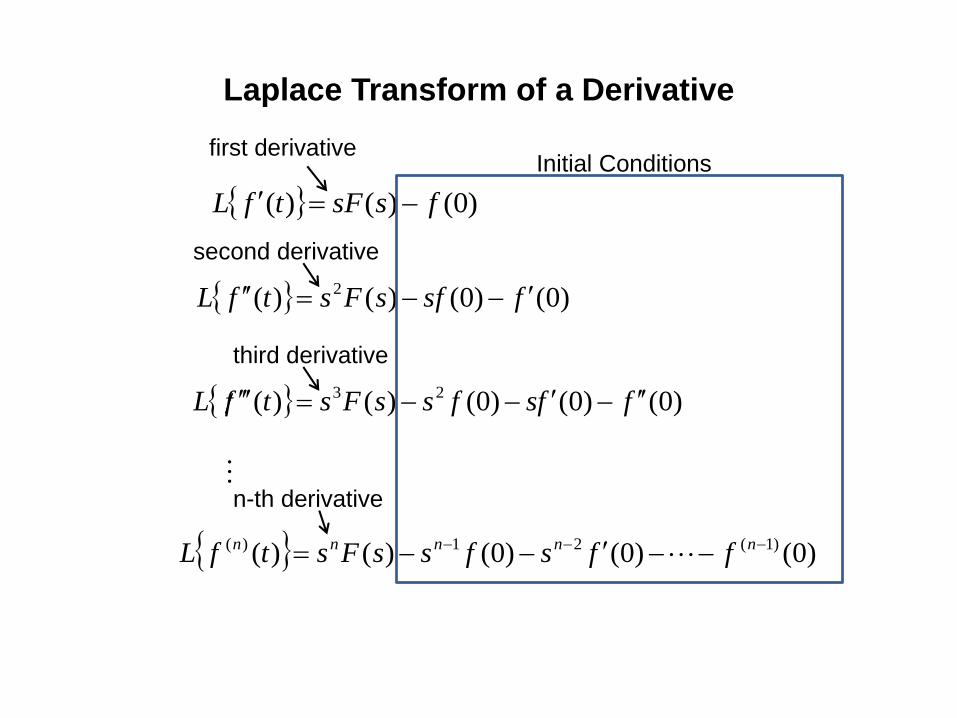
Laplace Transform of a Derivative
)0()( )( fssFtfL
)0()0()( )( 2 fsfsFstfL
)0()0()0()( )( 23 ffsfssFstfL
)0()0()0()( )( )1(21)( nnnnn ffsfssFstfL
first derivative
second derivative
third derivative
n-th derivative
Initial Conditions
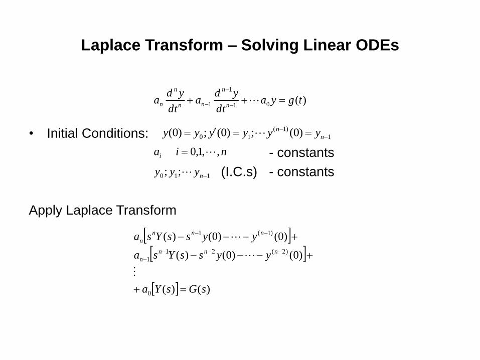
Laplace Transform – Solving Linear ODEs
• Initial Conditions:
- constants
(I.C.s) - constants
Apply Laplace Transform
)(01
1
1 tgyadt
yda
dt
yda
n
n
nn
n
n
1
)1(
10 )0(;)0(;)0(
n
n yyyyyy
110 ;; nyyy
niai ,,1,0
)()(
)0()0()(
)0()0()(
0
)2(21
1
)1(1
sGsYa
yyssYsa
yyssYsa
nnn
n
nnn
n

Laplace Transform – Solving Linear ODEs
• The Laplace Transform of a linear differential equation with constant
coefficients become an algebraic equation in Y(s)
Time Domain
Differential Equation
Frequency Domain
Algebraic Equation
Laplace Transform
I.C.
inputhomo-NonPolynimial
)()()()( sQsGsYsP
)(
)(
)(
)()(
sP
sQ
sP
sGsY
)(
)(
)(
)()()( 11
sP
sQ
sP
sGLsYLty
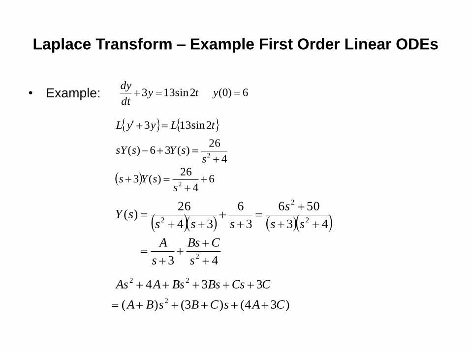
Laplace Transform – Example First Order Linear ODEs
6)0( 2sin133 ytydt
dy
tLyyL 2sin133
4
26)(36)(
2
ssYssY
64
26)(3
2
ssYs
43
43
506
3
6
34
26)(
2
2
2
2
s
CBs
s
A
ss
s
ssssY
)34()3()(
334
2
22
CAsCBsBA
CCsBsBsAAs
• Example:

Laplace Transform – Example First Order Linear ODEs
6
2
3
5034
03
6
C
B
A
CA
CB
BA
4
6
4
2
3
8
4
62
3
8)(
222
ss
s
ss
s
ssY
4
23
42
3
18)(
2
1
2
11
sL
s
sL
sLty
ttety t 2sin32cos28)( 3
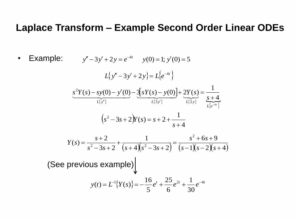
Laplace Transform – Example Second Order Linear ODEs
5)0( ;1)0( 23 4 yyeyyy t
teLyyyL 423
teLyLyLyL
ssYyssYysysYs
4
4
1)(2)0()(3)0()0()(
23
2
4
12)(232
sssYss
421
96
234
1
23
2)(
2
22
sss
ss
sssss
ssY
ttt eeesYLty 421
30
1
6
25
5
16)()(
• Example:
(See previous example)