landscape water budgeting manual (revised) of contents section 1. what is water budgeting? section...
TRANSCRIPT
Landscape Water Budgeting
(Class Manual for Online Training)
Currently Pending Approval for TCEQ Landscape Irrigation Credits
For Questions and Course Content: http://irrigation.tamu.edu
Online Access to Training: http://www.agrilifeirrigation.com

This page Intentionally Left Blank

This course and associated training materials were developed by the Texas A&M
School of Irrigation – Texas A&M AgriLife Extension Service under the direction of
Dr. Guy Fipps and Charles Swanson. All materials were developed for Educational
Purposes Only.
For Questions about course content, please contact:
Charles Swanson, Extension Program Specialist‐Landscape Irrigation
Dr. Guy Fipps, Professor & Extension Irrigation Engineer
For technical support and questions regarding registration & payment contact:
American Safety Council 1‐800‐732‐4135
Please note that students who complete this course as a requirement for TCEQ
Landscape Irrigation Licensing Programs Continued Education may only do so
once every licensing period. Students who repeat the training within the same
renewal period will not receive training credit.

This page Intentionally Left Blank

Table of Contents
Section 1. What is Water Budgeting?
Section 2. Determining the Water Requirements of Landscapes
Quiz 1
Section 3. Scheduling Concepts
Quiz 2
Section 4. Zoning Concepts
Quiz 3
Section 5. Precipitation Rate
Section 6. Landscape Water Budgeting
Section 7. GIS Based Tools for Water Balance
Section 8. Example of Water Budgeting on a Small Area City Use
Appendix A. Irrigation Water Management, Predicting Turf Water Requirements
Appendix B. ETo and rainfall data

Section 1 What is a Water Budget?


Section 2 Determining the Water
Requirements of Landscapes


Quiz 1:
1. KC may also be adjusted for such factors as:
A. Plant density
B. Desired plant quality
C. Level of stress
D. Site conditions
E. Micro‐climates
F. All of the above
2. Evapotranspiration, (ET) can’t be calculated using weather data.
o True
o False
3. Effective Rainfall includes the effects of slope, soil type, surface roughness
and other factors.
o True
o False
4. The methods that use solar radiation to calculate ET have proven to be the
most accurate.
o True
o False
5. Evapotranspiration, (ET) is very easy to measure directly.
o True
o False
6. The Adjustment Factor (Af): (Check all that apply)
o Is a modification to the crop coefficient
o Is used to balance or equations
o Is used to reduce water application for allowable stress

7. Water budgeting is usually an estimate of the amount of water to allocate to
landscape irrigation used for determination of: (Check all that apply)
o Estimated Applied Water Budgets
o Water wasted
o Water Use Tracking
o Maximum Applied Water Allowance
8. Irrigation scheduling calculations
A. Usually based on running a daily balance on ET, soil moisture levels and other factors
B. Usually based on a monthly or annual analysis
9. Water budgeting calculations
A. Usually based on running a daily balance on ET, soil moisture levels and other factors
B. Usually based on a monthly or annual analysis
10. Reference Evapotranspiration, ETo is also called the “Potential ET” (PET).
o True
o False
11. Crop coefficients (Kc) are used to relate ETo to the water requirements of
specific plants and crops.
o True
o False
12. The word evapotranspiration is a combination of the words “evaporation”
and “transpiration”.
o True
o False
13. If during the 1st week in Aug. 2007, Dallas received 0.04 inches of rainfall:
A. Since the total rainfall is equal to 0.04 inches, we assume no rainfall fell
B. Since the total rainfall is less than 0.1 inches, we assume no rainfall fell
C. Since the total rainfall is more than 0.01 inches, we assume no rainfall fell
D. Since the total rainfall is less than 0.3 inches, we assume no rainfall

14. Kc varies depending on the type of plant/crop and growth stage.
o True
o False
15. Water requirements (WR) can be adjusted for irrigation system efficiency
using Application efficiency (AE) and/or the Distribution.
o True
o False
16. The portion of rainfall that does not runoff, but becomes available for plant
water use is also known as _______.
A. Total Rainfall
B. Effective Rainfall
C. Rainfall Runoff
17. The Standardized Penman‐Monteith Equation is considered the less accurate
to calculate ETo.
o True
o False
18. Effective Rainfall considers how wet or dry the soil is.
o True
o False


Section 3 Scheduling Concepts


Irrigation Scheduling Worksheet USEFUL EQUATIONS
1. Water use = PET x Ax Kc 2. Available water = AWHC x Effective root zone depth
1. Refer to the ETo Table for 19 cities in Texas to answer the following questions.
a) What is the average monthly water requirement (in inches) in Dallas for a bermudagrass turf growing in July with a turf coefficient of 0.6 and an adjustment factor of 0.6?
b) What is the average daily water requirement (in inches)?
2. a) If a loam soil has an available water holding capacity of 1.8 in/ft, how much water
can be held within a 6‐inch root zone?
b) With an managed allowable depletion (MAD) of 50%, how much water can be depleted between irrigations?

c) With a average daily water use of 0.15 inches, how many days can you go between irrigations?
d) How much water (in inches) should be applied during each irrigation event?
3. a) Station 1 has a precipitation rate of 0.50 inches per hour. How long (in minutes)
must station 1 run for each irrigation in order to meet the turf water requirement 0.45 inches?
b) If station 2 has a precipitation rate of 0.75 inches per hour, how long must it be operate to apply 0.45 inches?
c) If station 3 has a precipitation rate of 0.50 inches per hour and has an application efficiency of 75%, how long must station 3 run to apply 1 inch of water over the entire area?

Quiz 2:
1. It determines the frequency of irrigation: (Check all that apply)
o Soil Type
o Weather
o Location
o Root zone depth
2. The concept of irrigation frequency is to: (Check all that apply)
o Wait to irrigate until the plants have depleted the water in the root zone
o Irrigate frequently to save water
o Irrigate as frequently as possible
o Run the irrigation system just long enough to fill back up the root zone
3. Irrigation frequency calculations are usually done on a monthly basis.
o True
o False
4. The process of irrigation frequency is:
A. First, calculate Irrigation Frequency (I), then, station runtime (RT) and the Plant Available
Water (PAW).
B. First, calculate Irrigation Frequency (IF), then, Running Time (RT) and the Plant Average
Water (PAW).
C. First, calculate the Plant Available Water (PAW), then calculate the irrigation Frequency
(I) and Station Runtime (RT).
5. On the equation for Plant Available Water PAW = D x SWHC x MAD:
PAW is used for_____ ____________________________________________________________
D is used for ___________________________________________________________________
SWHC is used for________________________________________________________________
MAD is used for_________________________________________________________________
A. The amount of water in the effective root zone available for plant uptake
B. The depth of the root zone that contains about 80% of the total root mass
C. The amount of water that can be held or stored in the soil
D. How dry the soil is allowed to become between irrigations (50% for most plants)
6. Effective Root Zone:
A. The depth containing about 80% of the total root mass
B. Excludes “tap” and “feeder” roots
C. Easily measured with a soil probe
D. All of the above
7. The amount of water that can be held or stored per yard of soil depth is the
soil water holding capacity.
o True
o False
8. Station Runtime definitions:
Precipitation Rate
A. How long a station is operated during an irrigation event
B. Sprinkler group on a common valve that may be part of an automated irrigation system
that operates at the same time
C. Measurement in inches per hour of how fast an irrigation system applies water to a
landscape

Station
A. How long a station is operated during an irrigation event
B. Sprinkler group on a common valve that may be part of an automated irrigation system
that operates at the same time
C. Measurement in inches per hour of how fast an irrigation system applies water to a
landscape
Runtime
A. How long a station is operated during an irrigation event
B. Sprinkler group on a common valve that may be part of an automated irrigation system
that operates at the same time
C. Measurement in inches per hour of how fast an irrigation system applies water to a
landscape
9. The following equation I = WR / PAW is:
o True
o False
10. The amount of water in the effective root zone “available” for plant uptake
is the plant available water.
o True
o False


Section 4 Zoning Concepts


Quiz 3:
1. Inadequate flow rate for the number of sprinkler heads is a:
A. Characteristic of a poorly zoned landscape
B. Characteristic of a poorly designed station
2. Mixed sprinkler heads (types) is a:
A. Characteristic of a poorly zoned landscape
B. Characteristic of a poorly designed station
3. The zoning is defined by the Annual Growth Response.
o True
o False
4. The zoning is defined by the characteristics of the soil.
o True
o False
5. Impractical turf areas are a:
A. Characteristic of a poorly designed station
B. Characteristic of a poorly zoned landscape
6. A station is determined by: (Check all that apply)
o Soil characteristics
o Available flow and pressures
o Plant water needs
o Application device (sprinkler type)
o Sun exposure / micro‐climates

7. Precipitation rate inappropriate for the soil type is a:
A. Characteristic of a poorly zoned landscape
B. Characteristic of a poorly designed station
8. Impractical shrub and tree plantings are a:
A. Characteristic of a poorly designed station
B. Characteristic of a poorly zoned landscape
9. Grouping plants by water use:
Regular Watering Zone___________________________________________________________
Occasional Watering Zone________________________________________________________
Natural Watering Zone___________________________________________________________
A. Requires watering once every week or more ONCE ESTABLISHED, in the absence of rain
B. Requires watering once every two or three weeks ONCE ESTABLISHED, in the absence of
rain
C. Requires only natural rainfall ONCE ESTABLISHED except for periods of drought
10. For Regular Watering Zone, the plants included are turfgrasses and flowers.
o True
o False
11. The zoning is defined by:
A. Maintenance requirements
B. Exposure to sun
C. Size/shape of the landscape
D. All of the above
12. Excessive pressure loss in the pipe system is a:
A. Characteristic of a poorly designed station
B. Characteristic of a poorly zoned landscape

13. A zone in an irrigation system is defined by such factors as: (Check all that
apply)
o Application device (sprinkler type)
o Sun exposure/micro climates
o Soil characteristics
o Plant water needs
o Available flow and pressures
14. Plant types of mixed water requirements and growth characteristics are:
A. Characteristics of a poorly designed station
B. Characteristics of a poorly designed landscape
15. The zoning is defined by the Plant Water Needs.
o True
o False
16. For Natural Watering Zones the plants included are: vines, tough woody
shrubs and established shade trees.
o True
o False
17. Poor DU is a:
A. Characteristic of a poorly designed station
B. Characteristic of a poorly zoned landscape

Section 5 Precipitation Rate


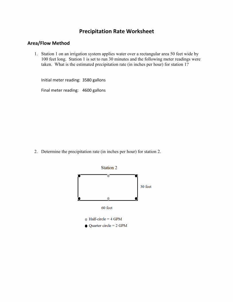
Precipitation Rate Worksheet
Area/Flow Method
1. Station 1 on an irrigation system applies water over a rectangular area 50 feet wide by 100 feet long. Station 1 is set to run 30 minutes and the following meter readings were taken. What is the estimated precipitation rate (in inches per hour) for station 1?
Initial meter reading: 3580 gallons
Final meter reading: 4600 gallons
2. Determine the precipitation rate (in inches per hour) for station 2.

Catch Can Method
1. A catch can test was conducted for station 4 using a conical shaped catch device with a “throat” opening area of 15 square inches. The following catch can volumes were recorded (in milliliters) over a 10 minute period:
Catch Can Volumes (milliliters)
45 32 43 33 39 54 23 51 28 22 43 22
What is the precipitation rate (in inches per hour) for station 3?
2. A catch can test was conducted for station 4. The following 12 can depths were recorded over a 30 minute period:
Catch Can Depth ‐ Inches
0.7 0.8 0.5 0.6 0.5 0.9 0.4 0.5 0.6 0.6 0.7 0.7
What is the precipitation rate (in inches per hour) for station 4?
Section 6 Landscape Water Budgeting


3

Water Budgeting Worksheet
1. What is the total landscape area for my residence located in Bryan, Texas (in ft2)?
Lot size ‐ 1/3 acre
residence ‐ 2200 ft2
detached garage ‐ 1520 ft2
hard space (driveway, patio, walkways) ‐ 30% of yard area
2. The landscape area of my residence is primarily turf (St. Augustine):
Produce an Estimate Applied Water Budget for the month of July for the
following three cases:
A. Worst Case
B. Expected Use
C. Maximum Conservation

3. Considering indoor water use, what is my total expected water use in July
considering expected in‐door use?


Section 7 GIS‐ Based Tools for Water Budgeting


Section 8 Example of Water Budgeting on a
Small Area for City Use


1. This im
age shows an
aerial photography of the sm
all city and surrounding
area. In the left m
enu is the ID number of the aerial photograph. Also, as shown
in the left m
enu, w
e are view
ing the im
age in all three colors
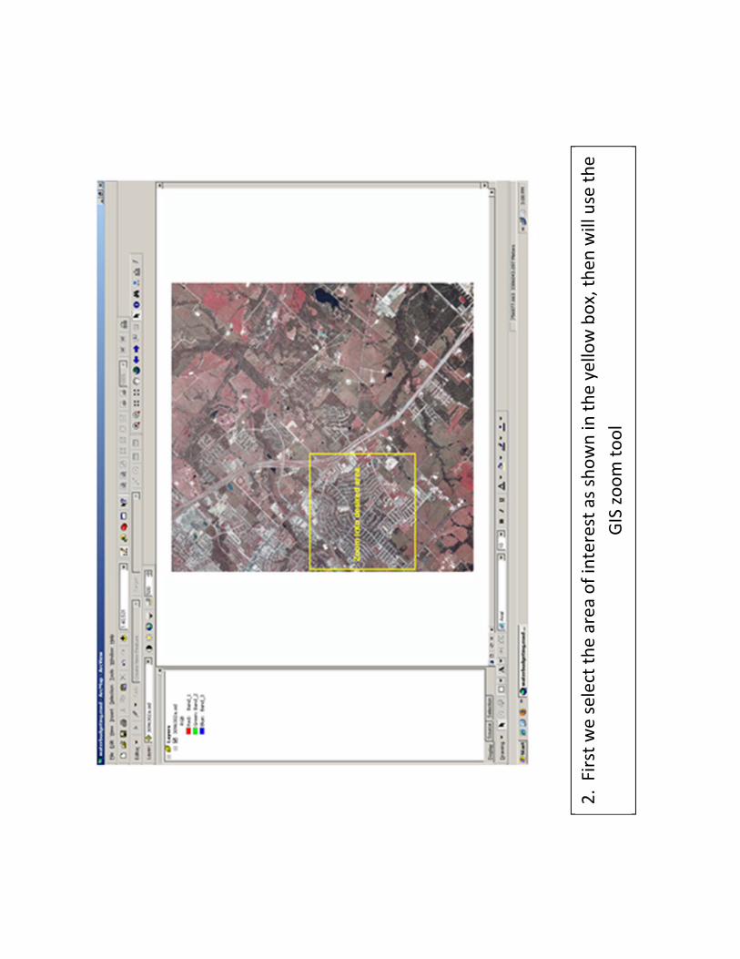
2. First we select the area
of interest as shown in
the yellow box, then
will use the
GIS zoom tool

3. Now we can m
ake out the streets and individual houses and yards. W
e will
select a smaller area
to work with

4. The area
highlighted in
yellow is where we will conduct our analysis. We again
use the GIS zoom tool to display this area.

5. In this area, all the streets, houses and yards are laid out in the same pattern.

6. The area
highlighted in
yellow is the first of three areas (or blocks) of houses
and yards that we will use. Using the GIS drawing tool, we map
this area and add
the block layer to the GIS as seen
in the left m
enu.

7. We map
the next area

8. We map
the final area.
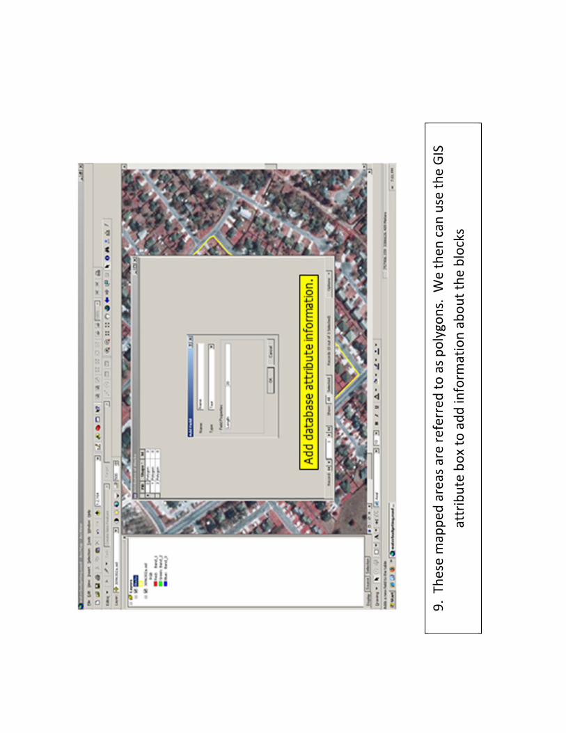
9. These mapped
areas are referred to as polygons. W
e then
can
use the GIS
attribute box to add inform
ation about the blocks

10. The nam
e or location of the block is usually entered. Here we will label these
as blocks 64, 65 and 66.

11. For water budgeting, w
e need to determine the landscape area. First we will
determine the total area of each block. There are several different ways to do this
in GIS. Here, we are using the calculate area tool.

12. As area
is calculated, a status box is displayed.

13. W
e now have a new
map
(or shapefile) which is added
to our GIS containing
the boundaries and area of each block.

14. Right clicking on the shapefile brings up a m
enu with several options. H
ere
we select the Open
Attribute Table option
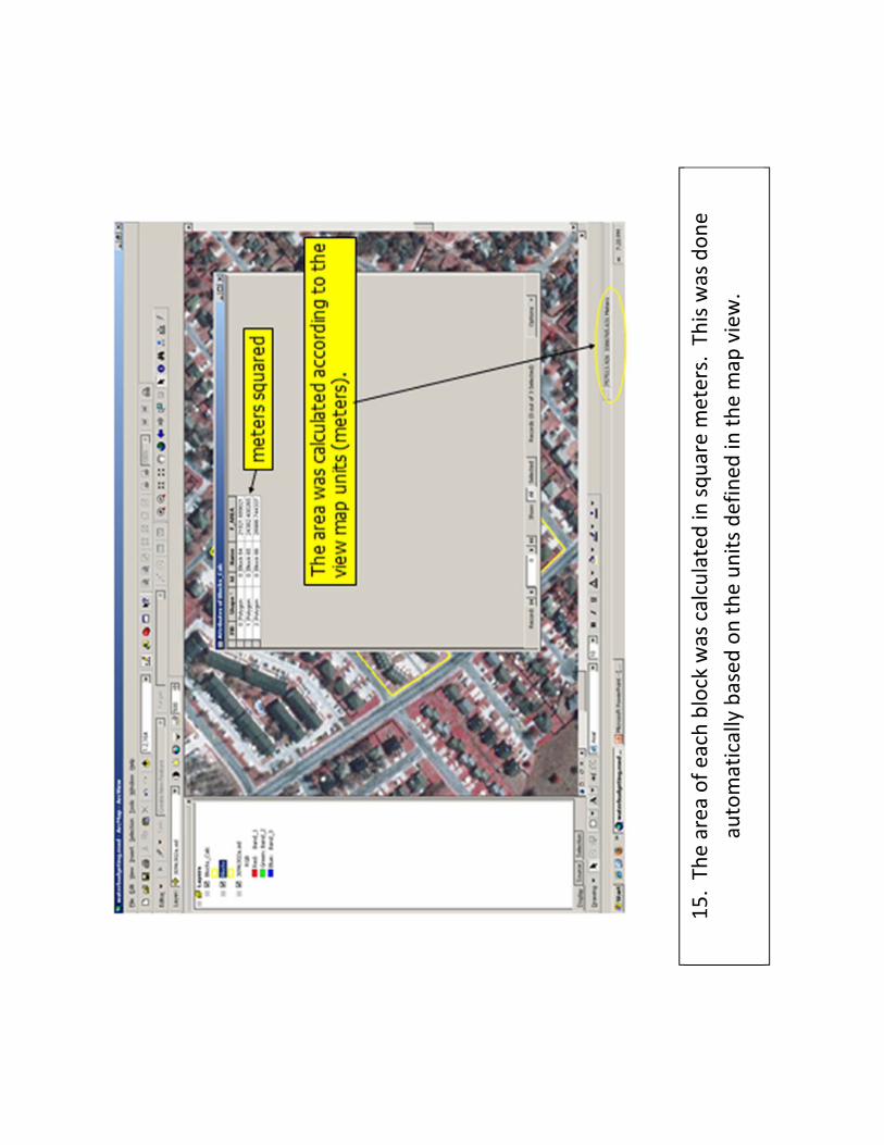
15. The area
of each block was calculated in
square meters. This was done
automatically based
on the units defined
in the map
view.
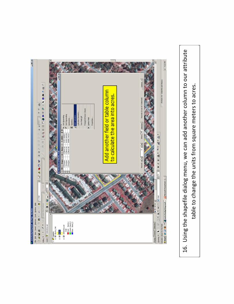
16. Using the shapefile dialog men
u, w
e can add another column to our attribute
table to change the units from square meters to acres.

17. In the field calculation dialog men
u, w
e can add equations to do any
calculation we wish. Here we use the conversion factor for square meters to
acres.

18. The area
of each block in
acres has been added
to our attribute table.

Determ
ining the Irrigation Acreage vs. Total A
creage
•Method 1: U
sing the tool to cut the polygon into pieces is one way to
separate out lawn vs. hard surface areas

For water budgeting, we need to know the total landscape area. So, w
e need to
remove the areas covered by houses, driveways, sidew
alks and other hard spaces.
We will use the Cut Polygon Features tool to do this.

Using the cut tool, we draw out the upper boundary of the alley.
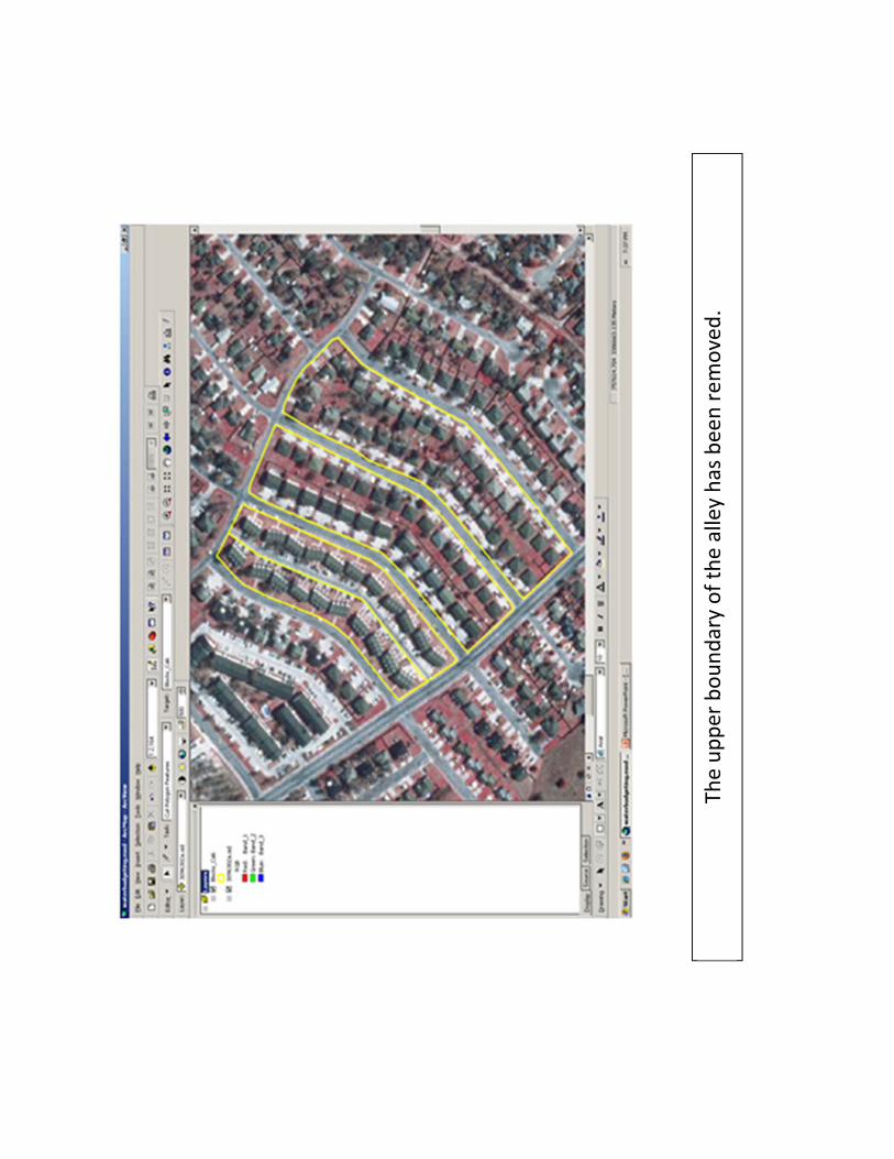
The upper boundary of the alley has been rem
oved.

We repeat the process for the lower boundary of the alley.

Now that the alley has been cut out of the area, the attribute table is updated
with the new
area.

Usually, just the general boundaries of the alley are good enough
for city‐w
ide
calculations. H
owever, w
e can im
prove the accuracy by excluding the driveways
and parking areas for each house.

For this example, w
e will use a different procedure, m
apping of the alley and
driveways. First, w
e will draw the boundaries of the driveways along one side of
the alley.

and we complete the map
of the alley and driveways by drawing the boundaries
along the lower side.

This m
ap or outline of the alley and driveways is referred to as a polygon in
GIS.
Using the measure tool, we can determine the areas.
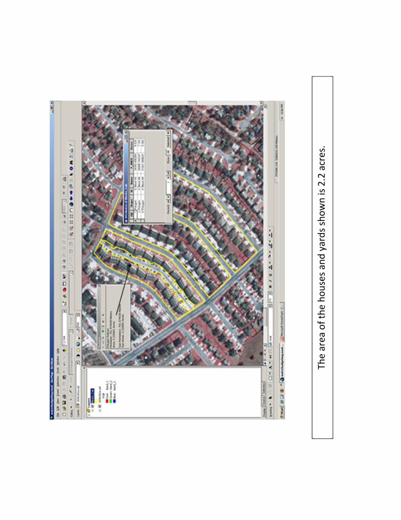
The area
of the houses and yards shown is 2.2 acres.

The area
of the alley and driveway is 1.15 acres.

The area
of the bottom row of houses and yards is 2.02 acres.

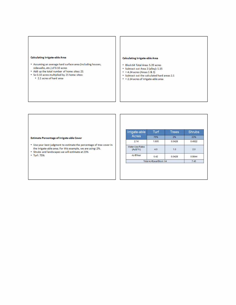
Block 64 Area
•Area 1 (top): 2.22
•Area 2 (alley): 1.15
•Area 3 (bottom): 2.02
•Total A
rea: 5.39 acres

The next step
is to exclude the areas covered by the houses, walkw
ays and other
hard spaces. To
do this, w
e select four properties and m
ap them
out with the
measuremen
t tool.

The measuremen
t tool gives us the areas of the houses and walkw
ays.

This im
age shows the four properties we mapped
and their corresponding areas.

Other areas do not require cutting out large
non‐irrigate‐able areas such as the next block.


Appendix A Irrigation Water Management
Predicting Turf Water Requirements


IRRIGATION WATER MANAGEMENT
PREDICTING TURF WATER REQUIREMENTS
Step 1: Determine Local ETo Step 2: Select Crop Coefficient (Kc)
Step 3: Determine Adjustment Factor (Af) Step 4: Calculate Water Requirement
Definitions Adjustment Factor (Af) - a modification of the crop coefficient (in percent). An adjustment factor is used to reduce water application for allowable stress, for microclimates such as excessive shade or sun, and personal preference of the landscape manager. Allowable stress - a factor which reflects an “acceptable” turf quality under reduced water supply. Allowable stress varies by individual preference and the requirements of the location. Research has shown that turf water supply can be reduced by 40% or more and still maintain acceptable appearance for most sites. Cool season turfgrasses - turfgrasses adapted to cooler climates such as tall fescue and ryegrass. Evapotranspiration (ET) - a measurement of the total water needs of plants including the water lost to the atmosphere through evaporation of water from the soil surface and transpiration through the plant. Potential evapotranspiration (ETo) - the potential water use of a cool season grass, growing four inches tall under well-watered conditions. It is used as a reference to which the water requirements of other plants can be related. ETo varies with climate as a function of temperature, relative humidity, wind speed and solar radiation. Different locations have different ETo rates due to changes in climate. (ETo is sometimes written as “PET”.) Crop coefficient (Kc) - a factor used to relate ETo to the actual water use for a specific plant or turf type. The crop coefficient, Kc, reflects the percentage of ETo that a specific plant or turf type requires for maximum growth (such as for growing Bermuda grass hay). Warm season turfgrasses - turfgrasses adapted to warmer climates such as Bermuda grass, St. Augustine grass and Zoysia grass.
1

QUICK-TABLE A. Turf Water Requirement # Variable Value Units Source 1 Potential Evapotranspiration
(ETo) 7.96 inches per
month Appendix A - ETo Table
2 Crop Coefficient (Kc) 0.6 decimal Appendix A - Kc Table 3 Adjustment Factor (Af) 1 decimal Site specific, professional
judgment (shade, slope, etc.)
4 Water Requirement (WR)1 4.78 inches per month
#1 x #2 x # 3
1Water requirement for a warm season turfgrass grown in San Antonio in the month of July (assuming no rainfall).
Detailed Instructions for Predicting Turf Water Requirements Step 1: Determine Local ETo - Appendix A gives average monthly ETo for 19 major cities in Texas. The Agricultural Program of Texas A&M University System has ETo networks that report current daily ETo throughout Texas on the Internet, web address: http://texaset.tamu.edu. Step 2: Select Crop Coefficient (Kc) - Warm season turfgrasses use up to 60% of ETo, while cool season grasses can use up to 80% of ETo. Appendix A gives monthly Kc values for the 19 major cities in Texas for warm season, cool season, and warm season turfgrasses overseeded with ryegrass. Step 3: Determine Adjustment Factor (Af) - The Kc represents the maximum amount of ETo that turfgrasses will use. However, many plants, especially turfgrass, exhibit the ability to survive on much less water without showing signs of stress or a reduction in quality. For this reason the crop coefficient is adjusted to represent “allowable stress”. For example, buffalo grass has shown to survive on much less water than St. Augustine grass, though they are both warm season grasses. Thus, Af for buffalo grass may be as low as 0.4, while Af for St. Augustine grass may only reach 0.6. Microclimates will also influence water use, especially in small landscapes. Certain areas around buildings or under trees may receive more shade, and therefore require less water than areas under full sun. Wind speed also influences water use. For example, areas between buildings may experience a “venturi effect” resulting in high winds that increase plant transpiration. To make up for such losses, more water must be applied.
2

Step 4: Calculate Water Requirement - Water use in turfgrasses is calculated using the following relationship:
WR= ET K Ao c f (Equation 1) where: WR - Water requirement (inches)
ETo - Potential evapotranspirationinches
day
inches
week
inches
month
, , or
Kc - Crop coefficient (decimal) Af - Adjustment factor (decimal)
Example 1: ETo = 7.96 inches per month
Kc = 0.6 Af = 1
WR = 4.78 inches per month
DETERMINING IRRIGATION FREQUENCY
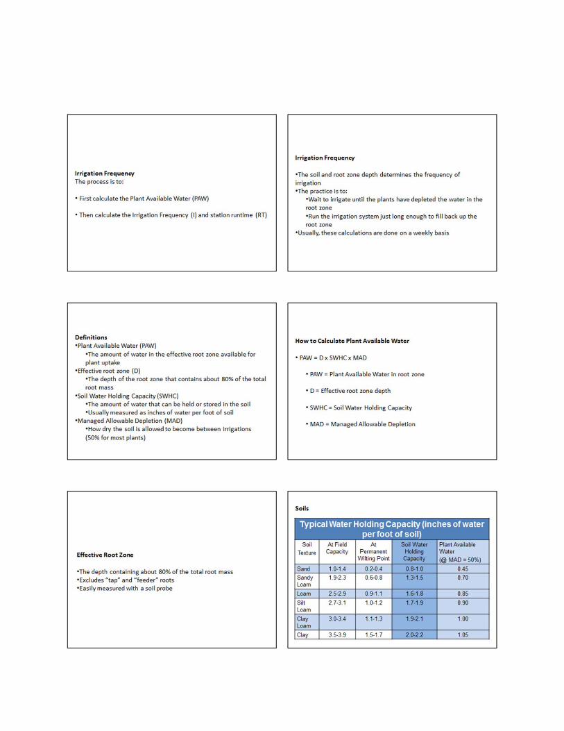
Step 1: Measure Effective Root Zone Step 2: Determine Soil Type and Soil Water Holding Capacity Step 3: Calculate Plant Available Water (PAW) Step 4: Calculate Irrigation Frequency Definitions Plant available water - the amount of water in the soil (in inches) that is “available” for plant uptake. (Determined by the difference in moisture content at field capacity and the permanent wilting point times managed allowable depletion or MAD). Effective root zone - the depth of root zone (in inches) containing approximately 80% of the total root mass. Irrigation frequency - the number of irrigation events per week. Managed allowable depletion (MAD) - the process of letting the soil dry out to a prescribed soil moisture level between irrigations (50% for most turfgrasses). Soil type (texture) - classification of soils into categories such as sand, clay, loam, etc. Soil water holding capacity - the amount of water (in inches) that can be “held” or stored per foot of soil depth.
3

QUICK TABLE B. Irrigation Frequency # Variable Value Units Source1 Effective Root Zone Depth (D) 5 inches soil Soil probe
measurements 2 Soil Water Holding Capacity
(SWHC) 1.8 inches per foot Table 1, loam soil
3 Managed Allowable Depletion (MAD)
0.5 decimal MAD for turf (50%)
4 Plant Available Water (PAW) 0.38 inches of water (#1 ÷ 12 inches/foot) x #2 x #3
5 Monthly Water Requirement (WR)
4.78 inches per month QUICK TABLE A
6 Weekly Water Requirement (WR)
1.2 inches per week #5 ÷ 4 weeks
7 Irrigation Frequency (I) 4 number of irrigations per week
#6 ÷ #4, rounded to next whole number
Detailed Instructions for Determining Irrigation Frequency Step 1: Measure Effective Root Zone - Many factors restrict root development. Depths may vary because of physiological differences of plants. Other factors that influence root zone depth include high water tables, shallow soils, changes in soil type, compaction, irrigation, fertilization and cultural practices. For irrigation scheduling, we use the effective root zone depth. This is the depth that contains about 80% of the total root mass and excludes the deeper “tap” or “feeder” roots. In order to obtain an accurate determination of root zone depth, samples should be taken in several locations since the soil type and composition can vary significantly within a landscape. Step 2: Determine Soil Type and Soil Water Holding Capacity - Soil types vary in the amount of water that can be "stored" or "held" in the root zone. Fine textured soils, such as clays have high soil water holding capacities, while coarse textured soils, such as sands, exhibit low soil water holding capacities. Table 1 gives typical water holding capacities by soil type in inches of water per foot of soil.
4
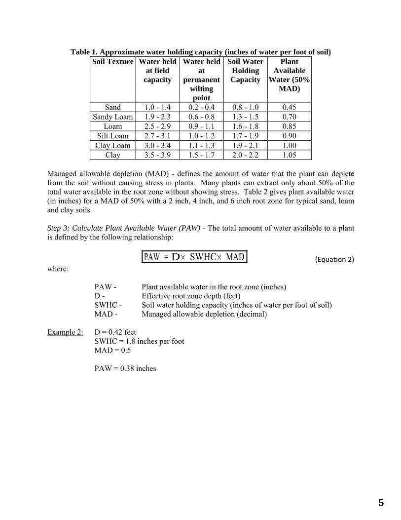
Table 1. Approximate water holding capacity (inches of water per foot of soil) Soil Texture Water held
at field capacity
Water held at
permanent wilting point
Soil Water Holding Capacity
Plant Available
Water (50% MAD)
Sand 1.0 - 1.4 0.2 - 0.4 0.8 - 1.0 0.45 Sandy Loam 1.9 - 2.3 0.6 - 0.8 1.3 - 1.5 0.70
Loam 2.5 - 2.9 0.9 - 1.1 1.6 - 1.8 0.85 Silt Loam 2.7 - 3.1 1.0 - 1.2 1.7 - 1.9 0.90 Clay Loam 3.0 - 3.4 1.1 - 1.3 1.9 - 2.1 1.00
Clay 3.5 - 3.9 1.5 - 1.7 2.0 - 2.2 1.05 Managed allowable depletion (MAD) - defines the amount of water that the plant can deplete from the soil without causing stress in plants. Many plants can extract only about 50% of the total water available in the root zone without showing stress. Table 2 gives plant available water (in inches) for a MAD of 50% with a 2 inch, 4 inch, and 6 inch root zone for typical sand, loam and clay soils. Step 3: Calculate Plant Available Water (PAW) - The total amount of water available to a plant is defined by the following relationship:
PAW = D SWHC MAD (Equation 2) where:
PAW - Plant available water in the root zone (inches) D - Effective root zone depth (feet) SWHC - Soil water holding capacity (inches of water per foot of soil) MAD - Managed allowable depletion (decimal)
Example 2: D = 0.42 feet
SWHC = 1.8 inches per foot MAD = 0.5
PAW = 0.38 inches
5

Table 2. Plant available water for 3 root zone depths at 50% MAD.
Soil Texture
Soil Water Holding Capacity
(inches water per foot of
soil)
Available Water @
50% MAD (inches water
per foot of soil)
Available Water @
50% MAD (inches water
per inch of soil)
Total Plant Available Water
(inches water) 2" Root
Zone 4" Root
Zone 6" Root
Zone
Sand 0.90 0.45 0.038 0.076 0.15 0.23 Loam 1.70 0.85 0.071 0.14 0.28 0.43 Clay 2.10 1.05 0.088 0.18 0.35 0.53
Step 4: Calculate Irrigation Frequency - Irrigation frequency is determined on a weekly basis. The number of irrigations per week is calculated from the total weekly water requirement and the amount of plant available water as follows:
I =
WR
PAW ( Equation 3) where:
I - Number of irrigations per week (rounded to next whole number) WR - Water requirement (inches per week) PAW - Plant available water in root zone (inches)
Example 3: WR = 1.2 inches per week
PAW = 0.38 inches I = 4 irrigations per week
6

DETERMINING STATION RUN TIMES
Step 1: Calculate Turf Water Requirement Step 2: Calculate Plant Available Water (PAW)
Step 3: Calculate Irrigation Frequency Step 4: Determine Precipitation Rate (PR)
Step 5: Calculate Station Run Time
Definitions Precipitation rate - measurement of how fast an irrigation system applies water to a landscape in inches per hour. Stations - group of sprinklers on an automated irrigation system that operate at the same time. Run time - how long a station is operated during an irrigation event.
QUICK-TABLE C. Station Run Times # Variable Value Unit Source
1 Turf Water Requirement (WR) 1.2 inches per week
QUICK-TABLE B: #6
2 Irrigation Frequency (I) 3 number of irrigations per week
QUICK-TABLE B: #7
3 Precipitation Rate (PR) 1.0 inches per hour Measured with catch devices, or other method
4 Station Run Time (RT) 24 minutes (#1 x 60) ÷ ( #2 x #3) Detailed Instructions for Determining Station Run Time Step 1: Calculate Turf Water Requirement - (see page 3) Step 2: Calculate Plant Available Water (PAW) - (see page 5) Step 3: Calculate Irrigation Frequency - (see page 6)
7

Step 4: Determine Precipitation Rate (PR) - Precipitation rate is a measurement of how fast an irrigation system applies water to a landscape. There are three primary methods for determining precipitation rates: manufacturers specifications, catch can tests, and meter readings. Details are provided in the next section. Station precipitation rates often vary within an irrigation system due to such factors as poor sprinkler alignment, spray trajectory and pressure fluctuations. Different types of irrigation equipment have different precipitation rates, it is necessary to determine the precipitation rate of each station on an irrigation system. Step 5: Calculate Station Run Time - Station run times can be calculated from water requirement, irrigation frequency and precipitation rate using the following equation:
RT =
WR
I PR 60
(Equation 4) where:
RT - Station run time (minutes) WR - Water requirement (inches per week) I - Number of irrigations per week PR - Precipitation rate (inches per hour)
Example 4: WR = 1.2 inches per week
I = 3 irrigation per week PR = 0.5 inches per hour
RT = 48 minutes
DETERMINING PRECIPITATION RATE Definitions Catch device - a container used to measure the amount of water an irrigation system applies, commonly referred to as a “catch can”. Coverage area - the landscape area covered by a single sprinkler head or contained within a station, in square feet (ft2). GPM - flow rate of water through an irrigation system expressed in gallons per minute (gpm).
8

Heads - sprinkler application devices used to apply water to a landscape; the most common are sprays, rotors and impacts. Station - individual or multiple sprinkler heads on an irrigation system usually activated by a single solenoid valve connected to a central controller. Testing run time - the total time that each station is operated during catch can tests. Throat area - the surface area of the top of a catch device through which the water falls, in square inches (in2). Water meters - devices used to meter the volume of water that flows through a piping system, commonly in units of gallons or cubic feet (ft3, cf). A. Catch Can Method
Step 1: Select Catch Device Step 2: Determine Throat Area
Step 3: Identify Stations and Locations of Heads Step 4: Lay Out Catch Devices
Step 5: Run Each Station Step 6: Record Catch Volumes
Step 7: Calculate Precipitation Rate Step 1: Select Catch Device - A catch device "catches" the irrigation water during a test and holds it for measurement. Catch devices range from special graduated conical cylinders to tuna fish cans. Some devices have raised graduation marks which allow the volume to be read directly. With other devices, the water that is caught is poured into a graduated cylinder, and the volume is then measured. Irrigation depth in straight-sided devices, such as a tuna can, may be estimated directly using a ruler; however, this method is not always practical since it requires long testing run times in order to collect a sufficient depth of water necessary for accurate measurements. Step 2: Determine Throat Area: The "throat area" is the size of the top of the catch device in square inches. For round catch devices, the throat area is calculated as follows:
Ad
4
2
where A = throat area (square inches, in2) and d = diameter (inches, in), and � = 3.14 (constant). Step 3: Identify Stations and Locations of Heads - Identify the location of each sprinkler head in a station by briefly running each station on the controller. Place colored flags to mark all heads. It is helpful to use a different color for each station (e.g., red flags for station 1, green flags for station 2).
9
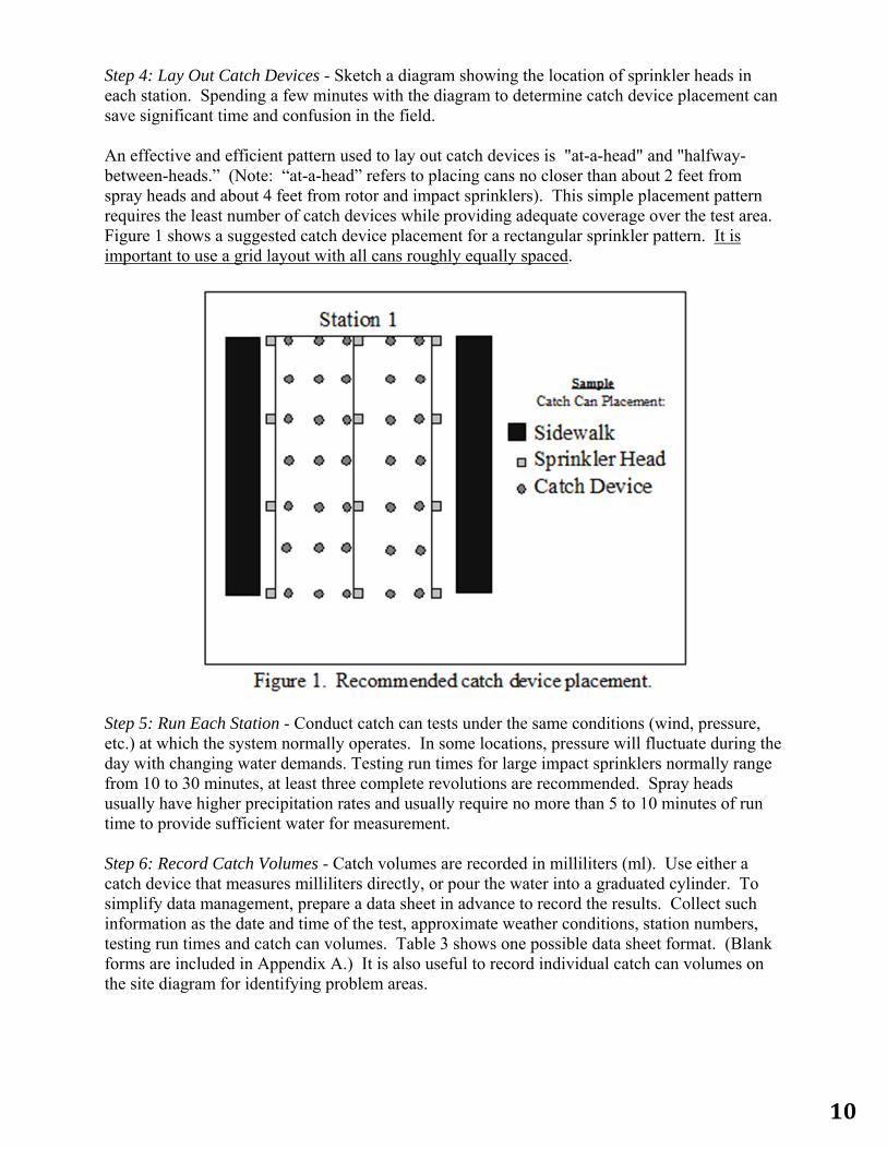
Step 4: Lay Out Catch Devices - Sketch a diagram showing the location of sprinkler heads in each station. Spending a few minutes with the diagram to determine catch device placement can save significant time and confusion in the field. An effective and efficient pattern used to lay out catch devices is "at-a-head" and "halfway- between-heads.” (Note: “at-a-head” refers to placing cans no closer than about 2 feet from spray heads and about 4 feet from rotor and impact sprinklers). This simple placement pattern requires the least number of catch devices while providing adequate coverage over the test area. Figure 1 shows a suggested catch device placement for a rectangular sprinkler pattern. It is important to use a grid layout with all cans roughly equally spaced.
Step 5: Run Each Station - Conduct catch can tests under the same conditions (wind, pressure, etc.) at which the system normally operates. In some locations, pressure will fluctuate during the day with changing water demands. Testing run times for large impact sprinklers normally range from 10 to 30 minutes, at least three complete revolutions are recommended. Spray heads usually have higher precipitation rates and usually require no more than 5 to 10 minutes of run time to provide sufficient water for measurement. Step 6: Record Catch Volumes - Catch volumes are recorded in milliliters (ml). Use either a catch device that measures milliliters directly, or pour the water into a graduated cylinder. To simplify data management, prepare a data sheet in advance to record the results. Collect such information as the date and time of the test, approximate weather conditions, station numbers, testing run times and catch can volumes. Table 3 shows one possible data sheet format. (Blank forms are included in Appendix A.) It is also useful to record individual catch can volumes on the site diagram for identifying problem areas.
10

Table 3. Sample Data Collection SheetSite Name: Beaver Park Start Time: 8:30 a.m. Date: 8/8/97 End Time: 10:30 a.m. Station number 1 2 3 Testing run time (minutes) 10 15 5 Catch volume (milliliters) 24, 22 35, 42 10, 14 20, 32 54, 43 11, 15 21, 25 55, 38 16, 8 30, 28 44, 48 10, 15 22, 20 40, 42 12, 15 Temperature: 80 F Wind speed/direction: 0 RH: 60%
Step 7: Calculate Precipitation Rate - Calculate the precipitation rate of each station using the following equation:
PR =
V 3.6612
n a tt R
(Equation 5)
where: PR - Precipitation rate (inches per hour)
�V - Summation of all catch can volumes (milliliters) 3.6612 - Constant, converts milliliters to cubic inches and minutes to hours n - Number of catch devices at - Throat area of catch device (square inches) tR - Testing run time (minutes)
Example 5: For Station 1 above.
�V = 244 milliliters n = 10 at = 16.61 square inches tR = 10 minutes
PR = 0.54 inches per hour
11

B. Area/Flow Method
Step 1: Determine the Flow Rate of Each Station Step 2: Determine Coverage Area
Step 3: Calculate Precipitation Rate
Step 1: Determine the Flow Rate of Each Station - Sprinklers are rated in gallons per minute (or GPM) and vary by sprinkler type (rotor, spray, impact), nozzles size, and pressure. Ratings for sprinklers are provided in manufacturers’ specifications catalogs. In the area/flow method, the total flow into a station is determined by summing the flow rates of each individual sprinkler head. For example, assume that an irrigation system consists of one station, shown in Figure 2.
Station 1 contains four quarter circle heads, six half circle heads and two full circle heads, rated at 1.5 GPM, 3.0 GPM and 6.0 GPM, respectively. The total flow through Station 1 is computed as follows:
Total Flow = (4 x 1.5 GPM) + (6 x 3.0 GPM) + (2 x 6.0 GPM)
Total Flow = 6 GPM + 18 GPM + 12 GPM
Total Flow = 36 GPM
12

Step 2: Determine Coverage Area - The coverage area (in square feet, ft2) is the entire landscape area over which the station applies water. If available, obtain an “as-built” or scaled drawing of the irrigation system to determine the dimensions of the landscape area. If maps or drawings are not available, then measure the landscape using a measuring wheel or tape measure. The equations provided in Figure 3 are useful for calculating surface area for common shapes.
Figure 4 shows the dimensions for a landscape. The area of coverage for Station 1 can be calculated as follows, using the equation for a rectangular area.
Area = Length x Width Area = 40 feet x 60 feet Area = 2400 square feet
13

Step 3: Calculate Precipitation Rate - Knowing the total flow through the station and area of coverage, the precipitation rate for Station 1 is calculated as follows:
PR =
96.25 GPM
A
( Equation 6)
where:
PR - Station precipitation rate (inches per hour) 96.25 - A constant that coverts gallons per minute to inches per hour. [It is
derived from: (60 min per hr x 12 in per ft) ÷ 7.48 gal per min] GPM - Total rated flow through the station (gallons per minute) A - Area of coverage (square feet, ft2)
Example 6: For Station 1 above.
GPM = 36 gallons per minute A = 2400 square feet PR = 1.44 inches per hour
14

C. Meter Method
Step 1: Determine Coverage Area Step 2: Record Initial Meter Reading
Step 3: Run Station Step 4: Record Final Meter Reading Step 5: Calculate Precipitation Rate
The precipitation rate of irrigation systems can be estimated from water meter readings. This is particularly easy if the irrigation system is equipped with a separate meter. Unfortunately, many sites such as residential properties have only one meter that measures both household and outdoor water use. For these situations, landscape water use can be estimated by determining the average monthly water use in the winter months (December, January and February) when irrigation systems are typically turned off. Then subtract the winter water use from monthly water use during the irrigation season. Water meters measure the total amount of water flowing through the pipeline system. Water loss due to leaks in pipelines and sprinkler heads and due to wind drift is not accounted for. Thus, meter readings can represent a significantly higher volume of water than what is actually applied to the landscape. Step 1: Determine Coverage Area - Determine the landscape area (in square feet, ft2 ) for each station on the system. This can be computed from a detailed design drawing, or estimated using equations for calculating area as shown in Figure 3. Step 2: Record Initial Meter Reading - Record the initial meter reading on a data collection sheet, such as the one provided in Table 4.
Table 4. Sample Data Collection Sheet - Meter Method Site Name: Clark Field Date: 8/9/97 Station number: 1 2 3 Test run time (minutes) 25 15 20 Initial reading (1000 gallons) 05015 05016 05018 Final reading (1000 gallons) 05016 05018 05019 Landscape Area (square feet) 5,200 8,000 5,200
Step 3: Run Station - Turn on and operate each station for at least 10 to 15 minutes. It is a good idea to use a stop watch to keep track of the test run time. After the test has ended, record the total run time on the data sheet. Step 4: Record Final Meter Reading - Take a meter reading at the conclusion of each test and before initiating the next station. The final reading then becomes the initial meter reading for the next station. Continue until each station has been tested, and record all information on the data sheet as shown in Table 4.
15
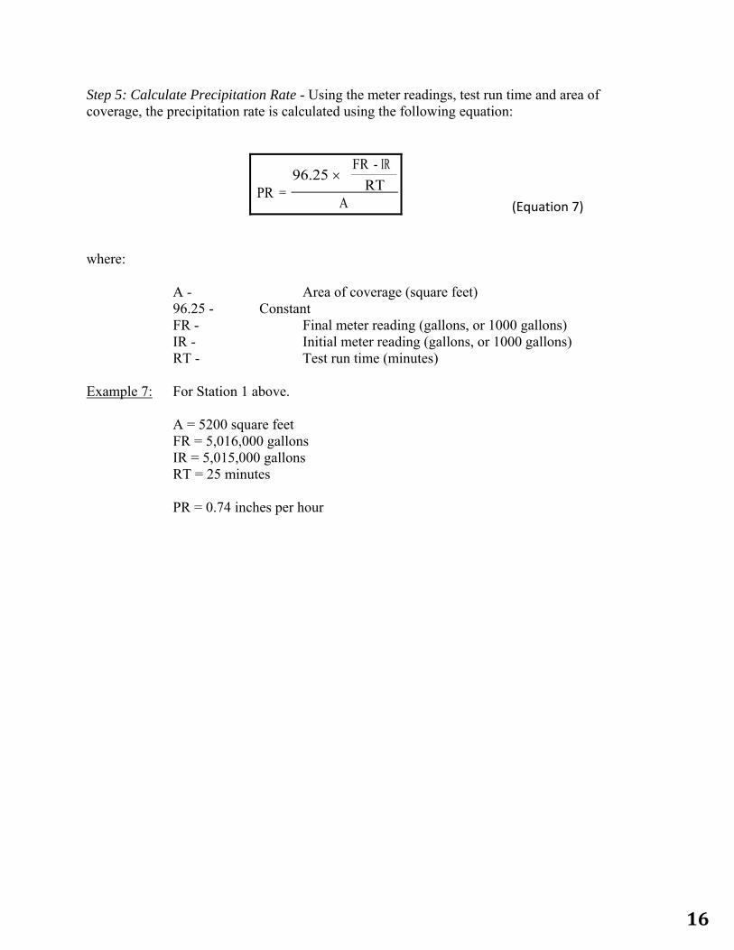
Step 5: Calculate Precipitation Rate - Using the meter readings, test run time and area of coverage, the precipitation rate is calculated using the following equation:
PR =
96.25 FR - IR
RTA
(Equation 7) where:
A - Area of coverage (square feet) 96.25 - Constant FR - Final meter reading (gallons, or 1000 gallons) IR - Initial meter reading (gallons, or 1000 gallons) RT - Test run time (minutes)
Example 7: For Station 1 above.
A = 5200 square feet FR = 5,016,000 gallons IR = 5,015,000 gallons RT = 25 minutes
PR = 0.74 inches per hour
16

ADDITIONAL EXAMPLE PROBLEMS Example 1: Calculating Turf Water Requirement (inches)
A bermudagrass turf growing in Brownsville has a crop coefficient of 0.6 and an adjustment factor of 0.8. What is the monthly water requirement for this turf in July?
(Equation 1)
ETo = 7.59 in per month (from Appendix A) Kc = 0.6
Af = 0.8
WR in month 7 59 0 6 0 8. / . .
WR = 3.64 inches for the month of July Example 2: Calculating Plant Available Water (inches)
A bermudagrass turf has an effective root zone depth of 4 inches and is growing in a loam soil. If the managed allowable depletion is 50%, how much water is available to the turf?
(Equation 2)
D = 0.33 feet, (4 inches ÷ 12 inches per foot) SWHC = 1.7 inches per foot (from Table 1, page 5) MAD = 0.50
PAW ft in ft 0 33 1 7 0 5. . / .
PAW = 0.28 inches
PAW = D SWHC MAD
WR = ET K Ao c f
17

Example 3: Calculating Irrigation Frequency (irrigations per week)
The weekly water requirement for a St. Augustine grass is 1 inch per week. If the plant available water is 0.25 inches, how many irrigations per week are recommended?
(Equation 3)
WR = 1 inch per week PAW = 0.25 inches
I
in week
inches
1
0 25
/
.
I = 4 Irrigations per week
Example 4: Calculating Station Run Time (minutes)
The weekly water requirement for a baseball field is 1 inch per week. The field is irrigated 3 days per week. If Station 1 on the irrigation system has a precipitation rate of 0.5 inches per hour, how long (in minutes) must the station run per irrigation?
(Equation 4)
WR = 1 inch I = 3 PR = 0.5 inches per hour
RT
inch
in hourhour
1
3 0 560
. /min/
RT = 40 minutes
IWR
PAW
RT =WR
I x PR x 60
18
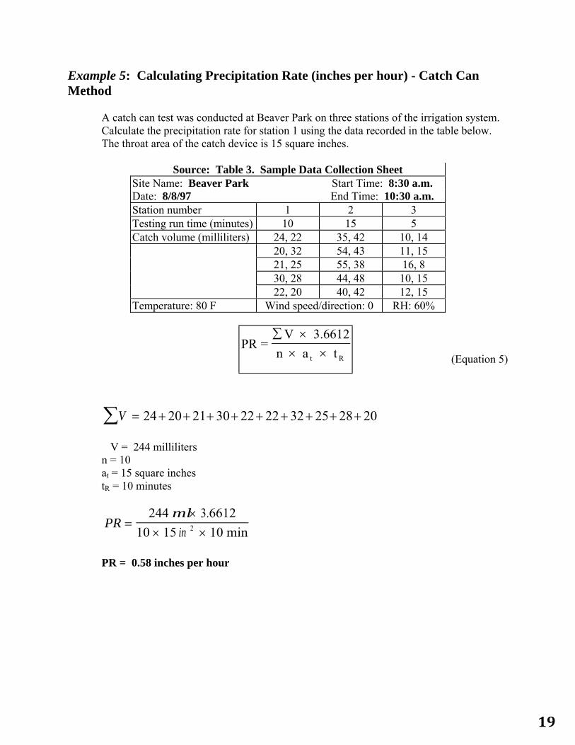
Example 5: Calculating Precipitation Rate (inches per hour) - Catch Can Method
A catch can test was conducted at Beaver Park on three stations of the irrigation system. Calculate the precipitation rate for station 1 using the data recorded in the table below. The throat area of the catch device is 15 square inches.
Source: Table 3. Sample Data Collection Sheet
Site Name: Beaver Park Start Time: 8:30 a.m. Date: 8/8/97 End Time: 10:30 a.m. Station number 1 2 3 Testing run time (minutes) 10 15 5 Catch volume (milliliters) 24, 22 35, 42 10, 14 20, 32 54, 43 11, 15 21, 25 55, 38 16, 8 30, 28 44, 48 10, 15 22, 20 40, 42 12, 15 Temperature: 80 F Wind speed/direction: 0 RH: 60%
(Equation 5)
V 24 20 21 30 22 22 32 25 28 20
�V = 244 milliliters n = 10 at = 15 square inches tR = 10 minutes
PR
ml
in
244 3 6612
10 15 102
.
min
PR = 0.58 inches per hour
PR =V 3.6612
n a tt R
19

Example 6: Calculating Precipitation Rate (inches per hour) - Area/Flow Method Calculate the precipitation rate for Station 1 using the Area/Flow method.
(Equation 6)
GPM 4 1 5 6 3 0 2 6 0. . .
GPM = 36 gallons per minute
A ft ft 80 50 A = 4000 square feet
PR
GPM
ft
96 25 36
4000 2
.
PR = 0.87 inches per hour
Station 1
Q Q
H
H
Q
H
FH
H
Q
F
H
SidewalkSprinkler Head
Q Quarter Circle (1.5 GPM)
F
Half Circle (3GPM)
Full Circle (6 GPM)
H
50 feet
80 feet
PR =96.25 GPM
A
20

Example 7: Calculating Precipitation Rate (inches per hour) - Meter Method
Calculate the precipitation rate for Station 1 using data collected below.
Site Name: Park Place Date: 10/20/98 Station number: 1 2 3 Test run time (minutes) 15 15 20 Initial reading (1000 gallons)
0525 0527 0529
Final reading (1000 gallons)
0527 0529 0531
Landscape Area (square feet)
18,000 8,500 10,000
(Equation 7)
FR = 527,000 gallons (527 x 1000) IR = 525,000 gallons (525 x 1000) RT = 15 minutes A = 7000 square feet
PR
gal
ft
96 25
527 000 525 000
15
18000 2
., ,
min
PR = 0.71 inches per hour
PR =96.25
FR- IRRT
A
21


Appendix B ETo and Rainfall Data


