land-use classiﬁcation using taxi gps tracesgpan/publication/2013-tits-land-use.pdf · land-use...

IEEE TRANSACTIONS ON INTELLIGENT TRANSPORTATION SYSTEMS, VOL. 14, NO. 1, MARCH 2013 113

Land-Use Classification Using Taxi GPS TracesGang Pan, Guande Qi, Zhaohui Wu, Daqing Zhang, and Shijian Li, Member, IEEE

Abstract—Detailed land use, which is difficult to obtain, is anintegral part of urban planning. Currently, GPS traces of vehiclesare becoming readily available. It conveys human mobility andactivity information, which can be closely related to the land useof a region. This paper discusses the potential use of taxi tracesfor urban land-use classification, particularly for recognizing thesocial function of urban land by using one year’s trace datafrom 4000 taxis. First, we found that pick-up/set-down dynamics,extracted from taxi traces, exhibited clear patterns correspondingto the land-use classes of these regions. Second, with six featuresdesigned to characterize the pick-up/set-down pattern, land-useclasses of regions could be recognized. Classification results usingthe best combination of features achieved a recognition accuracyof 95%. Third, the classification results also highlighted regionsthat changed land-use class from one to another, and such land-useclass transition dynamics of regions revealed unusual real-worldsocial events. Moreover, the pick-up/set-down dynamics couldfurther reflect to what extent each region is used as a certain class.

Index Terms—Land-use classification, region activeness, socialfunction, taxi traces.

I. INTRODUCTION

LAND-USE classification is an important aspect of urbanplanning. It is defined as the recognized human use of land

in a city. The granularity of land area in land-use classificationranges from buildings to administrative zones. The concept ofland use has been evolving for tens of years from ecologicalvegetation to urban land use and from coarse classes to de-tailed classes. Early research [1], [2] on land-use classificationattempted to recognize different ecological vegetation such asforests and wetlands. Such land-use classification has broadapplications in ecology, studies on the relationship betweenurbanization and deforestation [3], and farmland changes [4].Later studies [5], [6] classified urban land into built-up andnon-built-up lands to delineate urban region and model urbangrowth. Built-up regions were extracted to identify the impactsof urban growth in a spatial context and detect urban land-cover changes with respect to urbanization [7]–[9]. More de-

Manuscript received February 4, 2012; revised May 14, 2012; acceptedJune 19, 2012. Date of publication August 13, 2012; date of current versionFebruary 25, 2013. This work was supported in part by the Qianjiang TalentProgram under Grant 2011R10078, the Zhejiang Provincial Natural ScienceFoundation under Grant Y1090690, and the Fundamental Research Funds forthe Central Universities. The Associate Editor for this paper was X. Zhang.

G. Pan, G. Qi, Z. Wu, and S. Li (Corresponding author) are with the Collegeof Computer Science and Technology, Zhejiang University, Hangzhou 310027,China (e-mail: [email protected]; [email protected]; [email protected];[email protected]).

D. Zhang is with the Department of Telecommunication Network andServices, Institut TELECOM & Maga. SudParis, 91011 Evry Cedex, France(e-mail: [email protected]).

Color versions of one or more of the figures in this paper are available onlineat http://ieeexplore.ieee.org.

Digital Object Identifier 10.1109/TITS.2012.2209201

tailed classification of urban regions has usually focused onland-covers [10]–[12] such as water, railway, and green lands.Most of the studies gave a coarse definition for the regions’social function, namely, residential or nonresidential regions[13]–[17]. Residential regions are critical because residentialchange in area and density is thought to be directly relatedto urbanization [18]. Residential regions can be categorizedinto different density levels [19]–[21] and used to producepopulation statistics [22].

Most urban land-use classification research has used remote-sensing data, particularly satellite images. The first satel-lite (Landsat-1) for monitoring the Earth’s surface waslaunched by NASA in 1972 with resolution of 79 m. Thesatellite resolution increased gradually. After 1999, severalvery high resolution satellites (IKONOS, QuickBird, andOrbView-3) with resolutions of nearly 1 m were launched.The increase of satellite resolution promoted the develop-ment of new land-use classification methods and led tobetter classification results [15], [23], since there was moreeffective context information available from satellite images.Early land-use classification algorithms relied on the moreor less direct relationship between spectral reflectance andthe nature of the materials covering the Earth’s surface [1],[2]. It was observed that such pixel-based classification gotthe worse result when the satellite resolution increased [24],because pixel-based methods did not consider spatial con-text such as local variance in images [25]. Kernel methodsconsider information of all pixels within a moving windowwith a given size and achieve more accurate classificationresults [19], [26]. However, both pixel- and kernel-based tech-niques need to define artificial image structures, such as pix-els and a moving kernel window, whereas actual objects andregions may be irregularly shaped [27]. Object-based clas-sification method is based on the analysis of automaticallysegmented objects from satellite images and is thus viewedto provide a critical bridge between real-world buildings/regions and their radiometric characteristics in Earth observa-tion data [28].

Although different classifications of land use have beenproposed with different objectives and applications, there arevery few works classifying land use based on social functions.In this paper, instead of using remote-sensing techniques, weattempt to exploit large-scale real-world taxi data to reveal thesocial function of a certain urban area. Concretely, we firstuse clustering techniques to partition the city map into variousareas (zones). Second, we verify that the social function of acertain urban area can be characterized by the temporal andspatial dynamics of the taxi pick-up/set-down number. Third,we use real-time taxi data to predict the social function of a testurban area. Finally, based on the inferred social function of the

1524-9050/$31.00 © 2012 IEEE

114 IEEE TRANSACTIONS ON INTELLIGENT TRANSPORTATION SYSTEMS, VOL. 14, NO. 1, MARCH 2013

test area and context information such as traffic flow densityor historic function change, we characterize the activeness ofthe area corresponding to its social function and track the areafunction transition.

Based on the preceding steps, the main contributions of thispaper are as follows:

1) We defined a new problem and a new way for land-useclassification. Previous land-use classification researchwas based on the physical properties of studied objectsin remote-sensing data. Classification on social function(used as a synonym for land-use class in this paper) ofregions was coarsely defined as residential or nonresiden-tial. We defined the regions’ land-use classes accordingto their social function and similar to map legends. Ournew method for land-use classification is based on pas-senger pick-up/set-down dynamics extracted from real-world taxi trace data. In this paper, such pick-up/set-downdynamics simply describe the variation of pick-up/set-down number over time.

2) We observed and verified that there is an inherent re-lationship between land-use classes and the temporalpattern of taxi pick-up/set-down dynamics. We found thatregions with different land-use classes exhibited differentpick-up/set-down dynamic patterns. For example, scenicspots have more passengers in daytime than at nightand have more passengers during holidays rather thanweekdays.

3) We used verified relationship to identify the social func-tion of urban area. According to the verified relationship,we designed six features extracted from the pick-up/set-down data of different time lengths. Each of thefeatures was evaluated to recognize the regions’ socialfunction for different classifications. The best combina-tion of features achieves a recognition accuracy of 95%using a support vector machine (SVM) classifier.

4) We could inform the transition in terms of its social func-tion and the activeness of urban area by using passengerpick-up/set-down dynamics. We find that social functionof regions is not steady all the time; some regions changefrom one social function to another. Our classificationresult could find social function transition of regions, andsuch transitions are proved to correspond to real-worldunusual social events. Activeness measures to what extenta region is used for its social function. In this paper,human flow characteristics are adopted to depict regionactiveness. As samples of human flow, our passengerpick-up/set-down dynamics directly reflects the active-ness of all kinds of regions.

The remainder of this paper is organized as follows.Section II reviews related works on land-use classification andtaxi trace data. Section III introduces our city-scale taxi tracedata and the extraction of pick-up/set-down number. We alsodiscuss the characteristics of distribution of passenger pick-up/set-down number in this section. In Section IV, we extractregions from the pick-up/set-down data with a refinementof the density-based spatial clustering of applications withnoise (DBSCAN) clustering algorithm. Features are designed

to characterize the regions’ passenger pick-up/set-down dy-namics and then classified in Section V. In Section VI, weshow, using pick-up/set-down dynamics, the region activenessand the social function transition. Section VII concludes thispaper.

II. RELATED WORKS

This section briefly reviews related works on taxi trace dataand urban land-use classification.

Ubiquitous mobility data contain information that is impor-tant for the smart environment [29], [30]. In particular, taxitrace data reflect urban traffic behaviors and convey lots ofinformation about a city. Taxi trace data could be used for:1) rebuilding a city road map [31]; 2) providing informationabout traffic conditions [32], analyzing potential traffic hotspots[33], and detecting flawed urban planning [34]; 3) indentifyingroutes for navigation since taxi trace data imply the experiencedtaxi drivers’ knowledge about the temporal and spatial trafficconditions. It could be used for driving route recommendationsand helping people avoid traffic jams [35], [36]; 4) providinga driving strategy because experienced taxi drivers also havestrategies for hunting or waiting for the next passenger. Thesestrategies could be recommended specifically for taxi driversto find more passengers [37], [38]; and 5) determining anabnormal trajectory since some taxi drivers may be intention-ally choosing a longer route to make more of a profit. Suchabnormal behaviors could be detected using taxi trace data[39]. Other mobility data may also contain information [40],[41], that can be used for developing intelligent transportationsystems [42]–[44].

Previous works on urban land-use classification usually em-ploy remote-sensing techniques. They differ from this paper intwo ways. First, few works considered fine-grained classifica-tion of urban social function. Aubrecht et al. [45] used manyclasses of the regions’ social function to build a city model,while they did not give any approach to classifying urban landuse. Some of the previous research [46]–[48] focused on land-cover classification of two kinds of social function, namely,residential and nonresidential [12], [20]. Some work [16], [49]also defined roads (like highway, railway, and so on) as land-use classes. Herold et al. [27] studied three classes of socialfunction: 1) residential; 2) commercial and industrial; and3) institution. Van de Voorde et al. [17] defined four classes:1) commercial; 2) industrial; 3) service; and 4) residential. Allof these definitions of urban land-use classes are based on visualdifferences among urban regions. None of the previous workprovided a fine-grained classification of the regions’ socialfunction as this paper does, since remote-sensing data cannotdepict enough information.

Second, few works can handle the social activeness of allkinds of regions. Social activeness measures the extent to whicha region is used for its social function. Previous work depictedthe activeness information by visual analysis of building densityfrom remote-sensing images, for example, density level for resi-dential regions [15], [17], [20] and density level for commercialdistricts [14]. This kind of approach has two limits: 1) Visualanalysis of building density is not suitable for the building-scale

PAN et al.: LAND-USE CLASSIFICATION USING TAXI GPS TRACES 115

regions, although it may be fine for regions consisting of lots ofbuildings. 2) It did not depict the activeness of human socialactivities since building density is not closely related to humanmobility.

There are quite a few approaches using mobility data forland-use classification in the literature. The first work on land-use classification using mobility data is our previous work [50],of which this paper is an extension. The main differences arethe following: 1) a new clustering algorithm is introduced;2) the land-use classification approach is redesigned for moreland-use classes and is more effective; 3) social activenessis presented; and 4) we further investigate the problem andcarry out extensive experiments. Recently, Soto and Frias-Martinez [51] reported work on the clustering regions’ landuse using cell phone data. However, they could only getvery large zones and did not present any quantitative classi-fication results. Also, Zhang et al. explored the relationshipbetween origin–destination (OD) flows and social functionof origins and destinations to mine the semantics of ODflows [52].

III. CHARACTERISTICS OF TAXI GLOBAL POSITIONING

SATELLITE TRACE DATA SET

A. Data Set Description

The taxi GPS trace data set used in this paper comes fromthe Hangzhou City Traffic Bureau. Hangzhou, located in thesoutheast region of China, is the capital of Zhejiang provinceand one of the most famous tourist cities in China. The taxi GPStraces were generated over a period of 385 days (from April1, 2009 to April 20, 2010). During this period, the number oftaxis installed with a GPS device increased from 4597 to 7475,whereas the total number of taxis in the city remained almostunchanged. The data set contains approximately three billionrecords; most of them were sampled at a frequency of about1 min. Each record consists of the following information:

1) TAXI ID: the unique ID of each taxi;2) TIME: the sample timestamp “YYYY-MM-DD HH:MM:

SS”;3) GPS POSITION: the current longitude and latitude;4) SPEED: the current taxi speed in km/h;5) TAXI ORIENTATION: the direction the taxi is heading

in, from 0◦ to 360◦ in clockwise (North is 0◦);6) GPS STATE: it is set to 1 if the GPS data is incorrect,

and 0 otherwise. In our experiment, all the records withincorrect GPS data are removed.

7) METER STATE: it indicates whether the taxi meter isrunning, i.e., whether the taxi is occupied.

B. Extraction of Pick-Up/Set-Down Number

The pick-up/set-down number of passengers in a region isimportant for depicting the characteristics of human mobility.It characterizes passengers that come to (or leave) this regionduring a given period. Such mobility information may berelated to the properties of the region and reflects the land-use(social function) classes of the region. The number of pick-up/

Fig. 1. Heatmap of pick-up numbers in a local area near the HangzhouRailway Station. The color bar on the right side illustrates different colors fordifferent pick-up numbers.

set-down events is extracted from the mass of taxi traces withthe following two steps:

1) Sampling: 4000 taxis were sampled randomly each day,and their traces were retrieved for further analysis, tosolve the problem that the number of taxis that installGPS devices does not remain constant in the observedyear.

2) Extracting Pick-up/Set-down Events: Transition of themeter state reflects that passengers are picked up or setdown. More specifically, a pick-up (set-down) event wasextracted from taxi traces when the meter state changesfrom 0 (1) to 1 (0).

C. Distribution of Pick-Up/Set-Down Number

Here, we explore the distribution of pick-up/set-down num-bers over the city. Based on the statistics of the pick-upnumber in a week (from April 1, 2009 to April 7, 2009) foreach small block (10 × 10 m2) of the city, we observed thefollowing:

1) Sparsity of pick-ups: Only a few blocks have a coupleof passengers picked up, and most of the blocks havevery few pick-ups. There are 98.82% of blocks havingno passenger picked up; 0.66% of blocks have just onepick-up; and there are only 0.14% of blocks with morethan 16 pick-ups in the week.

2) Clustering phenomenon: Blocks with passengers pickedup frequently usually cluster with each other, which yieldmany clusters of high pick-up density within the city.Fig. 1 shows the pick-up number heatmap of a local areanear the Hangzhou Railway Station, where the clusteringphenomenon is obvious.

3) Disparity of clusters: The clusters formed by blocks withmany pick-ups are different in pick-up density and clustersize. As an example, we simply generate the clusters bymerging blocks with more than 16 passengers in a four-connected manner, and the pick-up histogram is shown inFig. 2. The pick-up density is in a wide range, and thecluster count drops quickly with the increase of pick-upnumber. Moreover, the clusters have different sizes; the


Fig. 2. Pick-up density histogram. Clusters are simply obtained by mergingthe blocks with more than 16 pick-ups.

largest cluster contains 452 blocks, whereas the smallestclusters contain only one block.

The three properties of pick-up distribution provide insightsfor the extraction of regions. First, we focus on blocks withmany pick-ups since blocks with few pick-ups contain littleinformation of human mobility. The first property shows thatthere are very few blocks with many pick-ups. Second, suchblocks, according to the second property, yield many regularclusters. Such regular clusters are rough approximations toreal-world irregular regions. In this paper, these regions areextracted with clustering methods. Third, the difference of pick-up density and size among clusters makes region extractionmore challenging. Some adaptive mechanism is required toachieve an effective region extraction.

IV. REGION EXTRACTION: DBSCAN-BASED CLUSTERING

Regions with high pick-up density are informative in con-veying human mobility cues, which is related to the socialfunction of regions. This paper focuses on regions with highpick-up density. From the algorithmic view, these regions canbe defined as convex hulls of clusters within the set of pick-up/set-down points. The challenge of extracting clusters comesfrom the disparity of clusters. We refine the traditionalDBSCAN clustering algorithm [53] to solve this problem.

A. Terminology and Notations

For facilitating further description, several definitions andterms are listed below, which are much similar to the DBSCANalgorithm [53]

Definition 1: The point set to be clustered is S, S = {p :p = (x, y)}, where p represents any pick-up position, x is thelongitude, and y is the latitude of p.

Definition 2: The d-neighborhood of a point p is denotedby Nd(p) = {q : q ∈ S,L2(p, q) < d}, where L2(p, q) is theEuclidean distance between p and q.

Definition 3—Average Neighbor Number: The averageneighbor number of points in a point set R is denoted as

averd(R) =

∑|Nd(p)||R| , p ∈ R.

Definition 4—Directly Density Reachable: p is directly den-sity reachable from a point q with respect to MinPts and d ifand only if p ∈ Nd(q) and |Nd(q)| ≥ MinPts.

Definition 5—Density Reachable: p is density reachablefrom a point q with respect to MinPts and d if there existsa chain of points p1 = p, p2, . . . , pn = q, where pi is directlydensity reachable from pi+1 for i = 1, . . . , n− 1.

Definition 6—Cluster: A cluster C with respect to MinPtsand d is a nonempty subset of S satisfying the following. 1) ∀ p,q, if q ∈ C and p is density reachable from q with respect to dand MinPts, then p ∈ C; 2) ∀ p, q ∈ C, ∃o ∈ C, so that bothp and q can be density reachable from o with respect to d andMinPts.

Definition 7—Convex Hull and Area: Define a convex hullof a cluster of points C as P = conv(C). This convex hull is apolygon; its area is denoted as area(P ).

Definition 8—Polygon Distance: Define the distance be-tween two polygons Pi and Pj as distp(Pi, Pj) = min(L2(pi,pj)), where pi is any point located in Pi, and pj is any pointlocated in Pj .

B. IDBSCAN: Iterative DBSCAN Clustering Algorithm

DBSCAN is a widely used density-based clusteringalgorithm. It is simple and thus efficient for large-scale data.However, the original DBSCAN algorithm essentially fixes aunique density threshold for all the clusters. It is not effectivefor extracting clusters with different pick-up/set-down density.Thus, we refine the DBSCAN algorithm by adaptively settingthe density threshold of clusters and iteratively extractingthem with reasonable size. The refined algorithm is named asIDBSCAN.

Given the point set S and d, our IDBSCAN algorithm re-trieves the final cluster set as follows:

Algorithm: Iterative DBSCAN

1: Initialize: SC = {S}; Ab = 10000 m2

2: While ∃C ∈ SC , s.t. Area(conv(C)) > Ab

3: SL = C;4: if SL ⊂ S, MinPts = averd(SL);5: for all p ∈ SL:6: Sp = {p}, SL = SL \ Sp;7: While ∃q ∈ Sp, s.t. |Nd(q)| ≥ MinPts and SL ∩

Nd(q) = ∅8: Sp = Sp ∪Nd(q), SL = SL \Nd(q);9: end While

10: SC = SC ∪ {Sp};11: end for12: SC = SC \ {C};13: end While

Steps 3–12 (the inner loop) is the original DBSCAN algo-rithm. The previous definition of clusters provides a direct wayto divide all points into clusters. If started from an in-classpoint p, all the point densities reachable from p will be put inthe cluster that p belongs to. By setting MinPts and d, the


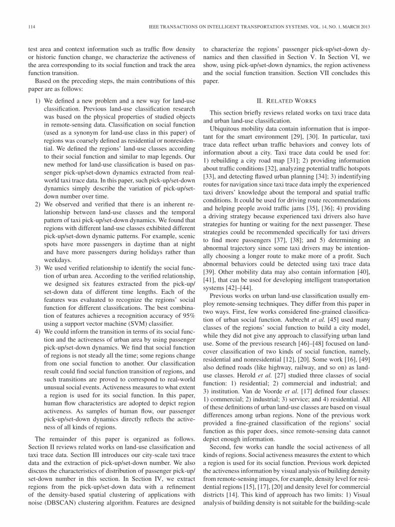
Fig. 3. Comparison of IDBSCAN and DBSCAN in four cases. (a) Two clusters with similar density separated with each other very well. (b) Two clusters withdifferent density. (c) Two clusters with similar density are close. (d) Two clusters are overlapped too much. The horizontal lines mean the density threshold forcluster extraction.

DBSCAN algorithm fixes a density threshold and gets the clus-ters above the density threshold. However, for heterogeneousdata, such a unique density threshold may result in clusterswith size varying in a large range. Too large regions may havemultiple social functions, while too small regions will have fewpassengers.

The outer loop is our refinement of the original DBSCANalgorithm. The refinement could segment a large cluster intosmaller clusters with higher pick-up density since the refine-ment repeatedly runs DBSCAN on clusters larger than a boundsize with increasing density threshold. Such refinement pre-vents getting very small clusters since it begins with largeclusters (gotten with an initial low density threshold) and thendecreases in size gradually. It also prevents getting very largeclusters because the area is restricted with an upper bound. Ac-cording to our observation on the taxi trace data of Hangzhou,this bound is empirically set to be large (100 × 100 m2).

C. Evaluation

We illustrate 4 typical cases to demonstrate the advantageof IDBSCAN compared with DBSCAN, shown in Fig. 3. Forthe first case shown in Fig. 3(a), two clusters with similardensity separated with each other very well; both algorithmsget a good clustering result. For the second case shown inFig. 3(b), the density of the two clusters is very different. TheDBSCAN algorithm gets clusters with very large size, whereasour algorithm can iteratively run the clustering procedure withincreasing density threshold and find clusters with the desiredsize. For the third case, shown in Fig. 3(c), two clusters stayclose, and DBSCAN cannot separate them. However, if thetotal area of the two clusters is larger than the area bound, ouralgorithm can separate them. If the two clusters lie very closelyand the total area is small, then our algorithm may also fail,

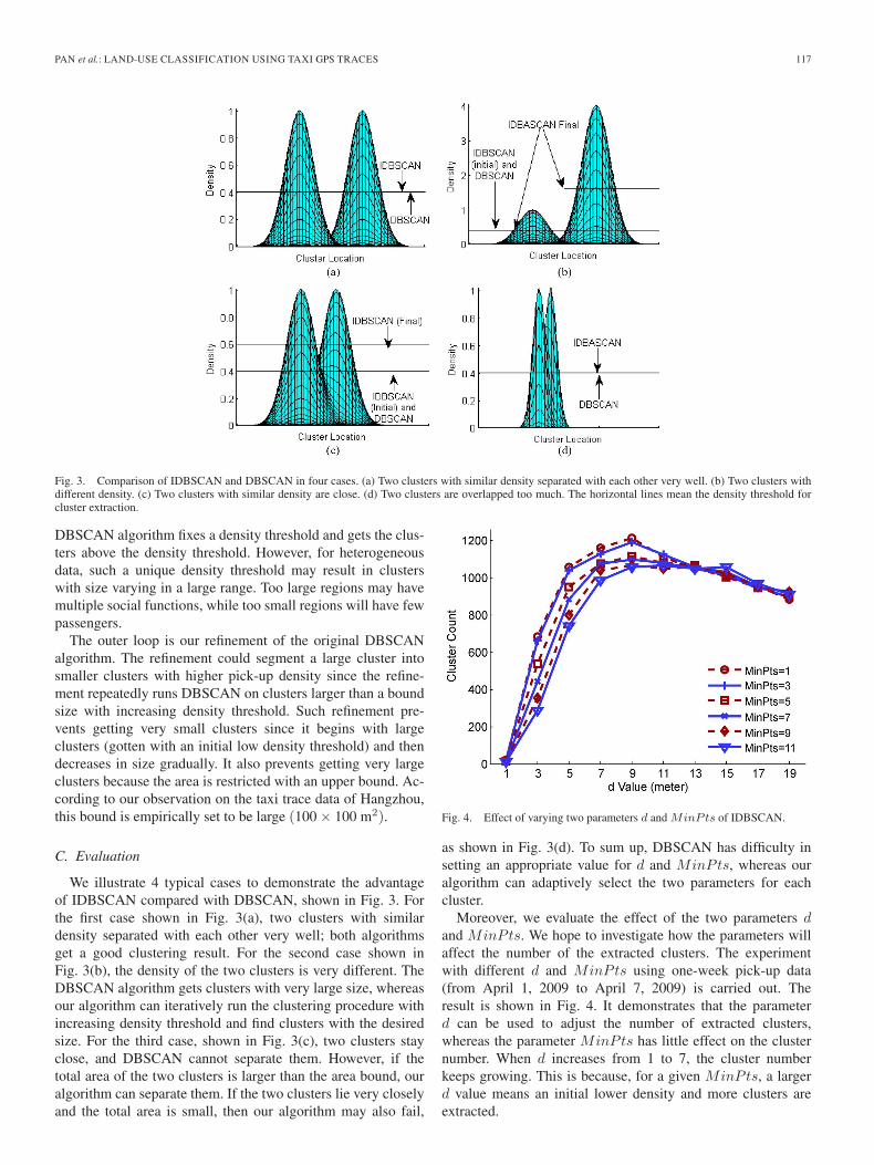
Fig. 4. Effect of varying two parameters d and MinPts of IDBSCAN.

as shown in Fig. 3(d). To sum up, DBSCAN has difficulty insetting an appropriate value for d and MinPts, whereas ouralgorithm can adaptively select the two parameters for eachcluster.

Moreover, we evaluate the effect of the two parameters dand MinPts. We hope to investigate how the parameters willaffect the number of the extracted clusters. The experimentwith different d and MinPts using one-week pick-up data(from April 1, 2009 to April 7, 2009) is carried out. Theresult is shown in Fig. 4. It demonstrates that the parameterd can be used to adjust the number of extracted clusters,whereas the parameter MinPts has little effect on the clusternumber. When d increases from 1 to 7, the cluster numberkeeps growing. This is because, for a given MinPts, a largerd value means an initial lower density and more clusters areextracted.


TABLE ISTATISTICS OF THE EXTRACTED REGIONS

However, the cluster number decreases a little when d in-creases from 7 to 9, which is caused by those clusters closeto each other. When d is small, these clusters will be extractedseparately; when d is too large, these clusters merge into a largercluster.

D. Result of Region Extraction

We use the IDBSCAN algorithm to extract clusters fromthe taxi GPS trace data described in Section III. The param-eter setting is as follows: d = 5, and MinPts = 5. There are952 regions extracted. However, the social function of theseregions is still unknown. To build a data set with socialfunction for study, we employ the manual labeling strategy.Six experienced taxi drivers were invited to label the socialfunction for the extracted regions. They were asked to la-bel only those regions with relatively single (or pure) so-cial function. We ended up with 534 regions with a labeledsocial function. These regions belong to eight kinds of so-cial function, i.e., coach/train station, campus, hospital, scenicspot, commercial district, entertainment district, office build-ing, and residential district. The data demography is listed inTable I.

V. LAND-USE CLASSIFICATION

The pick-up/set-down dynamics is to describe the variationof pick-up/set-down number over time. First, we reveal theinherent relation between land-use classes and temporal pat-terns of pick-up/set-down dynamics. Second, to evaluate howuseful the pick-up/set-down dynamics would be for land-useclassification, six features are designed. Four typical classi-fiers are then employed to recognize the social function (landuse) of regions. Moreover, we explore which features whencombined could achieve the optimal classification performance.Moreover, we evaluate how much time of historical data thefeature extraction requires to obtain reasonable classificationaccuracy.

A. Definitions and Terminology

For a region R, in this paper, the pick-up/set-down dynam-ics is defined as a temporal sequence consisting of pick-up/set-down numbers in the time interval of an hour. Thus, thedynamics of a day can be denoted by a 24-dimensional vector.In the case of many days, it can be denoted by a dynamicsmatrix, each of whose columns is for one day.

For convenience in further discussion, we give the terminolo-gies and definitions as follows:U the pick-up dynamics matrix of a region;D the set-down dynamics matrix of a region;aj,k an element of the dynamics matrix A, describing the

pick-up/set-down number within the jth hour of thekth day;

aj,: row vector of matrix A;a:,k column vector of matrix A;Sh day set of holidays;|S| cardinality of the set S;‖v‖ L2 norm of the vector v;N(v) normalization of a vector v, denoted as N(v) =

(v/‖v‖);u./v element-wise division of two vectors u and v.

B. Relationship Between Land Use and Passenger Dynamics

Fig. 5 plots the daily pick-up pattern for four kinds of regionland use as examples. The daily pick-up pattern shows the meanpick-up number in each hour of a day averaged over a yearfor each region. Meanwhile, the standard variance of the pick-up number among the same kind of regions is plotted in thincolor shadow. We explicitly separate weekdays and holidays.The figure shows that different land-use classes differ greatly inpeak value, daily fluctuation, and weekday–holiday disparity.

C. Feature Extraction

A good feature will very much help the land-use clas-sification of a region. This paper designs and investigates6 pick-up/set-down features, which are extracted from thepick-up/set-down dynamics matrix U/D, to explicitly depictthe characteristics of a region R. All the features are computedusing the historical data of a certain time length, for example,three-month taxi GPS data.

1) Daily pick-up feature (I): The daily pick-up feature pro-vides information about the pick-up number in eachhour of a day. The feature can be denoted as a48-dimensional vector, composed of the holiday part(24 dimensions) and the weekday part (24 dimensions).The holiday part for the region R is calculated as

vIh =

∑k∈Sh

N(u:,k)

|Sh|

and the weekday part is computed similarly.2) Daily set-down feature (II): Similar to the daily pick-

up feature, this feature is the set-down number per houraveraged over days, with holidays and weekdays, respec-tively. It also has 48 dimensions.

3) Pick-up/set-down difference feature (III): It representsthe difference of the pick-up number and the set-downnumber in each hour. It is denoted as a 48-day vectorcomposed by the holiday part and the weekday part; theholiday part is obtained by

vIIIh =

∑k∈Sh

(N(u:,k)−N(d:,k))

|Sh|.


Fig. 5. Daily pick-up pattern (in line) for four classes of regions along with their standard variance (in shadow). (a) Station. (b) Scenic Spot. (c) CommercialDistrict. (d) Entertainment District.

Fig. 6. Classification results of six features and four algorithms. I, II, III, IV, V, and VI indicate the different kinds of features. Four different lengths of data forfeature extraction are tested (a) One year. (b) Half a year. (c) Four months. (d) One month.

4) Pick-up/set-down ratio feature (IV): It measures the ratioof the pick-up number to the set-down number in eachhour of a day. Its holiday part is calculated as

vIVh =

∑k∈Sh

(N(u:,k)./N(d:,k))

|Sh|.

5) Weekly pick-up feature (V): The weekly pick-up featurefor a region R depicts the variation of pick-up number ofeach day in a week. It is a 7-dimension vector calculatedas

vVi = C

⎛⎝∑

j

∑k

uj,7k+i

⎞⎠ , i = 1, 2, . . . , 7, k ≥ 0

where C is the factor for normalizing the vector.6) Weekly set-down feature (VI): vVI

i =CN (

∑j

∑k dj,7k+i), i = 1, 2, . . . , 7, k ≥ 0.

D. Experiments

We test the land-use classification performance using534 regions with eight kinds of social functions (land use):1) station; 2) campus; 3) hospital; 4) scenic spot; 5) commer-cial district; 6) entertainment district; 7) office building; and8) residential district. The data demography is shown in Table I.They are extracted from the nearly one-year real-world taxitrace data of Hangzhou City, and the associated social functionis labeled by six professional taxi drivers.

Four classical classifiers are evaluated for land-use classifi-cation. They are linear-kernel SVM, k-nearest neighbor, lineardiscriminate analysis, and three-layer BP (backward propaga-

tion neural network). All the parameters for the algorithms areoptimized.

1) Experimental Setup: We employ the tenfold cross-validation policy. All the regions belonging to the same landuse are randomly divided into ten folds as evenly as possible(the difference between the region number of any two folds isnot larger than one). In each round, nine folds are for trainingclassifiers and the rest for validation. Thus, any region forvalidation will never simultaneously appear in the training setof regions. We repeat this procedure ten times. The advantageof this policy is that all regions are used for both training andvalidation in an interleave way, and each region is used forvalidation exactly once.

The six kinds of features depend on the time length of datafor extraction. The longer time length will let features conveymore land-use information but make them less sensitive totemporal change of land use. In the experiment, given a timelength for feature, we partition the data of each region intoseveral parts of the same time length. Each part of the datais to generate an individual feature vector, which serves as anindependent training or validation sample for evaluation.

2) Experiment 1—Evaluation of Features and Algorithms:This experiment is to evaluate the discriminative capability ofthe six kinds of features and the classification performance ofthe four algorithms. For each kind of feature and each algo-rithm, four different time lengths of data for feature extractionare tested: one year, half a year, four months, and one month.The experiment result is shown in Fig. 6.

As for the discriminative capability of a single feature,feature I is the best among the six features, for almost allfour time lengths and four algorithms. The best performanceachieves 88.62%, with the SVM classifier and 4-mo data forfeature extraction. Features V and VI are the worst ones,


TABLE IIFEATURE SELECTION RESULTS

Fig. 7. Visualization of 3 classes of regions after the dimensionality reductionto 3 with MDS.

whose classification accuracy is generally below 60%. Theresults demonstrate that the daily pick-up/set-down information(features I, II, III, and IV) is very helpful.

As for classifiers, in many cases, SVM performs best inland-use classification for all six features and four time lengthsthanks to its powerful generalization capability. The BP net-work has the lowest accuracy among the four algorithms.

3) Experiment 2—Feature Selection: Different features mayconvey different but complementary information on land use.The feature selection experiment attempts to find the bestcombination of features for classification. The new combinedfeature is generated by concatenating the two to six originalfeature vectors. The best feature combination is selected usingthe forward–backward feature selection algorithm [54] and thebrutal force algorithm, respectively. The forward–backward al-gorithm iteratively executes a forward step and then a backwardstep until convergence. The forward (backward) step repeatedlyadds (deletes) the best (worst) feature unless the classificationaccuracy decreases. The brutal algorithm enumerates all thefeature combinations (26 in total) and finds the best one. Thefour classifiers are all evaluated. We choose the time length of4 mo for feature extraction.

The feature selection result is shown in Table II. For the casesof four classifiers, the two feature selection methods always getthe same feature selection result: feature I + feature II. The twofeature combination achieves the best classification accuracy of95.65% when the SVM classifier is used. This combination iseven better than combining all the features.

To visualize the feature I + II space, we use multidimen-sional scaling (MDS) to reduce the feature to three dimensions

Fig. 8. SVM classification by different features with varying time length forfeature extraction.

and plot all the three classes of social function, residentialdistrict, hospital, and scenic spot in Fig. 7.

4) Experiment 3—Varying Time Length for Feature Extrac-tion: The fewer time length of data for feature extraction, theless cost to build a land-use classifier, while possibly worseclassification accuracy. This experiment is to find how the per-formance changes with the time length for feature extraction.We vary the time length of data from ten days to half a year.The SVM classifier is used.

Fig. 8 shows the experimental results with the SVM classifierby different features. It finds that the accuracy using any featurealways decreases when the time length decreases. The perfor-mance decrease becomes quick when the time length comesbelow 30 days. For the best feature combination (feature I +feature II), the classification performance keeps above 90%when the time length is larger than 30 days, and the best resultis achieved with the time length of 4 mo.

VI. REGION DYNAMICS AND SOCIAL ACTIVENESS

A. Region Dynamics

A region’s social function does not remain consistent all thetime. It may change when buildings in the region are disusedfor reconstruction or change their utilization. For example, theland-use class of a region will change from station to residentialdistrict if the train station in the region is replaced by apartmentbuildings. We call such dynamic change of land use over timeas region dynamics.

The land-use classification result of a region over time canbe used to depict the region dynamics. We employed the timelength of 1 mo for feature extraction and classified land use ofall the regions of each month. We found that the land use ofmany regions changed stably during the period of April 2009 toMarch 2010.

Transition of social function is usually caused by unusualsocial events, such as traffic regulation, building reconstruction,and new center opening. For five transition examples, we fur-ther investigate the underlying social events that cause a changein land use. The social events are listed in Table III. We can seethat regions 2 and 3 changed their land use mainly because ofa building closing, the land-use transition of regions 1 and 5was mainly caused by the opening of new big center, and the


TABLE IIISOCIAL EVENTS BEHIND THE SOCIAL FUNCTION TRANSITION

Fig. 9. Social activeness of some regions. (a) Social activeness variationamong different times in the Xixi wetland. (b) Social activeness of some regionsin the main city zone on April 1, 2009. The color density indicates theiractiveness.

transition of region 4 was due to traffic regulation (not strictlyobeying the prohibition regulation at night makes it change tothe land use of entertainment).

B. Social Activeness

It is usually in a different degree that regions are utilizedfor a social function, depending on time and location. We callthis kind of utilization activeness degree for a region as socialactiveness. It depicts to what extent a region is used for asocial function. The regions with a similar social function aredifferent in social activeness, and a region has different socialactiveness at different times. For example, some scenic spotshave more tourists than others and a certain scenic spot mayhave more passengers in spring than in winter. Such socialactiveness reflects human flow information. It can be exploitedto find popular spots for drivers, tourists, and passengers.

We simply compute the social activeness of a region as thetotal pick-up number of a day. The results with the pick-up datafrom April 1, 2009 to March 31, 2010 show the following:

1) Temporal variation of social activeness. The social ac-tiveness of a region may vary in different days. Fig. 9(a)

illustrates a famous scenic spot, the Xixi wetland, duringdifferent days. The Xixi wetland has peaks in the springand during October, because people like to go for holi-days in warm seasons (e.g., spring plus October).

2) Spatial variation of social activeness. Social activenessalso varies spatially, different in regions at the same time.As an example, Fig. 9(b) shows the social activeness ofsome regions in the main city zone on April 1, 2009. So-cial activeness of regions is described in color density. Inthis figure, the regions within red circle are more sociallyactive than the other regions. This is because it is the com-mercial area of the city with lots of large shopping malls.

VII. CONCLUSION AND DISCUSSIONS

In this paper, we explore and prove the potential use oftaxi trace data in land-use classification. The data used in thispaper are large-scale real-world taxi trace data of a big citywith a population of 6 million. First, an improved clusteringalgorithm (iterative DBSCAN) is presented to extract regions,according to the characteristics of the data. Second, the land-useclassification using the taxi trace data is proposed. Six kinds offeatures are designed, and four classifiers are integrated into theevaluation. The performance of different features and classifiersis evaluated, and a best feature combination is also achieved.With the large-scale data, our approach can achieve an accuracyof 95% for land-use classification. Third, the dynamic transitionof a region’s land use can be detected and reveal correspondingsocial events.

Our work still has some limits for land-use classification.First, we cannot address regions that have few taxi passengers.The taxi passenger flow is only a small part of the wholehuman flow and this results in some regions having fewerpassengers. However, if the trace data of personal cars areavailable, our method can be easily applied to complementarytrace data to handle more regions. Second, our work currentlyonly addresses regions with pure land use. We do not considerregions with multiple land-use classes, which will be focus offuture work.

ACKNOWLEDGMENT

The authors would also like to thank the Hangzhou CityTraffic Bureau for providing the taxi trace data, which becamethe basis for their research. They would also like to thank thesix professional drivers for their manual labeling of land use.


REFERENCES

[1] F. Sadowski and I. Sarno, “Forest classification accuracy as influenced bymultispectral scanner spatial resolution,” Environ. Res. Inst. Michigan,Ann Arbor, MI, Rep. 109600-71-F, 1976.

[2] R. Latty and R. Hoffer, “Computer-based classification accuracy due todata spatial resolution using a per-point vs per field classification tech-niques,” in Proc. Mach. Process. Remotely Sensed Data Symp., 1981,pp. 384–393.

[3] H. Geist and E. Lambin, “What drives tropical deforestation? A meta-analysis of proximate and underlying causes of deforestation based onsubnational case study evidence,” Land Use and Cover Change, Rep. Ser.No. 4, 2001. [Online]. Available: http://www.pik-potsdam.de/members/cramer/teaching/0607/Geist_2001_LUCC_Report.pdf

[4] Y. Xie, Y. Mei, T. Guangjin, and X. Xuerong, “Socio-economic drivingforces of arable land conversion: A case study of Wuxian City, China,”Global Environ. Change, vol. 15, no. 3, pp. 238–252, Oct. 2005.

[5] S. Chen, S. Zeng, and C. Xie, “Remote sensing and GIS for urban growthanalysis in China,” Photogramm. Eng. Remote Sens., vol. 66, no. 5,pp. 593–598, May 2000.

[6] R. Gluch, “Urban growth detection using texture analysis on mergedlandsat TM and SPOT-P data,” Photogramm. Eng. Remote Sens., vol. 68,no. 12, pp. 1283–1288, Dec. 2002.

[7] D. Ward, S. Phinn, and A. Murray, “Monitoring growth in rapidlyurbanizing areas using remotely sensed data,” Prof. Geogr., vol. 52, no. 3,pp. 371–386, 2000.

[8] C. Lo and Y. Xiaojun, “Drivers of land-use/land-cover changes anddynamic modeling for the Atlanta, Georgia metropolitan area,” Pho-togramm. Eng. Remote Sens., vol. 68, no. 10, pp. 1073–1082, Oct. 2002.

[9] W. Ji, J. Ma, R. Twibell, and K. Underhill, “Characterizing urban sprawlusing multi-stage remote sensing images and landscape metrics,” Comput.Environ. Urban Syst., vol. 30, no. 6, pp. 861–879, Nov. 2006.

[10] J. Stuckens, P. Coppin, and M. Bauer, “Integrating contextual informa-tion with per-pixel classification for improved land cover classification,”Remote Sens. Environ., vol. 71, no. 3, pp. 282–296, Mar. 2000.

[11] Y. Zha, J. Gao, and S. Ni, “Use of normalized difference built-up indexin automatically mapping urban areas from TM imagery,” Int. J. RemoteSens., vol. 24, no. 3, pp. 583–594, Feb. 2003.

[12] A. Puissant, J. Hirsch, and C. Weber, “The utility of texture analysis toimprove per-pixel classification for high to very high spatial resolutionimagery,” Int. J. Remote Sens., vol. 26, no. 4, pp. 733–745, Feb. 2005.

[13] P. Gong and P. Howarth, “The use of structural information for im-proving land-cover classification accuracies at the rural-urban fringe,”Photogramm. Eng. Remote Sens., vol. 56, no. 1, pp. 67–73, Jan. 1990.

[14] W. Stefanov, M. Ramsey, and P. Christensen, “Monitoring urban landcover change: An expert system approach to land cover classification ofsemiarid to arid urban centers,” Remote Sens. Environ., vol. 77, no. 2,pp. 173–185, Aug. 2001.

[15] D. Chen, D. Stow, and P. Gong, “Examining the effect of spatial resolutionand texture window size on classification accuracy: An urban environmentcase,” Int. J. Remote Sens., vol. 25, no. 11, pp. 2177–2192, Jun. 2004.

[16] F. Pacifici, M. Chini, and W. Emery, “A neural network approach usingmulti-scale textural metrics from very high-resolution panchromatic im-agery for urban land-use classification,” Remote Sens. Environ., vol. 113,no. 6, pp. 1276–1292, Jun. 2009.

[17] T. Van de Voorde, W. Jacquet, and F. Canters, “Mapping form and functionin urban areas: An approach based on urban metrics and continuousimpervious surface data,” Landsc. Urban Plan., vol. 102, no. 3, pp. 143–155, Sep. 2011.

[18] Y. Weng, “Spatiotemporal changes of landscape pattern in responseto urbanization,” Landsc. Urban Plan., vol. 81, no. 4, pp. 341–353,Jul. 2007.

[19] M. Barnsley and S. Barr, “Inferring urban land use from satellite sensorimages using kernel-based spatial reclassification,” Photogramm. Eng.Remote Sens., vol. 62, no. 8, pp. 949–958, Aug. 1996.

[20] D. Lu and Q. Weng, “Urban classification using full spectral informationof landsat ETM + imagery in Marion County, Indiana,” Photogramm.Eng. Remote Sens., vol. 71, no. 11, pp. 1275–1284, Nov. 2005.

[21] D. Lu and Q. Weng, “Use of impervious surface in urban land-useclassification,” Remote Sens. Environ, vol. 102, no. 1/2, pp. 146–160,May 2006.

[22] J. Jensen and D. Cowen, “Remote sensing of urban/suburban infrastruc-ture and socio-economic attributes,” Photogramm. Eng. Remote Sens.,vol. 65, no. 5, pp. 611–622, May 1999.

[23] G. Wilkinson, “Results and implications of a study of fifteen years ofsatellite image classification experiments,” IEEE Trans. Geosci. RemoteSens., vol. 43, no. 3, pp. 433–440, Mar. 2005.

[24] M. Barnsley, L. Moller-Jensen, and S. Barr, Remote Sensing and UrbanAnalysis. London, U.K.: Taylor & Francis, 2001.

[25] C. Woodcock and A. Strahler, “The factor of scale in remote sensing,”Remote Sens. Environ., vol. 21, no. 3, pp. 311–332, Apr. 1987.

[26] P. Gong and P. Howarth, “Frequency-based contextual classification andgray-level vector reduction for land-use identification,” Photogramm.Eng. Remote Sens., vol. 58, no. 4, pp. 423–437, 1992.

[27] M. Herold, X. Liu, and K. Clarke, “Spatial metrics and image texture formapping urban land use,” Photogramm. Eng. Remote Sens., vol. 69, no. 9,pp. 991–1001, Sep. 2003.

[28] T. Blaschke, “Object based image analysis for remote sensing,” ISPRS J.Photogramm. Remote Sens., vol. 65, no. 1, pp. 2–16, Jan. 2010.

[29] Z. Wu, Q. Wu, H. Cheng, G. Pan, M. Zhao, and J. Sun, “Scud-Ware: A semantic and adaptive middleware platform for smart vehiclespace,” IEEE Trans. Intell. Transp. Syst., vol. 8, no. 1, pp. 121–132,Mar. 2007.

[30] G. Pan, Y. Xu, Z. Wu, S. Li, L. Yang, M. Lin, and Z. Liu, “TaskShadow:Towards seamless task migration across smart environments,” IEEE Intell.Syst., vol. 26, no. 3, pp. 50–57, May/Jun.2011.

[31] L. Cao and J. Krumm, “From GPS traces to a routable road map,” in Proc.ACM GIS, 2009, pp. 3–12.

[32] H. Wang, H. Zou, Y. Yue, and Q. Li, “Visualizing hot spot analysis resultbased on mashup,” in Proc. Int. Workshop Location Based Social Netw.,2009, pp. 45–48.

[33] S. Liu, Y. Liu, L. Ni, J. Fan, and M. Li, “Towards mobility-based cluster-ing,” in Proc. KDD, 2010, pp. 919–928.

[34] Y. Zheng, Y. Liu, J. Yuan, and X. Xie, “Urban computing with taxicabs,”in Proc. 13th Int. Conf. UbiComp., 2011, pp. 89–98.

[35] L. Liu, C. Andris, and C. Ratti, “Uncovering cabdrivers’ behavior pat-terns from their digital traces,” Comput. Environ. Urban., vol. 34, no. 6,pp. 541–548, Nov. 2010.

[36] J. Yuan, Y. Zheng, C. Zhang, W. Xie, X. Xie, G. Sun, and Y. Huang,“T-drive: Driving directions based on taxi trajectories,” in Proc. ACMGIS, 2010, pp. 99–108.

[37] B. Li, D. Zhang, L. Sun, C. Chen, S. Li, G. Qi, and Q. Yang, “Hunting orwaiting? Discovering passenger-finding strategies from a large-scale real-world taxi data set,” in Proc. IEEE Int. Conf. PERCOM Workshops, 2011,pp. 63–68.

[38] X. Li, G. Pan, Z. Wu, G. Qi, S. Li, D. Zhang, W. Zhang, and Z. Wang,“Prediction of urban human mobility using large-scale taxi traces andits application,” J. Frontiers Comput. Sci., vol. 6, no. 1, pp. 111–121,Feb. 2012.

[39] D. Zhang, N. Li, Z. Zhou, C. Chen, L. Sun, and S. Li, “iBAT: Detectinganomalous taxi trajectories from GPS traces,” in Proc. 13th Int. Conf.UbiComp., 2011, pp. 99–108.

[40] F. Calabrese, M. Colonna, P. Lovisolo, D. Parata, and C. Ratti, “Real-timeurban monitoring using cell phones: A case study in Rome,” IEEE Trans.Intell. Transp. Syst., vol. 12, no. 1, pp. 141–151, Mar. 2010.

[41] J. Barria and S. Thajchayapong, “Detection and classification of trafficanomalies using microscopic traffic variables,” IEEE Trans. Intell. Transp.Syst., vol. 12, no. 3, pp. 695–704, Sep. 2011.

[42] F.-Y. Wang, “Agent-based control for networked traffic managementsystems,” IEEE Intell. Syst., vol. 20, no. 5, pp. 92–96, Sep./Oct.2005.

[43] J. Sun, Z. Wu, and G. Pan, “Context-aware smart car: From model toprototype,” J. Zhejiang Univ. Sci. A, vol. 10, no. 7, pp. 1049–1059,2009.

[44] F.-Y. Wang, “Parallel control and management for intelligent transporta-tion systems: Concepts, architectures, and applications,” IEEE Trans.Intell. Transp. Syst., vol. 11, no. 3, pp. 630–638, Sep. 2010.

[45] C. Aubrecht, K. Steinnocher, M. Hollaus, and W. Wagner, “Integratingearth observation and GIScience for high resolution spatial and functionalmodeling of urban land use,” Comput. Environ. Urban Syst., vol. 33, no. 1,pp. 15–25, Jan. 2009.

[46] K. Seto and M. Fragkias, “Quantifying spatiotemporal patterns of urbanland-use change in four cities of China with time series landscape met-rics,” Landsc. Ecol., vol. 20, no. 7, pp. 871–888, Nov. 2005.

[47] A. Carleer and E. Wolff, “Urban land cover multi-level region-basedclassification of VHR data by selecting relevant features,” Int. J. RemoteSens., vol. 27, no. 6, pp. 1035–1051, Mar. 2006.

[48] J. Deng, K. Wang, Y. Hong, and J. Qi, “Spatio-temporal dynamicsand evolution of land use change and landscape pattern in response torapid urbanization,” Landsc. Urban Plan., vol. 92, no. 3/4, pp. 187–198,2009.

[49] M. Luck and J. Wu, “A gradient analysis of urban landscape pattern: Acase study from the Phoenix metropolitan region, Arizona, USA,” Landsc.Ecol., vol. 17, no. 4, pp. 327–339, May 2002.

[50] G. Qi, X. Li, S. Li, G. Pan, Z. Wang, and D. Zhang, “Measuring socialfunctions of city regions from large-scale taxi behaviors,” in Proc. IEEEPERCOM, 2011, pp. 384–388.


[51] V. Soto and E. Frias-Martinez, “Robust land use characterization of urbanlandscapes using cell phone data,” in Proc. 1st Workshop Pervasive UrbanAppl., Pervasive, 2011, pp. 1–8.

[52] W. Zhang, S. Li, and G. Pan, “Mining the semantics of origin–destinationflows using taxi traces,” in Proc. 4th Int. Workshop LBSN, Pittsburgh, PA,Sep. 8, 2012.

[53] M. Ester, H. Kriegel, J. Sander, and X. Xu, “A density-based algorithm fordiscovering clusters in large spatial databases with noise,” in Proc. KDD,1996, pp. 226–231.

[54] T. Zhang, “Adaptive forward-backward greedy algorithm for learningsparse representations,” IEEE Trans. Inf. Theory, vol. 57, no. 7, pp. 4689–4708, Jul. 2011.

Gang Pan received the B.Sc. and Ph.D. degreesin computer science from Zhejiang University,Hangzhou, China, in 1998 and 2004, respectively.

He is currently a Professor with the College ofComputer Science and Technology, Zhejiang Uni-versity. He has published more than 90 refereedpapers. He visited the University of California, LosAngeles, Los Angeles, during 2007–2008. His re-search interests include pervasive computing, com-puter vision, and pattern recognition.

Dr. Pan has served as a Program Committee Mem-ber for more than ten prestigious international conferences, such as IEEEInternational Conference on Computer Vision and IEEE Computer SocietyConference on Computer Vision and Pattern Recognition.

Guande Qi received the B.Sc. degree in life sci-ence from Zhejiang University, Hangzhou, China, in2008, where he is currently working toward the Ph.D.degree with the Department of Computer Scienceand Technology.

His research interests include machine learningand data mining.

Zhaohui Wu received the B.Sc. and Ph.D. de-grees in computer science from Zhejiang University,Hangzhou, China, in 1988 and 1993, respectively.

He is currently a Professor with the Department ofComputer Science, Zhejiang University. His researchinterests include distributed artificial intelligence, se-mantic grid, and pervasive computing.

Dr. Wu is a Standing Council Member of theChina Computer Federation.

Daqing Zhang received the Ph.D. degree from theUniversity of Rome “La Sapienza,” Rome, Italy,in 1996.

He is currently a Professor on ambient intelligencewith TELECOM SudParis, Evry, France. He haspublished more than 140 referred journal and con-ference papers. His interests include context-awarecomputing, social and community intelligence, per-vasive elderly care, mobile social networking.

Dr. Zhang is the Associate Editor for four leadingjournals including ACM Transactions on Intelligent

Systems and Technology. He has been a frequent Invited Speaker in variousinternational events on ubiquitous computing. He has served as the GeneralCo-Chair or Program Co-Chair for more than ten international conferences.

Shijian Li (M’10) received the Ph.D. degree fromZhejiang University, Hangzhou, China, in 2006.

In 2010, he was a Visiting Scholar with the Insti-tute Telecom SudParis, Evry, France. He is currentlywith the College of Computer Science and Tech-nology, Zhejiang University. He has published over40 papers. His research interests include sensor net-works, ubiquitous computing, and social computing.

Dr. Li serves as an Editor of the InternationalJournal of Distributed Sensor Networks and as Re-viewer or PC Member of more than ten conferences.

land-use classiﬁcation using taxi gps tracesgpan/publication/2013-tits-land-use.pdf · land-use...

Documents