land-cover change in the conterminous united states from 1973 to 2000

Global Environmental Change 23 (2013) 733–748

Land-cover change in the conterminous United States from1973 to 2000

Benjamin M. Sleeter a,*, Terry L. Sohl b, Thomas R. Loveland b, Roger F. Auch b,William Acevedo b, Mark A. Drummond c, Kristi L. Sayler b, Stephen V. Stehman d

a U.S. Geological Survey, Western Geographic Science Center, 345 Middlefield Road, Menlo Park, CA 94025, United Statesb U.S. Geological Survey, Earth Resources Observation and Science (EROS) Center, 47914 252nd Street, Sioux Falls, SD 57198, United Statesc U.S. Geological Survey, Rocky Mountain Geographic Science Center, 2150 Centre Avenue, Building C, Mail Stop 516, Fort Collins, CO 80526, United Statesd State University of New York, College of Environmental Science and Forestry, 1 Forestry Drive, Syracuse, NY 13210, United States

A R T I C L E I N F O

Article history:

Received 29 August 2012

Received in revised form 18 March 2013

Accepted 23 March 2013

Keywords:

Land use

Land cover

Ecoregions

Landsat

Urbanization

Forestry

Agriculture

A B S T R A C T

Land-cover change in the conterminous United States was quantified by interpreting change from

satellite imagery for a sample stratified by 84 ecoregions. Gross and net changes between 11 land-cover

classes were estimated for 5 dates of Landsat imagery (1973, 1980, 1986, 1992, and 2000). An estimated

673,000 km2(8.6%) of the United States’ land area experienced a change in land cover at least one time

during the study period. Forest cover experienced the largest net decline of any class with 97,000 km2 lost

between 1973 and 2000. The large decline in forest cover was prominent in the two regions with the

highest percent of overall change, the Marine West Coast Forests (24.5% of the region experienced a

change in at least one time period) and the Eastern Temperate Forests (11.4% of the region with at least

one change). Agriculture declined by approximately 90,000 km2 with the largest annual net loss of

12,000 km2 yr�1 occurring between 1986 and 1992. Developed area increased by 33% and with the rate of

conversion to developed accelerating rate over time. The time interval with the highest annual rate of

change of 47,000 km2 yr�1 (0.6% per year) was 1986–1992. This national synthesis documents a spatially

and temporally dynamic era of land change between 1973 and 2000. These results quantify land change

based on a nationally consistent monitoring protocol and contribute fundamental estimates critical to

developing understanding of the causes and consequences of land change in the conterminous United

States.

Published by Elsevier Ltd.

Contents lists available at SciVerse ScienceDirect

Global Environmental Change

jo ur n al h o mep ag e: www .e lsev ier . co m / loc ate /g lo envc h a

1. Introduction

Land-use and land-cover (LULC) change is a pervasivephenomenon impacting local-to global-scale processes and ofteninvolving the trade-off of meeting human needs and thepreservation of ecosystem functions (Vitousek et al., 1997; DeFrieset al., 2004). LULC change has emerged as a focus area in globalchange research (Committee on Global Change Research, 1999); inthe U.S. it has been shown to directly impact weather and climatesystems (Kalnay and Cai, 2003), surface radiative forcing (Saganet al., 1979), and biogeochemical cycling (Houghton et al., 1999;Caspersen et al., 2000). While globally important, LULC changeoccurs locally, requiring integrative studies at finer geographicscales (Wilbanks and Kates, 1999). However, despite recentadvances in terrestrial monitoring and observation, comprehensive

* Corresponding author. Tel.: +1 650 329 4350.

E-mail address: [email protected] (B.M. Sleeter).

0959-3780/$ – see front matter . Published by Elsevier Ltd.

http://dx.doi.org/10.1016/j.gloenvcha.2013.03.006

mesoscale assessments spanning sufficiently long temporal periods,landscapes, and LULC classes are lacking.

The United States (U.S.) has several land-use or land-covermonitoring programs each of which contributes valuable informa-tion to our understanding of change but none of which individuallyoffers a complete, nationally comprehensive assessment based onmethods that are spatially and temporally consistent across theU.S. For example, statistical surveys such as the U.S. Department ofAgriculture’s (USDA) Forest Inventory and Analysis (Gillespie,1999) and Natural Resources Inventory (NRI) (USDA, 2001) havebeen implemented, and the USDA Agricultural Census and the U.S.Census Bureau’s decadal population census provide information onagricultural land use and population dynamics. However, theseprograms are limited to specific lands or land-use classes andtherefore do not provide an adequate national synthesis of U.S.land change. Constructing a consistent and comprehensive land-cover change synthesis is also complicated by the fact that thesesurvey and census programs use different spatial and temporalscales as well as different definitions of land-cover classes. For

http://crossmark.dyndns.org/dialog/?doi=10.1016/j.gloenvcha.2013.03.006&domain=pdf

http://crossmark.dyndns.org/dialog/?doi=10.1016/j.gloenvcha.2013.03.006&domain=pdf


mailto:[email protected]

http://www.sciencedirect.com/science/journal/09593780


B.M. Sleeter et al. / Global Environmental Change 23 (2013) 733–748734

example, forest use may include areas without tree cover, such asrecent clear-cuts, while a forest cover classification is most oftencharacterized by the biophysical presence of vegetation meetingcertain criteria. The different definitions of ‘‘forest’’ have led torecognition of the usefulness of different data sources forcharacterizing trends in forest cover (Drummond and Loveland,2010).

In contrast to statistical surveys and census approaches toquantify land change, remote sensing offers another platform formonitoring. The relative rarity of land-cover change – particularlyover short time intervals and large spatial extents – has madeaccurate mapping and estimation of regional land-cover changedifficult. Early national-scale efforts relied either on coarseresolution sensors, such as AVHRR (Advanced Very High Resolu-tion Radiometer), and focused on characterizing land cover at asingle point in time (e.g., Loveland et al., 1991), or using moderateresolution imagery for single class mapping (Skole and Tucker,1993) or regional studies (Dobson et al., 1995). More recently, theU.S. Geological Survey has used remote sensing to produce theNational Land Cover Database (NLCD) of land-cover productsmapped at a 30-m x 30-m pixel resolution. NLCD is currentlyavailable for three dates, 1992 (Vogelmann et al., 2001), 2001(Homer et al., 2007), and 2006 (Fry et al., 2011). NLCD offers apromising future monitoring framework; however, the currentNLCD data are not available for a sufficiently long temporal period.As an alternative to wall-to-wall maps, probability-based samplinghas been shown to be an effective method for quantifying land-cover change using remote sensing, particularly for forest coverloss (Achard et al., 2002; Hansen et al., 2010).

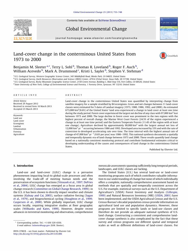
Fig. 1. (A) Six reporting regions partitioning the conterminous United States (MWCF is M

NAD is North American Deserts, GP is Great Plains, and ETF is Eastern Temperate Forests

time between 1973 and 2000 (% of ecoregion area).

Because of the extensive temporal record and relativelyconsistent spatial and radiometric characteristics, the Landsatseries of earth observation satellite data offer a unique opportunityto characterize changes between major land-cover classes across awide range of ecosystems. The Landsat archive, consisting of dataacquired by 6 satellites over a period of 40 years, offers a consistentsource of appropriate resolution observational data that is criticalto permit quantification of land change over sufficiently long timeperiods.

The objective of the U.S. Geological Survey Land Cover Trendsproject (Loveland et al., 2002) was to estimate the rates and typesof recent historical land-cover change across ecoregions of theconterminous U.S. (Loveland et al., 2002; Stehman et al., 2003a)(hereafter, we will omit the modifier ‘‘conterminous’’ but allreferences to the U.S. should be understood as meaning theconterminous U.S.). The major land-cover changes captured in thisstudy represent processes associated with forest harvest; urbani-zation; agricultural intensification, deintensification, and aban-donment; and mining. In this article we report broad-scalepatterns of land-cover change augmenting the national resultswith regional results presented for the following six regions:Eastern Temperate Forests, Great Plains, Western Cordillera,Marine West Coast Forests, North American Deserts, andMediterranean California (Fig. 1). National estimates of overallchange are first summarized by the land change footprint (orchange footprint) of the U.S., defined as the total area of land thatexperienced a change in land cover in at least one of the four timeintervals (1973–1980, 1980–1986, 1986–1992, and 1992–2000)partitioning the 1973–2000 study period. Regional estimates of

arine West Coast Forests, MC is Mediterranean California, WC is Western Cordillera,

), and (B) the estimated land change footprint, or the area that changed at least one

B.M. Sleeter et al. / Global Environmental Change 23 (2013) 733–748 735

overall change follow based on the land change footprint of the sixmajor regions. Results are then presented for three major types ofchange observed nationally: forest cover decline, urban expansion(increasing development), and agriculture loss. Complete resultscan be found in Dataset S1. Although the primary objective is toquantify land change, explanations of potential driving forcesaccompany some of the estimates of change. In depth regionalanalyses and studies focusing on causes and consequences ofchange based on the data collected in this study are in progress orin press, for example, land-cover change in California (Sleeter,2008; Sleeter et al., 2010) and the western U.S. (Sleeter et al.,2012a; Soulard and Sleeter, 2012), the Great Plains (Drummond,2007; Drummond et al., 2012) and the eastern U.S. (Drummondand Loveland, 2010; Napton et al., 2010; Auch et al., 2012; Sohl andSohl, 2012).

2. Materials and methods

A stratified random sample of 2688 10-km � 10-km blocks(some ecoregions used 20-km � 20-km blocks) was selected from84 ecoregion strata in the U.S. (Fig. 2) (Loveland et al., 2002;Stehman et al., 2003a). Ecoregions originally developed byOmernik (1987) and later modified by the U.S. EnvironmentalProtection Agency (1999) provided the spatial framework for thesampling design and analysis (Fig. 1, Table S1). Ecoregions havebeen demonstrated to be an effective framework for characterizingchanges in U.S. land cover (Gallant et al., 2004). Land cover wasclassified according to a modified version of the Anderson Level Iclassification scheme (Anderson et al., 1976) consisting of 11 landcover classes, water, developed, mining, barren, forest, grassland/shrubland, agriculture, wetland, snow/ice and two disturbanceclasses: mechanical (anthropogenic) and nonmechanical (natural)(Table 1). Landsat MSS, TM, and ETM+ images were used by

Fig. 2. Ecoregions, sample blocks, and 1992 land cover reclassified from the 1992 NLCD

schemes). Black lines are ecoregion boundaries and black boxes are the 2688 sample b

interpreters to identify and map changes in LULC betweensuccessive image dates. After classification, images were comparedto determine for each sample block the area of each possible type ofchange between the 11 land cover classes. The four changeintervals, 1973–1980, 1980–1986, 1986–1992, and 1992–2000,were selected to take advantage of time and cost savings gained byusing Landsat data that had already been radiometrically andgeometrically corrected. Annual rates of change were computed toallow comparisons between the different length time periods. It isimportant to note that while annualizing the period estimatesprovides a means of comparing the varying length temporalintervals, the annual rates ignore inter-period changes that mayhave been missed using our 6–8 year change intervals.

Methods used for this research are described in detail inLoveland et al. (2002) and Stehman et al. (2003a, b). Here weprovide a brief overview of the major methodological componentsof the research, including spatial and temporal sampling, theclassification system used to characterize land-cover change,techniques to classify land change, and finally the statisticalestimation of change.

2.1. Ecoregion stratification and sample selection

The regional stratification of the conterminous United States(U.S.) was based on the 1999 version of the EPA’s Level IIIecoregions of the U.S. (EPA, 1999) (Fig. 2). A fixed grid of 10-km � 10-km blocks (9 of the first ecoregions processed used 20-km � 20-km blocks) was overlaid on the ecoregion map and eachblock was assigned to an ecoregion based on the location of thecenter point of the block. Sliver (incomplete) blocks were foundalong coastlines and international borders. In these instances, thesliver blocks were attached to an adjacent ‘‘parent’’ block to ensurethat the area of the sliver blocks was eligible to be sampled. A

to the Table S1 classification (see Table S2 for ‘‘crosswalk’’ between classification

locks. Ecoregion numbers are shown in Table S2.

Table 1Land-cover classes and descriptions.

Class Description

Water Areas persistently covered with water, such as streams, canals, lakes, reservoirs, bays, or oceans.

Developed Areas of intensive use with much of the land covered with structures or anthropogenic impervious surfaces (e.g., high-density

residential, commercial, industrial, roads, etc.) or less intensive uses where the land cover matrix includes both vegetation and

structures (e.g., low-density residential, recreational facilities, cemeteries, parking lots, utility corridors, etc.), including any

land functionally related to urban or built-up environments (e.g., parks, golf courses, etc.).

Mining Areas with extractive mining activities that have a significant surface expression. This includes (to the extent that these features

can be detected) mining buildings, quarry pits, overburden, leach, evaporative, tailings, or other related components.

Barren Land comprised of soils, sand, or rocks where less than 10 percent of the area is vegetated. Barren lands are usually naturally

occurring.

Forest Tree-covered land where the tree-cover density is greater than 10 percent. Note that cleared forest land (i.e., clear-cuts) is

mapped according to current cover (e.g., mechanically disturbed or grassland/shrubland).

Grassland/shrubland Land predominately covered with grasses, forbs, or shrubs. The vegetated cover must comprise at least 10 percent of the area.

Agriculture Land in either a vegetated or an unvegetated state used for the production of food and fiber. This includes cultivated and

uncultivated croplands, hay lands, pasture, orchards, vineyards, and confined livestock operations. Note that forest plantations

are considered forests regardless of the use of the wood products.

Wetland Land where water saturation is the determining factor in soil characteristics, vegetation types, and animal communities.

Wetlands usually contain both water and vegetated cover.

Snow/ice Land where the accumulation of snow and ice does not completely melt during the summer period (e.g., alpine glaciers and

snowfields).

Mechanical disturbance Land in an altered and often unvegetated state that, due to disturbances by mechanical means, is in transition from one cover

type to another. Mechanical disturbances include forest clear-cutting, earthmoving, scraping, chaining, reservoir drawdown,

and other similar human-induced changes.

Nonmechanical disturbance Land in an altered and often unvegetated state that, due to disturbances by non-mechanical means, is in transition from one

cover type to another. Non-mechanical disturbances are caused by fire, wind, floods, animals, and other similar phenomena.


simple random sample was chosen from each ecoregion (stratum)with the sample size per ecoregion based on ecoregion size and theexpected variability of change within the ecoregion (Stehmanet al., 2003a, b). The first ecoregions sampled had the 20-km � 20-km sample blocks, but early results for these ecoregions indicatedthat more precise change estimates would be obtained if the blocksize was reduced. Sample sizes ranged from 9 to 11 blocks forecoregions using the 20-km blocks and 25 to 48 sample blocks forecoregions using the 10-km blocks. For some results reported inthis article, Level III ecoregions were aggregated into six macro-scale regions similar to Level I ecoregions (Table S1).

2.2. Temporal sampling and landsat data collections

Temporal sampling was designed to utilize as many low-cost orfree geometrically and radiometrically corrected datasets aspossible while preserving a 6–8 year interval between observa-tions. Equal length time periods would have been preferable, butthe time and cost savings associated with using existing satellitedata drove the decision to use time periods of different length (notethat this study was initiated prior to the 2008 decision to makeLandsat data available at no cost; future efforts to documentchange may afford more regular or frequent analyses). The fivedates were 1973, 1980, 1986, 1992, and 2000 with imagescollected �1 year from the center point dates. Landsat MultispectralScanner (MSS) triplicates from the North American LandscapeCharacterization (NALC) program (Lunetta and Sturdevant, 1993)were collected for 1973, 1986, and 1992. These data were precisionand terrain corrected and registered to a common map base to ensureaccurate pixel-to-pixel registration. For 1992 we also procuredLandsat Thematic Mapper (TM) data from the Multi-Resolution LandCharacteristics (MRLC) project which consists of precision and terraincorrected 30-m Landsat TM data used for production of the 1992National Land Cover Dataset (NLCD). For 2000, we used LandsatEnhanced Thematic Mapper Plus (ETM+) data from the MRLC 2001collection. This collection typically included three or more ETM+acquisitions collected between 1999 and 2002. In some cases TM datafrom Landsat 5 were also included. The only new data acquisitionrequired was for 1980. These data were ordered with Level 1systematic processing with terrain correction. All Landsat data were

processed to an Albers Conical Equal Area projection with MSS datareprojected to 60-m resolution and TM and ETM+ to 30-m resolution.

2.3. Classification scheme

Two primary factors affected the design of our classificationsystem. The first factor was recognizing that the use of moderate-resolution imagery Landsat TM/ETM+ and MSS would necessitate aland cover classification system that was fairly general in order toachieve high interpretation accuracy and consistency. Our abilityto identify and map land cover was limited by the technicalspecifications of the Landsat MSS, TM, and ETM+ sensors and by thelocal and regional landscape characteristics that affect the formand contrast visible in satellite imagery. This would be especiallytrue when interpreting Landsat MSS data. The second factorinvolved choosing classes that captured the land cover changes ofinterest. Since we were interested in land-use change with landcover serving as a surrogate for land use, we decided to use theAnderson Level I classes (Anderson et al., 1976) because thisclassification scheme was designed to provide land-use surrogates.To characterize lands that were in transition between cover types,we modified the Anderson system by adding two disturbancecategories; mechanically disturbed (human-induced) and non-mechanically disturbed (natural) (Table 1). The mechanicallydisturbed class was used to capture areas that had been recentlydisturbed by mechanical means and was particularly useful foridentifying areas that had experienced forest clear-cut logging.Mechanically disturbed lands also included other relatively minorchanges such as reservoir drawdown, scraping, earthmoving, andchaining, and other human-induced changes. The non-mechani-cally disturbed class was used to capture land altered bydisturbances, such as wildfire, and to a lesser extent, winds,floods, animals (e.g. beetle infestation), and other similarphenomena.

2.4. Mapping baseline land cover

We used the 1992 NLCD (Vogelmann et al., 2001) as a startingpoint for land-cover mapping. NLCD land cover was extracted foreach sample block and then reclassified to match our classification

Fig. 3. Example of Landsat TM (A), 1992 NLCD (B) and interpreted Trends land cover map (C). The example is from the Southern and Central California Chaparral and Oak

Woodlands Ecoregion. The legend shows the classification scheme used for this assessment and corresponding to the maps in panel B and C. The NLCD map in panel B was

reclassified to match the Land Cover Trends classification scheme (see Table S2 for ‘‘crosswalk’’ between classification schemes).


scheme (Table S2). Image interpreters then manually evaluatedthe reclassified NLCD by examining Landsat data and otherancillary sources such as aerial photography and topographicmaps and, using a minimum mapping unit of 60-m � 60-m,modified the NLCD product to produce a starting land-covermap for each sample block (Fig. 3). The overall accuracy of the1992 NLCD ranged from 70 to 83% in the four eastern federalregions of the U.S. Environmental Protection Agency (EPA)(Stehman et al., 2003a, b) and from 74 to 85% in the six westernEPA federal regions (Wickham et al., 2004), with considerablevariation in class-specific user’s and producer’s accuraciesamong regions. The reclassification, or interpreter ‘‘clean-up’’process, of the 1992 NLCD often resulted in substantialremapping of LULC to produce a reliable starting point forchange mapping.

2.5. Mapping land-cover change

Mapping land-cover change for each sample block requiredimage interpreters to visually inspect Landsat image pairs whilelooking for areas that experienced a change. Analysis was firstconducted between the 1992 and 2000 dates. The land cover mapmodified from the 1992 NLCD was used as a base for the 2000 yearwith areas of change identified and recoded in the 2000 land coverimage. Upon completion of the 2000 date, both the 1992 and 2000land cover images were resampled to 60-m resolution using thenearest neighbor technique. The new 60-m data from 1992 werethen used as a starting point for interpreting the 1986 land cover.Any change identified by comparing the 1992 and 1986 imagepairs was recoded into the 1986 land cover product. This processwas repeated until all five dates were complete. Upon completionof land-cover mapping, land-cover change images were producedusing simple thematic image differencing between each successiveimage pair. This resulted in 4 temporal periods of change imagesfor each sample block. Additionally, spatial land change ‘‘footprint’’

maps were produced showing the number of times each 60-mpixel within a sample block experienced a change (Fig. 4). Fig. 5shows an example of Landsat imagery, sample block interpreta-tion, and land-cover change images.

Validation of land cover mapping was achieved through anecoregion review process where all sample blocks wereexamined by the full team of image interpreters, includingthose who did not interpret sample blocks for the ecoregionbeing subjected to the quality assessment. This approachallowed for an independent critique of mapping while ensuringgeneral consistency with national-scale project methodologyand objectives. Areas of disagreement identified in the ecoregionreview process were reclassified to ensure as accurate aclassification as possible. The goal of the mapping effort wasto achieve as high of rates of accuracy as possible using Landsatdata as the primary interpretative source. Additionally, inter-preters regularly utilized other ancillary sources of data, such asaerial photographs and topographic maps, when conductingchange mapping to further increase the accuracy of Landsat-based interpretations.

2.6. Statistical estimation

Stratified random sampling formulas are used for estimatingarea and standard errors. The 84 Level III ecoregions are the stratafor the sampling design. Let yh,u denote an area for sample block u

of stratum h (e.g., yh,u is the area of forest in 1992 for sample block u

in one of the 84 ecoregion strata, or yh,u is the area of gross changeof forest to developed from 1986 to 1992 in block u of stratum h),and Nh and nh denote the number of blocks and number of blockssampled in stratum h (Table S1). For stratum h, the estimated totalarea is

bYh ¼ Nhyh

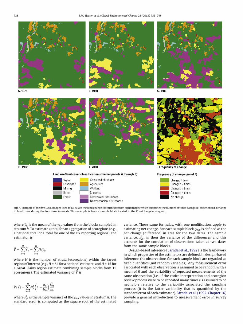
Fig. 4. Example of the five LULC images used to calculate the land change footprint (bottom right image) which quantifies the number of times each pixel experienced a change

in land cover during the four time intervals. This example is from a sample block located in the Coast Range ecoregion.


where yh is the mean of the yh,u values from the blocks sampled instratum h. To estimate a total for an aggregation of ecoregions (e.g.,a national total or a total for one of the six reporting regions), theestimator is

bY ¼XH

h¼1

bYh ¼XH

h¼1

Nhyh

where H is the number of strata (ecoregions) within the targetregion of interest (e.g., H = 84 for a national estimate, and H = 15 fora Great Plains region estimate combining sample blocks from 15ecoregions). The estimated variance of bY is

bVðbYÞ ¼XH

h¼1

N2h 1 � nh

Nh

� �s2

yh

nh

where s2yh is the sample variance of the yh,u values in stratum h. The

standard error is computed as the square root of the estimated

variance. These same formulas, with one modification, apply toestimating net change. For each sample block, yh,u is defined as thenet change (difference) in area for the two dates. The samplevariance, s2

yh, is then the variance of the differences and thisaccounts for the correlation of observations taken at two datesfrom the same sample blocks.

Design-based inference (Sarndal et al., 1992) is the frameworkin which properties of the estimators are defined. In design-basedinference, the observations for each sample block are regarded asfixed quantities (not random variables). Any measurement errorassociated with each observation is assumed to be random with amean of 0 and the variability of repeated measurements of thesame observation (i.e., if the entire interpretation and ecoregionreview process were to be repeated many times) is assumed to benegligible relative to the variability associated the samplingprocess (it is the latter variability that is quantified by thestandard error of each estimator). Sarndal et al. (1992, Chapter 16)provide a general introduction to measurement error in surveysampling.

Fig. 5. Land-cover interpretation and corresponding change images produced from manual interpretation of Landsat data. The top row in panel A contains Landsat MSS (first

three images), TM (fourth image) and ETM+ (last image) images. The second row in panel A depicts the interpreted land cover. Panel B displays the change and no change areas

for the four temporal intervals. The example is from the Texas Blackland Prairies ecoregion.


3. Results

This study focused on describing the geographic, temporal, andthematic dimensions of 1973–2000 U.S. land cover change. To aidin understanding these three dimensions, we will first describe thegeography of change – the land change footprint as it varies byecoregion and through time (Section 3.1), and then present thethematic transformations and how they vary over time (Section3.2). The thematic dimensions will focus on the three primarytransformations – forests and agricultural loss, and urbanexpansion. At the national scale, our results show LULC changeto be relatively rare, affecting 8.6% of the nation’s land area overour 27-year study period; however, change was highly variableacross ecological regions, ranging from as little as 0.5% to greaterthan 33%, with the highest rates occurring between 1986 and 1992.Cumulatively, LULC change resulted in the rapid expansion ofdeveloped lands and declines in forests and agriculture. Further-more, the area of disturbed lands increased significantly throughtime. Throughout the presentation of results we utilize 6 broadecological regions as a means of providing geographic context, andillustrate the large degree of spatial variability in our results.

3.1. The land change footprint

The land change footprint is the amount of land that changed atleast one time over the course of the full study period and wasestimated at 673,000 km2(8.6%) of the U.S. between 1973 and2000. Most of the changed area only experienced a change in asingle time period (63.1%), while 30.5% changed two times, and5.9% changed three times. Multiple changes were generallyattributable to cyclic land change processes, such as forest harvestand regrowth, while locations changing only once were moretypically associated with unidirectional processes such as urbani-zation.

The land change footprint was distributed heterogeneouslyacross space (Fig. 1B) and time (Fig. 6). The change footprint inindividual ecoregions over the 27-year period ranged from 0.5% to33.8% (percent of ecoregion area) with a median of 6.5% for the 84ecoregions. The rates and types of land-cover change variedtemporally as different change agents such as government policy,environmental regulation, global and national economic condi-tions, and regional weather and climate variability interacted indifferent ways to affect regional land-use demand (e.g., Brown

0.0%

0.5%

1.0%

1.5%

2.0%

2.5%

MWCF ETF MC WC GP NAD CONUSRegion

1973-1980

1980-1986

1986-1992

1992-2000Ar

ea c

hang

ed, p

erce

nt o

f reg

ion

per y

ear

Fig. 6. Estimated annual rate of land change (percent of region per year) by time interval and region (error bars represent standard error). The regions are Marine West Coast

Forests (MWCF), Eastern Temperate Forests (ETF), Mediterranean California (MC), Western Cordillera (WC), Great Plains (GP), North American Deserts (NAD) and the

conterminous United States (CONUS).


et al., 2005; Lubowski et al., 2008; Wright and Wimberly, 2013).The highest annual rate of change among the four time periodsoccurred between 1986 and 1992 with an estimated rate of47,000 km2 yr�1 (Dataset S1). This period was characterized by theconvergence of high rates of timber harvest (see Section 3.2.1),rapid urbanization (see Section 3.2.2), and initiation of a largefederal program designed to conserve marginal farmland (seeSection 3.2.3; Sullivan et al., 2004).

Of the six major regions of the U.S., the Marine West CoastForests had the highest land change footprint (on a percent areabasis) with an estimated 24.5% of the region experiencing a changein land cover between 1973 and 2000. This region, which coversless than 100,000 km2 in coastal California, Oregon and Washing-ton, has an extensive forestry legacy and two major metropolitanregions (Portland, Oregon and Seattle, Washington). Forestmanagement practices and expansion of developed areas (USDA,2001; Hobbs and Stoops, 2002; Auch et al., 2004) were the majorcontributors to overall change. The highest annual rate of change inthis region was 2.1% between 1986 and 1992. This trend waslargely driven by a steady increase in forest harvest activitythroughout the region in response to increased demands for highquality old growth timber (Daniels, 2005).

The second highest land change footprint occurred in theEastern Temperate Forests where an estimated 11.4% of the regionexperienced a change in land cover. Given its large size, more thanhalf of the change footprint in the U.S. was located in this region.Two of the ecoregions with the highest percent area of change werefound in the Eastern Temperate Forests; the Ouachita Mountainshad the highest change of any ecoregion at 33.8% and the South-Central Plains had a change footprint of 27.1%. The threeecoregions with the largest change in terms of area were all inthe Eastern Temperate Forests. These were the Southeastern Plains(68,508 km2), the South-Central Plains (42,179 km2), and theSouthern Coastal Plain (35,603 km2) ecoregions. The commontheme in each of these ecoregions was the presence of intensiveforestry activities, although reforestation of agricultural areas,urban-industrial expansion, and mining contributed to high ratesof change in some ecoregions (USDA, 2001; Drummond andLoveland, 2010). As with the Marine West Coast Forests, theEastern Temperate Forests experienced a peak annual rate of landchange between 1986 and 1992 at approximately 24,000 km2 yr�1.

The Mediterranean California region encompasses threehighly diverse ecoregions including the nation’s most populous

ecoregion, the Southern and Central California Chaparral and OakWoodlands (from here on called the ‘‘Oak Woodlands’’), whichincludes the San Diego, Los Angeles, and San Francisco-San Josemetropolitan areas. The land change footprint in MediterraneanCalifornia was estimated at 9.9%. With the exception of the 1986–1992 period (680 km2 yr�1), change was consistent over time atapproximately 850 km2 annually. However, the driving forces ofchange were spatially variable. Urbanization and wildfire wereimportant contributors of change in the Oak Woodlands, whileagricultural gross changes (gains and losses), driven in part bypressure for new urban lands and climate variability, wereimportant in the Central California Valley (Sleeter, 2008). Herethe annual rate of change was lower between 1986 and 1992(680 km2 yr�1) owing at least partially to a period of extended andprolonged drought.

In the Western Cordillera, the land change footprint wasestimated at 8.3% with the region accounting for approximately11% of the national estimated change. Land change in this regionwas primarily associated with forest disturbance includinglogging, wildfire, and more recently, insect-related forest die-off(Westerling et al., 2006). The annual rate of change increasedduring the first two time periods but then leveled off atapproximately 5700 km2 yr�1 for the 1986–1992 and 1992–2000 periods. The land change footprint in the Great Plains was8.1% and the region accounted for 25% of national LULC change. Theannual rate of change was twice as high between 1986 and 1992(12,600 km2 yr�1) as it was in previous time periods and waslargely the result of federal conservation policies in the 1985 U.S.Farm Bill that were designed to conserve highly erodible landsthrough conversion of agriculture to natural land covers (Drum-mond, 2007).

The region with the lowest land change footprint was the NorthAmerican Deserts at 2.7%. However, drivers of spatial variability inland change were highly localized, with agricultural changeaffecting ecoregions such as the Columbia Plateau and SnakeRiver Plain, urbanization playing an important role in the MojaveBasin and Range, and mining driving change in the Wyoming Basinand Central Basin and Range. The fluctuation in the spatial extentof water, wetlands, and barren was also important at a local scaleas changes were driven in response to land management practicesand regional climate and weather variability (Barnett and Pierce,2008; Auch et al., 2011; Soulard and Sleeter, 2012). As in otherregions, the 1986–1992 period had the highest rate of land-cover


change, although the driving forces varied across ecoregion. Forexample, CRP enrollments in the Columbia Plateau drove highrates of change regionally (Sullivan et al., 2004), while urbaniza-tion in the Mojave Basin and Range was the dominant driver ofhigh land-cover change during the same period.

3.2. Land cover transformations

Land cover transformations refer to the change in land coverfrom one type to another. We tracked transformations in landcover across 9 general land-cover classes and 2 disturbed classes.The majority of change across the U.S. involved the conversion to orfrom forest, agriculture, or development. While regionally impor-tant in some ecoregions, other changes such as those involvingwater, wetlands, barren land, mining, and snow/ice, account for asmall overall percentage of the national-scale land transforma-tions; changes in grassland/shrubland are discussed in the contextof development and agriculture transformations below. As such,from a national perspective this section focuses on the changesinvolving the three primary land-cover classes that were mostdynamic over the study period: forest, development, and agricul-ture.

3.2.1. Forest cover

Forest land is defined as tree-covered land where the tree-crown areal density is greater than 10 percent (Table 1). The forestclass therefore represents a biophysical state of forest coverirrespective of land use (e.g., an area that has been clear-cut oraffected by a stand replacing wildfire would not be classified asforest even though the potential ‘‘use’’ of the land may eventuallyresult in a return to forest cover).

3.2.1.1. Net forest change 1973–2000. Forests account for nearlyone third of the land surface area of the U.S. (Homer et al., 2007; Fryet al., 2011). An estimated 16.6% (367,000 km2) of the U.S. forestarea experienced a change in land cover at least once between1973 and 2000. Forest cover declined from an estimated2,305,500 km2 in 1973, to 2,208,300 km2 in 2000, a net loss of4.2% of 1973 forest area (Table 2). Our estimate is consistent withother forest assessment data for the U.S. For example, Hansen et al.(2010) used Landsat and MODIS (Moderate Resolution ImagingSpectroradiometer) to produce estimates of global gross forestcover loss and estimated 1,992,000 km2 of forest in the UnitedStates in the year 2000, an estimate similar to ours consideringtheir more conservative forest classification threshold of 25%canopy cover. The 2001 NLCD shows forests covered2,022,412 km2 based on a canopy cover requirement of 20% withminimum tree heights of 5 meters (Homer et al., 2007).

Forest-cover loss occurred throughout the United States as allsix major regions had less forest cover in 2000 than in 1973(Fig. 7). Combined, the Eastern Temperate Forests, WesternCordillera, and Marine West Coast Forests accounted for 94% ofthe net forest loss in the country. The Eastern Temperate Forestsaccounted for the most area change with a loss of 61,600 km2, adecline of 4.4% of the region’s forest cover and 63.3% of the totalnet forest loss estimated for the U.S. The Western Cordillera hadthe second highest amount of forest loss at 25,200 km2, a declineof 4.5% of regional forest cover and 25.6% of the nation’s netforest decline. The Marine West Coast Forests region had thehighest annual rate of forest loss (7.6%) in terms of percent ofarea and accounted for 4.7% of the national net loss of forest. Netforest cover decline was ubiquitous across ecoregions with 72of the 84 ecoregions analyzed experiencing a net decline inforest cover. Of the 42 ecoregions with greater than 30% forestcover, 39 experienced a net forest cover decline between 1973and 2000.

3.2.1.2. Gross forest change 1973–2000. Examining gross forestcover loss and gross forest cover gain provides additionalunderstanding of the forest-cover change dynamic. Nationallyfor 1973–2000, annual gross forest cover loss (11,300 km2 yr�1)outpaced gross forest cover gain (7700 km2 yr�1). Transition fromforest to mechanical disturbance (i.e. logging) accounted for thelargest area of gross forest-cover loss at 211,000 km2, nearly seventimes more area than any other type of forest loss transition.Change from forest to non-mechanical disturbance, developed, andagriculture each accounted for approximately 25,000 km2 of grossforest cover loss.

The Eastern Temperate Forests accounted for 78% of thenational area of gross loss of forest attributable to logging, 91% ofthe national gross loss attributable to agriculture, and 91% of thegross loss attributable to development. Gross forest cover gain inthe Eastern Temperate Forests resulted primarily from post-disturbance regrowth and reforestation of agricultural lands.Reforestation accounted for 25,000 km2 of gross forest gainbetween 1973 and 2000; however, these gains from reforestationwere largely offset by conversion of forest into new agriculturalareas as an estimated 23,000 km2 of forest land were broughtunder cultivation. The rate of forest to agriculture conversiondeclined over time from 1100 km2 yr�1for 1973–1980 to500 km2 yr�1for 1992–2000. The conversion of forests into newdeveloped areas accounted for an estimated 24,000 km2 and theannual rate of this conversion increased during the study period.During 1992–2000, approximately 1100 km2 yr�1 of forest werebeing converted in the Eastern Temperate Forests, up from700 km2 yr�1 between 1973 and 1980. Driving forces of forestchange were numerous. More forest was harvested in the South in1986 than any time since the 1920s (Walker, 1991). The legacy ofhigh interest rates of the late 1970s and the impacts of the early1980s recession, coupled with a substantial amount of salvagedtimber resulting from regional pine beetle outbreaks, causedincreased cutting to make up for falling stumpage prices (Walker,1991). The economic recovery by the second half of the 1980sallowed for more new construction; new housing starts in 1986were higher than any other year between 1978 and 2003 (NAHB,2012) and by 2000, southern ecoregions had become the nation’smost important commercial forest region.

Gross forest-cover loss in the Western Cordillera was drivenalmost entirely by disturbance with an estimated 15% of the lossattributable to mechanical disturbance and 76% attributable tononmechanical disturbance. The annual rate of mechanicaldisturbance accelerated, peaking at 1700 km2 yr�1between 1986and 1992, before declining to 900 km2 yr�1between 1992 and2000. Nonmechanical disturbances, primarily wildfire, accountedfor approximately 19,000 km2 of the gross forest cover loss in theWestern Cordillera. An estimated 100 km2 yr�1 of nonmechanicaldisturbance occurred in the Western Cordillera between 1973 and1986 was followed by an increase to 900 km2 yr�1 between 1986and 1992, and 1500 km2 yr�1 between 1992 and 2000. Increasedfuel loads (Pimentel et al., 2000), the introduction and/or spread ofinvasive species (Whisenant, 1990), and changes and variability inregional climate have been linked to increased natural disturbanceand forest die-off from insects and wildfire (Westerling et al.,2006).

Mechanical disturbance was the process most responsible forgross forest cover loss in the Marine West Coast Forests as anestimated 17% (15,000 km2) of the region experienced a conver-sion from forest to mechanically disturbed. As in the WesternCordillera, logging increased through each time period, reaching ahigh of 800 km2 yr�1 between 1986 and 1992 before declining to600 km2 yr�1 between 1992 and 2000. Declines in harvest in theregion, particularly in the Cascades ecoregion, were driven at leastpartially by declining demand from Asian markets (Daniels, 2005),

Table 2Estimated land-cover composition and 1973–2000 net change in class area for conterminous U.S. (national) and six reporting regions.

Area (km2)

National 1973 1980 1986 1992 2000 Net change

Water 194,237 197,217 200,839 199,581 207,430 13,193

Developed 235,461 252,350 266672 285369 312990 77529

Mechanical disturbance 38659 42368 55644 67688 73293 34634

Mining 13877 15874 16825 17235 17812 3935

Barren 65516 65390 64958 65323 65446 �69

Forest 2305566 2277778 2254588 2234558 2208293 �97273

Grassland/shrubland 2575125 2569731 2,568,919 2,622,304 2,623,884 48,759

Agriculture 2,125,437 2,137,088 2,132,841 2,060,969 2,035,930 �89,507

Wetland 300,767 297,246 293,466 294,407 287,127 �13,639

Nonmechanically disturbed 3550 3169 3463 10,785 26,055 22,505

Snow/ice 1939 1924 1917 1914 1873 �66

Marine West Coast Forests

Water 5560 5553 5573 5562 5541 �19

Developed 5001 5396 5806 6282 6975 1974


Mining 78 94 103 113 124 45

Barren 750 735 700 696 695 �55

Forest 59,380 58381 56808 54437 54842 �4538

Grassland/shrubland 2980 4098 4056 5030 4370 1390

Agriculture 12061 12056 11904 11647 11460 �600

Wetland 1133 1120 1121 1104 1109 �24

Nonmechanically disturbed 8 0 0 39 0 �8

Snow/ice 17 17 17 17 17 0

Eastern Temperate Forests

Water 146,836 149,300 151,508 152,872 154,361 7525

Developed 186,632 197,971 208,550 222,103 243,544 56,912

Mechanical disturbance 26,138 32,169 42,860 49,380 59,212 33,074

Mining 8561 9764 9870 9434 8946 385

Barren 3156 3155 2975 2914 2961 �195

Forest 1,402,393 1,380,900 1,362,148 1,353,678 1,340,799 �61,594

Grassland/shrubland 47,330 51,174 56,307 60,881 59,053 11,723

Agriculture 972,165 971,751 965,262 948,373 933,507 �38,658

Wetland 253,128 249,553 246,549 246,626 242,841 �10,287

Nonmechanically disturbed 162 760 471 238 1275 1113

Snow/ice 0 0 0 0 0 0

Mediterranean California

Water 2950 3105 3031 2925 3066 115

Developed 10,066 11,078 11,716 12,658 13,574 3509


Mining 290 288 287 276 329 39

Barren 432 431 432 432 440 8

Forest 26,789 26,014 26,497 26,468 25,293 �1496

Grassland/shrubland 79,959 78,273 77,861 78,370 75,299 �4660

Agriculture 43553 43644 43,638 42,725 43,035 �517

Wetland 1316 1393 1446 1465 1438 122


Snow/ice 0 0 0 0 0 0

Western Cordillera

Water 8916 9051 8868 9049 9017 101

Developed 3872 4295 4530 4965 5375 1503

Mechanical disturbance 8672 6384 7871 10,237 7183 �1489

Mining 1164 1247 1385 1458 1519 355

Barren 15,536 15,556 15,624 15,579 15,625 89

Forest 559,749 556,313 553,557 544,829 534,552 �25,198

Grassland/shrubland 292,439 297,864 298146 299735 306663 14224

Agriculture 28409 28599 29418 27768 26349 �2060

Wetland 7053 6934 6961 6912 6910 �143


Snow/ice 1789 1774 1768 1764 1724 �66

Great Plains

Water 24,813 24,529 25,721 24,596 30,187 5374

Developed 22,228 24,539 25,879 27,456 30,187 7959


Mining 1112 1358 1700 2012 2418 1305

Barren 11,402 11,274 11,016 11,501 11,451 49

Forest 108,076 107,112 106,658 106,205 105,599 �2478

Grassland/shrubland 929,715 920,141 916,967 963,589 967,988 38,273

Agriculture 978,506 987,824 989,370 940,726 931,783 �46,723

Wetland 28,310 28,709 28,153 28,731 25,255 �3055

Nonmechanically disturbed 1390 0 0 13 324 �1066

Snow/ice 0 0 0 0 0 0


Table 2 (Continued )

Area (km2)

National 1973 1980 1986 1992 2000 Net change

North American Deserts

Water 5162 5678 6138 4578 5259 97

Developed 7663 9071 10,191 11,905 13,334 5671


Mining 2671 3123 3480 3942 4476 1804

Barren 34,240 34,238 34,211 34,200 34,275 35

Forest 149,178 149,058 148,920 148,942 147,209 �1969

Grassland/shrubland 1,222,702 1,218,181 1,215,582 1,214,699 1,210,510 �12,192

Agriculture 90,743 93,215 93,249 89,730 89,796 �947

Wetland 9827 9536 9237 9570 9575 �252


Snow/ice 133 133 133 133 133 0

Fig. 7. (A) Map of level III ecoregions showing net change in forest cover between 1973 and 2000, expressed as a percent change in the class from 1973 (ecoregions with less

than 10 percent forest cover in 1973 are not shown), (B) composition of forest cover, expressed as a percent of region area, by region and time period (error bars represent

standard error of estimate), and (C) percent net change in forest cover, expressed as a percent of region area, by time interval (error bars represent standard error). The regions

are Marine West Coast Forests (MWCF), Eastern Temperate Forests (ETF), Mediterranean California (MC), Western Cordillera (WC), Great Plains (GP), North American Deserts

(NAD) and the conterminous United States (CONUS).


Fig. 8. Map of level III ecoregions showing net change in developed cover between 1973 and 2000, expressed as a percent change in the class area from 1973, (B) composition

of developed cover, expressed as a percent of region area, by region and time period (error bars represent standard error of estimate), and (C) percent net change in developed

cover, expressed as a percent of region area, by time interval (error bars represent standard error). The regions are Marine West Coast Forests (MWCF), Eastern Temperate

Forests (ETF), Mediterranean California (MC), Western Cordillera (WC), Great Plains (GP), North American Deserts (NAD) and the conterminous United States (CONUS).


passage of the Northwest Forest Plan in response to concerns overloss of habitat for endangered species (USDA, 1994), and increasedsoftwood imports from Canada (Daniels, 2005). Unlike the WesternCordillera, urbanization was an important driver of forest coverloss in two of the three ecoregions comprising the Marine WestCoast Forests. An estimated 1100 km2 of forests were converted todevelopment, with approximately 950 km2 located in the PugetLowland ecoregion.

3.2.2. Developed land cover

Development includes residential, industrial, commercial,transportation, and areas such as parks or other open spacessurrounded or otherwise dominated by an urban landscape(Anderson et al., 1976). In 1973, development accounted forapproximately 235,000 km2 and 3% of the U.S. land area. By 2000,development had increased by 33% to 313,000 km2 and accounted

for 4% of the U.S. land area (Fig. 8, Table 2). Increases in developedarea tracked closely with U.S. population growth, which increasedapproximately 38% between 1970 and 2000 (Hobbs and Stoops,2002).

The Eastern Temperate Forests accounted for the vast majorityof developed area in the U.S. (approximately 78%). The establish-ment of new developed areas accelerated over time, from1600 km2 yr�1between 1973 and 1980 to 2700 km2 yr�1 between1992 and 2000. In total, 244,000 km2, or 8% of the region, wasclassified as developed in the year 2000, including 24,000 km2

converted from forest and 25,000 km2 converted from agriculturesince 1973. Four ecoregions (Atlantic Coastal Pine Barrens,Northern Piedmont, Northeastern Coastal Zone, and the SouthernCoastal Plains) have greater than 20% of their area classified asdeveloped and all four are within the Eastern Temperate Forestsregion.

Fig. 9. (A) Map of level III ecoregions showing net change in agriculture cover between 1973 and 2000, expressed as a percent change in the class from 1973 (ecoregions with

less than 10 percent agriculture cover in 1973 are not shown), (B) composition of forest cover, expressed as a percent of region area, by region and time period (error bars

represent standard error of estimate), and (C) percent net change in agricultural cover, expressed as a percent of region area, by time interval (error bars represent standard

error). The regions are Marine West Coast Forests (MWCF), Eastern Temperate Forests (ETF), Mediterranean California (MC), Western Cordillera (WC), Great Plains (GP), North

American Deserts (NAD) and the conterminous United States (CONUS).


The Great Plains region accounted for nearly 10% of the U.S.developed land area in 2000. From 1973 to 2000, the area ofdeveloped land increased by 36% (Drummond et al., 2012). Anestimated 91% of new developed area came from agriculture(5000 km2) and grassland/shrubland (3000 km2). The pattern wassimilar in Mediterranean California. Development increased by35%, expanding from 6.1% of the region in 1973–8.2% in 2000, anincrease of 3500 km2. As in the Great Plains, the vast majority ofnew development originated from agriculture (2100 km2) andgrassland/shrubland (1100 km2).

The Marine West Coast Forests region experienced the secondhighest rate of growth in new developed areas. Development

expanded from 5.6% of the region in 1973–7.8% in 2000, a 40%increase. Forest cover was the primary source of new developmentwith 1200 km2 converting over the 27-year period; conversionfrom agriculture contributed an additional 500 km2. The largestpercentage change in developed area occurred in the NorthAmerican Deserts where there was a 74% increase in newdevelopment from an estimated 7700 km2 in 1973 to13,300 km2 in 2000. An estimated 68% of this new developmentoriginated from grassland/shrubland and 25% originated fromagriculture. Large and fast growing metropolitan cities, such as LasVegas, NV in the Mojave Basin and Range Ecoregion, Phoenix, AZ inthe Sonoran Basin and Range Ecoregion, and Salt Lake City, UT in


the Central Basin and Range Ecoregion were major contributors toincreased urbanization (Knowles-Yanez et al., 1999; Acevedo et al.,2006).

3.2.3. Agricultural land cover

Agricultural lands are characterized as any area used for theproduction of food and fiber, including cultivated cropland, pasture,orchards and vineyards, nurseries and ornamental horticultureareas, and confined livestock feeding operations. In 1973, agricultureaccounted for 2,125,000 km2 (27%) of the U.S. land area (Fig. 9). From1973 to 1980, agriculture expanded at a net rate of 1700 km2 yr�1,with nearly all of the net change occurring in the Great Plains region.Between 1980 and 1986, agriculture continued to expand in theGreat Plains at a rate of 300 km2 yr�1; however, net decline inagriculture in the Eastern Temperate Forests (1100 km2 yr�1)resulted in an overall loss nationally of approximately 4200 km2.Between 1986 and 1992 we estimate a total net decline of72,000 km2 of agricultural land. The highest annual rate of declinewas in the Great Plains at 8100 km2 yr�1, followed by the EasternTemperate Forests at 2800 km2 yr�1. Between 1992 and 2000, therate of loss slowed to 1100 km2 yr�1for the Great Plains and1900 km2 yr�1for the Eastern Temperate Forests. From 1973 to2000, agriculture had declined by approximately 90,000 km2

nationally, with 43% of the area of net loss occurring in the EasternTemperate Forests and 52% in the Great Plains (Fig. 9). Nationally,34,400 km2 of agriculture was converted to developed land. Gains inagriculture came primarily from grassland/shrubland (83,200 km2)and forest (25,300 km2).

Prior to 1973, U.S. agricultural production outpaced domesticdemand (Cochrane, 1993). A spike in grain exports during the1970s, coupled with inflation, increased the value of cropland andacreage in production (Cochrane, 1993; Hargreaves, 1993). By1985, a depressed agricultural economy and growing environ-mental concerns led to changes in federal farm policy. TheConservation Reserve Program (CRP) was first established in theFood Security Act of 1985 and was authorized to idle nearly160,000 km2 of cropland by 2002, mostly in grasslands in the GreatPlains, but also in forested areas in the South and elsewhere(Sullivan et al., 2004). Nationally, the gross loss of agriculture tograssland/shrubland was estimated to be 132,400 km2 and thegross loss to forest was 26,000 km2.

3.2.4. Discussion of results

LULC change is recognized as a major driver of globalenvironmental change with systemic and cumulative conse-quences (Turner et al., 1990). Systemic effects are the physicalimpacts of human activities such as changes to atmospheric CO2

and other greenhouse gasses, hydrology, and climate and weather.The accumulation of many smaller scale changes causes cumula-tive consequences including deforestation, biodiversity loss, anddegradation of other ecosystem services. Land use trends in the UShave various implications.

The stability of carbon stocks is a key concern. Land usechange between 1973 and 2000 affected the extent of forestcover, tilled soil, grassland, wetland, and other land covers thatcontribute to carbon and other biogeochemical fluctuation. The4.2% decline in forest cover has implications for loss of standingcarbon to urbanization and timber harvest, though some carbonremains as woody debris after harvest and accumulates insecondary growth. However, there is regional variation inbiomass, growth rate, and soil carbon storage between Northern,Eastern Temperate, and Western forests (Liu et al., 2007). Aswell, the causes and extent of forest changes are regionally andtemporally variable.

Carbon sequestration in soils is affected when grassland cover isreplaced with a cropping regime. The substantial increase of

grassland/shrubland in agricultural regions since 1986, driven inlarge part by the CRP, is important to carbon dynamics. Landsconverted to CRP are small but reliable carbon sinks (Gebhart et al.,1994). Over the long term, CRP lands have a much larger impactdue to prevention of further carbon loss and biodiversity and waterquality benefits (Gelfand et al., 2011).

Climate and land cover interact through biogeophysicalprocesses that effectively make cropland, forests and cities acomponent of climate and weather systems (Pielke et al., 2007).Land use also has important but under-studied consequences forhydrology, including shifting water demands and changes in watersupply caused by human-altered hydrologic processes (Defrieset al., 2004). Natural disturbance, forest clearing, and landconversion to agriculture and urbanization affect surface albedoand hydrology, which ultimately affect regional weather andclimate (Barnes and Roy, 2008; Lawrence and Chase, 2010). Ourresearch suggests that there is often a mix of expanding,contracting, and stable land use and land cover types acrossregions that need to be considered in a comprehensive manner inorder to better understand forcings and feedbacks.

Local changes in forest, urban, and agricultural land uses have acumulative effect on regional and national land cover extent,pattern, and composition that affect habitat, biota, and otherenvironmental and socioeconomic conditions. The loss of forestcover identified here is counter to assumptions that the US and theeastern forests in particular are still undergoing a forest transitionfrom historical deforestation to a period of expanding forest cover(Mather, 1992). The net decline in forest that occurred throughoutthe study period affects habitat and the types of species that occuracross a range of ecological systems. Large and unfragmented coreforested areas are required by some birds and other species(Robinson et al., 1995). Conversely, the increases in grassland/shrubland in the Great Plains since 1986 are beneficial to manywildlife species (McLachlan et al., 2007). The acceleration of urbangrowth and other land use changes have transformed a substantialfraction of the US and contributed to human well-being but also todetrimental changes to ecosystem services that may be exacer-bated by a changing climate (Millennium Ecosystem Assessment,2005).

4. Conclusion

Previous land cover monitoring efforts in the U.S. lacked thespatial, temporal, and thematic consistency required to character-ize the rates and types of land-cover change at a spatial andtemporal scale useful for environmental management (Lovelandand Merchant, 2004). Quantifying land change via a nationally andtemporally consistent methodology enabled the direct comparisonof estimates of gross and net changes in land cover across timeperiods and ecoregions of the conterminous U. S. The national storyof U.S. land-cover change during 1973–2000 is that change is apervasive and variable phenomenon. There is significant geo-graphic and temporal variability in land-cover change. Someregions (e.g., southeast and northwest) are undergoing almostcontinuous change while others are relatively stable (e.g.,southwest deserts). The resource potential, controlled by regionalenvironmental variables including climate, topography, and soilsdetermine the dominant land uses, the probable transformations,and intensity of land management. The most dynamic regions arethose in which environmental conditions such as climate, soils, andtopography are suitable for productive and relatively intensiveresource-based land uses.

An estimated 8.6% of the U.S. landscape (an area roughly the sizeof Texas) underwent at least one land-cover change between 1973and 2000. Forest change was a major contributor to the dynamiclandscape with forest management (harvest and regeneration)


responsible for a large area of change. As a result of cyclic harvestingand regeneration, at any given time, a significant amount of land is intransition from forest cover to disturbed bare ground to grasses andshrubs. These transitions, especially the bare soil disturbed phase,may have important but temporary environment impacts. Althougha large proportion of the estimated 97,000 km2 of net forest loss maybe land temporarily in a disturbed or transitional grassland/shrubland state, 25,000 km2 of forest was converted to developmentand agriculture.

The addition of an estimated 77,000 km2 of development (anarea slightly less than South Carolina) will surely have substantialconsequences on ecosystem services. The net loss of agriculturalland is another significant story of U.S. land-cover change. Notsurprisingly, a substantial amount of the agricultural area lost wasto developed, but agriculture conversion to grassland/shrublandwas also common.

Numerous different, and often complex, interactions betweensocioeconomic drivers and biophysical characteristics haveproduced widespread ecoregional and temporal variability inthe rates, total extent, and types of U.S. land change. Regionalchanges are the cumulative result of individual land owner andland manager decisions on how to optimize the generation ofdesired benefits. Decisions are shaped by a complex set of factorsincluding resource potential, economics, technology, governmentpolicy, and land use history.

Key regional trends and causes emerged, as well as singularevents and actions that led to punctuated episodes of change. Thecharacterization and quantification of regional trends in LULC overlarge areas provides an important foundation for a wide range ofenvironmental and ecological research activities, including model-ing the linkages and feedbacks between land change andbiogeochemical cycling (Liu et al., 2006), the exchange of energybetween the land and atmosphere (Barnes and Roy, 2008), and thedevelopment and downscaling of global scenarios (Sleeter et al.,2012a, b). The results presented here are an important contribu-tion to a long-term land change-monitoring program capable ofmeeting the needs of the global change research community.

This study was designed based on constraints (e.g., Landsat datacosts) that are no longer an issue. The 2008 decision to make allLandsat data available at no cost means that future studies canmake greater use of the temporal richness of the Landsat archive(Wulder et al., 2012). Recent research is showing that by using theLandsat time series, change can be mapped with greater accuracyusing automated methods and that by using the full Landsathistory for a given place, change may soon be detectable shortlyafter it occurs (Zhu et al., 2012). Based on this study, we havedemonstrated that change is an uncommon event (the annualaverage rate of change ranged from 0.3 to 0.6 percent over time) atthe national level, but very high change rates occur in someregions. Because change rates are so variable in time and space,change will be better understood when we evolve into thecontinuous, wall-to-wall mapping and monitoring of land change.However, wall-to-wall maps of change have limitations associatedwith the accuracy and precision of change statistics. In the future,sampling, combined with wall-to-wall mapping (see Hansen et al.,2008), can provide both the geospatial results needed for modelingand assessing the consequences of change and the definitivestatistics that allow us to clearly and accurately understand thecomplex geographic, temporal, and thematic dimensions ofchange.

Appendix A. Supplementary data

Supplementary data associated with this article can be found, in

the online version, at doi:10.1016/j.gloenvcha.2013.03.006.

References

Acevedo, W., Taylor, J.L., Hester, D.J., Mladinich, C.S., Glavac, S. (Eds.), 2006. Rates,trends, causes, and consequences of urban land-use change in the United States.U.S. Geological Survey Professional Paper 1726.

Achard, F., Eva, H.D., Stibig, H-J., Mayaux, P., Gallego, J., Richards, T., Malingreau, J-P.,2002. Determination of deforestation rates in the world’s humid tropicalforests. Science 297, 999–1002.

Anderson, J.R., Hardy, E.E., Roach, J.T., Witmer, R.E., 1976. A land use and land coverclassification system for use with remote sensor data. U.S. Geological SurveyProfessional Paper 964, U.S. Government Printing Office, Washington, D.C.

Auch, R.F., Taylor, J.L., Acevedo, W., 2004. Urban growth in American cities: glimpsesof urbanization, U.S. Geological Survey Circular 1252, U.S. Government PrintingOffice, Washington, DC.

Auch, R.F., Sayler, K.L., Napton, D.E., Taylor, J.L., Brooks, M.S., 2011. Ecoregionaldifferences in late-20th century land-use and land-cover change in the U.S.Northern Great Plains. Great Plains Research 21 (Fall) 231–243.

Auch, R.F., Napton, D.E., Kambly, S., Moreland Jr., T.R., Sayler, K.L., 2012. The drivingforces of land change in the Northern Piedmont of the United States. GeographyReview 102 (1) 53–75.

Barnes, C.A., Roy, D.P., 2008. Radiative forcing over the conterminous United Statesdue to contemporary land cover land use albedo change. Geophysical ResearchLetters 35 (L09706) 1–6.

Barnett, T.P., Pierce, D.W., 2008. When will Lake Mead go dry? Water ResourcesResearch 44 (W03201) 1–10.

Brown, D.G., Johnson, K.M., Loveland, T.R., Theobald, D.M., 2005. Rural land usetrends in the Conterminous U.S., 1950–2000. Ecological Applications 15,1851–1863.

Caspersen, J.P., Pacala, S.W., Jenkins, J.C., Hurtt, G.C., Moorcroft, P.R., Birdsey, R.A.,2000. Contributions of land-use history to carbon accumulation in U.S. forests.Science 290, 1148–1151.

Cochrane, W.W., 1993. The Development of American Agriculture A HistoricalAnalysis, 2nd ed. University of Minnesota Press, Minneapolis153–156.

Committee on Global Change Research, 1999. Global Environmental Change: Re-search Pathways for the Next Decade. National Academy Press, Washington, DC.

Daniels, J.M., 2005. The Rise and Fall of the Pacific Northwest Log Export Market,General Technical Report PNW-GTR-624. U.S. Department of Agriculture, ForestService, Pacific Northwest Research Station.

DeFries, R.S., Foley, J.A., Asner, G.P., 2004. Land-use choices: balancing human needsand ecosystem function. Frontiers in Ecology and the Environment 2, 249–257.

Dobson, J.E., Bright, E.A., Ferguson, R.L., Field, D.W., Wood, L.L., Haddad, K.D., Iredale,H., III, Jensen, J.R., Klemas, V.V., Orth, R.J., Thomas, J.P., 1995. NOAA CoastalChange Analysis Program (C-CAP): Guidance for Regional Implementation,NOAA Technical Report NMFS 123, National Oceanographic and AtmosphericAgency, Seattle, Washington.

Drummond, M.A., 2007. Regional dynamics of grassland change in the westernGreat Plains. Great Plains Research 17, 133–144.

Drummond, M.A., Loveland, T.R., 2010. Land-use pressure and a transition to forest-cover loss in the Eastern United States. Bioscience 60 (4) 286–298.

Drummond, M.A., Auch, R.F., Karstensen, K.A., Sayler, K.L., Taylor, J.L., Loveland, T.R.,2012. Land change variability and human–environment dynamics in the UnitedStates Great Plains. Land Use Policy 29, 710–723.

EPA (Environmental Protection Agency), 1999. Primary distinguishing character-istics of Level III ecoregions of the continental United States. EnvironmentalProtection Agency http://www.epa.gov/wed/pages/ecoregions/level_iii.htm(accessed 10.05.99).

Fry, J.A., Xian, G., Jin, S., Dewitz, J.A., Homer, C.G., Yang, L., Barnes, C.A., Herold, N.D.,Wickham, J.D., 2011. Completion of the 2006 National Land Cover Database forthe conterminous United States. Photogrammetric Engineering and RemoteSensing 77, 858–864.

Gallant, A.L., Loveland, T.R., Sohl, T.L., Napton, D.E., 2004. Using an ecoregionframework to analyze land-cover and land-use dynamics. Environmental Man-agement 34 (1) S89–S110.

Gebhart, D.L., Johnson, H.B., Mayeux, H.S., Polley, H.W., 1994. The CRP increases soilorganic carbon. Journal of Soil and Water Conservation 49, 488–492.

Gelfand, I., Zenone, T., Jasrotia, P., Chen, J., Hamilton, S.K., Robertson, G.P., 2011.Carbon debt of Conservation Reserve Program (CRP) grasslands converted tobioenergy production. Proceedings of the National Academy of Sciences of theUnited States of America 110 (10) 4134–4139.

Gillespie, A.J.R., 1999. Rationale for a national annual forest inventory program.Journal of Forestry 97 (12) 16–20.

Hansen, M., Stehman, S., Potapov, P., 2010. Quantification of global gross forestcover loss. Proceedings of the National Academy of Sciences of the United Statesof America 107, 8650–8655.

Hansen, M.C., Stehman, S.V., Potapov, P.V., Loveland, T.R., Townshend, J.R.,Defries, R.S., Pittman, K.W., Arunarwati, B., Stolle, F., Steininger, M.K., Carroll,M., DiMiceli, C., 2008. Humid tropical forest clearing from 2000 to 2005quantified by using multitemporal and multiresolution remotely sensed data.Proceedings of the National Academy of Sciences of the United States ofAmerica 105, 9439–9444.

Hargreaves, M.W.M., 1993. Dry Farming in the Northern Great Plains Years ofReadjustment, 1920–1990. University Press of Kansas, Lawrence, KS.

Hobbs, F., Stoops, N., 2002. Demographic trends in the 20th century, U.S. CensusBureau, Census 2000 Special Reports, Series CENSR-4. U.S. Government PrintingOffice, Washington, DC.


http://refhub.elsevier.com/S0959-3780(13)00053-8/sbref0010






























http://www.epa.gov/wed/pages/ecoregions/level_iii.htm
























Homer, C., Dewitz, J., Fry, J., Coan, M., Hossain, N., Larson, C., Herold, N., McKerrow,A., VanDriel, J.N., Wickham, J., 2007. Completion of the 2001 National LandCover Database for the conterminous United States. Photogrammetric Engi-neering and Remote Sensing 73, 337–341.

Houghton, R., Hackler, J., Lawrence, K., 1999. The U.S. carbon budget: contributionsfrom land-use change. Science 285, 574–578.

Kalnay, E., Cai, M., 2003. Impact of urbanization and land-use change on climate.Nature 423, 528–531.

Knowles-Yanez, K., Moritz, C., Fry, J., Redman, C.L., Bucchin, M., McCartney, P.H.,1999. Historic Land Use: phase 1 report on generalized land use. CentralArizona-Phoenix long-term ecological research (CAPLTER), Arizona State Uni-versity, Tempe, AZ, 21 pp.

Lawrence, P.J., Chase, T.N., 2010. Investigating the climate impacts of global landcover change in the community climate system model. International Journal ofClimatology 30, 2066–2087.

Liu, J., Liu, S., Loveland, T.R., 2006. Temporal evolution of carbon budgets of theAppalachian forests in the U.S. from 1972 to 2000. Forest Ecology and Manage-ment 222, 191–201.

Loveland, T.R., Merchant, J.W., Ohlen, D.O., Brown, J.F., 1991. Development of a landcover characteristics database for the Conterminous U.S. PhotogrammetricEngineering and Remote Sensing 57 (11) 1453–1463.

Loveland, T.R., Sohl, T.L., Stehman, S.V., Gallant, A.L., Sayler, K.L., Napton, D.E., 2002.A strategy for estimating the rates of recent United States land-cover changes.Photogrammetric Engineering and Remote Sensing 68, 1091–1099.

Loveland, T.R., Merchant, J.M., 2004. Ecoregions and ecoregionalization: geographi-cal and ecological perspectives. Environmental Management 34, S1–S13.

Lubowski, R.N., Plantinga, A.J., Stavins, R.N., 2008. What drives land-use change inthe United States? A national analysis of landowner decisions. Land Economics84, 529–550.

Lunetta, R.S., Sturdevant, J.A., 1993. The North American Landscape Characteriza-tion Landsat Pathfinder Project. In: Pettinger, L.R. (Ed.), Pecora 12 Symposium,Land Information from Space-Based Systems, Proceedings, Bethesda, MD,American Society of Photogrammetry and Remote Sensing, pp. 363–371.

Mather, A.S., 1992. The forest transition. Area 24, 367–379.McLachlan, M., Carter, M., Rustay, C., 2007. Effects of the Conservation Reserve

Program on Priority Mixed-grass Prairie Birds. USDA Natural Resources Con-servation Service, WA.

Millennium Ecosystem Assessment, 2005. Ecosystems and Human Well-being:Biodiversity Synthesis. World Resources Institute, Washington, DC.

NAHB (National Association of Home Builders), 2012. Annual Housing Starts (1978–2011). http://www.nahb.org/generic.aspx?genericContentID=554 (accessed 4May).

Napton, D.E., Auch, R.F., Headley, R., Taylor, J.L., 2010. Land changes and their drivingforces in the Southeastern United States. Regional Environmental Change 10,37–53.

Omernik, J.M., 1987. Ecoregions of the conterminous United States. Annals of theAssociation of American Geographers 77, 118–125.

Pielke, R.A., Adegoke, J.O., Chase, T.N., Marshall, C.H., Matsui, T., Niyogi, D., 2007. Anew paradigm for assessing the role of agriculture in the climate system and inclimate change. Agriculture and Forest Meteorology 142, 234–254.

Pimentel, D., Lack, L., Zuniga, R., Morrison, D., 2000. Environmental and economiccosts of nonindigenous species in the United States. BioScience 50, 53–65.

Robinson, S.K., Thompson, F.R. III, Donovan, T.M., Whitehead, D.R., Faaborg, J., 1995.Regional forest fragmentation and the nesting success of migratory birds.Science 267 (5206) 1987–1990.

Sagan, C., Toon, O., Pollack, J., 1979. Anthropogenic albedo changes and the Earth’sclimate. Science 206, 1363–1368.

Sarndal, C.E., Swensson, B., Wretman, J., 1992. Model-assisted Survey Sampling.Springer-Verlag, New York.

Skole, D., Tucker, C., 1993. Evidence for tropical deforestation, fragmented habitat,and adversely affected habitat in the Brazilian Amazon: 1978–1988. Science260, 1905–1910.

Sleeter, B.M., 2008. Late 20th century land change in the Central California Valleyecoregion. The California Geographer 48, 27–59.

Sleeter, B.M., Wilson, T.S., Soulard, C.E., Liu, J., 2010. Estimation of late twentiethcentury land-cover change in California. Environmental Monitoring and As-sessment 173, 251–266.

Sleeter, B.M., Wilson T.S., Acevedo W, (Eds.), 2012. Status and Trends of Land Coverin the Western United States. U. S. Geological Survey Professional Paper 1794-A.

Sleeter, B.M., Sohl, T.L., Bouchard, M.A., Reker, R.R., Soulard, C.E., Acevedo, W.,Griffith, G.E., Sleeter, R.R., Auch, R.F., Sayler, K.L., Prisley, S., Zhu, Z., 2012b.Scenarios of land use and land cover change in the conterminous United States:utilizing the special report on emission scenarios at ecoregional scales. GlobalEnvironmental Change 22 (4) 896–914.

Sohl, T.L., Sohl, L.B., 2012. Land-use change in the Atlantic Coastal Pine BarrensEcoregion. Geography Review 102 (2) 180–201.

Soulard, C.E., Sleeter, B.M., 2012. Late twentieth century land-cover change in thebasin and range ecoregions of the United States. Regional EnvironmentalChange 12, 813–823.

Stehman, S.V., Sohl, T.L., Loveland, T.R., 2003a. Statistical sampling to characterizerecent United States land-cover change. Remote Sensing of Environment 86,517–529.

Stehman, S.V., Wickham, J.D., Smith, J.H., Yang, L., 2003b. Thematic accuracy of the1992 National Land-Cover Data (NLCD) for the Eastern United States: statisticalmethodology and regional results. Remote Sensing of Environment 86, 500–516.

Sullivan, P., Hellerstein, D., Hansen, L., Jihansson, R., Koenig, S., Lubowski, R.N.,McBride, W., McGranahan, D., Vogel, S., Roberts, M., Bucholtz, S., 2004. TheConservation Reserve Program economic implications for rural America. U.S.Department of Agriculture, Economic Research Service, Agricultural EconomicReport No. 834.

Turner, B.L.I.I., Kasperson, R.E., Meyer, W.B., Dow, K.M., Golding, D., Kasperson, J.X.,Mitchell, R.C., Ratick, S.J., 1990. Two types of global environmental change:definitional and spatial scale issues in their human dimensions. Global EnvironChange 1, 14–22.

USDA (U.S. Department of Agriculture), Forest Service; U.S. Department of theInterior, Bureau of Land Management, 1994. Final supplemental environmentalimpact statement on management of habitat for late-successional and old-growth forest related species within the range of the northern spotted owl.Portland, OR.

USDA (U.S. Department of Agriculture) Natural Resources Conservation Service,2001. Summary report: 1997 National Resources Inventory. U.S. Department ofAgriculture, Washington, D.C., 90 p. (revised December 2001).

Vitousek, P., Mooney, H., Lubchenco, J., Melillo, J., 1997. Human domination ofEarth’s ecosystems. Science 277, 494–499.

Vogelmann, J.E., Howard, S.M., Yang, L., Larson, C.R., Wylie, B.K., VanDriel, J.N., 2001.Completion of the 1990’s National Land Cover Dataset for the conterminousUnited States. Photogrammetric Engineering and Remote Sensing 67, 650–662.

Walker, L., 1991. The Southern Forest: A Chronicle. University of Texas Press,Austin, TX.

Westerling, A., Hidalgo, H., Cayan, D., Swetnam, T., 2006. Warming and earlierspring increase Western U.S. forest wildfire activity. Science 313, 940–943.

Whisenant, S., 1990. Changing Fire Frequencies on Idaho’s Snake River Plain:Ecological and Management Implications. U.S. Department of Agriculture ForestService, Intermountain Research Station, Ogden, UT.

Wickham, J.D., Stehman, S.V., Smith, J.H., Yang, L., 2004. Thematic accuracy of the1992 National Land-cover Data for the western United States. Remote Sensingof Environment 91, 452–468.

Wilbanks, T.J., Kates, R.W., 1999. Global change in local places: how scale matters.Climatic Change 43, 601–628.

Wright, C.K., Wimberly, M.C., 2013. Recent land use change in the western corn beltthreatens grasslands and wetlands. Proceedings of the National Academy ofSciences of the United States of America 110, 4134–4139.

Wulder, M.A., Masek, J.G., Cohen, W.B., Loveland, T.R., Woodcock, C.E., 2012.Opening the archive – how free data has enabled the science and monitoringpromise of Landsat. Remote Sensing of Environment 122, 2–10.

Zhu, Z., Woodcock, C.E., Olofsson, P., 2012. Continuous monitoring of forest distur-bance using all available Landsat imagery. Remote Sensing of Environment 122,75–91.



































http://www.nahb.org/generic.aspx?genericContentID=554


































































land-cover change in the conterminous united states from 1973 to 2000

Documents