land contamination correction for passive...

Land Contamination Correction for Passive Microwave Radiometer Data:Demonstration of Wind Retrieval in the Great Lakes Using SSM/I

JOHN XUN YANG

Department of Atmospheric, Oceanic and Space Sciences, University of Michigan, Ann Arbor, Michigan

DARREN S. MCKAGUE AND CHRISTOPHER S. RUF

Space Physics Research Laboratory, Department of Atmospheric, Oceanic and Space Sciences, University of

Michigan, Ann Arbor, Michigan

(Manuscript received 4 December 2013, in final form 29 July 2014)

ABSTRACT

Passivemicrowave radiometer data over the ocean have beenwidely used, but data near coastlines or over lakes

often cannot be used because of the large footprint with mixed signals from both land and water. For example,

current standard Special Sensor Microwave Imager (SSM/I) products, including wind, water vapor, and pre-

cipitation, are typically unavailable within about 100km of any coastline. This paper presents methods of cor-

recting land-contaminated radiometer data in order to extract the coastal information. The land contamination

signals are estimated, and then removed, using a representative antenna pattern convolved with a high-resolution

land–water mask. This method is demonstrated using SSM/I data over the Great Lakes and validated with sim-

ulated data and buoymeasurements. The land contamination is significantly reduced, and thewind speed retrieval

is improved. This method is not restricted to SSM/I and wind retrievals alone; it can be applied more generally to

microwave radiometer measurements in coastal regions for other retrieval purposes.

1. Introduction

Satellite-borne passive microwave radiometers have

been widely used in meteorology and climate studies

(Ulaby and Long 2014). In the open-ocean, retrieval

products, such as winds, water vapor, precipitation, wet

path delay, and sea ice, have been developed. However,

in coastal ocean areas or inland lakes and rivers, products

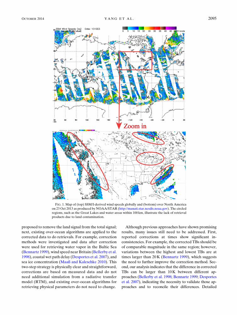
are often omitted. For example, Fig. 1 shows Special

Sensor Microwave Imager (SSM/I)-derived wind speeds

from standard products of the National Oceanic and

Atmospheric Administration’s (NOAA) Center for Sat-

ellite Application and Research (STAR; http://manati.

star.nesdis.noaa.gov), where coastal regions, including

the Great Lakes, show no retrievals. These limitations

also exist in the SSM/I water vapor and rain-rate prod-

ucts. The lack of retrieval products is due to the relatively

large footprint of SSM/I radiometers that covers both

land and water within a coastal field of view (FOV). The

additional land signals make retrievals over water using

standard open-ocean algorithms invalid. This phenome-

non is often referred to as land contamination. To further

illustrate the land contamination problem, Fig. 2 shows

an example of the observed brightness temperature (TB)

by SSM/I over the Great Lakes. Coastal areas of all lakes

are contaminated: in particular, the SSM/I footprint ex-

tends across all of Lake Ontario, so that all of the lake

data are contaminated. Because of land contamination,

coastal data have to be discarded without applying any

retrieval. However, coastal data contain important in-

formation on various physical parameters. For example,

the series of SSM/I instruments have documented more

than two decades of historical data that could provide

useful climatology information for coastal regions.

In the past, approaches for correcting land contami-

nation have been reported by other researchers. The

main strategy involves two steps toward extrapolating

coastal information: first, various techniques have been

Denotes Open Access content.

Corresponding author address: John Xun Yang, Department of

Atmospheric, Oceanic and Space Sciences,University ofMichigan,

2455 Hayward Street, Ann Arbor, MI 48109-2143.

E-mail: [email protected]

2094 JOURNAL OF ATMOSPHER IC AND OCEAN IC TECHNOLOGY VOLUME 31

DOI: 10.1175/JTECH-D-13-00254.1

� 2014 American Meteorological Society

http://manati.star.nesdis.noaa.gov


mailto:[email protected]

proposed to remove the land signal from the total signal;

next, existing over-ocean algorithms are applied to the

corrected data to do retrievals. For example, correction

methods were investigated and data after correction

were used for retrieving water vapor in the Baltic Sea

(Bennartz 1999), wind speed near Britain (Bellerby et al.

1998), coastal wet path delay (Desportes et al. 2007), and

sea ice concentration (Maaß and Kaleschke 2010). Thistwo-step strategy is physically clear and straightforward,

corrections are based on measured data and do not

need additional simulation from a radiative transfer

model (RTM), and existing over-ocean algorithms for

retrieving physical parameters do not need to change.

Although previous approaches have shown promising

results, many issues still need to be addressed. First,

reported corrections at times show significant in-

consistencies. For example, the corrected TBs should be

of comparable magnitude in the same region; however,

variations between the highest and lowest TBs are at

times larger than 20K (Bennartz 1999), which suggests

the need to further improve the correction method. Sec-

ond, our analysis indicates that the difference in corrected

TBs can be larger than 10K between different ap-

proaches (Bellerby et al. 1998; Bennartz 1999; Desportes

et al. 2007), indicating the necessity to validate those ap-

proaches and to reconcile their differences. Detailed

FIG. 1. Map of (top) SSM/I-derived wind speeds globally and (bottom) over North America

on 23 Oct 2013 as produced by NOAA/STAR (http://manati.star.nesdis.noaa.gov). The circled

regions, such as the Great Lakes and water areas within 100 km, illustrate the lack of retrieval

products due to land contamination.

OCTOBER 2014 YANG ET AL . 2095


comparison results are shown below. Third, error sources

affecting correction have not been completely con-

sidered. For example, spacecraft navigation errors di-

rectly affect the estimation of land signals; however,

such errors were ignored or assumed to be static pre-

viously, and this would produce significant errors in the

corrected data. Furthermore, the antenna pattern was

typically approximated using aGaussian pattern (Bennartz

1999; Desportes et al. 2007; Drusch et al. 1999; Maaß andKaleschke 2010). Our analysis found that this is a poor

approximation that does not have sidelobes. In coastal

regions, using an inappropriate antenna pattern can re-

sult in larger errors than in the open ocean, since TBs are

quite different between land and water. Last, the quality

of corrected data was not well validated—both removing

land-contaminated TBs and retrieval algorithm tuning

were often implemented to improve the quality of prod-

ucts near land.When only showing the retrieval products,

it is unclear from which the improvements come. In

general, there should be two validations. The first is for

the corrected TB, which can be compared with simu-

lated TBs over water using the RTM. This validation is

important because the quality of corrected TBs is the

most important aspect of the correction method; how-

ever, it was not presented in previous studies (Bellerby

et al. 1998; Bennartz 1999; Desportes et al. 2007; Maaßand Kaleschke 2010). A second validation should con-

firm the retrieved physical parameters from the cor-

rected data with independent observations (Bennartz

1999; Desportes et al. 2007; Maaß and Kaleschke 2010).It is insufficient to solely implement the second valida-

tion, because retrieval algorithms are often tuned to

match observations to compensate for TB errors.

In this study, we examine methods for correcting land

contamination. Different techniques are studied and the

optimal method is proposed. The corrected TBs are

analyzed and validated with simulated TBs. The appli-

cation of the corrected data is demonstrated using

a wind retrieval algorithm and validated with surface

buoy measurements. It is shown that the method pro-

duces well-corrected coastal retrievals. The retrieved

wind speed is validated with reference buoy measure-

ments. These results indicate that the proposed land

contamination correction method can be used to obtain

coastal information that would otherwise be absent and

thus fill a gap in current standard retrieval products.

2. Methodology and algorithms

A flowchart describing the overall approach of the

land contamination correction algorithm is shown in

Fig. 3. The algorithm consists of three parts: geolocation

corrections, land fraction estimationwith an appropriate

antenna patterns, and contamination removal. A dataset

with accurate geolocation is necessary, from which the

fraction of land contamination is calculated using a high-

resolution land–water mask convolved with a realistic

antenna pattern. The land signal can then be removed

using the correlation of multiple measurements around

the FOV.

a. Geolocation correction

Geolocation correction relates to the spacecraft

ephemeris (its 3D position of latitude, longitude, and

altitude as a function of time), attitude (roll, pitch, and

yaw position), and the projection of the radiometer an-

tenna pattern onto the Earth’s surface. Without proper

geolocation, the position of the FOV and Earth incident

angle (EIA) will have large errors, which affects any

subsequent analysis. For example, geolocation error can

propagate into calculated land fractions and result in

FIG. 2. An example of (top) land contamination over the Great

Lakes and (bottom) the corresponding SSM/I scan geometry. In

(top), overwater TBs close to coastlines (shaded yellow) are higher

than that at the center of the lakes (shaded blue) due to land

contamination. For example, all of Lake Ontario is contaminated,

since the SSM/I footprint is larger than the entirety of Lake On-

tario. (bottom) The solid line is the spacecraft ground track, the

dotted line is for the center of each SSM/I sample in a single azi-

muthal scan, and the green ellipse is a single antenna footprint.


overestimating or underestimating land signals. Although

preliminary geolocation examination is often provided

with standard radiometer data products, it is often not

accurate enough, andmore thorough processing is needed

(Berg et al. 2013; Poe and Conway 1990). In coastal re-

gions, accurate geolocation is more important than over

the open ocean because land and water TBs are quite

different, such that small errors from geolocation will lead

to large errors in the TB correction. Although this prob-

lem was suggested as an important error source in the

past, no specific solutions have been applied (Bellerby

et al. 1998; Bennartz 1999; Desportes et al. 2007; Maaßand Kaleschke 2010).Geolocation correction can be implemented by exam-

ining the coastline shift, since land and water have

significant TB contrast. Ground coordinates of data can

be aligned bymatching the coastline between the TBmap

and an accurate map of the land–water mask. Further-

more, parameters of spacecraft attitude can be retrieved

and used to calculate the correct ground coordinates. For

SSM/I, this coastline-based approach reduces geolocation

uncertainties from 20–30 to 10–12km relative to onboard

telemetry/ephemeris (Poe and Conway 1990). More re-

cent methods further improve geolocation accuracy to

uncertainties of less than 5km and reduced EIA un-

certainty from 0.58 to 0.18 (Berg et al. 2013). A brief in-

troduction is given about the technique (Berg et al. 2013).

The 85h channel was used to examine coastline shift. It has

the smallest footprint among SSM/I channels and has

larger land–water contrast than 85v, since emissivity dif-

ference between land andwater is larger for the horizontal

polarization channel (H-pol) than the vertical polarization

channel (V-pol). Ascending and descending orbits are

separated to examine coastline shift. The coasts of Aus-

tralia and Japan can be used to checkwest–east and north–

south directions. In addition, 19v and 37v are used to

examine spacecraft attitude and distinguish roll and yaw,

becauseV-pol ismore sensitive toEIA change thanH-pol.

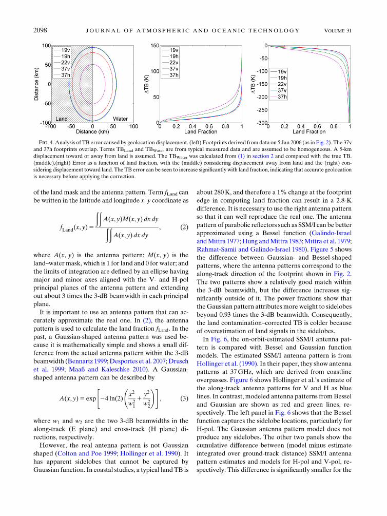
An illustration of the impact of geolocation error is

shown in Fig. 4. A geolocation displacement of 5 km is

assumed, and the corresponding error impacting the

correction is shown as a function of the land fraction.

Quantitative details for calculating the error can be

found in the following section. Qualitatively, the error

comes from either overestimation or underestimation of

the land fraction, depending on whether the displace-

ment is toward or away from the land. In either case, the

error increases with the land fraction. For example

the TB error exceeds 20K at a land fraction of 0.5 for

a 5-km displacement. The analysis indicates that a data-

set of very high-quality geolocation is important. In this

study, we used the latest dataset from Colorado State

University with its geolocation corrections applied (Berg

et al. 2013). It should be noted that Fig. 4 is for single

footprint analysis, whereas using multiple pixels is dif-

ferent because it can tolerate larger error. We will com-

pare the two different methods later.

b. Land contamination correction: Calculating landfraction using proper antenna pattern

Land contamination correction refers to the process

of removing the land signal from the measured TB. The

measured TB can be written as

TB5 fLandTBLand 1 (12 fLand)TBWater , (1)

where TBLand and TBWater are the TBs of land and water,

respectively. Term fLand is computed as the convolution

FIG. 3. Flowchart of the land contamination correction algo-

rithm. The correction consists of three parts: geolocation correc-

tion, land fraction estimation using appropriate antenna patterns,

and land contamination removal.


of the landmask and the antenna pattern. Term fLand can

be written in the latitude and longitude x–y coordinate as

fLand(x, y)5

ððA(x, y)M(x, y) dx dyðð

A(x, y) dx dy

, (2)

where A(x, y) is the antenna pattern; M(x, y) is the

land–water mask, which is 1 for land and 0 for water; and

the limits of integration are defined by an ellipse having

major and minor axes aligned with the V- and H-pol

principal planes of the antenna pattern and extending

out about 3 times the 3-dB beamwidth in each principal

plane.

It is important to use an antenna pattern that can ac-

curately approximate the real one. In (2), the antenna

pattern is used to calculate the land fraction fLand. In the

past, a Gaussian-shaped antenna pattern was used be-

cause it is mathematically simple and shows a small dif-

ference from the actual antenna pattern within the 3-dB

beamwidth (Bennartz 1999; Desportes et al. 2007; Drusch

et al. 1999; Maaß and Kaleschke 2010). A Gaussian-

shaped antenna pattern can be described by

A(x, y)5 exp

"24 ln(2)

x2

w21

1y2

w22

!#, (3)

where w1 and w2 are the two 3-dB beamwidths in the

along-track (E plane) and cross-track (H plane) di-

rections, respectively.

However, the real antenna pattern is not Gaussian

shaped (Colton and Poe 1999; Hollinger et al. 1990). It

has apparent sidelobes that cannot be captured by

Gaussian function. In coastal studies, a typical land TB is

about 280K, and therefore a 1% change at the footprint

edge in computing land fraction can result in a 2.8-K

difference. It is necessary to use the right antenna pattern

so that it can well reproduce the real one. The antenna

pattern of parabolic reflectors such as SSM/I can be better

approximated using a Bessel function (Galindo-Israel

andMittra 1977; Hung andMittra 1983;Mittra et al. 1979;

Rahmat-Samii and Galindo-Israel 1980). Figure 5 shows

the difference between Gaussian- and Bessel-shaped

patterns, where the antenna patterns correspond to the

along-track direction of the footprint shown in Fig. 2.

The two patterns show a relatively good match within

the 3-dB beamwidth, but the difference increases sig-

nificantly outside of it. The power fractions show that

theGaussian pattern attributesmore weight to sidelobes

beyond 0.93 times the 3-dB beamwidth. Consequently,

the land contamination–corrected TB is colder because

of overestimation of land signals in the sidelobes.

In Fig. 6, the on-orbit-estimated SSM/I antenna pat-

tern is compared with Bessel and Gaussian function

models. The estimated SSM/I antenna pattern is from

Hollinger et al. (1990). In their paper, they show antenna

patterns at 37GHz, which are derived from coastline

overpasses. Figure 6 shows Hollinger et al.’s estimate of

the along-track antenna patterns for V and H as blue

lines. In contrast, modeled antenna patterns fromBessel

and Gaussian are shown as red and green lines, re-

spectively. The left panel in Fig. 6 shows that the Bessel

function captures the sidelobe locations, particularly for

H-pol. The Gaussian antenna pattern model does not

produce any sidelobes. The other two panels show the

cumulative difference between (model minus estimate

integrated over ground-track distance) SSM/I antenna

pattern estimates and models for H-pol and V-pol, re-

spectively. This difference is significantly smaller for the

FIG. 4. Analysis of TB error caused by geolocation displacement. (left) Footprints derived from data on 5 Jan 2006 (as in Fig. 2). The 37v

and 37h footprints overlap. Terms TBLand and TBWater are from typical measured data and are assumed to be homogeneous. A 5-km

displacement toward or away from land is assumed. The TBWater was calculated from (1) in section 2 and compared with the true TB.

(middle),(right) Error as a function of land fraction, with the (middle) considering displacement away from land and the (right) con-

sidering displacement toward land. The TB error can be seen to increase significantly with land fraction, indicating that accurate geolocation

is necessary before applying the correction.


Bessel function than for the Gaussian. A few minor

points are 1) Hollinger et al.’s antenna pattern estimates

have uncertainties, having been derived from coastline

overpasses; and 2) we show comparison for the along-

track patterns, which correspond closely to the instrument

instantaneous field of view (IFOV), while cross-track

antenna patterns are more accurately represented by the

effective field of view (EFOV), for which the IFOV needs

to be convolved during instrument integration time. We

will discuss this effect later.

Our quantitative analysis in section 3b shows that

using the Gaussian antenna pattern results in significant

errors that should not be neglected. The Bessel function–

based antenna pattern can be described by

A(r)5 47:9985J3(r)

r3, (4)

where J3(r) is a third-order Bessel function of the first

kind, J3(r)5�‘k50f(21)k/[22k13k!G(k1 4)]gr2k13, and

r is given by r5 (1/s)ffiffiffiffiffiffiffiffiffiffiffiffiffiffiffiffiffiffiffiffiffiffiffiffiffiffiffiffiffiffiffiffiffiffiffiffiffiffiffiffiffiffiffiffiffiffiffiffi(x2/w2

1)1 (y2/w22)

q, where s is a

scale constant, s5 0:5/3:2106. The argument to the Bessel

function is scaled so that its 3-dB beamwidth in both

principal planes matches that of the actual antenna pat-

tern. In this study, we use the 3-dB beamwidths from the

paper (Hollinger et al. 1990). Beam information for V

andHof each channel of SSM/I is given. For example, the

3-dB beamwidths are 24.25 and 24.35km at the cross-

track direction for 37V and H, respectively.

FIG. 5. The antenna patterns and power fractions from Bessel and Gaussian modeling. The antenna patterns

correspond to the along-track principal plane at 19v. The patterns differ significantly in the sidelobes. They overlap

at about 70 km (0.93 times the half-power beamwidth). At 3 times the 3-dB distance, the central power fraction is

larger than 0.99 for Bessel modeling. Gaussian pattern attributes more weight to signals from the sidelobes and

affects removing land contamination.

FIG. 6. Comparison between measured and modeled SSM/I antenna patterns. (left) The measured SSM/I antenna patterns at 37GHz,

and V- and H-pols are for the along-track direction derived from coastline overpasses (Hollinger et al. 1990). In contrast, modeled ones

from Bessel and Gaussian are presented, respectively. (middle) The difference is obtained by subtracting measured H-pol from models,

and the cumulative difference is shown as a function of distance. (right) As in (middle), but for V-pol. Bessel reproduces sidelobes in the

right location, particularly for H-pol, and has smaller cumulative differences relative to the Hollinger et al. patterns than Gaussian.


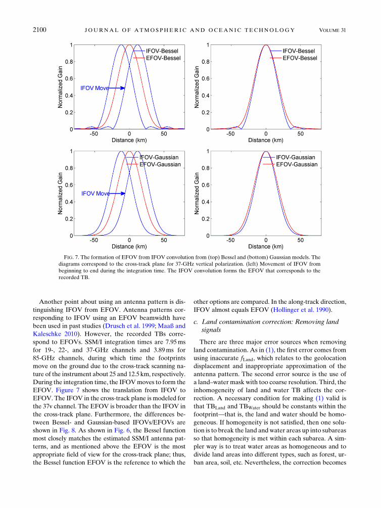
Another point about using an antenna pattern is dis-

tinguishing IFOV from EFOV. Antenna patterns cor-

responding to IFOV using an EFOV beamwidth have

been used in past studies (Drusch et al. 1999; Maaß andKaleschke 2010). However, the recorded TBs corre-

spond to EFOVs. SSM/I integration times are 7.95ms

for 19-, 22-, and 37-GHz channels and 3.89ms for

85-GHz channels, during which time the footprints

move on the ground due to the cross-track scanning na-

ture of the instrument about 25 and 12.5km, respectively.

During the integration time, the IFOVmoves to form the

EFOV. Figure 7 shows the translation from IFOV to

EFOV. The IFOV in the cross-track plane is modeled for

the 37v channel. The EFOV is broader than the IFOV in

the cross-track plane. Furthermore, the differences be-

tween Bessel- and Gaussian-based IFOVs/EFOVs are

shown in Fig. 8. As shown in Fig. 6, the Bessel function

most closely matches the estimated SSM/I antenna pat-

terns, and as mentioned above the EFOV is the most

appropriate field of view for the cross-track plane; thus,

the Bessel function EFOV is the reference to which the

other options are compared. In the along-track direction,

IFOV almost equals EFOV (Hollinger et al. 1990).

c. Land contamination correction: Removing landsignals

There are three major error sources when removing

land contamination. As in (1), the first error comes from

using inaccurate fLand, which relates to the geolocation

displacement and inappropriate approximation of the

antenna pattern. The second error source is the use of

a land–water mask with too coarse resolution. Third, the

inhomogeneity of land and water TB affects the cor-

rection. A necessary condition for making (1) valid is

that TBLand and TBWater should be constants within the

footprint—that is, the land and water should be homo-

geneous. If homogeneity is not satisfied, then one solu-

tion is to break the land andwater areas up into subareas

so that homogeneity is met within each subarea. A sim-

pler way is to treat water areas as homogeneous and to

divide land areas into different types, such as forest, ur-

ban area, soil, etc. Nevertheless, the correction becomes

FIG. 7. The formation of EFOV from IFOV convolution from (top) Bessel and (bottom) Gaussian models. The

diagrams correspond to the cross-track plane for 37-GHz vertical polarization. (left) Movement of IFOV from

beginning to end during the integration time. The IFOV convolution forms the EFOV that corresponds to the

recorded TB.


more difficult and complicated. Therefore, examining the

homogeneity, and properly modeling inhomogeneity

when necessary, is important.

Regarding land signal removal, we first consider the

strengths and limitations of previous approaches. One

option is the use of an analytical function for the cor-

rection, which assumes that the coastline is straight and

the footprint track is perpendicular to it (Desportes et al.

2007). An analytical function, including error function,

can then be used. This is computationally inexpensive.

However, the method is not sufficiently accurate in es-

timating the land signal compared to calculating the land

area (Desportes et al. 2007). Another approach is based

on calculating the land area and using the single pixel

correction (SPC) approach (Bennartz 1999; Desportes

et al. 2007; Maaß and Kaleschke 2010). SPC calculates

the area fraction of land signals and then applies a cor-

rection to each footprint/pixel one by one. Term TBLand

is estimated by selecting TB measurements with very

large values for fLand. Then, for eachmeasuredTB,TBWater

can be solved using (1). This correction strategy has the

advantage of simplicity. However, it can suffer from large

errors. The correction is vulnerable to the variation of

selected TB, because land is often more inhomo-

geneous than water and TBLand therefore has a larger

variance. Furthermore, in order to use a TB of large

land fraction, the pixel needs to be away from the coast

and thus may not well represent actual coastal TBLand.

The error in TBWater from the SPC method increases

significantly with fLand. By rearranging (1), we have

TBWater5 (TB2 fLandTBLand)/(12 fLand), where the term

1/(12 fLand) becomes very large when fLand gets close to

1, such that any small error in fLand can result in larger

errors. Thus, the SPC approach is sensitive to small er-

rors. Another previous approach is to use multiple

measurements to solve for the two unknowns, TBLand

and TBWater. The two unknowns can be solved using an

overconstrained system of equations of the form of (1).

For example, Bellerby et al. (1998) used nine pixels of

TBs to solve for TBWater. This approach has several ad-

vantages: 1) it is not necessary to directly estimate

TBLand; 2) the correction is not sensitive to the un-

certainty of a single pixel and reduces the impact of

measured TB variability; and 3) it makes use of the

spatial correlation between adjacent pixels, since either

land or water TBs with a small area are relatively ho-

mogeneous. Technically, pixels of relatively small fLandcan be used to help solve adjacent pixels of large fLand.

Two factors need to be investigated when using the

multiple pixel technique. The first is homogeneity and

spatial correlation. It is necessary to ensure that TBLand

and TBWater do not vary significantly; otherwise, it is

difficult to solve for them. The second involves choosing

an adequate number and combination of pixels, which is,

in turn, related to the first factor. Using too few pixels

makes the solution similar to that of the SPC method

and reduces its advantages. On the other hand, the ho-

mogeneity condition cannot be met when using too

FIG. 8. Antenna pattern in the cross-track plane at 37v GHz from different IFOV/EFOV assumptions. (left)

Antenna pattern for IFOV/EFOV from the Bessel and Gaussian functions, including the Gaussian pattern using

EFOV width. (right) As in (left), but with their cumulative difference with respect to the EFOV Bessel pattern.

Such differences will propagate as biases into calculating land fraction and removing land contamination.


many pixels. In particular, the number of land pixels is

important because land is more inhomogeneous and can

introduce larger errors.

We adopt the multipixel technique in our approach.

The first thing is defining a single footprint. For a single

IFOV footprint, more than 99% received power from

when Earth is within an ellipse of 3 times the 3-dB

beamwidth as shown in Fig. 5. An antenna pattern cor-

rection algorithm, including correction for spillover, has

already been applied to the TB data. Therefore, we use

this size for defining a single IFOV footprint. Further-

more, we examined the size impact by computing the land

fraction for more than 100 000 samples over Lake On-

tario in March 2006 using 3 times the 3-dB beamwidth,

where the mean is 0.7353, 0.7353, 0.7345, 0.7326, and

0.7326 for 19v, 19h, 22v, 37v, and 37h, respectively.

Modeling the antenna pattern out to 3.5 times the 3-dB

beamwidth yields mean land fractions of 0.7355, 0.7355,

0.7347, 0.7327, and 0.7327, respectively. Given a typical

land TB of 280K and a typical lake TB of 220K at 37v,

this translates to an error of 0.056K for a single pixel,

which is negligible. Thus, 3 times the 3-dB beamwidth is

adequate for a single footprint size for our land con-

tamination correction purposes.

About the number of multiple pixels, we combine

pixels within a circle with a diameter of 3 times the 3-dB

beamwidth with respect to the center pixel to remove

land contamination. This is the area from which a single

footprint receives Earth radiation. We have done both

a case study and statistical analysis to examine the im-

pact of using different sizes and numbers of pixels. (An

example illustrating the difference of using an appro-

priate number of pixels is shown in Figs. 11–13, and

statistical difference from analyzing annual data is pre-

sented in Tables 3 and 4; see below). It should be pointed

out that using multiple pixels will degrade the product

resolution. Specifically, the effective resolution is de-

graded by a factor of 3 times when using multiple pixels

within 3 times the 3-dB beamwidth. The degradation

depends on the area of the multiple pixels.

A least squares minimization method is used to esti-

mate the two unknown parameters, TBWater and TBLand,

in the multipixel approach. Using (1), each TB mea-

surement can be expressed as

TB5TBWater1 fLand(TBLand 2TBWater) . (5)

Given n . 2 measurements of TB with varying levels of

land contamination, and assuming the same values for

TBWater and TBLand in each case, (5) can be rewritten as

an overconstrained system of equations given by

y5Fx , (6)

where

y5

26664TB1

..

.

TBn

37775, F5

26664

(12 fLand)1 (fLand)1

..

.

(12 fLand)n

..

.

(fLand)n

37775, and

x5

"TBWater

TBLand

#.

(7)

The ordinary least squares (OLS) estimate for x given y

minimizes the cost function ky2Fxk2, with the solution

xOLS5 (FTF)21FTy . (8)

TheOLS solution can be overly sensitive to the presence

of outliers in the measurement vector y. In our case,

significant outliers are introduced by the presence of

rain, clouds, and inhomogeneous ground surfaces in the

measurements. Alternative regression methods, which

reduce the sensitivity to outliers, have been proposed

such as the generalized linear model (Meissner and

Wentz 2004) and robust regression (Elsaesser 2006;

Huber and Ronchetti 2009). A regression based on the

maximum likelihood estimator (MLE) was introduced

by Huber (Huber and Ronchetti 2009) and has been

developed as a form of robust regression (Elsaesser

2006; Huber andRonchetti 2009; Street et al. 1988). One

efficient computational algorithm to implement such

a regression is the iteratively reweighted least squares

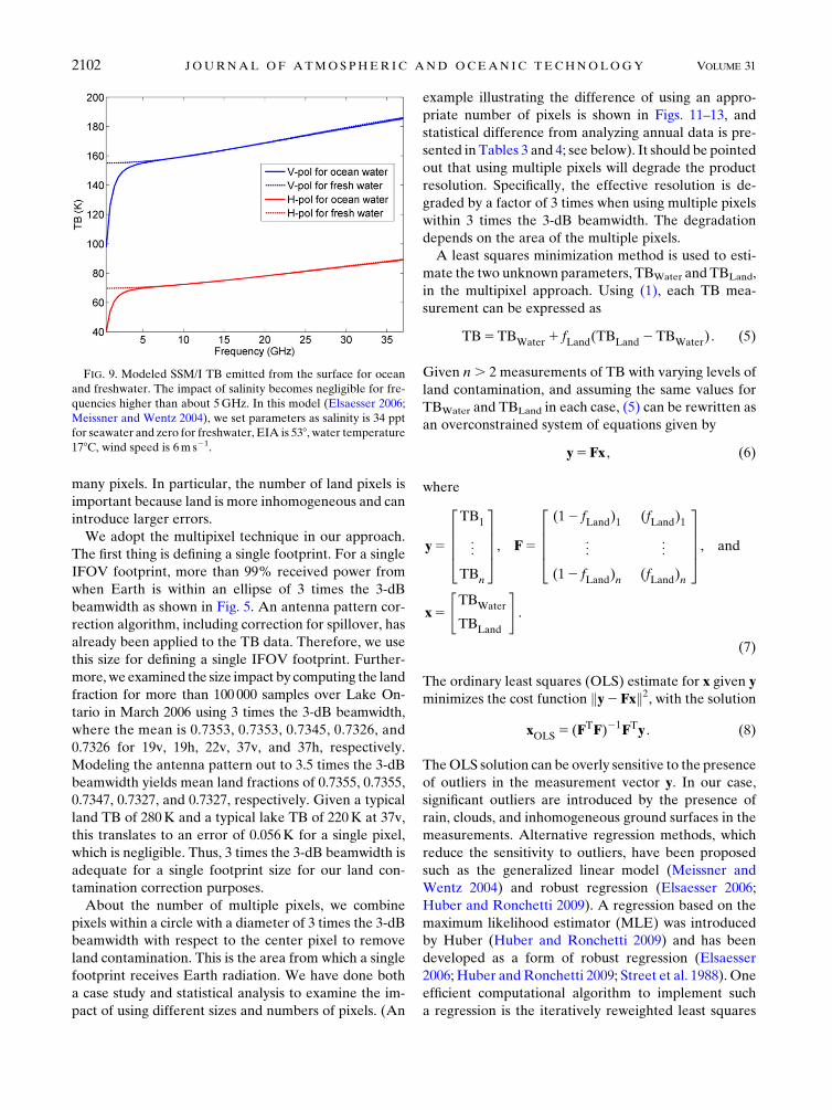
FIG. 9. Modeled SSM/I TB emitted from the surface for ocean

and freshwater. The impact of salinity becomes negligible for fre-

quencies higher than about 5GHz. In this model (Elsaesser 2006;

Meissner and Wentz 2004), we set parameters as salinity is 34 ppt

for seawater and zero for freshwater, EIA is 538, water temperature

178C, wind speed is 6m s21.


(IRLS) method (Jorgensen 2002; Street et al. 1988). We

adopt the MLE regression and implement it using the

IRLS approach. Our computational method is summa-

rized as follows.

The MLE cost function to be minimized is a weighted

version of the OLS cost function given by kW(y2Fx)k2,with solution

xMLE5 (FTWF)21FTWy , (9)

whereW is a diagonal matrix of weights. The weights are

given by

wi 5c(ri)

ri, (10)

where ri is the adjusted residual given by ri 5 (y2Fx)i/s

and s is a scale parameter. Different forms of c have

been proposed. In this study, we use the bisquare func-

tional form (Elsaesser 2006)

c(r)5

8>><>>:r

�12

r2

k2

�2, jrj# k

0, jrj. k

, (11)

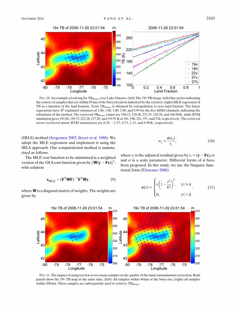
FIG. 10. An example of solving for TBWater over LakeOntario. (left) The 19v TB image, with blue circles indicating

the centers of samples that are within 95 km of the buoy (location indicated by the red dot). (right)MLE regression of

TB as a function of the land fraction. Term TBWater is obtained by extrapolation to zero land fraction. The linear

regressions have R2 explained variances of 1.00, 1.00, 1.00, 1.00, and 0.99 for the five SSM/I channels, indicating the

robustness of the method. The retrieved TBWater values are 194.13, 129.36, 221.55, 218.39, and 160.90K, while RTM

simulation gives 193.84, 130.73, 222.28, 217.26, and 159.91K at 19v, 19h, 22v, 37v, and 37h, respectively. The retrieval

errors (retrieval minus RTM simulation) are 0.29, 21.37, 0.73, 1.13, and 0.99K, respectively.

FIG. 11. The impact of using too few or toomany samples on the quality of the land contamination correction. Both

panels show the 19v TB map at the same time. (left) All samples within 40 km of the buoy site; (right) all samples

within 200 km. These samples are subsequently used to retrieve TBWater.


where k is the bounded range. The IRLS algorithm is

implemented by the following steps: 1) an initial esti-

mate is made of x using (8); 2) the weight matrix W is

computed using (10) and (11); 3) x is reestimated using

(9); and 4) steps 2 and 3 are iterated until convergence is

achieved.

In addition to the outlier measurements that are

deweighted by theMLE/IRLS approach, we also filter out

data with a large deviation from the mean. This is done by

requiring that the residual standard deviation of the linear

regression be less than 8K and that the maximum de-

viation be less than 15K. (An example of our IRLS im-

plementation is shown in Fig. 10. The difference between

using the OLS and MLE approaches is shown in Fig. 14.)

d. Retrieval algorithm implementation and resultsvalidation

After obtaining corrected TBs, existing overwater

retrieval algorithms can be applied to retrieve physical

parameters. In this study, we use data from SSM/I F-13

from 2006. The version used is provided by the recent

SSM/I fundamental climate data records (FCDR) pro-

cessed by Colorado State University (Berg et al. 2013;

Sapiano et al. 2013). The FCDR products are intercali-

brated for SSM/I sensors F-08, F-10, F-11, F-13, F-14,

and F-15 from 1987 to 2009. Each radiometer is inter-

calibrated with respect to F-13. The geolocation and

spacecraft attitude have been improvedmainly based on

FIG. 12. Retrieving TBWater using different numbers of TBs. (left) Too few TBs are used, with no warm TBs. As

a result, all TBs have corresponding land fractions less than 0.6. (right) Toomany TBs, in particular toomany warm

TBs with land fraction close to 1 (the corresponding spatial distribution of TBs can be seen in Fig. 11), are used. In

both cases, the resulting TBWater has large errors relative to the RTM simulations (shown in Fig. 13).

FIG. 13. The land contamination correction error (estimated TBWater 2 RTM-simulated TB), using different

numbers of pixels. (left) Results when using too few pixels, with no warmTBs, with correction errors of 0.34,22.33,

20.94, 1.14 and 20.40K for the five channels, respectively. (right) Results when using too many TBs, with cor-

rection errors of 1.02, 21.15, 20.08, 1.79, and 2.03K, respectively. Both cases produce worse results compared to

results using the appropriate number of pixels.


examining the coastline shift as aforementioned. No

resampling technique is applied between the different

channels.

An RTM was used to simulate contamination-free

TBs to compare with corrected TBs (Kroodsma et al.

2012). This gives a sense of the impact of the correction

within the uncertainties of the simulations. These com-

parisons are done in a relative sense, for example, Great

Lakes (land contaminated) data relative to open-ocean

data without land contamination. As such, biases in the

RTM with respect to absolute reference are not as im-

portant as capturing the functional dependence of TBs

upon variability in key geophysical parameters (wind

speed and lake surface temperature in this case). The

RTM assumes 1D parallel layers. The surface emissivity

model includes aMeissner andWentz dielectric constant

model (Meissner and Wentz 2004), a Hollinger surface

roughnessmodel (Hollinger 1971), a Stogryn foammodel

(Stogryn 1972), a Wilheit wind speed (Wilheit 1979), and

Elsaesser surface models (Elsaesser 2006). The atmo-

spheric absorption model includes Rosencrantz nitrogen

(Rosenkranz 1993) and water vapor (Rosenkranz 1998)

models, and Liebe liquid water (Liebe et al. 1991) and

oxygen models (Liebe et al. 1992). More details can be

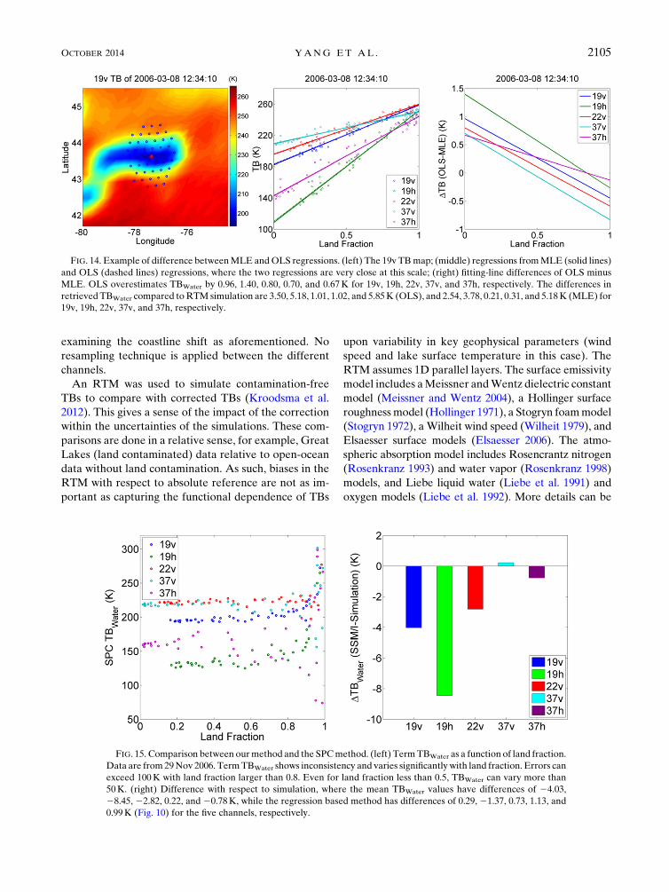
FIG. 14. Example of difference betweenMLE andOLS regressions. (left) The 19v TBmap; (middle) regressions fromMLE (solid lines)

and OLS (dashed lines) regressions, where the two regressions are very close at this scale; (right) fitting-line differences of OLS minus

MLE. OLS overestimates TBWater by 0.96, 1.40, 0.80, 0.70, and 0.67K for 19v, 19h, 22v, 37v, and 37h, respectively. The differences in

retrievedTBWater compared toRTM simulation are 3.50, 5.18, 1.01, 1.02, and 5.85K (OLS), and 2.54, 3.78, 0.21, 0.31, and 5.18K (MLE) for

19v, 19h, 22v, 37v, and 37h, respectively.

FIG. 15. Comparison between ourmethod and the SPCmethod. (left) TermTBWater as a function of land fraction.

Data are from 29Nov 2006. TermTBWater shows inconsistency and varies significantly with land fraction. Errors can

exceed 100K with land fraction larger than 0.8. Even for land fraction less than 0.5, TBWater can vary more than

50K. (right) Difference with respect to simulation, where the mean TBWater values have differences of 24.03,

28.45, 22.82, 0.22, and 20.78K, while the regression based method has differences of 0.29, 21.37, 0.73, 1.13, and

0.99K (Fig. 10) for the five channels, respectively.


found inKroodsma et al. (2012). The emissivitymodel we

use can account for salinity, where we use 34 ppt for

ocean and 0 ppt for theGreat Lakes. However, note that

the impact of salinity on water surface emissivity is most

significant for frequencies lower than 5GHz (Wilheit

1979). Figure 9 shows the impact of salinity on TB using

the emissivitymodel we use. It shows that salinity impact

is negligible above 5GHz and thus does not affect

modeling SSM/I (lowest frequency of 19.35GHz). The

input geophysical parameters for the simulation come

from the surface properties and atmosphere profiles

from 6-h Global Data Assimilation System (GDAS)

fields with a spatial resolution of 18 3 18. A land–water

mask with a resolution of about 250m (0.0020 3 0.0020)has been used (Carroll et al. 2009). Because using a high-

resolution mask increases computational expense, we

degrade this to 1 km (0.0080 3 0.0080) by averaging the

mask. Based on sensitivity studies using both original

and degraded masks to compute land fraction, the dif-

ference of degrading the land-mask resolution on the

computed TBs is of order 0.2&, which is negligible.

A regression-based wind retrieval method for the

open ocean was used (Goodberlet et al. 1989). No pa-

rameters were tuned in the wind retrieval algorithm,

because tuning the retrieval algorithm compromises its

utility for validating the robustness of a land correction.

Rain contamination was removed using a rain filter

(Stogryn et al. 1994). The retrieved wind was validated

using surface buoy measurements provided by the Na-

tionalData BuoyCenter (NDBC) (Meindl andHamilton

1992; http://www.ndbc.noaa.gov). The buoy data have

a temporal resolution of 1h. A buoy site in the center of

LakeOntario is used (43.6198N, 77.4058W). Because Lake

Ontario has the smallest surface area among the five lakes

and thus is the worst lake in terms of land-contaminated

TBs, we choose it to examine the capability of ourmethod.

This buoy site has a mean wind speed of 5.96ms21,

a maximum of 21ms21, and a variance 9.93ms21 in 2006.

The SSM/I pixel closest to the buoy site during each

overpass is used to compare with the buoy wind, and their

time difference is within 1h.

3. Results

a. Case study of removing land contamination

Figure 10 shows an example of the signal processing of

ourmethod. The left panel shows a 19vTBmapover Lake

Ontario at 2309:14 UTC 29 November 2006. Data over

LakeOntario, the smallest of theGreat Lakes, contain the

most land contamination. The red dot in the figure de-

notes the buoy site. The blue circles are centers of nearby

pixels within a circle of 190-km diameter. The right panel

shows TB as a function of fLand, which has a relationship

of TB5 fLand(TBLand 2TBWater)1TBWater. By applying

an MLE regression, TBWater is obtained at zero fLand.

The linearity between TB and fLand is quite good with an

R2 of 1.00, 1.00, 1.00, 1.00, and 0.99 for the five channels,

respectively. The retrieved values for TBWater are

194.13, 129.36, 221.55, 218.39,and 160.90K, respectively;

while RTM simulations give 193.84, 130.73, 222.28,

217.26, and 159.91K for 19v, 19h, 22v, 37v, and 37h,

respectively. The differences are 0.29, 21.37, 0.73, 1.13,

and 0.99K, respectively. The minimum fLand is approx-

imately 0.2 for channels of 19v, 19h, and 22v, indicating

that all TBs over the lake are contaminated. For chan-

nels 37v and 37h, the minimum fLand is about 0.015, be-

cause higher frequencies have smaller footprints.

Nevertheless, MLE is still found to be useful for these

FIG. 16. Comparison between using Bessel and Gaussian antenna patterns. (left) MLE regression for TBs, where filled circles and solid

lines use the Bessel pattern and unfilled circles and dashed lines use the Gaussian pattern. The data are from 29 Nov 2006. (middle)

Difference between using Bessel andGaussian patterns. (right) Term TBWater differences, which are24.32,27.07,22.10,20.90,21.77K

for the five channels, respectively. With respect to the RTM simulation, using the Gaussian pattern results in differences of24.03,28.44,

21.37, 0.23, and 20.78K, while using the Bessel pattern produces differences of 0.29, 21.37, 0.73, 1.13, and 0.99K for the five channels,

respectively. The Gaussian pattern attributes more weight to edge signals and thus removes more of the land contamination.


http://www.ndbc.noaa.gov

two channels for removal of the small amount of land

signal still present. The results show the robustness of

our method: the homogeneity in combined pixels is

satisfied, due to good geolocation, proper antenna pat-

tern, and robust regression.

The importance of using an appropriate number

of pixels to remove land contamination is examined.

Examples are illustrated in Figs. 11–13. Figure 11

maps the locations of pixels that are used to apply the

land-contamination correction. In the left panel, only

pixels within 40km of the buoy site are used, while in the

right panel, a larger number of pixels within 200km are

used. These two sets of pixels are used to retrieveTBWater.

Figure 12 shows retrievingTBWater using theMLEmethod.

The left panel corresponds to using few pixels, where

TBs have land fraction less than 0.6. The right panel

corresponds to using many pixels, where the effects of

land inhomogeneity become significant, such that the

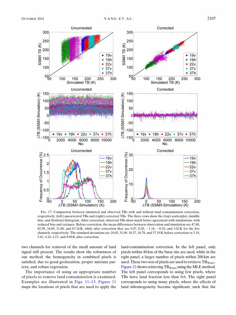
FIG. 17. Comparison between simulated and observed TBs with and without land contamination correction,

respectively: (left) uncorrected TBs and (right) corrected TBs. The three rows show the (top) scatterplot, (middle

bias, and (bottom) histogram. After correction, observed TBs show much better agreement with simulations, with

reduced bias and variance. Before correction, the mean differences between observation and simulation are 47.88,

82.99, 34.69, 31.80, and 67.16K, while after correction they are 0.47, 0.20, 21.16, 20.10, and 3.02K for the five

channels, respectively. The standard deviations are 18.05, 31.09, 16.37, 18.78, and 37.19K before correction vs 3.19,

5.81, 4.16, 4.15, and 8.69K after correction.


variance of warm TBs increases. For example, warm

TBs with a land fraction of larger than 0.98 have maxi-

mum differences of 4.16, 7.72, 3.22, 3.70, and 5.60K for

the five channels, respectively. Figure 13 shows the re-

trieved TBWater compared with simulations. In the left

panel, using few pixels has differences of 0.34, 22.33,

20.94, 1.14, and 20.40K for the five channels, re-

spectively. In the right panel, the differences are 1.02, 1.15,

0.08, 1.79, and 2.03K, respectively. Both cases produce

worse results than if the appropriate numbers of pixels is

used, as in Fig. 10, where TB differences are 0.29, 21.37,

0.73, 1.13, and 0.99K, respectively. This reduction in TB

differences demonstrates the importance of using an ap-

propriate number of pixels.

The importance of using a robust regression algorithm

is next considered. Figure 14 shows the difference

FIG. 18. TB as a function of land fraction before and after correction. (left) Before correction, TB increases signif-

icantly with land fraction. The red line from linear regression shows that TB increases by 87.05, 149.98, 67.53, 59.04, and

118.06K for the five channels, respectively, when the land fraction changes from 0 to 1. (right) After correction, TBs are

almost flat as a function of land fractionwith slopes of 2.34, 2.64, 3.27, 0.44, and 0.22K for the five channels, respectively.


between the OLS and MLE approaches. The left panel

shows a 19v TB map; the middle panel shows the MLE

(solid lines) and OLS (dashed lines) linear regressions,

which overlap in this scale but can be distinguished in

the next panel; and the right panel shows the OLSminus

MLE regressions. Compared to theMLE regression, the

OLS regression overestimates TBWater by 0.96, 1.40,

0.80, 0.70, and 0.67K for 19v, 19h, 22v, 37v, and 37h,

respectively. Their differences with respect to the RTM

simulations are 3.50, 5.18, 1.01, 1.02, and 5.85K (OLS),

and 2.54, 3.78, 0.21, 0.31, and 5.18K (MLE) for the five

channels, respectively. Measured TBs often have large

deviations in the presence of clouds and rain. The MLE

approach reduces the impact of outliers and makes the

results more consistent between channels.

b. Comparison with SPC method and Gaussianantenna pattern

Our method is compared with the SPC method in

Fig. 15. The data on 29 November 2006 were used. The

SPCmethod estimates TBLand from the TB of the highest

fLand and then calculates TBWater for each pixel. In Fig. 15,

TBWater from the SPC method shows inconsistency; that

is, TBWater varies significantly with fLand, and the errors

increase quicklywith fLand. Errors can exceed 100Kwhen

fLand is larger than 0.8. Even when fLand is less than 0.5,

TBWater varies more than 50K. With respect to the RTM

simulation, the mean TBWater has differences of 24.03,

28.45, 22.82, 0.22, and 20.78K for the five channels,

respectively. In contrast, the MLE method has differ-

ences of 0.29, 21.37, 0.73, 1.13, and 0.99K compared to

the simulations (as in Fig. 10). Therefore, the SPC

method is not practical for removing land contamination.

The importance of using the proper antenna pattern is

examined next. Figure 16 shows the difference between

using the Gaussian and Bessel antenna patterns. The

data are from 29 November 2006. The left panel shows

MLE regressions, with filled circles and solid lines from

the Bessel pattern and unfilled circles and dashed lines

from the Gaussian pattern. The middle panel shows the

FIG. 19. Comparison of (left) buoy-measured wind speed and (right) SSM/I-retrieved wind speed using (left)

corrected and (right) uncorrected TBs. Wind speed from corrected TBs shows better agreement with the buoy

measurements, with anRMSEof 1.82m s21 and a correlation of 0.86. In comparison, previous studies over the open

ocean show an RMS difference of 1.9m s21 and and R2 of 0.85 (Goodberlet et al. 1989).


fitting-line differences of Gaussian minus Bessel. The

right panel shows the TBWater differences of24.32,27.07,

22.10, 20.90, and21.77K for the five channels, re-

spectively. With respect to RTM simulation, using the

Gaussian pattern shows differences of 24.03, 28.44,

21.37, 0.23, and 20.78K, while the Bessel pattern shows

differences of 0.29, 21.37, 0.73, 1.13, and 0.99K for the

five channels, respectively. The Gaussian pattern attri-

butes more weight to edge signals and thus removes more

signals. The Gaussian pattern does not approximate the

antenna pattern as well and, as a result, produces much

larger errors.

c. Validation of contamination-free TB and retrievedwind speed

The corrected TBWater is compared with simulated

TBs to test for physical reasonableness. Figure 17 shows

the comparison between observed and measured TB for

annual data over all of Lake Ontario. There are 10 936

samples for each channel. Measured raw TBs are overall

warmer than the simulated values before correction (left

side). After correction (right side), the simulated and

measured TBs are well aligned in the 1-to-1 solid line

(top plot). Both the bias (middle plot) and variance

(bottom plot) are reduced. Before correction, TBs are

warmer with respect to the simulation by 47.88, 82.99,

34.69, 31.80, and 67.16K, while after correction the dif-

ferences are 0.47, 0.20, 21.16, 20.10, and 3.02K for the

five channels, respectively. The standard deviations are

18.05, 31.09, 16.37, 18.78, and 37.19K before correction

versus 3.19, 5.81, 4.16, 4.15, and 8.69K after correction

for the five channels, respectively. The 37h channel

shows a larger difference, but the exact reason for this is

not known. According to the standard deviation, the

residual differences are about 4K.However, it should be

pointed out that the residual error in our correction

method is much less, because part of the difference

comes from uncertainties in the simulated TBs. The

error analysis shown in the following section, based on

comparisons between wind retrievals and ground truth

winds, shows much smaller residual errors.

Figure 18 shows TBs as a function of land fraction

before and after correction. Before correction, TBs in-

crease with land fraction. The fitted red line from a lin-

ear regression shows that TBs increase by 87.05, 149.98,

67.53, 59.04, and 118.06K for the five channels, re-

spectively, when land fractions change from 0 to 1. After

correction, TBs have only a small dependence on land

fraction. The slope becomes 2.34, 2.64, 3.27, 0.44, and

0.22K for the five channels, respectively.

It should be noted that comparisons to simulations is

not the absolute benchmark for validation. To charac-

terize the magnitude of any simulation biases, TBs were

simulated over land-free ocean using the RTM and

GDAS profiles and were compared to observations. The

comparison was implemented over latitudes of 4082508in the Northern Hemisphere; these latitudes are similar

to that of the Great Lakes. The simulated and observed

data were averaged into 18 3 18 grid boxes and com-

pared. Data with cloud liquid water are eliminated to

isolate just surface effects, which are the most relevant

to the retrieval of wind speeds. Furthermore, it should

be noted that the middle of ocean has sparse in situ

observations that limit the accuracy of GDAS atmo-

spheric profiles. Data with large spatial inhomogeneity

are filtered out, that is, TBs in the same 18 3 18 grid box

TABLE 1. Comparison of corrected TB against simulation using different antenna patterns. Bias is raw/corrected TB minus simulated

TB.G-IFOV is using aGaussian function–based IFOV antenna pattern, where SSM/I EFOVwidths are the input parameters. G-EFOV is

using a Gaussian function–based EFOV. B-IFOV is using a Bessel function–based IFOV antenna pattern. B-EFOV is using a Bessel

function–based EFOV. Method B-EFOV gives overall the best results with small bias and standard deviation.

TB

Raw G-IFOV G-EFOV B-IFOV B-EFOV Open ocean

Bias STD Bias STD Bias STD Bias STD Bias STD Bias STD

19v 47.88 18.05 20.51 3.20 21.05 3.23 1.01 3.15 0.47 3.19 1.10 2.97

19h 82.99 31.09 21.53 5.76 22.42 5.85 1.17 5.70 0.20 5.81 0.47 5.54

22v 34.69 16.37 21.56 4.20 22.02 4.23 20.68 4.12 21.16 4.16 0.73 4.93

37v 31.80 18.78 0.25 4.08 20.32 4.14 0.51 4.10 20.10 4.15 22.79 3.57

37h 67.16 37.19 3.74 8.51 2.57 8.68 4.26 8.54 3.02 8.69 20.62 7.67

TABLE 2. Comparison of wind speed retrieval against buoy using different antenna patterns. Terms as in Table 1. B-EFOV gives overall

the best results with large correlation and small RMSE. The numbers for the open ocean are from Goodberlet et al. (1989).

Raw G-IFOV G-EFOV B-IFOV B-EFOV Open ocean

R2 RMSE R2 RMSE R2 RMSE R2 RMSE R2 RMSE R2 RMSE

0.71 2.86 0.83 1.97 0.84 1.93 0.85 1.86 0.86 1.82 0.85 1.90


with a standard deviation larger than 2K at each chan-

nel. The TB differences (observation minus simulation)

are 1.10, 0.47, 0.73, 22.79, and 20.62K for the five

channels, respectively. The standard deviations of TB

differences are 2.97, 5.54, 4.93, 3.57, and 7.67K for the

five channels, respectively. This residual error in the

open ocean falls into the same order as the land-

corrected TBs over the Lake Ontario.

The corrected values for TBWater over Lake Ontario

were used for wind speed retrieval and were validated

against surface buoymeasurements. Figure 19 shows the

comparison between buoy and SSM/I retrieved wind

speeds. The coincidence data are within 1 h, during

which the hourly buoy wind is compare with SSM/I wind

from the closest pixel to the buoy. By using the corrected

TB, the SSM/I wind speed retrieval is significantly im-

proved, with smaller bias and variance and enhanced

correlation. The root-mean-square error (RMSE) is

1.82m s21 and the correlation is 0.86. Over the open

ocean, previous studies reported an RMSE of 1.9m s21

and a correlation of 0.85 when comparing buoy and

SSM/I wind speeds (Goodberlet et al. 1989). Note that

the retrieved wind speed still has some residual bias and

some negative values. This is partly because the retrieval

algorithm used here was specifically tuned for the open

ocean. Figure 19 has fewer data points than Fig. 18,

because the buoy site has limited data where no data are

available in winter and SSM/I passes the same place only

2 times per day. We use the residual error in the wind

retrievals to estimate the error in the corrected TBs. As

an approximation to bound the TB uncertainties, it is

assumed that the standard deviation of the TB residual

error is equivalent at each channel and that the co-

variance of any two channels is zero. Then the standard

deviation of the TB residual error can be derived from

the standard deviation of the wind residual error as

s2Wind5 �

ia2i s

2TBi 5s2

TB�ia2i , (12)

where ai denotes constant parameters in the regression-

based wind algorithm. The standard deviation of the

wind speed residual error is sWind 5 1:86m s21, and

therefore the corresponding standard deviation of TB is

obtained as sTB 5 0:80 K for each channel.

We note that there are more state-of-the-art wind

retrieval algorithms than the one used here. However,

the point in this study is to demonstrate the impact of the

land contamination on an example product derived from

the corrected TBs, not to produce the most accurate

wind speed retrievals. We will study those algorithms

and combine different radiometers to produce climato-

logical wind products over the Great Lakes in future

work, where it is expected that the improved spatial

coverage from multiple satellites will yield valuable in-

formation on the cross-lake distributions relative to

buoy data alone.

The comparisons between using different antenna

patterns are presented in Tables 1 and 2. The two tables

come from analyzing the same data in 2006 using differ-

ent antenna patterns. Table 1 presents the comparison

between raw/corrected TBs and simulated TBs, using

Bessel-/Gaussian-based IFOV and EFOV antenna

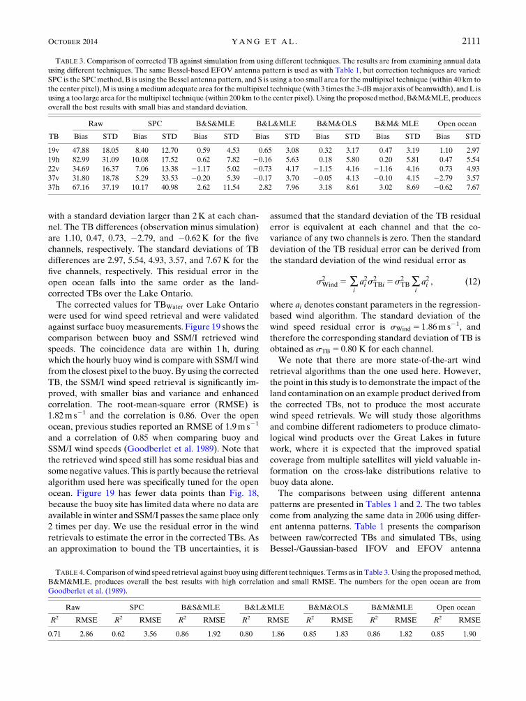
TABLE 3. Comparison of corrected TB against simulation from using different techniques. The results are from examining annual data

using different techniques. The same Bessel-based EFOV antenna pattern is used as with Table 1, but correction techniques are varied:

SPC is the SPCmethod, B is using the Bessel antenna pattern, and S is using a too small area for the multipixel technique (within 40 km to

the center pixel),M is using amedium adequate area for themultipixel technique (with 3 times the 3-dBmajor axis of beamwidth), andL is

using a too large area for themultipixel technique (within 200 km to the center pixel). Using the proposedmethod, B&M&MLE, produces

overall the best results with small bias and standard deviation.

TB

Raw SPC B&S&MLE B&L&MLE B&M&OLS B&M& MLE Open ocean

Bias STD Bias STD Bias STD Bias STD Bias STD Bias STD Bias STD

19v 47.88 18.05 8.40 12.70 0.59 4.53 0.65 3.08 0.32 3.17 0.47 3.19 1.10 2.97

19h 82.99 31.09 10.08 17.52 0.62 7.82 20.16 5.63 0.18 5.80 0.20 5.81 0.47 5.54

22v 34.69 16.37 7.06 13.38 21.17 5.02 20.73 4.17 21.15 4.16 21.16 4.16 0.73 4.93

37v 31.80 18.78 5.29 33.53 20.20 5.39 20.17 3.70 20.05 4.13 20.10 4.15 22.79 3.57

37h 67.16 37.19 10.17 40.98 2.62 11.54 2.82 7.96 3.18 8.61 3.02 8.69 20.62 7.67

TABLE 4. Comparison of wind speed retrieval against buoy using different techniques. Terms as in Table 3. Using the proposedmethod,

B&M&MLE, produces overall the best results with high correlation and small RMSE. The numbers for the open ocean are from

Goodberlet et al. (1989).

Raw SPC B&S&MLE B&L&MLE B&M&OLS B&M&MLE Open ocean

R2 RMSE R2 RMSE R2 RMSE R2 RMSE R2 RMSE R2 RMSE R2 RMSE

0.71 2.86 0.62 3.56 0.86 1.92 0.80 1.86 0.85 1.83 0.86 1.82 0.85 1.90


patterns. The bias is the mean residual of raw/corrected

TB minus simulated TB, and the standard deviation

(STD) of the residual is also shown. Overall, using the

Bessel-based EFOV antenna pattern produces the best

results with the smallest bias and standard deviation.

Table 2 shows the retrieved wind speed against buoy.

Again, the proposed method provides the best wind

retrieval against buoy measurements with high correla-

tion and small RMSE.

The comparisons between different correction tech-

niques are shown in Tables 3 and 4. The same Bessel-

based antenna pattern is used, but different correction

techniques in the aforementioned case study are used to

examine all data in 2006 and then results are compared.

These different techniques include SPC compared to

multipixel, OLS compared to MLE, and using an in-

adequate number of pixels in the retrieval method com-

pared to using adequate pixels. Table 3 shows the

comparison of correctedTBagainst simulation, andTable

4 presents wind retrieval against buoy. Overall, our pro-

posed method (i.e., Bessel-based EFOV antenna pattern,

multiple pixel method with adequate number combina-

tion, andMLE regression) produces TBs andwind speeds

with the lowest bias and standard deviation/RMSE with

respect to simulated TBs and buoy winds, respectively.

4. Conclusions

We have examined methods for correcting land con-

tamination of passive radiometer measurements in or-

der to extract coastal and inland lake information. The

method presented in the paper significantly reduces

the land contamination, and the corrected TBs show

agreement with simulations. The corrected data are

used for wind retrieval over the Great Lakes. Our land

contamination algorithm uses a Bessel function–based

representation of the EFOV antenna pattern, combines

an appropriate number of neighboring samples, and uses

the maximum likelihood estimator (MLE) regression to

remove land contamination. We compare our method

with previous approaches and examine the difference

between using different techniques. It is found that using

an appropriate antenna pattern is important for re-

moving land contamination, and that the Bessel pattern

outperforms the Gaussian pattern. The results are much

better compared to techniques based on a single pixel

correction. However, it should be noted that the reso-

lution is degraded. The example retrievals show im-

proved wind speed with an RMS error of 1.86m s21. By

using this method, the current lack of information near

coasts in standard SSM/I data products can be ad-

dressed. This method can be applied to other radiome-

ters in coastal regions for general retrieval purposes.

Acknowledgments. The authors thank Colorado State

University for providing the SSM/I Fundamental Cli-

mate Data Record (FCDR). We thank the anonymous

reviewers for their useful comments.

REFERENCES

Bellerby, T., M. Taberner, A.Wilmshurst,M. Beaumont, E. Barrett,

J. Scott, and C. Durbin, 1998: Retrieval of land and sea

brightness temperatures from mixed coastal pixels in passive

microwave data. IEEE Trans. Geosci. Remote Sens., 36, 1844–

1851, doi:10.1109/36.729355.

Bennartz, R., 1999: On the use of SSM/I measurements in coastal

regions. J. Atmos. Oceanic Technol., 16, 417–431, doi:10.1175/

1520-0426(1999)016,0417:OTUOSI.2.0.CO;2.

Berg, W., M. R. P. Sapiano, J. Horsman, and C. Kummerow, 2013:

Improved geolocation and Earth incidence angle information

for a fundamental climate data record of the SSM/I sensors.

IEEE Trans. Geosci. Remote Sens., 51, 1504–1513, doi:10.1109/

TGRS.2012.2199761.

Carroll, M. L., J. R. Townshend, C. M. DiMiceli, P. Noojipady, and

R. A. Sohlberg, 2009: A new global raster water mask at 250m

resolution. Int. J. Digital Earth, 2, 291–308, doi:10.1080/

17538940902951401.

Colton, M. C., and G. A. Poe, 1999: Intersensor calibration of

DMSP SSM/I’s: F-8 to F-14, 1987-1997. IEEE Trans. Geosci.

Remote Sens., 37, 418–439, doi:10.1109/36.739079.Desportes, C., E. Obligis, and L. Eymard, 2007: On the wet tro-

pospheric correction for altimetry in coastal regions. IEEE

Trans. Geosci. Remote Sens., 45, 2139–2149, doi:10.1109/

TGRS.2006.888967.

Drusch,M., E. F.Wood, andR.Lindau, 1999: The impact of theSSM/I

antenna gain function on land surface parameter retrieval. Geo-

phys. Res. Lett., 26, 3481–3484, doi:10.1029/1999GL010492.

Elsaesser, G., 2006: A parametric optimal estimation retrieval of

the non-precipitating parameters over the global oceans. M.S.

thesis, Dept. of Atmospheric Science, Colorado State Uni-

versity, 87 pp.

Galindo-Israel, V., andR.Mittra, 1977:A new series representation

for the radiation integral with application to reflector antennas.

IEEE Trans. Antennas Propag., 25, 631–641, doi:10.1109/

TAP.1977.1141657.

Goodberlet, M. A., C. T. Swift, and J. C. Wilkerson, 1989: Remote

sensing of ocean surface winds with the Special Sensor Micro-

wave Imager. J. Geophys. Res., 94, 14 547–14 555, doi:10.1029/

JC094iC10p14547.

Hollinger, J. P., 1971: Passive microwave measurements of sea

surface roughness. IEEE Trans. Geosci. Electron., 9, 165–169,

doi:10.1109/TGE.1971.271489.

——, J. L. Peirce, and G. A. Poe, 1990: SSM/I instrument evalua-

tion. IEEE Trans. Geosci. Remote Sens., 28, 781–790,

doi:10.1109/36.58964.

Huber, P. J., and E. M. Ronchetti, 2009: Robust Statistics. 2nd ed.

Wiley Series in Probability and Statistics, John Wiley, 380 pp.

Hung, C. C., and R. Mittra, 1983: Secondary pattern and focal re-

gion distribution of reflector antennas under wide-angle scan-

ning. IEEE Trans. Antennas Propag., 31, 756–763, doi:10.1109/

TAP.1983.1143141.

Jorgensen,M., 2002: Iteratively reweighted least squares.Encyclopedia

of Environmetrics, A. H. El-Shaarawi and W. W. Piegorsch,

Eds., John Wiley & Sons, Ltd., 1084–1088.


http://dx.doi.org/10.1109/36.729355

http://dx.doi.org/10.1175/1520-0426(1999)016<0417:OTUOSI>2.0.CO;2

http://dx.doi.org/10.1175/1520-0426(1999)016<0417:OTUOSI>2.0.CO;2

http://dx.doi.org/10.1109/TGRS.2012.2199761


http://dx.doi.org/10.1080/17538940902951401

http://dx.doi.org/10.1080/17538940902951401

http://dx.doi.org/10.1109/36.739079



http://dx.doi.org/10.1029/1999GL010492

http://dx.doi.org/10.1109/TAP.1977.1141657


http://dx.doi.org/10.1029/JC094iC10p14547

http://dx.doi.org/10.1029/JC094iC10p14547

http://dx.doi.org/10.1109/TGE.1971.271489

http://dx.doi.org/10.1109/36.58964



Kroodsma, R. A., D. S. McKague, and C. S. Ruf, 2012: Inter-

calibration of microwave radiometers using the vicarious

cold calibration double difference method. IEEE J. Sel. Top.

Appl. Earth Obs. Remote Sens., 5, 1006–1013, doi:10.1109/JSTARS.2012.2195773.

Liebe, H. J., G. A. Hufford, and T. Manabe, 1991: A model for the

complex permittivity of water at frequencies below 1THz. Int.

J. Infrared Millimeter Waves, 12, 659–675, doi:10.1007/

BF01008897.

——, P. W. Rosenkranz, and G. A. Hufford, 1992: Atmospheric

60-GHz oxygen spectrum: New laboratory measurements and

line parameters. J. Quant. Spectrosc. Radiat. Transfer, 48, 629–643, doi:10.1016/0022-4073(92)90127-P.

Maaß, N., and L. Kaleschke, 2010: Improving passive microwave

sea ice concentration algorithms for coastal areas: Applica-

tions to the Baltic Sea. Tellus, 62A, 393–410, doi:10.1111/

j.1600-0870.2010.00452.x.

Meindl, E. A., andG. D. Hamilton, 1992: Programs of the National

Data Buoy Center. Bull. Amer. Meteor. Soc., 73, 985–993,doi:10.1175/1520-0477(1992)073,0985:POTNDB.2.0.CO;2.

Meissner, T., and F. J. Wentz, 2004: The complex dielectric con-

stant of pure and sea water from microwave satellite obser-

vations. IEEE Trans. Geosci. Remote Sens., 42, 1836–1849,doi:10.1109/TGRS.2004.831888.

Mittra, R., Y. Rahmat-Samii, V. Galindo-Israel, and R. Norman,

1979: An efficient technique for the computation of vector

secondary patterns of offset paraboloid reflectors. IEEE Trans.

Antennas Propag., 27, 294–304, doi:10.1109/TAP.1979.1142086.

Poe, G. A., and R. W. Conway, 1990: A study of the geolocation

errors of the Special Sensor Microwave Imager (SSM/I). IEEE

Trans. Geosci. Remote Sens., 28, 791–799, doi:10.1109/36.58965.

Rahmat-Samii, Y., and V. Galindo-Israel, 1980: Shaped reflector

antenna analysis using the Jacobi-Bessel series. IEEE

Trans. Antennas Propag., 28, 425–435, doi:10.1109/

TAP.1980.1142364.

Rosenkranz, P. W., 1993: Absorption of microwaves by atmo-

spheric gases. Atmospheric Remote Sensing by Microwave

Radiometry, M. A. Janssen, Ed., John Wiley, 37–90.

——, 1998: Water vapor microwave continuum absorption: A

comparison of measurements and models.Radio Sci., 33, 919–

928, doi:10.1029/98RS01182.

Sapiano,M.R. P.,W.K.Berg,D. S.McKague, andC.D.Kummerow,

2013: Toward an intercalibrated fundamental climate data re-

cord of the SSM/I sensors. IEEETrans.Geosci. Remote Sens., 51,

1492–1503, doi:10.1109/TGRS.2012.2206601.

Stogryn, A. P., 1972: The emissivity of sea foam at microwave

frequencies. J. Geophys. Res., 77, 1658–1666, doi:10.1029/

JC077i009p01658.

——, C. T. Butler, and T. J. Bartolac, 1994: Ocean surface wind

retrievals from Special Sensor Microwave Imager data with

neural networks. J. Geophys. Res., 99, 981–984, doi:10.1029/

93JC03042.

Street, J. O., R. J. Carroll, and D. Ruppert, 1988: A note on com-

puting robust regression estimates via iteratively reweighted

least squares. Amer. Stat., 42, 152–154.

Ulaby, F. T., and D. G. Long, 2014: Microwave Radar and Ra-

diometric Remote Sensing. University of Michigan Press,

1016 pp.

Wilheit, T. T., 1979: A model for the microwave emissivity of

the ocean’s surface as a function of wind speed. IEEE

Trans. Geosci. Remote Sens., 17, 244–249, doi:10.1109/

TGE.1979.294653.


http://dx.doi.org/10.1109/JSTARS.2012.2195773

http://dx.doi.org/10.1109/JSTARS.2012.2195773

http://dx.doi.org/10.1007/BF01008897

http://dx.doi.org/10.1007/BF01008897

http://dx.doi.org/10.1016/0022-4073(92)90127-P

http://dx.doi.org/10.1111/j.1600-0870.2010.00452.x

http://dx.doi.org/10.1111/j.1600-0870.2010.00452.x

http://dx.doi.org/10.1175/1520-0477(1992)073<0985:POTNDB>2.0.CO;2



http://dx.doi.org/10.1109/36.58965



http://dx.doi.org/10.1029/98RS01182


http://dx.doi.org/10.1029/JC077i009p01658

http://dx.doi.org/10.1029/JC077i009p01658

http://dx.doi.org/10.1029/93JC03042

http://dx.doi.org/10.1029/93JC03042



land contamination correction for passive...

Documents