lampiran a hasil pengamatan standarisasi …repository.wima.ac.id/727/7/lampiran.pdf · hasil...

103

LAMPIRAN A

HASIL PENGAMATAN STANDARISASI PARAMETER SPESIFIK DAN NON SPESIFIK EKSTRAK TOMAT (Lycopersicum esculentum

Mill.)

A. Standarisasi parameter spesifik ekstrak tomat

Tabel 4.22. Pemeriksaan organoleptis ekstrak tomat

Pemeriksaan Ekstrak tomat Bentuk Serbuk Warna Jingga Muda

Bau Khas aromatik

Tabel 4.23. Hasil pemeriksaan sifat fisik penentuan pH ekstrak tomat Replikasi Ekstrak tomat

1 5,06 2 4,97 3 4,91

X ± SD 4,98 ± 0,0755

104

Tabel 4.24. Hasil penentuan ukuran partikel ekstrak tomat

Replikasi No. mesh

d (µm)

Ln d (µm)

Berat ekstrak

yang tertahan

(g)

% bobo

t

% FKB

Nilai Z

1 20 850 6,7452 0,16 0,16 99,99 3,49 40 425 6,0529 0,49 0,49 99,5 2,58 60 250 5,5215 2,67 2,67 96,83 1,86 80 180 5,1930 1,55 1,55 95,28 1,67 100 150 5,0106 0,86 0,86 94,42 1,59 120 125 4,8283 2,34 2,34 92,08 1,41 Pan 0 92,08 92,08 0 -3,49 ∑ 100,15

2 20 850 6,7452 0,76 0,76 99,26 2,43 40 425 6,0529 2,87 2,87 96,39 1,80 60 250 5,5215 4,77 4,77 91,62 1,38 80 180 5,1930 6,05 6,05 85,57 1,06 100 150 5,0106 1,27 1,27 84,3 1,01 120 125 4,8283 1,03 1,03 83,27 0,96 Pan 0 83,27 83,27 0 -3,49 ∑ 100,02

3 20 850 6,7452 0,07 0,07 99,94 3,22 40 425 6,0529 0,19 0,19 99,75 2,81 60 250 5,5215 1,12 1,12 98,63 2,21 80 180 5,1930 0,71 0,71 97,92 2,04 100 150 5,0106 0,18 0,18 97,74 2,00 120 125 4,8283 0,38 0,38 97,36 1,94 Pan 0 97,36 97,54 0 -3,49 ∑ 100,01

Replikasi d 50% d 84% σg dvs 1 32,4370 87,0863 2,6848 0,628 2 50,7545 158,4279 3,1214 0,7605 3 26,2299 69,6791 2,5817 0,553

105

Contoh cara perhitungan :

Log dvs = log dg (50%) – 1,151 log2 σg

= log 32,4370 – 1,151 log2 2,6848

= 1,5110 – 0,883

= 0,628 µm

106

Tabel 4.25. Hasil uji kadar sari larut air ekstrak tomat

Replikasi Berat cawan

(g)

Berat ekstrak

(g)

Berat konstan atau yang sudah

dipanaskan (g)

% kadar

1 42,6185 5,1 43,4594 16,49 2 44,6530 5,0 45,4743 16,43 3 33,1482 5,0 34,0092 17,22 X

± SD 16,71

± 0,4416 Contoh cara perhitungan :

Berat konstan atau yang sudah dipanaskan – berat cawan x 100%

Berat ekstrak

43,4594 – 42,6185 x 100%

5,1

Tabel 4.26. Hasil uji kadar sari larut alkohol ekstrak tomat

Replikasi Berat cawan (g)

Berat ekstrak

(g)

Berat konstan atau yang sudah dipanaskan (g)

% kadar

1 47,0310 5,0 47,0618 0,616 2 41,9821 5,0 42,0258 0,874 3 40,0726 5,0 40,1206 0,96

X ± SD 0,8167 ± 0,179


Berat konstan atau yang sudah dipanaskan – berat cawan x 100%

Berat ekstrak

47,0618 – 47,0310 x 100%

5,0

=

= 16,49 %

= 0,616 %

=

107

B. Standarisasi parameter spesifik ekstrak tomat

Tabel 4.27. Hasil pemeriksaan uji susut pengeringan ekstrak tomat

Replikasi Ekstrak tomat 1 4,3 2 4,1 3 4,2

X ± SD 4,2 ± 0,1

Tabel 4.28. Hasil uji kadar air ekstrak tomat

Replikasi Berat cawan

(g)

Berat cawan +

ekstrak (g)

Berat cawan + ekstrak

konstan (g)

% kadar

1 50,6014 60,6052 60,3599 0,4047 2 57,9935 67,9995 67,7464 0,3722 3 50,0131 60,0318 59,7767 0,4249

X ± SD 0,4006 ± 0,0266


(Berat cawan + ekstrak) – (berat cawan + ekstrak konstan) x 100%

Berat cawan + ekstrak

60,6052- 60,3599 x 100%

60,6052

Tabel 4.29. Hasil uji kadar abu total ekstrak tomat

Replikasi Berat krus (g)

Berat ekstrak (g)

Berat krus + abu konstan (g)

% kadar

1 22,3168 2,5113 22,3312 0,57 2 21,8919 2,5184 21,9075 0,62 3 23,3719 2,5149 23,3916 0,78

X ± SD 0,66 ± 0,1103

=

= 0,4047%

108


(Berat krus + abu konstan) – berat krus x 100%

Berat ekstrak

22,3312 – 22,3168 x 100%

2,5113

Tabel 4.30. Hasil uji kadar abu tidak larut asam ekstrak tomat

Replikasi Berat krus (g)

Berat krus + abu (g)

Berat abu + HCl

konstan (g)

% kadar

1 22,3168 22,3312 23,3172 2,78 2 21,8920 21,9063 21,8925 3,49 3 23,3717 23,3860 23,3721 2,79

X ± SD 3,02 ± 0,4112


( Berat abu + HCl konstan) – berat krus x 100%

(Berat krus + abu) - berat krus

23,3172 – 22,3168 x 100%

22,3312 – 22,3168

Tabel 4.31. Hasil uji kadar abu larut air ekstrak tomat

Replikasi

Berat krus (g)

Berat krus + abu konstan (g)

Berat abu + aquades

(g)

% kadar

1 34,4410 34,4604 34,4414 2,04 2 36,2150 36,2347 36,2156 3,04 3 35,9810 36,0098 35,9818 2,78

X ± SD 2,62 ± 0,52

=

= 0,57 %

=

= 2,78 %

109


Berat abu setelah penambahan aquades-berat krus x 100%

(Berat krus + abu) - berat krus

34,4414 – 34,4410 x 100%

34,4604 – 34,4410

=

= 2,04%

110

LAMPIRAN B

HASIL PERHITUNGAN LARUTAN PENYALUT TABLET SALUT ENTERIK EKSTRAK TOMAT

Contoh hasil perhitungan larutan penyalut :

Jumlah tablet inti : 350 tablet

Jumlah total tablet inti : 141,2 gram

Jumlah HPMCP (dengan penambahan bobot 4%) :

4/100 x 141,2 = 5,648 gram

Volume pelarut campur dengan konsentrasi HPMCP 5% :

100/5 x 5,648 = 112,96 ml

Jumlah plastisaiser 0,5% : 0,5/100 x 5,648 = 0,02824 gram

Jumlah talk 4% : 4/100 x 141,2 = 0,2259 gram

% pelarut campuran : 112,96 – (5,648 + 0,02824) + 0,2259 = 107,054 ml

111

LAMPIRAN C

HASIL PERHITUNGAN PERBANDINGAN PENGISI PADA EKSTRAK TOMAT

Contoh hasil perhitungan :

Rasio ekstrak : pengisi = 2,8 : 1

Pengisi : Maltodextrin

Dosis ekstrak untuk tiap tablet : 250 mg

Ekstrak yang harus ditimbang : 3,8/2,8 x 250 = 339,29 mg/tablet

112

LAMPIRAN D

HASIL UJI STATISTIK MUTU FISIK LARUTAN PENYALUT ANTAR FORMULA TABLET SALUT ENTERIK EKSTRAK

TOMAT

A. Uji Viskositas Larutan Penyalut

ANOVA

Viskositas

Sum of Squares Df Mean Square F Sig.

Between Groups

30314.750 3 10104.917 21809.173 .000

Within Groups 3.707 8 .463

Total 30318.457 11

Post Hoc Tests

Multiple Comparisons

Tukey HSD

(I) formula

(J) formula

Mean Difference

(I-J) Std.

Error Sig.

95% Confidence Interval

Lower Bound

Upper Bound

Fa fb -114.63333* .55578 .000 -116.4131 -112.8535

fc 1.46667 .55578 .111 -.3131 3.2465

fd -78.23333* .55578 .000 -80.0131 -76.4535

Fb fa 114.63333* .55578 .000 112.8535 116.4131

fc 116.10000* .55578 .000 114.3202 117.8798

113

fd 36.40000* .55578 .000 34.6202 38.1798

fc fa -1.46667 .55578 .111 -3.2465 .3131

fb -116.10000* .55578 .000 -117.8798 -114.3202

fd -79.70000* .55578 .000 -81.4798 -77.9202

fd fa 78.23333* .55578 .000 76.4535 80.0131

fb -36.40000* .55578 .000 -38.1798 -34.6202

fc 79.70000* .55578 .000 77.9202 81.4798

*. The mean difference is significant at the 0.05 level. F hitung (21809,173) > F0,05 (3,8) = 4,07 sehingga ada perbedaan bermakna antar formula Homogeneous Subsets

Viskositas

Tukey HSDa

formula N

Subset for alpha = 0.05

1 2 3

fc 3 22.9000

fa 3 24.3667

fd 3 102.6000

fb 3 139.0000

Sig. .111 1.000 1.000

Means for groups in homogeneous subsets are displayed.

a. Uses Harmonic Mean Sample Size = 3.000.

114

B. Uji Berat Jenis Larutan Penyalut

ANOVA

Berat Jenis Sum of

Squares Df Mean Square F Sig.

Between Groups

.001 3 .000 14.202 .001

Within Groups .000 8 .000

Total .001 11

Post Hoc Tests


Tukey HSD

(I) formula

(J) formula

Mean Difference

(I-J) Std.

Error Sig.


Lower Bound

Upper Bound

fa fb -.02097* .00426 .005 -.0346 -.0073

fc .00513 .00426 .641 -.0085 .0188

fd -.00277 .00426 .913 -.0164 .0109

fb fa .02097* .00426 .005 .0073 .0346

fc .02610* .00426 .001 .0124 .0398

fd .01820* .00426 .012 .0045 .0319

fc fa -.00513 .00426 .641 -.0188 .0085

115

fb -.02610* .00426 .001 -.0398 -.0124

fd -.00790 .00426 .318 -.0216 .0058

Fd fa .00277 .00426 .913 -.0109 .0164

fb -.01820* .00426 .012 -.0319 -.0045

fc .00790 .00426 .318 -.0058 .0216

*. The mean difference is significant at the 0.05 level. F hitung (14,202) > F0,05 (3,8) = 4,07 sehingga ada perbedaan bermakna antar formula Homogeneous Subsets

Berat Jenis

Tukey HSDa

formula N


1 2

Fc 3 1.0134

Fa 3 1.0185

Fd 3 1.0213

Fb 3 1.0395

Sig. .318 1.000



116

C. UJI pH Larutan Penyalut

ANOVA

pH Larutan Penyalut Sum of

Squares Df Mean Square F Sig.

Between Groups

.273 3 .091 1363.458 .000

Within Groups .001 8 .000

Total .273 11

Post Hoc Tests


Tukey HSD

(I) formula

(J) formula

Mean Difference

(I-J) Std.

Error Sig.


Lower Bound

Upper Bound

Fa fb .28667* .00667 .000 .2653 .3080

fc -.07000* .00667 .000 -.0913 -.0487

fd .23333* .00667 .000 .2120 .2547

Fb fa -.28667* .00667 .000 -.3080 -.2653

fc -.35667* .00667 .000 -.3780 -.3353

fd -.05333* .00667 .000 -.0747 -.0320

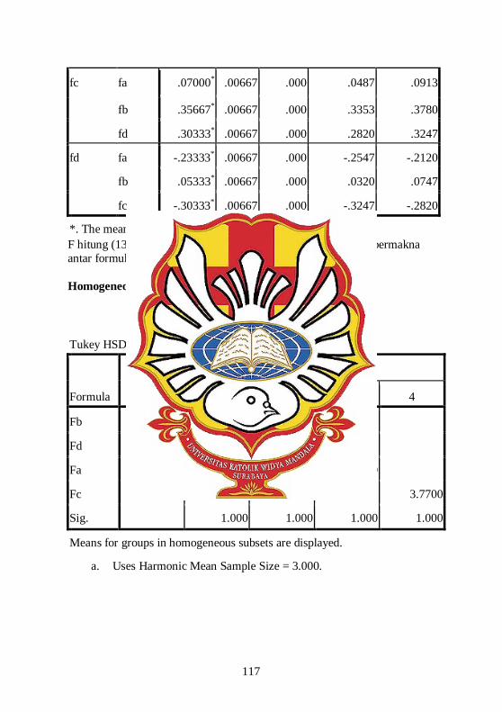
117

fc fa .07000* .00667 .000 .0487 .0913

fb .35667* .00667 .000 .3353 .3780

fd .30333* .00667 .000 .2820 .3247

fd fa -.23333* .00667 .000 -.2547 -.2120

fb .05333* .00667 .000 .0320 .0747

fc -.30333* .00667 .000 -.3247 -.2820

*. The mean difference is significant at the 0.05 level. F hitung (1363,458) > F0,05 (3,8) = 4,07sehingga ada perbedaan bermakna antar formula Homogeneous Subsets

pH Larutan Penyalut

Tukey HSDa

Formula N


1 2 3 4

Fb 3 3.4133

Fd 3 3.4667

Fa 3 3.7000

Fc 3 3.7700

Sig. 1.000 1.000 1.000 1.000



118

LAMPIRAN E

HASIL UJI MUTU FISIK KESERAGAMAN UKURAN TABLET INTI EKSTRAK TOMAT

Tabel 4.32. Hasil uji keseragaman ukuran tablet inti ekstrak tomat

Keterangan

Keseragaman Ukuran Tablet Rep. 1 Rep. 2 Rep. 3 Tebal Diameter Tebal Diameter Tebal Diameter

1 0.60 0.91 0.59 0.91 0.60 0.91 2 0.60 0.91 0.59 0.91 0.60 0.91 3 0.59 0.91 0.60 0.91 0.60 0.90 4 0.59 0.91 0.60 0.91 0.59 0.91 5 0.59 0.90 0.60 0.91 0.59 0.91 6 0.59 0.91 0.60 0.91 0.59 0.91 7 0.60 0.91 0.60 0.90 0.59 0.90 8 0.60 0.91 0.60 0.90 0.60 0.90 9 0.60 0.91 0.60 0.91 0.60 0.91 10 0.60 0.91 0.60 0.91 0.60 0.91 X ± SD

0.596 ± 0.0052

0.909 ± 0.0032

0.598 ± .0042

0.908 ± 0.0042

0.596 ± .0052

0.907 ± 0.0048

119

LAMPIRAN F

HASIL UJI STATISTIK ANTAR BETS TABLET SALUT ENTERIK EKSTRAK TOMAT

A. Keseragaman Bobot

Formula A

Paired Samples Statistics Mean N Std. Deviation Std. Error Mean

Pair 1 FormulaABets1 416.7617 20 2.28400 .51072

FormulaABets2 416.7100 20 2.31860 .51846

Paired Samples Correlations N Correlation Sig.

Pair 1 FormulaABets1 & FormulaABets2

20 -.322 .166

120

Paired Samples Test Paired Differences

t df

Sig. (2-

tailed)

Mean Std.

Deviation

Std. Error Mean

95% Confidence Interval of the

Difference Lower Upper

Pair 1 FormulaABets1 - FormulaABets2

.05167 3.74179 .83669 -1.69954 1.80288 .062 19 .951

T hitung 0,062 < T0,05 (19) = 1,729 sehingga tidak ada perbedaan bermakna

antar bets

Formula B



FormulaABets2 416.7900 20 1.22551 .27403



20 -.312 .181

121


t df

Sig. (2-

tailed)

Mean Std.

Deviation

Std. Error Mean




-.83000 2.19273 .49031 -1.85623 .19623 -1.693 19 .107

T hitung -1.693 < T0,05 (19) = 1,729 sehingga tidak ada perbedaan bermakna

antar bets

Formula C



FormulaABets2 416.8383 20 1.47827 .33055



20 .302 .195

122


t df

Sig. (2-

tailed)

Mean Std.

Deviation

Std. Error Mean




-.91833 1.67134 .37372 -1.70055 -.13612 -2.457 19 .024

T hitung -2,457 < T0,05 (19) = 1,729 sehingga tidak ada perbedaan bermakna antar bets

Formula D



FormulaABets2 416.7967 20 1.68606 .37701



20 .283 .226

123


t df

Sig. (2-

tailed)

Mean Std. Deviation

Std. Error Mean

95% Confidence

Interval of the Difference

Lower Upper


.06333 1.97750 .44218 -.86217 .98883 .143 19 .888


antar bets

B. Kekerasan

FORMULA A

Paired Samples Statistics

Mean N Std. Deviation Std. Error Mean

Pair 1 Formula A Bets1 7.1400 10 .65354 .20667

Formula A Bets2 7.8400 10 1.44391 .45661

Paired Samples Correlations

N Correlation Sig.

Pair 1 Formula A Bets1 & Formula A Bets2

10 -.041 .911

124


T df

Sig. (2-

tailed)

Mean Std.

Deviation

Std. Error Mean


Difference

Lower Upper

Pair 1 Formula A Bets1 – Formula A Bets2

-.70000 1.60900 .50881 -1.85101 .45101 -1.376 9 .202

T hitung -1,376< T0,05 (9) = 1,833 sehingga tidak ada perbedaan bermakna

antar bets

Formula B


Pair 1 Formula B Bets1 6.9100 10 .67239 .21263

Formula B Bets2 6.5300 10 .27101 .08570


N Correlation Sig.

Pair 1 Formula B Bets1 & Formula B Bets2

10 .004 .991

125

Paired Samples Test

Paired Differences

t df

Sig. (2-

tailed)

Mean Std.

Deviation

Std. Error Mean

95% Confidence


Lower Upper

Pair 1 Formula B Bets1 – Formula B Bets2

.38000 .72388 .22891

-.13783 .89783 1.660 9 .131

T hitung 1,660< T0,05 (9) = 1,833 sehingga tidak ada perbedaan bermakna

antar bets

Formula C


Pair 1 Formula C Bets1 7.2400 10 .80994 .25612

Formula C Bets2 7.2600 10 .55015 .17397


N Correlation Sig.

Pair 1 Formula C Bets1 & Formula C Bets2

10 .493 .148

126


t df

Sig. (2-

tailed)

Mean Std.

Deviation

Std. Error Mean

95% Confidence


Lower Upper

Pair 1 Formula C Bets1 – Formula C Bets2

-.02000 .72080 .22794 -.53563 .49563 -.088 9 .932

T hitung -0,088< T0,05 (9) = 1,833 sehingga tidak ada perbedaan bermakna antar bets Formula D


Pair 1 Formula D Bets1 7.6500 10 1.04270 .32973

Formula D Bets2 8.6100 10 2.23927 .70812


Pair 1 Formula D Bets1 & Formula D Bets2

10 .707 .022

127


t df

Sig. (2-

tailed)

Mean Std.

Deviation

Std. Error Mean



Pair 1 Formula D Bets1 – Formula D Bets2

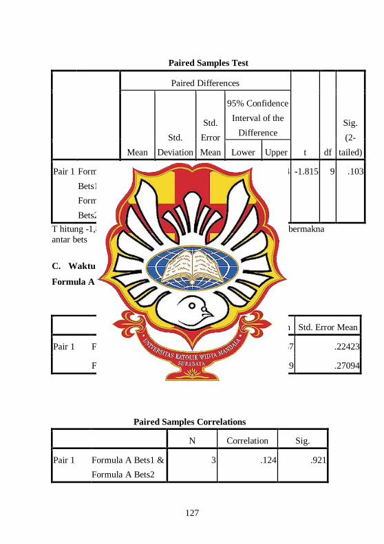
-.96000 1.67279 .52898 -2.15664 .23664 -1.815 9 .103

T hitung -1,815< T0,05 (9) = 1,833 sehingga tidak ada perbedaan bermakna antar bets

C. Waktu Hancur

Formula A


Pair 1 Formula A Bets1 10.9133 3 .38837 .22423

Formula A Bets2 10.7133 3 .46929 .27094


Pair 1 Formula A Bets1 & Formula A Bets2

3 .124 .921

128


t df

Sig. (2-

tailed)

Mean Std.

Deviation

Std. Error Mean



Pair 1 Formula A Bets1 – Formula A Bets2

.20000 .57088 .32960 -1.21814 1.61814 .607 2 .606


antar bets

Formula B


Pair 1 Formula B Bets1 10.0767 3 .58705 .33894

Formula B Bets2 10.3333 3 .98083 .56628


Pair 1 Formula1Bets1 & Formula1Bets2

3 -.938 .226

129

T hitung -0,288 < T0,05 (9) = 1,833 sehingga tidak ada perbedaan bermakna

antar bets

Formula C


Pair 1 Formula C Bets1 9.0200 3 .40951 .23643

Formula C Bets2 9.9700 3 .43715 .25239


Pair 1 Formula C Bets1 & Formula C Bets2

3 -.768 .442


t df

Sig. (2-

tailed)

Mean Std.

Deviation

Std. Error Mean



Pair 1 Formula B Bets1 – Formula B Bets2

-.25667 1.54484 .89191 -4.09426 3.58093 -.288 2 .801

130


t df

Sig. (2-

tailed)

Mean Std.

Deviation

Std. Error Mean


Difference

Lower Upper

Pair 1 Formula C Bets1 – Formula C Bets2

-.95000 .79618 .45967 -2.92782 1.02782 -2.067 2 .175


antar bets

Formula D


Pair 1 Formula D Bets1 10.6600 3 .46861 .27055

Formula D Bets2 10.8800 3 .60233 .34775


Pair 1 Formula D Bets1 & Formula D Bets2

3 .704 .503

131


t df

Sig. (2-

tailed)

Mean Std.

Deviation

Std. Error Mean



Pair 1 Formula D Bets1 – Formula D Bets2

-.22000 .43035 .24846 -1.28905 .84905 -.885 2 .469


antar bets

D. Tampilan Visual

Formula A


Mean N Std. Deviation Std. Error Mean

Pair 1 Formula A bets1 96.3600 10 .30623 .09684

Formula A bets2 97.7200 10 .15492 .04899


Pair 1 Formula A bets1 & Formula A bets2

10 -.005 .990

132


t df

Sig. (2-

tailed)

Mean

Std. Deviat

ion

Std. Error Mean



Pair 1 Formula A bets1 – formula A bets2

-1.36000 .34383 .10873 -1.60596 -1.11404 -12.508 9 .000


antar bets

Formula B


Pair 1 Formula B bets1 93.6300 10 .16364 .05175

Formula B bets2 93.6200 10 .24404 .07717


Pair 1 Formula B bets1 & Formula B bets2

10 -.323 .363

133


T df

Sig. (2-

tailed)

Mean Std.

Deviation

Std. Error Mean


Difference

Lower Upper

Pair 1 Formula B bets1 – Formula B bets2

.01000 .33483 .10588 -.22952 .24952 .094 9 .927


antar bets

Formula C


Mean N Std. Deviation Std. Error

Mean

Pair 1 Formula C bets1 96.5300 10 .25841 .08172

Formula C bets2 96.9200 10 .32249 .10198


Pair 1 Formula C bets1 & Formula C bets2

10 .419 .229

134

Paired Samples Test

Paired Differences

t df

Sig. (2-

tailed)

Mean Std.

Deviation

Std. Error Mean


Difference

Lower Upper

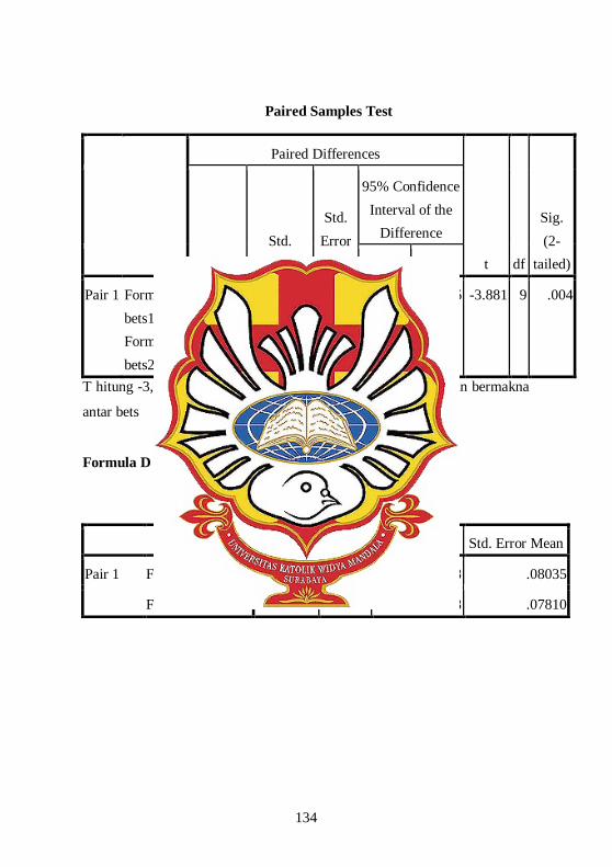
Pair 1 FormulaC bets1 – FormulaC bets2

-.39000 .31780 .10050 -.61734 -.16266 -3.881 9 .004


antar bets

Formula D


Pair 1 Formula D bets1 96.7700 10 .25408 .08035

Formula D bets2 97.1100 10 .24698 .07810

135


Pair 1 Formula D bets1 & Formula D bets2

10 .094 .797


t df

Sig. (2-

tailed)

Mean Std.

Deviation

Std. Error Mean



Pair 1 Formula D bets1 – Formula D bets2

-.34000 .33731 .10667 -.58130 -.09870 -3.187 9 .011


antar bets

136

LAMPIRAN G HASIL UJI STATISTIK ANTAR FORMULA TABLET SALUT

ENTERIK EKSTRAK TOMAT

A. Keseragaman Bobot

ANOVA

Keseragaman Bobot Sum of

Squares df Mean Square F Sig.

Between Groups 22.122 7 3.160 1.066 .388

Within Groups 450.747 152 2.965

Total 472.869 159

F hitung (1,066) < F0,05 = 2,07 tidak ada perbedaan bermakna antar formula

Post Hoc Tests


Keseragaman Bobot Tukey HSD

(I) Formula2

(J) Formula2

Mean Difference

(I-J) Std. Error Sig.


Lower Bound

Upper Bound

FA FB .80167 .54456 .821 -.8721 2.4754

FC .84167 .54456 .781 -.8321 2.5154

FD -.09833 .54456 1.000 -1.7721 1.5754

FA2 .05167 .54456 1.000 -1.6221 1.7254

FB2 -.02833 .54456 1.000 -1.7021 1.6454

137

FC2 -.07667 .54456 1.000 -1.7504 1.5971

FD2 -.03500 .54456 1.000 -1.7088 1.6388

FB FA -.80167 .54456 .821 -2.4754 .8721

FC .04000 .54456 1.000 -1.6338 1.7138

FD -.90000 .54456 .717 -2.5738 .7738

FA2 -.75000 .54456 .866 -2.4238 .9238

FB2 -.83000 .54456 .793 -2.5038 .8438

FC2 -.87833 .54456 .742 -2.5521 .7954

FD2 -.83667 .54456 .787 -2.5104 .8371

FC FA -.84167 .54456 .781 -2.5154 .8321

FB -.04000 .54456 1.000 -1.7138 1.6338

FD -.94000 .54456 .670 -2.6138 .7338

FA2 -.79000 .54456 .832 -2.4638 .8838

FB2 -.87000 .54456 .751 -2.5438 .8038

FC2 -.91833 .54456 .696 -2.5921 .7554

FD2 -.87667 .54456 .744 -2.5504 .7971

FD FA .09833 .54456 1.000 -1.5754 1.7721

FB .90000 .54456 .717 -.7738 2.5738

FC .94000 .54456 .670 -.7338 2.6138

FA2 .15000 .54456 1.000 -1.5238 1.8238

FB2 .07000 .54456 1.000 -1.6038 1.7438

FC2 .02167 .54456 1.000 -1.6521 1.6954

FD2 .06333 .54456 1.000 -1.6104 1.7371

138

FA2 FA -.05167 .54456 1.000 -1.7254 1.6221

FB .75000 .54456 .866 -.9238 2.4238

FC .79000 .54456 .832 -.8838 2.4638

FD -.15000 .54456 1.000 -1.8238 1.5238

FB2 -.08000 .54456 1.000 -1.7538 1.5938

FC2 -.12833 .54456 1.000 -1.8021 1.5454

FD2 -.08667 .54456 1.000 -1.7604 1.5871

FB2 FA .02833 .54456 1.000 -1.6454 1.7021

FB .83000 .54456 .793 -.8438 2.5038

FC .87000 .54456 .751 -.8038 2.5438

FD -.07000 .54456 1.000 -1.7438 1.6038

FA2 .08000 .54456 1.000 -1.5938 1.7538

FC2 -.04833 .54456 1.000 -1.7221 1.6254

FD2 -.00667 .54456 1.000 -1.6804 1.6671

FC2 FA .07667 .54456 1.000 -1.5971 1.7504

FB .87833 .54456 .742 -.7954 2.5521

FC .91833 .54456 .696 -.7554 2.5921

FD -.02167 .54456 1.000 -1.6954 1.6521

FA2 .12833 .54456 1.000 -1.5454 1.8021

FB2 .04833 .54456 1.000 -1.6254 1.7221

FD2 .04167 .54456 1.000 -1.6321 1.7154

FD2 FA .03500 .54456 1.000 -1.6388 1.7088

FB .83667 .54456 .787 -.8371 2.5104

139

FC .87667 .54456 .744 -.7971 2.5504

FD -.06333 .54456 1.000 -1.7371 1.6104

FA2 .08667 .54456 1.000 -1.5871 1.7604

FB2 .00667 .54456 1.000 -1.6671 1.6804

FC2 -.04167 .54456 1.000 -1.7154 1.6321 Homogeneous Subsets

Formula1

Tukey HSDa

Formula2 N


1

FC 20 415.9200

FB 20 415.9600

FA2 20 416.7100

FA 20 416.7617

FB2 20 416.7900

FD2 20 416.7967

FC2 20 416.8383

FD 20 416.8600

Sig. .670



140

B. Kekerasan

ANOVA

Kekerasan

Sum of Squares df Mean Square F Sig.

Between Groups

28.145 7 4.021 3.193 .005

Within Groups 90.670 72 1.259

Total 118.816 79

F hitung (3,193) > F0,05 = 2,014 ada perbedaan bermakna antar formula Post Hoc Tests


Kekerasan Tukey HSD

(I) formula2

(J) formula2

Mean Difference



Lower Bound

Upper Bound

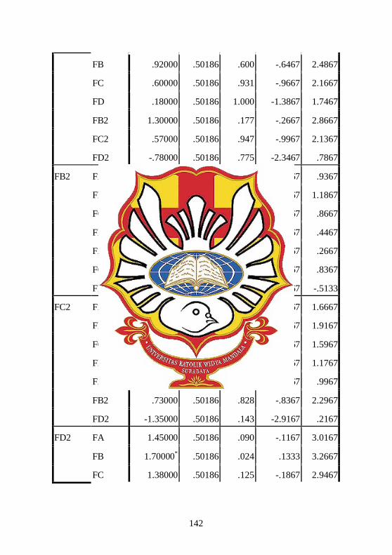
FA FB .25000 .50186 1.000 -1.3167 1.8167

FC -.07000 .50186 1.000 -1.6367 1.4967

FD -.49000 .50186 .976 -2.0567 1.0767

FA2 -.67000 .50186 .882 -2.2367 .8967

FB2 .63000 .50186 .912 -.9367 2.1967

FC2 -.10000 .50186 1.000 -1.6667 1.4667

141

FD2 -1.45000 .50186 .090 -3.0167 .1167

FB FA -.25000 .50186 1.000 -1.8167 1.3167

FC -.32000 .50186 .998 -1.8867 1.2467

FD -.74000 .50186 .818 -2.3067 .8267

FA2 -.92000 .50186 .600 -2.4867 .6467

FB2 .38000 .50186 .995 -1.1867 1.9467

FC2 -.35000 .50186 .997 -1.9167 1.2167

FD2 -1.70000* .50186 .024 -3.2667 -.1333

FC FA .07000 .50186 1.000 -1.4967 1.6367

FB .32000 .50186 .998 -1.2467 1.8867

FD -.42000 .50186 .990 -1.9867 1.1467

FA2 -.60000 .50186 .931 -2.1667 .9667

FB2 .70000 .50186 .857 -.8667 2.2667

FC2 -.03000 .50186 1.000 -1.5967 1.5367

FD2 -1.38000 .50186 .125 -2.9467 .1867

FD FA .49000 .50186 .976 -1.0767 2.0567

FB .74000 .50186 .818 -.8267 2.3067

FC .42000 .50186 .990 -1.1467 1.9867

FA2 -.18000 .50186 1.000 -1.7467 1.3867

FB2 1.12000 .50186 .346 -.4467 2.6867

FC2 .39000 .50186 .994 -1.1767 1.9567

FD2 -.96000 .50186 .547 -2.5267 .6067

FA2 FA .67000 .50186 .882 -.8967 2.2367

142

FB .92000 .50186 .600 -.6467 2.4867

FC .60000 .50186 .931 -.9667 2.1667

FD .18000 .50186 1.000 -1.3867 1.7467

FB2 1.30000 .50186 .177 -.2667 2.8667

FC2 .57000 .50186 .947 -.9967 2.1367

FD2 -.78000 .50186 .775 -2.3467 .7867

FB2 FA -.63000 .50186 .912 -2.1967 .9367

FB -.38000 .50186 .995 -1.9467 1.1867

FC -.70000 .50186 .857 -2.2667 .8667

FD -1.12000 .50186 .346 -2.6867 .4467

FA2 -1.30000 .50186 .177 -2.8667 .2667

FC2 -.73000 .50186 .828 -2.2967 .8367

FD2 -2.08000* .50186 .002 -3.6467 -.5133

FC2 FA .10000 .50186 1.000 -1.4667 1.6667

FB .35000 .50186 .997 -1.2167 1.9167

FC .03000 .50186 1.000 -1.5367 1.5967

FD -.39000 .50186 .994 -1.9567 1.1767

FA2 -.57000 .50186 .947 -2.1367 .9967

FB2 .73000 .50186 .828 -.8367 2.2967

FD2 -1.35000 .50186 .143 -2.9167 .2167

FD2 FA 1.45000 .50186 .090 -.1167 3.0167

FB 1.70000* .50186 .024 .1333 3.2667

FC 1.38000 .50186 .125 -.1867 2.9467

143

FD .96000 .50186 .547 -.6067 2.5267

FA2 .78000 .50186 .775 -.7867 2.3467

FB2 2.08000* .50186 .002 .5133 3.6467

FC2 1.35000 .50186 .143 -.2167 2.9167

*. The mean difference is significant at the 0.05 level. Homogeneous Subsets

Kekerasan

Tukey HSDa

formula2 N


1 2

FB2 10 6.5400

FB 10 6.9200

FA 10 7.1700 7.1700

FC 10 7.2400 7.2400

FC2 10 7.2700 7.2700

FD 10 7.6600 7.6600

FA2 10 7.8400 7.8400

FD2 10 8.6200

Sig. .177 .090



144

C. Waktu Hancur

ANOVA

Waktu Hancur Sum of


Between Groups

8.424 7 1.203 3.676 .015


Total 13.661 23

F hitung (3,676) < F0,05 = 2,66 tidak ada perbedaan bermakna antar

formula Post Hoc Tests


Waktu Hancur Tukey HSD

(I) formula2

(J) formula2

Mean Difference

(I-J) Std.

Error Sig.


Lower Bound

Upper Bound

FA FB .83667 .46717 .634 -.7807 2.4541

FC 1.89333* .46717 .016 .2759 3.5107

FD .25333 .46717 .999 -1.3641 1.8707

FA2 .20000 .46717 1.000 -1.4174 1.8174

FB2 .58000 .46717 .907 -1.0374 2.1974

145

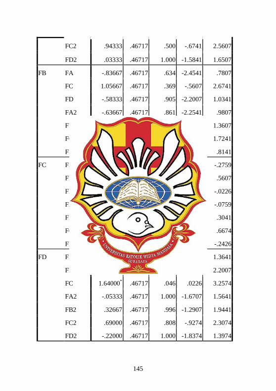
FC2 .94333 .46717 .500 -.6741 2.5607

FD2 .03333 .46717 1.000 -1.5841 1.6507

FB FA -.83667 .46717 .634 -2.4541 .7807

FC 1.05667 .46717 .369 -.5607 2.6741

FD -.58333 .46717 .905 -2.2007 1.0341

FA2 -.63667 .46717 .861 -2.2541 .9807

FB2 -.25667 .46717 .999 -1.8741 1.3607

FC2 .10667 .46717 1.000 -1.5107 1.7241

FD2 -.80333 .46717 .676 -2.4207 .8141

FC FA -1.89333* .46717 .016 -3.5107 -.2759

FB -1.05667 .46717 .369 -2.6741 .5607

FD -1.64000* .46717 .046 -3.2574 -.0226

FA2 -1.69333* .46717 .037 -3.3107 -.0759

FB2 -1.31333 .46717 .160 -2.9307 .3041

FC2 -.95000 .46717 .491 -2.5674 .6674

FD2 -1.86000* .46717 .019 -3.4774 -.2426

FD FA -.25333 .46717 .999 -1.8707 1.3641

FB .58333 .46717 .905 -1.0341 2.2007

FC 1.64000* .46717 .046 .0226 3.2574

FA2 -.05333 .46717 1.000 -1.6707 1.5641

FB2 .32667 .46717 .996 -1.2907 1.9441

FC2 .69000 .46717 .808 -.9274 2.3074

FD2 -.22000 .46717 1.000 -1.8374 1.3974

146

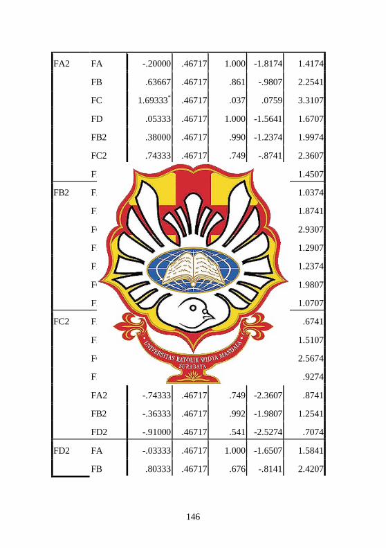
FA2 FA -.20000 .46717 1.000 -1.8174 1.4174

FB .63667 .46717 .861 -.9807 2.2541

FC 1.69333* .46717 .037 .0759 3.3107

FD .05333 .46717 1.000 -1.5641 1.6707

FB2 .38000 .46717 .990 -1.2374 1.9974

FC2 .74333 .46717 .749 -.8741 2.3607

FD2 -.16667 .46717 1.000 -1.7841 1.4507

FB2 FA -.58000 .46717 .907 -2.1974 1.0374

FB .25667 .46717 .999 -1.3607 1.8741

FC 1.31333 .46717 .160 -.3041 2.9307

FD -.32667 .46717 .996 -1.9441 1.2907

FA2 -.38000 .46717 .990 -1.9974 1.2374

FC2 .36333 .46717 .992 -1.2541 1.9807

FD2 -.54667 .46717 .929 -2.1641 1.0707

FC2 FA -.94333 .46717 .500 -2.5607 .6741

FB -.10667 .46717 1.000 -1.7241 1.5107

FC .95000 .46717 .491 -.6674 2.5674

FD -.69000 .46717 .808 -2.3074 .9274

FA2 -.74333 .46717 .749 -2.3607 .8741

FB2 -.36333 .46717 .992 -1.9807 1.2541

FD2 -.91000 .46717 .541 -2.5274 .7074

FD2 FA -.03333 .46717 1.000 -1.6507 1.5841

FB .80333 .46717 .676 -.8141 2.4207

147

FC 1.86000* .46717 .019 .2426 3.4774

FD .22000 .46717 1.000 -1.3974 1.8374

FA2 .16667 .46717 1.000 -1.4507 1.7841

FB2 .54667 .46717 .929 -1.0707 2.1641

FC2 .91000 .46717 .541 -.7074 2.5274

*. The mean difference is significant at the 0.05 level. Homogeneous Subsets

Waktu Hancur

Tukey HSDa

formula2 N


1 2

FC 3 9.0200

FC2 3 9.9700 9.9700

FB 3 10.0767 10.0767

FB2 3 10.3333 10.3333

FD 3 10.6600

FA2 3 10.7133

FD2 3 10.8800

FA 3 10.9133

Sig. .160 .500



148

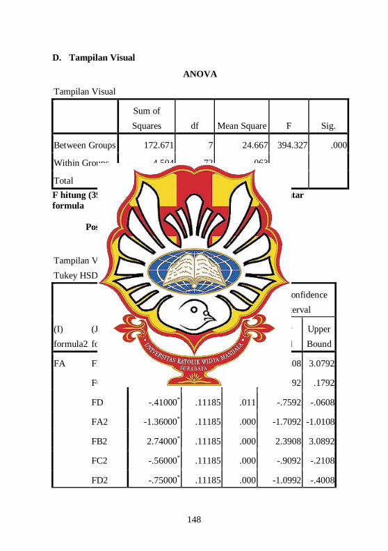
D. Tampilan Visual

ANOVA

Tampilan Visual Sum of


Between Groups 172.671 7 24.667 394.327 .000


Total 177.175 79

F hitung (394,327) > F0,05 = 2,14 ada perbedaan bermakna antar formula

Post Hoc Tests


Tampilan Visual Tukey HSD

(I) formula2

(J) formula2

Mean Difference



Lower Bound

Upper Bound

FA FB 2.73000* .11185 .000 2.3808 3.0792

FC -.17000 .11185 .794 -.5192 .1792

FD -.41000* .11185 .011 -.7592 -.0608

FA2 -1.36000* .11185 .000 -1.7092 -1.0108

FB2 2.74000* .11185 .000 2.3908 3.0892

FC2 -.56000* .11185 .000 -.9092 -.2108

FD2 -.75000* .11185 .000 -1.0992 -.4008

149

FB FA -2.73000* .11185 .000 -3.0792 -2.3808

FC -2.90000* .11185 .000 -3.2492 -2.5508

FD -3.14000* .11185 .000 -3.4892 -2.7908

FA2 -4.09000* .11185 .000 -4.4392 -3.7408

FB2 .01000 .11185 1.000 -.3392 .3592

FC2 -3.29000* .11185 .000 -3.6392 -2.9408

FD2 -3.48000* .11185 .000 -3.8292 -3.1308

FC FA .17000 .11185 .794 -.1792 .5192

FB 2.90000* .11185 .000 2.5508 3.2492

FD -.24000 .11185 .397 -.5892 .1092

FA2 -1.19000* .11185 .000 -1.5392 -.8408

FB2 2.91000* .11185 .000 2.5608 3.2592

FC2 -.39000* .11185 .018 -.7392 -.0408

FD2 -.58000* .11185 .000 -.9292 -.2308

FD FA .41000* .11185 .011 .0608 .7592

FB 3.14000* .11185 .000 2.7908 3.4892

FC .24000 .11185 .397 -.1092 .5892

FA2 -.95000* .11185 .000 -1.2992 -.6008

FB2 3.15000* .11185 .000 2.8008 3.4992

FC2 -.15000 .11185 .880 -.4992 .1992

FD2 -.34000 .11185 .062 -.6892 .0092

FA2 FA 1.36000* .11185 .000 1.0108 1.7092

FB 4.09000* .11185 .000 3.7408 4.4392

FC 1.19000* .11185 .000 .8408 1.5392

150

FD .95000* .11185 .000 .6008 1.2992

FB2 4.10000* .11185 .000 3.7508 4.4492

FC2 .80000* .11185 .000 .4508 1.1492

FD2 .61000* .11185 .000 .2608 .9592

FB2 FA -2.74000* .11185 .000 -3.0892 -2.3908

FB -.01000 .11185 1.000 -.3592 .3392

FC -2.91000* .11185 .000 -3.2592 -2.5608

FD -3.15000* .11185 .000 -3.4992 -2.8008

FA2 -4.10000* .11185 .000 -4.4492 -3.7508

FC2 -3.30000* .11185 .000 -3.6492 -2.9508

FD2 -3.49000* .11185 .000 -3.8392 -3.1408

FC2 FA .56000* .11185 .000 .2108 .9092

FB 3.29000* .11185 .000 2.9408 3.6392

FC .39000* .11185 .018 .0408 .7392

FD .15000 .11185 .880 -.1992 .4992

FA2 -.80000* .11185 .000 -1.1492 -.4508

FB2 3.30000* .11185 .000 2.9508 3.6492

FD2 -.19000 .11185 .688 -.5392 .1592

FD2 FA .75000* .11185 .000 .4008 1.0992

FB 3.48000* .11185 .000 3.1308 3.8292

FC .58000* .11185 .000 .2308 .9292

FD .34000 .11185 .062 -.0092 .6892

FA2 -.61000* .11185 .000 -.9592 -.2608

151

FB2 3.49000* .11185 .000 3.1408 3.8392

FC2 .19000 .11185 .688 -.1592 .5392

*. The mean difference is significant at the 0.05 level.

Homogeneous Subsets

Tampilan Visual

Tukey HSDa

formula2 N


1 2 3 4 5

FB2 10 93.6200

FB 10 93.6300

FA 10 96.3600

FC 10 96.5300 96.5300

FD 10 96.7700 96.7700

FC2 10 96.9200

FD2 10 97.1100

FA2 10 97.7200

Sig. 1.000 .794 .397 .062 1.000



152

LAMPIRAN H

HASIL UJI MUTU FISIK LARUTAN PENYALUT TABLET SALUT ENTERIK EKSTRAK TOMAT

A. UJI BERAT JENIS

Tabel 4.33. Hasil uji berat jenis larutan penyalut

Formula

Replikasi

Berat piknometer Berat zat (g)

Vol. piknometer

ρ (m/v)

X ± SD Berat kosong (g)

Berat kosong + zat (g)

A 1 22,2028 44,7099 22,5071 25,00 1,0137 1,0185 ± 0,0092 2 22,2222 44,7286 22,5064 25,00 1,0128

3 22,0372 44,7155 22,6783 25,00 1,0291 B 1 22,2128 45,2103 22,9975 25,00 1,0353 1,0395 ±

0,0043 2 22,1827 45,3410 23,1583 25,00 1,0440 3 22,2078 45,2857 23,0779 25,00 1,0392 C 1 22,2415 44,7255 22,4840 25,00 1,0109 1,0134 ±

0,0024 2 22,2310 44,8110 22,5800 25,00 1,0157 3 22,2265 44,7554 22,5289 25,00 1,0136 D 1 22,2197 44,5147 22,2950 25,00 1,0214 1,0213 ±

0,0005 2 22,2210 44,9259 22,7049 25,00 1,0218 3 22,2187 44,8975 22,6788 25,00 1,0207

153

B. UJI VISKOSITAS

Tabel 4.34. Hasil uji viskositas larutan penyalut

Formula Replikasi No. Spindle

Laju Putar (Rpm)

Angka terbaca

X ± SD

A 1 1 100 25,0 24,37 ± 0,55 2 1 100 24,0

3 1 100 24,1 B 1 1 30 138,2

139 ± 0,8 2 1 30 139,0 3 1 30 139,8

C 1 1 100 22,4 22,57 ± 0,15 2 1 100 22,7

3 1 100 22,6 D 1 1 30 102,0

102,6 ± 0,72 2 1 30 103,4 3 1 30 102,4

154

LAMPIRAN I

HASIL ANALISIS DATA DENGAN DESIGN EXPERT SECARA FAKTOR DESIGN UNTUK RESPON KEKERASAN TABLET

SALUT ENTERIK EKSTRAK TOMAT Response 1 Kekerasan (kgf) ANOVA for selected factorial model Analysis of variance table [Partial sum of squares - Type III] Sum of Mean F p-value Source Squares df Square Value Prob > F Model 2.38 3 0.79 7.06 0.0448 significant A-HPMCP 1.57 1 1.57 13.93 0.0202 B-PEG 6000 0.045 1 0.045 0.40 0.5613 AB0.77 1 0.77 6.84 0.0591 Pure Error 0.45 4 0.11 Cor Total 2.83 7 The Model F-value of 7.06 implies the model is significant. There is only a 4.48% chance that a "Model F-Value" this large could occur due to noise. Values of "Prob > F" less than 0.0500 indicate model terms are significant. In this case A are significant model terms. Values greater than 0.1000 indicate the model terms are not significant. If there are many insignificant model terms (not counting those required to support hierarchy), model reduction may improve your model. Std. Dev. 0.34 R-Squared 0.8411 Mean 7.40 Adj R-Squared 0.7219 C.V. % 4.53 Pred R-Squared 0.3644 PRESS 1.80 Adeq Precision 6.348 The "Pred R-Squared" of 0.3644 is not as close to the "Adj R-Squared" of 0.7219 as one might normally expect. This may indicate a large block effect or a possible problem with your model and/or data. Things to consider are model reduction, response transformation, outliers, etc.

155

"Adeq Precision" measures the signal to noise ratio. A ratio greater than 4 is desirable. Your ratio of 6.348 indicates an adequate signal. This model can be used to navigate the design space. Coefficient Standard 95% CI 95% CI Factor Estimate df Error Low High VIF Intercept 7.40 1 0.12 7.07 7.73 A-HPMCP -0.44 1 0.12 -0.77 -0.11 1.00 B-PEG 6000 0.075 1 0.12 -0.25 0.40 1.00 AB-0.31 1 0.12 -0.64 0.019 1.00 Final Equation in Terms of Coded Factors: Kekerasan (kgf) = +7.40 -0.44 * A +0.075 * B -0.31 * A * B Final Equation in Terms of Actual Factors: Kekerasan (kgf) = +7.39750 -0.44250 * HPMCP +0.075000 * PEG 6000 -0.31000 * HPMCP * PEG 6000 The Diagnostics Case Statistics Report has been moved to the Diagnostics Node. In the Diagnostics Node, Select Case Statistics from the View Menu. Proceed to Diagnostic Plots (the next icon in progression). Be sure to look at the:

156

1) Normal probability plot of the studentized residuals to check for normality of residuals. 2) Studentized residuals versus predicted values to check for constant error. 3) Externally Studentized Residuals to look for outliers, i.e., influential values. 4) Box-Cox plot for power transformations. If all the model statistics and diagnostic plots are OK, finish up with the Model Graphs icon.

157

LAMPIRAN J HASIL ANALISIS DATA DENGAN DESIGN EXPERT SECARA

FAKTOR DESIGN UNTUK RESPON WAKTU HANCUR TABLET SALUT ENTERIK EKSTRAK TOMAT

Response 2 Waktu hancur (menit) ANOVA for selected factorial model Analysis of variance table [Partial sum of squares - Type III] Sum of Mean F p-value Source Squares df Square Value Prob > F Model 1.60 3 0.53 11.44 0.0197 significant A-HPMCP 0.86 1 0.86 18.46 0.0127 B-PEG 6000 0.73 1 0.73 15.75 0.0166 AB5.000E-003 1 5.000E-003 0.11 0.7594 Pure Error 0.19 4 0.046 Cor Total 1.78 7 The Model F-value of 11.44 implies the model is significant. There is only a 1.97% chance that a "Model F-Value" this large could occur due to noise. Values of "Prob > F" less than 0.0500 indicate model terms are significant. In this case A, B are significant model terms. Values greater than 0.1000 indicate the model terms are not significant. If there are many insignificant model terms (not counting those required to support hierarchy), model reduction may improve your model. Std. Dev. 0.22 R-Squared 0.8956 Mean 10.20 Adj R-Squared 0.8173 C.V. % 2.11 Pred R-Squared 0.5825 PRESS 0.74 Adeq Precision 8.266 The "Pred R-Squared" of 0.5825 is not as close to the "Adj R-Squared" of 0.8173 as one might normally expect. This may indicate a large block effect or a possible problem with your model and/or data. Things to consider are model reduction, response

158

transformation, outliers, etc. "Adeq Precision" measures the signal to noise ratio. A ratio greater than 4 is desirable. Your ratio of 8.266 indicates an adequate signal. This model can be used to navigate the design space. Coefficient Standard 95% CI 95% CI Factor Estimate df Error Low High VIF Intercept 10.21 1 0.076 9.99 10.42 A-HPMCP 0.33 1 0.076 0.12 0.54 1.00 B-PEG 6000 0.30 1 0.076 0.091 0.51 1.00 AB-0.025 1 0.076 -0.24 0.19 1.00 Final Equation in Terms of Coded Factors: Waktu hancur (menit) = +10.21 +0.33 * A +0.30 * B -0.025 * A * B Final Equation in Terms of Actual Factors: Waktu hancur (menit) = +10.20500 +0.32750 * HPMCP +0.30250 * PEG 6000 -0.025000 * HPMCP * PEG 6000 The Diagnostics Case Statistics Report has been moved to the Diagnostics Node. In the Diagnostics Node, Select Case Statistics from the View Menu. Proceed to Diagnostic Plots (the next icon in progression). Be sure to look at the:

159

1) Normal probability plot of the studentized residuals to check for normality of residuals. 2) Studentized residuals versus predicted values to check for constant error. 3) Externally Studentized Residuals to look for outliers, i.e., influential values. 4) Box-Cox plot for power transformations. If all the model statistics and diagnostic plots are OK, finish up with the Model Graphs icon.

160

LAMPIRAN K HASIL ANALISIS DATA DENGAN DESIGN EXPERT SECARA

FAKTOR DESIGN UNTUK RESPON TAMPILAN VISUAL TABLET SALUT ENTERIK EKSTRAK TOMAT

Response 3 Tampilan Visual (%) ANOVA for selected factorial model Analysis of variance table [Partial sum of squares - Type III] Sum of Mean F p-value Source Squares df Square Value Prob > F Model 16.49 3 5.50 28.32 0.0037 significant A-HPMCP 3.35 1 3.35 17.28 0.0142 B-PEG 6000 7.22 1 7.22 37.20 0.0037 AB5.92 1 5.92 30.49 0.0053 Pure Error 0.78 4 0.19 Cor Total 17.27 7 The Model F-value of 28.32 implies the model is significant. There is only a 0.37% chance that a "Model F-Value" this large could occur due to noise. Values of "Prob > F" less than 0.0500 indicate model terms are significant. In this case A, B, AB are significant model terms. Values greater than 0.1000 indicate the model terms are not significant. If there are many insignificant model terms (not counting those required to support hierarchy), model reduction may improve your model. Std. Dev. 0.44 R-Squared 0.9550 Mean 96.08 Adj R-Squared 0.9213 C.V. % 0.46 Pred R-Squared 0.8202 PRESS 3.11 Adeq Precision 11.621 The "Pred R-Squared" of 0.8202 is in reasonable agreement with the "Adj R-Squared" of 0.9213. "Adeq Precision" measures the signal to noise ratio. A ratio greater than 4 is desirable. Your

161

ratio of 11.621 indicates an adequate signal. This model can be used to navigate the design space. Coefficient Standard 95% CI 95% CI Factor Estimate df Error Low High VIF Intercept 96.08 1 0.16 95.65 96.51 A-HPMCP -0.65 1 0.16 -1.08 -0.22 1.00 B-PEG 6000 0.95 1 0.16 0.52 1.38 1.00 AB0.86 1 0.16 0.43 1.29 1.00 Final Equation in Terms of Coded Factors: Tampilan Visual (%) = +96.08 -0.65 * A +0.95 * B +0.86 * A * B Final Equation in Terms of Actual Factors: Tampilan Visual (%) = +96.08250 -0.64750 * HPMCP +0.95000 * PEG 6000 +0.86000 * HPMCP * PEG 6000 The Diagnostics Case Statistics Report has been moved to the Diagnostics Node. In the Diagnostics Node, Select Case Statistics from the View Menu. Proceed to Diagnostic Plots (the next icon in progression). Be sure to look at the: 1) Normal probability plot of the studentized residuals to check for normality of residuals. 2) Studentized residuals versus predicted values to check for constant error. 3) Externally Studentized Residuals to look for outliers, i.e., influential values.

162

4) Box-Cox plot for power transformations. If all the model statistics and diagnostic plots are OK, finish up with the Model Graphs icon.

163

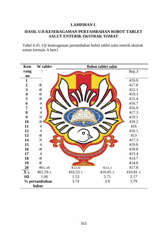
LAMPIRAN L

HASIL UJI KESERAGAMAN PERTAMBAHAN BOBOT TABLET SALUT ENTERIK EKSTRAK TOMAT

Tabel 4.35. Uji keseragaman pertambahan bobot tablet salut enterik ekstrak tomat formula A bets1

Keterangan

W tablet inti

Bobot tablet salut Rep. 1 Rep.2 Rep.3

1 403 414 419.1 419.9 2 404.23 415.5 417.9 417.8 3 401.16 416.8 419.2 412.1 4 400.53 419 418.3 419.3 5 401.43 417 418.5 415.4 6 403.8 416.7 415.9 416.7 7 403.6 415.8 410.3 416.9 8 400.3 418.5 419.2 417.3 9 398.23 419.1 416.4 419.1 10 400.03 415.9 419.1 418.2 11 401.9 418.8 414.9 416 12 402.4 417 419 416.1 13 402.46 416.1 416 413 14 398.63 414.6 417 417.3 15 401.1 416.7 407.2 419.8 16 401.36 417.4 435.2 418.8 17 401.9 414.6 415.8 415.4 18 403.93 418.2 417.8 414.7 19 400.26 415.2 407.1 414.6 20 401.56 415.6 413.1 417.8

X ± SD

401.59 ± 1.66

416.53 ± 1.53

416.85 ± 5.71

416.81 ± 2.17

% pertambahan bobot

3.74 3.8 3.79

164

Tabel 4.36. Uji keseragaman pertambahan bobot tablet salut enterik ekstrak tomat formula B bets1

Keterangan

W tablet inti


1 397.3 416.2 411.8 410.7 2 404.93 418.1 418.5 416.9 3 400.5 416.7 411.8 417.3 4 403.8 412.8 417.4 416.6 5 398.76 414.4 415.6 416.7 6 398.33 414.7 418 410.5 7 401.4 414.4 416.6 416.3 8 398.46 416.7 412.8 414.9 9 395.66 410 411.3 415.6 10 398.5 417.3 416.9 414.5 11 396.13 416.1 416.8 415.8 12 401.23 416.4 418 417.2 13 400.96 417.4 416.2 417.6 14 402.26 416.9 417.8 417.1 15 401.53 416 415.7 417.1 16 400.8 417.8 417.3 418 17 401.3 417.3 418.5 416.3 18 400.7 416.4 416.6 416.7 19 399.56 417.4 415.9 416 20 400.06 416.1 415.98 417.1

X ± SD

400.11 ± 2.33

416 ± 1.92

416.38 ± 2.26

415.95 ± 2.02

% pertambahan bobot

3.97 3.96 3.96

165

Tabel 4.37. Uji keseragaman pertambahan bobot tablet salut enterik ekstrak tomat formula C bets1

Keteranga

n

W tablet inti


1 398.9 415.2 412 418.1 2 403.46 414.7 417.9 416.9 3 400.03 412.1 416.1 417.9 4 398.93 416.9 415.6 407 5 400.63 416 416.6 417.8 6 399.76 417.8 413.1 416.2 7 398.9 416.6 416.9 417.1 8 403 417.7 412.8 413.5 9 397.96 417.5 417.8 417.6

10 399.13 418.2 416.3 418.9 11 401.96 416.1 415 411 12 400.76 416.6 416.8 412.5 13 399.26 417.4 415.9 416.5 14 402.66 416.6 413.5 410.8 15 401.86 416.8 418.7 415.8 16 403.23 416.8 415 420.5 17 401.3 415.8 415.1 416.7 18 400.33 411.2 418.4 418 19 398.63 417.3 416.7 418.3 20 397.6 411.9 417.4 417.3

X ± SD

400.42 ± 1.8

415.96 ± 2.02

415.88 ± 1.89

415.92 ± 3.30

% pertambahan bobot

3.88 3.86 3.87

166

Tabel 4.38. Uji keseragaman pertambahan bobot tablet salut enterik ekstrak tomat formula D bets1

Keteranga

n

W tablet inti


1 402.06 417.5 418.4 418.5 2 401.9 417.9 418.5 415.7 3 400.83 416 417.3 418.1 4 403.26 412.4 416.9 419.5 5 403.03 417.3 419.7 418.4 6 397.93 410.1 416 416.3 7 398.26 418.9 417.1 416.2 8 400.1 419.2 418.8 418.1 9 401 416.8 417.8 419 10 400.86 418.2 415.7 411.5 11 399.73 419.5 412.2 418.9 12 398.13 418.9 410.1 410.2 13 402.63 415.9 415.8 418.7 14 402.26 416.5 416.7 416.9 15 402.66 419.2 419.5 419.7 16 401.5 416.1 416.9 410.3 17 401.06 412.4 418.5 418.8 18 401.2 417.5 416.5 416.6 19 400.96 418.8 415.7 418.3 20 401.23 416.3 419.4 419

X ± SD

401.03 ± 1.56

416.77 ± 2.53

416.87 ± 2.36

416.9 ± 2.94

% pertambahan bobot

3.92 3.95 3.96

167

Tabel 4.39. Uji keseragaman pertambahan bobot tablet salut enterik ekstrak tomat formula A bets2

Keteranga

n

W tablet inti


1 402.16 418.8 414.9 416 2 398.66 417 419 416.1 3 403.53 416.1 416 413 4 401.63 414.6 417 417.3 5 401.7 416.7 407.2 419.8 6 401.7 417.4 435.2 418.8 7 402.53 414.6 415.8 415.4 8 402.43 418.2 417.8 414.7 9 401.8 415.2 407.1 414.6 10 399.83 415.6 413.1 417.8 11 403.36 418.5 418.4 417.5 12 402.4 415.7 418.5 417.9 13 400.03 418.1 417.3 416 14 400.3 419.5 416.9 412.4 15 399.6 418.4 419.7 417.3 16 400.1 416.3 416 410.1 17 398.83 416.2 417.1 418.9 18 401.86 418.1 418.8 419.2 19 400.43 419 417.8 416.8 20 399.2 411.5 415.7 418.2

X ± SD

401.11 ± 1.48

416.78 ± 1.94

416.96 ± 5.48

416.4 ± 2.48

% pertambahan bobot

3.90 3.95 3.81

168

Tabel 4.40. Uji keseragaman pertambahan bobot tablet salut enterik ekstrak tomat formula B bets2

Keterangan

W tablet inti


1 402.73 416.1 416.8 418.8 2 402.23 419.4 418 417.2 3 401.43 417.4 416.2 417.6 4 400.26 416.9 417.8 417.1 5 401.76 416 418.7 417.1 6 402.16 417.8 417.3 418 7 401.06 417.3 418.5 418.3 8 401.33 416.4 416.6 416.7 9 401.2 417.4 418.9 416 10 402.16 416.1 416.1 417.1 11 402.33 418.1 412 415.2 12 401.13 416.9 417.9 414.7 13 401.86 417.9 416.1 412.1 14 401.93 407 415.6 416.9 15 400.96 417.8 416.6 416 16 402.66 416.2 413.1 417.8 17 401.9 417.1 416.9 416.6 18 403.93 413.5 419.8 417.7 19 400.26 417.6 417.8 417.5 20 401.56 418.9 418.3 418.2

X ± SD

401.75 ± 0.86

416.6 ± 2.57

416.95 ± 1.87

416.83 ± 1.51

% pertambahan bobot

3.70 3.78 3.75

169

Tabel 4.41. Uji keseragaman pertambahan bobot tablet salut enterik ekstrak tomat formula C bets2

Keteranga

n

W tablet inti


1 403.36 415 411 419.5 2 401.56 416.8 412.5 418.9 3 404.2 415.9 419.5 415.9 4 403.36 413.5 410.8 416.5 5 401.66 418.7 419.8 419.2 6 404 415 420.5 416.1 7 399.53 415.1 416.7 412.4 8 401.66 418.4 418 417.5 9 400.76 416.7 418.3 418.8 10 403.53 417.4 417.3 416.3 11 401.46 418.8 419.1 414 12 401.03 418.5 417.9 415.5 13 400.5 419.8 419.2 416.8 14 399.16 417.4 418.3 419 15 402.23 415.6 418.5 417 16 402.73 418 415.9 416.7 17 401.4 416.6 410.3 415.8 18 403.03 415.8 419.2 418.5 19 401.1 417.3 416.4 419.1 20 400.7 418.9 419.1 415.9

X ± SD

401.85 ± 1.42

416.96 ± 1.65

416.9 ± 3.19

417 ± 1.87

% pertambahan bobot

3.76 3.74 3.77

170

Tabel 4.42. Uji keseragaman pertambahan bobot tablet salut enterik ekstrak tomat formula D bets2

Keteranga

n

W tablet inti


1 404.1 419.5 412.2 418.9 2 402.33 418.9 410.1 410.2 3 403.03 415.9 415.8 418.7 4 398.26 416.5 416.7 416.9 5 402.83 419.2 419.5 419.7 6 400.33 416.1 416.9 410.3 7 395.3 412.4 418.5 418.8 8 399.4 417.5 416.5 416.6 9 404.63 418.8 415.7 418.3

10 401.33 416.3 419.4 419 11 398.9 414 410.7 419.9 12 400.23 415.5 416.9 417.8 13 400.83 416.8 417.3 412.1 14 401.23 419 418.6 419.3 15 402.46 417 416.7 415.4 16 404.06 416.7 410.5 416.7 17 402.96 415.8 418.3 416.9 18 401.93 418.5 418.9 417.3 19 400.86 419.1 419.6 419.1 20 398.63 415.9 419.5 418.2

X ± SD

401.18 ± 2.31

417 ± 1.65

416.41 ± 3.11

417 ± 2.91

% pertambahan bobot

3.94 3.79 3.94

171

LAMPIRAN M

HASIL PERHITUNGAN KONVERSI NILAI TINGKAT MENJADI NILAI RIIL

Contoh hasil perhitungan konversi nilai tingkat menjadi nilai riil

X’ = X – rata-rata 2 level

½ x perbedaan level

X’ : level dalam bentuk baku

X : level sesungguhnya (level dalam bentuk %)

HPMCP : -1,00 = X – 7,5

½ x 5

X = 5 %

PEG 6000 : -1,00 = X – 0,75

½ x 0,5

X = 0,5 %

172

LAMPIRAN N

SERTIFIKAT ANALISIS PEMBELIAN EKSTRAK TOMAT

173

LAMPIRAN O

SERTIFIKAT ANALISIS PEMBELIAN BAHAN

CROSCARMELLOSE SODIUM

174

LAMPIRAN P

SERTIFIKAT ANALISIS PEMBELIAN BAHAN KALSIUM FOSFAT DIBASIK

175

LAMPIRAN Q

HASIL PENILAIAN TAMPILAN VISUAL PANELIS TABLET SALUT ENTERIK EKSTRAK TOMAT

A. Pemeriksaan Visual Panelis I

176

B. Pemeriksaan Visual Panelis II

177

C. Pemeriksaan Visual Panelis III

178

D. Pemeriksaan Visual Panelis VI

179

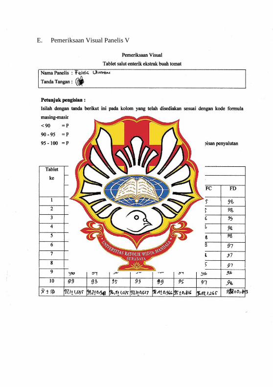
E. Pemeriksaan Visual Panelis V

180

F. Pemeriksaan Visual Panelis VI

181

G. Pemeriksaan Visual Panelis VII

182

H. Pemeriksaan Visual Panelis VIII

183

I. Pemeriksaan Visual Panelis IX

184

J. Pemeriksaan Visual Panelis X

185

LAMPIRAN R TABEL UJI F

186

TABEL F UJI (LANJUTAN)

187

TABEL F UJI (LANJUTAN)

188

LAMPIRAN S GAMBAR EKSTRAK TOMAT, TABLET INTI EKSTRAK TOMAT,

DAN TABLET SALUT ENTERIK EKSTRAK TOMAT

Ekstrak Tomat

Tablet Inti Ekstrak Tomat Tablet Salut Enterik Ekstrak Tomat

lampiran a hasil pengamatan standarisasi …repository.wima.ac.id/727/7/lampiran.pdf · hasil...

Documents