laminar flow control: back to the future? (invited)

American Institute of Aeronautics and Astronautics

092407

1

Laminar Flow Control – Back to the Future?

John E. Green1 Aircraft Research Association Ltd., Bedford UK, MK41 7PF

In the 21st Century, reducing the environmental impact of aviation will become an increasingly important

priority for the aircraft designer. Among the various environmental impacts, emission of CO2 can be expected

to emerge as the most important in the long term and reducing fuel burn to become the overriding

environmental priority. Increasing fuel costs and the world’s limited oil reserves will add to the pressure to

reduce fuel burn. Starting from the limitations imposed on the aircraft designer by the laws of physics – the

Breguet Range Equation, the Second Law of Thermodynamics, the behaviour of real, viscous fluids – the

paper discusses the technological and design options available to the designer. Improvements in propulsion

and structural efficiency have valuable contributions to make but it is in drag reduction through laminar flow

control that the greatest opportunity lies. The physics underlying laminar flow control is discussed and the

key features and limitations of natural, hybrid and full laminar flow control are explained. Experience to date

in this field is briefly reviewed, with particular attention drawn to the substantial body of work in the 1950s

and 1960s that demonstrated the potential of full laminar flow control by boundary-layer suction. The case is

argued for revisiting the design of an aircraft with full laminar flow control, taking into account the advances

over the past half century in all aspects of aircraft engineering, notably in propulsion and materials. With

approximately half the thrust provided by the boundary layer suction system, this aircraft presents a

completely new challenge in airframe-propulsion integration. We understand the physics of boundary layer

control, we know that an aircraft with full laminar flow is potentially much more fuel efficient than the

alternatives, what is needed now is a wholehearted attack on the engineering obstacles in its path.

Nomenclature

Symbols A = aspect ratio (= b2/S) a,b = constants in Lanchester’s drag formulation b = wing span CD = drag coefficient (= D/qS) CDO = drag coefficient at zero lift Cf = skin friction coefficient (= 2τW//ρU2) CL = lift coefficient (= L/qS) D = drag Di = induced drag F = Lanchester’s tangential force g = gravitational acceleration H = calorific value of fuel (energy per unit mass) H = boundary layer shape parameter (= δ*/θ) L = lift (L/D)M = maximum lift/drag ratio M = Mach number p = static pressure q = dynamic pressure ( = 0.7pM2) (q)M = value of q at (L/D)M R = range S = wing area SDO = drag area ( = D/q ) at zero lift ThS = specific thrust ( = net thrust per unit mass of engine air flow) u = streamwise velocity component within boundary layer U = streamwise velocity at edge of boundary layer v = velocity component normal to surface within boundary layer 1 Consultant Chief Scientist, 1 Leighton Street, Woburn, Milton Keynes, MK17 9PJ, UK, AIAA Fellow

38th Fluid Dynamics Conference and Exhibit<BR> 23 - 26 June 2008, Seattle, Washington

AIAA 2008-3738

Copyright © 2008 by John Green. Published by the American Institute of Aeronautics and Astronautics, Inc., with permission.


092407

2

vS = suction velocity (= - vW) vW = velocity at porous wall (positive away from surface) V = flight velocity V1 = flight velocity at maximum L/D V2 = flight velocity at minimum power W = aircraft weight in flight WE = aircraft empty weight WMF =.weight of mission fuel WP = weight of payload X = aircraft range parameter ( = HηL/D) x = streamwise distance in boundary layer y = distance normal to surface in boundary layer` δ

* = boundary layer displacement thickness η = overall propulsive efficiency ( = ηthermηtransηprop) ηtherm = engine thermal efficiency ηtrans = transfer efficiency ηprop = propulsive efficiency of jet (Froude efficiency) θ = boundary layer momentum thickness κ = vortex drag factor (unity for elliptically loaded wing) λ = q/(q)M µ = absolute viscosity ρ = density

I. Introduction

Laminar flow control has been with us for nearly 70 years. In March 1940 the British government placed an order on North American Aviation to design and build a new fighter aircraft for the Royal Air Force. The new aircraft was designated P-51 and incorporated a wing with a natural laminar flow aerofoil section developed by NACA. The laminar flow wing gave the P-51 outstanding speed and range and made it one of the most successful aircraft of World War II, particularly in the role of long-range bomber escort. In the following two decades there was a substantial amount of research into laminar flow control, much of it

into the use of boundary layer suction to achieve laminar flow. The research showed the feasibility of laminar flow control by suction and identified the practical problems to be overcome but did not lead to the manufacture of any large aircraft incorporating the technology. Although since the 1960s the level of interest in laminar flow has fluctuated with the price of oil, the price has never stayed high enough for long enough to persuade any aircraft manufacturer to take the plunge. It has been left to the sailplane designers to develop natural laminar flow aerofoils and this they have done with great success, so much so that it may require a further step, such as the introduction of boundary layer suction, to progress further. June 2008 is a fitting time to revisit the

possibilities for laminar flow control. Over the past decade, international concern about the impact of the growth in air travel on the world’s climate has been growing steadily. Reducing CO2 emissions from aircraft, which means reducing fuel burn, has become an environmental priority for the airlines and the manufacturing industry alike. In addition, since 2001, the price of oil has increased from $20 per barrel to values in the range $120 to $140 at the time of writing. Sustained oil prices at anything approaching these recent levels will augment substantially the priority given by operators and manufacturers to reducing fuel burn.

Figure 1. North American P-51 Mustang


092407

3

This paper briefly reviews the contribution of the emissions from aviation to climate change and concludes that reducing CO2 emissions – i.e. reducing fuel burn - is the most important long-term objective. It then reviews the laws of physics which set boundaries on what can be achieved in this respect and considers the options available to the designer and operator. It concludes that, while every option must be pursued, the technology with the greatest potential is the reduction of profile drag through laminar flow control. The underlying physics of laminar flow control is discussed for all three classes of control, natural, hybrid and full, and the steps needed to bring these to fruition are discussed. In particular, the paper calls for a re-assessment of the concept of the fully laminar aircraft, as set out by Handley Page in 1961, in the light of the advances in structures and propulsion over the past 47 years.

II. Environmental and Economic Drivers

A. Environment

There are three important ways in which air travel impacts the environment: noise in the neighbourhood of airports; air quality around airports; and contribution to climate change through emissions at altitude. There is a degree of conflict between these objectives – for example, measures to reduce noise can increase fuel burn and CO2 emissions while measures to improve fuel efficiency by increasing engine overall pressure ratio increase the emission of the oxides of nitrogen which adversely effect local air quality. Noise and local air quality are subject to ICAO regulations which we can expect to be tightened progressively as technology advances and further increases in stringency become affordable. They will not be discussed further. The third environmental impact, on the world’s climate, is now generally regarded as the most important. It comes about through the emission at altitude of gases and particles in the engine exhaust which, directly or indirectly, increase or reduce the greenhouse effect. The measure currently adopted for this impact is radiative forcing (RF), the perturbation caused by human activity to the energy balance between incoming solar radiation and outgoing infra-red radiation from the earth and the atmosphere. It is measured in W/m2; the estimate1 by the Intergovernmental Panel on Climate Change (IPCC) of RF in 2005 from all human activity since the beginning of the industrial revolution is approximately 1.6W/m2, arising from a positive contribution of approximately 3.0W/m2 from greenhouse gases offset by a negative contribution from soot and other aerosol emissions from human activity.

Table 1 shows the contributions and lifetimes of the five main anthropogenic greenhouse gases∗ together with the lifetimes at the tropopause of the oxides of nitrogen and of contrails and cirrus cloud, both of which play a part in aviation’s impact on climate. Nitrous oxide (N2O), a long lived greenhouse gas, is not a significant component of aircraft emissions. However, two other oxides of nitrogen, NO and NO2, collectively termed NOX, which are not themselves greenhouse gases but greenhouse gas precursors, are a significant component of aircraft emissions. They are relatively short lived but, when emitted at altitude, they alter the atmospheric concentrations of ozone and methane, increasing ozone and reducing methane, both strong greenhouse gases.

Table 1. Anthropogenic greenhouse gas concentrations, lifetimes and radiative forcing

Concentration, ppm Gas

Pre-1750 Current

Lifetime, years

Increased RF, W/m2-

Carbon dioxide (CO2) 280 380 50 - 200 1.66

Methane (CH4) 0.7 1.8 12 0.5

Tropospheric ozone (O3) 0.025 0.034 hours - days 0.35

Nitrous oxide (N2O) 0.27 0.32 114 0.16

Halocarbons 0 0.001 5 - 10,000 0.34

Precursors and other main contributors from aviation

NOX (NO and NO2) days

Contrails and cirrus cloud hours

∗ from http://cdiac.ornl.gov/pns/current_ghg.html, cited 12 June 2008


092407

4

The estimated radiative forcing from the three main contributors from aviation, CO2, NOX and contrails taken together with cirrus cloud, is given in Table 2. Since the contribution from aviation is only a small fraction of the anthropogenic total, the units in Table 2 are mW/m2.

Table 2. Main contributions to climate change from aviation

The great uncertainty in the estimated contribution of contrails and contrail cirrus derives mostly from uncertainly in the impact of cirrus cloud. The best estimate for the RF from contrails alone3, 10mW/m2, is itself subject to appreciable uncertainty (3 – 30mW/m2), as are the effects of NOX, the values in Table 2, taken from a table in Ref. 2, being the means of estimates with a range of more than 2:1. Confidence in the estimated RF of the CO2 from aviation is appreciably higher.

In Ref. 4, which reviewed the options available to reduce the environmental impact of aviation, possibilities were identified for reducing NOX emissions substantially by advances in engine technology and reducing contrail and contrail-cirrus formation substantially by operational measures. The personal view of the author is that, sometime between 2010 and 2020, regulatory action will be taken to bring these measures into play. This would leave CO2 as the most important contributor to aviation RF by a wide margin. This possibility, coupled with the long life of the gas, leads the author to the view that reducing CO2 emissions by all available means should be first environmental priority of aviation.

B. Economics For kerosene-fuelled aircraft, reducing CO2 emission equates to reducing fuel burn. This has always been a high

priority for the operating and manufacturing industries, though the relative priority has varied with fuel price, which broadly follows the price of crude oil. From Fig. 2, which shows crude oil prices adjusted for inflation to December 2007 dollars, we see that this latter has fluctuated widely over the past 35 years. The chart shows the price climbing to a peak of $87 per barrel in November 2007 but by the time of writing, June 2008, it has reached $140, some 7 times its level in 2001.

$0.00

$10.00

$20.00

$30.00

$40.00

$50.00

$60.00

$70.00

$80.00

$90.00

$100.00

19

46

19

48

19

50

19

52

19

54

19

56

19

58

19

60

19

62

19

64

19

66

19

68

19

70

19

72

19

74

19

76

19

78

19

80

19

82

19

84

19

86

19

88

19

90

19

92

19

94

19

96

19

98

20

00

20

02

20

04

20

06

20

08

Nominal Peak $38 (Mo. Ave. Price)

Intraday Prices peaked much higher

Nominal Oil Price

June 2008 prices

Dec. 1979 Monthly Ave. Peak

$104.06 in Dec. 2007 Dollars

Source of Data:

Oil Prices- www.ioga.com/Special/crudeoil_Hist.htm

CPI-U Inflation index- www.bls.gov

December 2007 Monthly

Ave. Oil Price $83.46

Nominal Monthly Ave. Oil Price

Inflation Adjusted Monthly Average Oil Price

November 2007 Monthly

Ave. Oil Price $86.86 in

December 2007 Dollars

Figure 2. Inflation-adjusted monthly crude oil prices, 1946 - present

(from www.InflationData.com updated 16 January 2008, with June 2008 data added by author)

Main contributors Estimated RF, mW/m2

CO2 25.3 in 2000, Ref.2

NOX → O3 21.9 in 2000, Ref. 2

NOX → CH4 -10.4 in 2000, Ref.2

Contrails and cirrus cloud 30 (10 – 80) in 2005, Ref. 3


092407

5

The previous peak was approximately $105 per barrel in December 1979. This was triggered by political instabilities and was followed by a steady decline over the next few years to fall briefly, in 1985, to a level typical of the period from 1946 to 1972 when oil prices were stable. For the period from 1985 onwards, prices fluctuated mostly between $20 and $30 per barrel, with the occasional excursion outside these limits, until the beginning of the present upward trend in 2001. The late 1970s and early 80s saw an upsurge in research aimed at reducing fuel burn but with the return to lower fuel prices the new technologies did not work their way through into production aircraft. The potential saving in operating coasts was not sufficient to justify the complexity, cost and perceived risk of taking a significant step off the steady, evolutionary path.

The factors underlying the present rise in the oil price differ from those behind the rise in 1979 and would seem to make a return to 2001 prices extremely unlikely. In particular, the rapid growth of the Indian and Chinese economies, which has driven increases in a wide range of raw material and food prices, can be expected to continue. World oil production is currently near full capacity but supply from alternative sources, such as tar sands and coal, is being expanded, partly in response to the increase in oil price. In these circumstances, it is difficult to foresee at what level future oil prices will stabilise but it seems likely to be substantially above its 2001 level. Thus, in combination, environmental pressures and high fuel prices seem likely in the future to put a higher premium on reducing fuel burn that at any time in the past. This is the underlying premise of the present paper.

III. Limitations imposed by the Laws of Physics

There are some fundamental relationships which define what is and what is not possible in the quest for reduced fuel burn. The key ones are the Breguet Range Equation, the Second Law of Thermodynamics, the Lanchester-Prandtl wing theory and the laws governing transition from laminar to turbulent flow. These delineate boundaries that cannot be crossed and enable us to assess the potential benefit from advances in particular technologies. They are considered in turn below.

C. The Breguet Range Equation

The term “fuel burn”, which has been used in a rather general way up to this point, is intended to mean the mass of fuel burned divided by the product of the payload and length of flight (payload-range). It can be determined from the Breguet Range Equation. Whilst the equation does not quite have the status of the Second Law of Thermodynamics, it is an absolutely robust statement of one of the laws which define the bounds of what is achievable in aircraft performance.

In Appendix A of Ref. 5 a form of the Breguet Range Equation was derived which can be cast as an expression for fuel burn per unit payload-range. The equation assumes continuous cruise-climb so as to maintain the aircraft at its optimum cruise condition and includes an allowance for the fuel burned in taxiing, climb and en-route manoeuvres. If we write WMF for the mission fuel burned between engine start-up and shut-down, WE for the aircraft empty weight, WP for the payload and R for the range, then from the form of the equation obtained in Appendix A of Ref. 5 we can derive

−

+=

X/R

1)X/Rexp(022.1

W

W1

X

1

RW

W

P

E

P

MF , (1)

in which the constant 1.022 includes 0.022 to account for the energy used in taxiing, climbing to start of cruise at Mach 0.85 at 35,000ft and en-route manoeuvring. X is a range performance parameter defined by

X = HηL/D , (2)

where H is the calorific value of the fuel, η is the overall propulsion efficiency of the engine and L/D is the lift-to-drag ratio of the aircraft at cruise. It is usual to express H in Joules/kg but, since this has the dimension length, H can also be expressed in km. Since η and L/D are dimensionless, X is then expressed in km. For a kerosene-fuelled medium- or long-range swept-winged aircraft with currently achievable values of η and L/D, X is approximately 30,000 km.

For an aircraft with a given payload, there are five independent variables on the right hand side of Eq. (1): R, WE, H, η and L/D. For a kerosene-fuelled aircraft, H is essentially fixed and, as it happens, is the highest among all candidate aircraft fuels apart from liquid hydrogen. We are left with four variables through which we can influence fuel burn. All four were reviewed in detail in Refs. 4 and 5. Here, we will consider the first two briefly before discussing the third and fourth more fully.


092407

6

1. Range

The function of R/X in Eq. (1) has a minimum at R/X of approximately 0.2, corresponding to a range of 6,000km but, because design range has a powerful influence on empty weight, the most fuel efficient design range is approximately 4,000km. The case for airlines and manufacturers to review their design and operating philosophy in the light of this fact was argued in Refs. 4 and 5 and may be given further impetus by the recent rise in oil prices.

2. Empty weight

The key weight parameter in Eq. (1) is the ratio of empty weight to payload. Although minimising weight has long been a goal of the aircraft designer, there is still some potential4,5 for further reduction, notably through advances in design and manufacturing methods and in greater use of lightweight materials. For long-range aircraft, by far the most powerful way of reducing empty weight is to reduce design range but, as noted above, this reflects design and operating philosophy and is determined by the requirements of the market.

D. Propulsion efficiency and the Second Law of Thermodynamics

The overall propulsion efficiency in Eq. (2) can be written

proptranstherm ηηη=η , (3)

where ηtherm is the thermal efficiency of the gas turbine, ηtrans is the transfer efficiency (product of the efficiency of the fan and of the turbine driving it) and ηprop is the propulsive efficiency, sometimes known as the Froude efficiency. If the specific thrust of the engine (the net thrust divided by the total air mass flow through the engine, in kg/kg/s) is ThS and the aircraft is flying at velocity V, the ideal propulsive efficiency of a turbofan engine is closely approximated by

))V2/(gTh1(

1

Sprop

+=η , (4)

where g is the gravitational acceleration. This equation shows that propulsive efficiency increases as flight speed increases and specific thrust decreases. For an aircraft cruising at Mach 0.85 at the tropopause, with engines having a specific thrust of 12 kg/kg/s in cruise, typical of today’s standard, the propulsive efficiency in Eq. (4) is 84%. Typically, the transfer efficiency ηtrans lies between 85 and 88% and the thermal efficiency ηtherm around 55%, giving an overall efficiency η around 40% on an advanced engine today. 3. Transfer efficiency

Of the three components in Eq. (3), the transfer efficiency is already high and further increases are likely to be small, the fan and the low pressure turbine both being not far from the limits of achievable efficiency in turbo-machinery.

4. Thermal efficiency

As Fig. 3 taken from Birch6 shows, the thermal

efficiency of the gas generator has increased appreciably since the 1960s, the advances each decade deriving from an increase both in overall engine pressure ratio (OPR) and in turbine entry temperature (TET). It is clear from the form of the curves of constant TET that further increase in thermal efficiency requires a further increase in both TET and OPR. Birch discusses in detail some of the difficulties of achieving these increases without losing the gains through secondary losses.

The curves in Fig. 3 are an expression of the Second Law of Thermodynamics for a gas turbine based on the simple Joule or Brayton cycle. They will be lifted slightly if the efficiencies of the compressor and turbine

Figure 3. Gas turbine thermal efficiency (from Birch)


092407

7

are increased above the 85% assumed for the figure. The absolute upper limit, not shown in the figure, is the curve for a TET of 2,550°K approximately, corresponding to stoichiometric combustion – i.e. all oxygen in the air consumed – in flight above the tropopause at Mach 0.85 in a standard atmosphere. The practical limits of achievable efficiency are discussed more fully in Ref. 4, where it is also noted that increases in both TET and OPR increase the rate of NOX formation in the combustion chamber. A theoretical upper limit of 60% is suggested for the product of thermal and transfer efficiencies in an engine with stoichiometric TET, maximum achievable component efficiencies and OPR in excess of 80. A more realistic upper value, taking account of the need to limit NOX emission, is suggested to be 55%. The potential for further increase in thermal efficiency beyond today’s standard is thus rather limited unless a more complex engine cycle is adopted. Although the latter is being studied, the internal losses and increase in weight arising from the greater complexity will limit the fuel burn reduction achievable by this route.

5. Propulsive efficiency

From Eq. (4) we see that propulsive or Froude efficiency increases as specific thrust reduces or bypass ratio increases. However, as is seen in Fig. 4, also taken from Birch6, there is an economic optimum level below which

further reduction of specific thrust leads to increase in fuel burn, aircraft weight and operating costs. Specific thrust is reduced by increasing fan diameter, so as to increase the mass of air passing through the engine for a given thrust. This increases the weight of the low pressure (LP) system (fan and LP turbine), the weight and drag associated with the nacelle, and also increases the weight and loss of performance associated with integrating the engines with the airframe. For a turbofan engine, moving the economic optimum to lower values of specific thrust requires advances in materials and/or structural design to enable engine and nacelle weight to be reduced, and also aerodynamic advances, possibly including some form of laminar flow control, to reduce nacelle and installation drag.

Some of the weight and drag penalties arising from the nacelle can be avoided by dispensing with it and

adopting an open rotor design (with single or contra-rotating propellers). This offers significantly higher propulsive efficiencies, in excess of 90%, but at the expense of increased noise. For medium sized commercial aircraft, a compact high-efficiency design with contra-rotating propellers is the most promising option, provided acceptably low noise levels can be achieved. For longer-range aircraft, for which the turbofan is likely to be the preferred form of propulsion, Fig. 4 suggests that, as for thermal efficiency, the scope for further increase in propulsive efficiency, is rather limited. This is not necessarily the case, however, for the aerodynamic efficiency of the airframe.

E. Lift, drag and the Lanchester-Prandtl wing theory

The final term in Eq. (2) is the lift to drag ratio L/D - the aerodynamic efficiency of the airframe. This was a subject in which Frederick Lanchester began to be interested in the 1890s. In his 1907 book

Aerodynamics7 he sets

out models of the processes by which an aircraft generates lift and drag. He was the first person to perceive the role of the trailing vortex system created by a lifting wing of finite span. Intuitively, by 1897 it is believed8, he had developed a model which led to an expression for the induced drag Di of a finite wing in inviscid flow. He called this “aerodynamic resistance” and argued that it takes the form Di ∝ L2/V2 where L is lift and V is flight velocity. In 1918, Ludwig Prandtl published9 a more rigorous mathematical derivation of this relationship. The theory is now known as the Lanchester-Prandtl wing theory and the drag arising from the lift is termed the vortex drag or induced drag.

10 15 20 25 30 35 40

ApproximateBypass Ratio

FuelBurn

AircraftWeight

OperatingCosts

Economic Optimum

Noise

Specific thrust (take-off (lb/lb/s))

6789

10 15 20 25 30 35 40

ApproximateBypass Ratio

FuelBurn

AircraftWeight

OperatingCosts

Economic Optimum

Noise

Specific thrust (take-off (lb/lb/s))

6789

Figure 4. Variation of fuel burn, noise, weight and

operating costs with specific thrust (from Birch)


092407

8

Lanchester also proposed7 models for the total drag of an aircraft. For the viscous drag of laminar flow over a plate he correctly proposed that the tangential force F ∝ V3/2 but argued that, for the aircraft of that time, the profile drag, which he termed the “direct resistance” F, would vary in proportion to a higher power of V. He went on to suggest that a relationship of the form F ∝ V2 might well be adequate for practical applications to flight. Adding his expressions for “direct resistance” and “aerodynamic resistance”, he stated that the total resistance must take the form

22 V/baVD += . (5)

This relationship, of key importance in optimising aircraft performance, appeared for the first time in history in Lanchester’s 1907 book and he followed it by analysis to show that an aircraft must have a minimum drag speed V1, given by

4/1

1a

bV

= , (6)

at which the direct and induced drags are equal. In addition, he showed that an aircraft has a minimum power speed V2 at which the induced drag is three times the direct drag, and that V1 = 31/4V2.

In modern terminology, Lanchester’s deduction is that L/D is a maximum when the profile drag and lift-dependent drag are equal. His drag formulation, Eq. (5), is now classically written

A

CCC

2L

DODπ

κ+= , (7)

where CDO is the drag coefficient at zero lift, CL is the lift coefficient, κ is the so-called vortex drag factor, A is the aspect ratio and π is π (i.e.~22/7). This definition invokes the wing area S to define the drag and lift coefficients and perforce includes the aspect ratio as a key parameter. Following the same path as Lanchester, maximum L/D can be shown to occur when the two components of drag are equal, and to be given by

DOmax C

A

D

L

κ

π=

. (8)

Corresponding to Lanchester’s minimum drag speed, Eq. (6), we now have a flight condition for maximum L/D at a dynamic pressure q given by

DO

2L

AC

Cq

π

κ= . (9)

In section 4.2.2.3 of Ref. 5 alternative expressions were derived, avoiding wing area and aspect ratio, by writing

2

DOb

W

qqSD

π

κ+= , (10)

where b is the wing span, SDO is the drag area at zero lift (= SCDO) and κ is again the vortex drag factor. Equating the two drag components gives the maximum lift to drag ratio in the form

DOmax S4b

D

L

κ

π=

, (11)

at a flight condition given by

DO2

2M

SbWpM7.0q

π

κ== . (12)


092407

9

where p is static pressure at the flight altitude, M is Mach number, W is aircraft weight and suffix M denotes conditions at maximum L/D. Since κ is slightly above unity and approximately constant for modern swept-winged aircraft, maximum L/D is proportional to the ratio of two lengths, the span and the square-root of the zero-lift drag area, while the dynamic pressure at the flight condition for maximum L/D is proportional to a loading based on the product of these two lengths.

We see from Eq. (11) that maximum L/D can be increased by increasing wing span or by reducing vortex drag factor and zero-lift drag area. It is worth noting in passing that increasing L/D by increasing b will reduce qM and hence increase optimum cruise altitude or reduce optimum cruise Mach number. Increasing L/D by reducing κ or CDO will have the reverse effect.

It is also worth noting that, in the overall optimisation of an aircraft design, taking account of factors such as the influence of cruise altitude on engine weight and hence on payload, it is usual to design for a cruise altitude somewhat lower than that for maximum L/D, giving a cruise L/D lower than the maximum. If the aircraft operates at a dynamic pressure q greater than qM and we write

Mqq λ= , (13)

L/D is then given by

)/1(

2

D

L

D

L

M λ+λ

= (14)

which varies relatively slowly for values of λ around unity. For example, for a value of λ of 1.25, corresponding to flight at the design Mach number at an altitude approximately 5,000 ft below the altitude for maximum L/D, the value of L/D given by Eq. (14) is 2.5% below the maximum.

Aircraft designed for relatively short ranges may have broadly similar layouts to members of the same family designed for longer ranges, and not greatly different maximum value of L/D, but may have appreciably lower values of L/D at cruise. The factors governing the choice of cruise L/D for a particular aircraft are discussed at length by Kuchemann10, Chapter 4.

F. Increasing L/D

Of the three options for increasing (L/D)M that are offered by Eq. (11), two are discussed briefly hereunder before we consider the third.

6. Increasing wing span

Since Eq. (11) shows maximum L/D to be directly proportional to wing span, increasing span would seem an obvious candidate for increasing L/D. However, current long-range aircraft are optimised to minimise fuel burn at current cruise Mach numbers and on a successful design the balance between wing span and wing weight is close to optimum. An increase in span would require strengthening of the inboard wing to carry the increased bending moments and the resulting increase in wing weight would more than offset the benefit of the increase in L/D.

Some possible ways of increasing span without a weight penalty are discussed in Ref. 4, including a reduction cruise Mach number to allow reduced sweep and/or thicker wing sections and the use of advanced composite wing skins to reduce weight, both measures leading to an optimised wing with greater span.

7. Reducing vortex drag factor

The so-called vortex drag factor κ of today’s classic swept-winged configuration is about 1.20 at cruise. The minimum possible value of κ is 1.0 for an elliptically loaded wing in isolation in inviscid flow. In fact, the factor κ has become used to account for two drag components. The major one is the lift-induced drag, manifest as energy dissipated in the trailing vortex system from the wings, the minor one is the lift-dependent part of the profile drag, arising from increased boundary-layer growth on the wing caused by the lifting pressure distribution on the aerofoil. Both components vary as the square of the lift. For a modern swept-winged aircraft, the profile drag component accounts for the greater part of the departure of κ from unity and the prospect for a significant reduction in κ by improved aerodynamic design, for monoplane configurations, is small. Flying wing configurations may offer some further, small improvement. The potential of biplane airliners, which have lower induced drag than monoplanes of the same lift and wing span, is a complex structural and aerodynamic question that is beyond the scope of this paper.


092407

10

For monoplanes, as Prandtl showed in 1933, the classical elliptical distribution of span loading of the wing does not produce the most fuel-efficient result. It is advantageous to skew the elliptical distribution so as to carry less lift on the outer wing, thereby reducing wing bending moments and wing weight. The optimum value of κ will therefore always be greater than 1.0. After discussing potential ways of reducing κ, Ref. 4, recalling from Eq. (11) that maximum L/D varies inversely as the square root of κ, concludes that the potential for increasing L/D by reducing κ is strictly limited.

The third option from Eq. (11) for increasing maximum L/D is to reduce the zero-lift drag area SDO - the profile drag of the aircraft. Although there is very little scope for reducing SDO for the classical swept-winged aircraft with turbulent boundary layers, reducing SDO is in fact where the greatest potential lies for reducing future fuel burn substantially.

One option is a relatively simple geometric one. Compared to the conventional swept-winged layout, a flying wing, such as the X-48B blended wing-body now flying at NASA Dryden, Fig. 5, has a significantly lower surface area for a given wing span and, as a result, a

higher value of DOS/b . The sources cited in Ref. 5 led to the

assessment that L/D would be 15% higher for a blended wing-body than for a comparable swept-winged aircraft. But there are potentially greater returns to be had by reducing profile drag though boundary layer control

IV Profile drag In the sections that follow we consider what scope there is for reducing profile drag by manipulation of the

boundary layer. Figure 6, derived from Marec11, shows the drag breakdown of a typical swept-winged transport aircraft at cruise. The two main components are the friction drag, which in Fig. 6 includes the wing pressure drag at subcritical conditions, and the lift-induced drag. The remaining components – afterbody, interference, wave and parasitic – are all relatively small. It is difficult to envisage how they might be reduced significantly without some penalty in terms of weight or cost, though some possibilities are discussed in Ref. 4.

In particular, in the case of wave drag, it is worth noting that, because propulsive efficiency increases with flight speed (Eq. (4)), the most fuel-efficient cruise

Mach number is part way up the drag rise, where the rate of increase of wave drag with Mach number just offsets the rate of increase in propulsive efficiency. An aircraft cruising at its most fuel efficient will always have a finite wave drag.

G. Laminar and turbulent boundary layers It was in Göttingen in 1904 that Prandtl first advanced the concept of the boundary layer.12 He argued that

viscous forces are significant only in a thin layer of fluid adjacent to the surface a body and that the great bulk of the fluid behaves as if it were an inviscid, ideal fluid. In so doing, he provided the means of bringing together the mathematical framework that had been created by the hydrodynamicists of the 19th century – and largely dismissed

0

5

10

15

20

25

30

35

40

friction induced afterbody interference wave parasitics

%

Figure 6 Drag breakdown typical of a large modern

swept-winged aircraft (from Marec)

Figure 5. The X-48B at NASA Dryden


092407

11

as irrelevant by the aeronauts – with the knowledge of the real world that had been built up by those who had approached aeronautics empirically. This was perhaps the single most important step in the creation of a sound theoretical framework for aerodynamics.

Twenty one years previously, in 1883, Osborne Reynolds had demonstrated two states of water flow down a glass tube, which he termed “direct” and “sinuous” but which we now call laminar and turbulent. He observed a change from the first to the second as the velocity of flow was increased and formulated the dimensionless quantity ρul/µ, the product of density, velocity and a length scale, all divided by absolute viscosity, which is now termed Reynolds number. The instability of laminar shear flows above a certain Reynolds number is a fundamental property of the behaviour of real fluids and laminar flow control entails the manipulation of a laminar shear layer in order to increase the Reynolds number at which the transition from laminar to turbulent flow occurs.

Figure 7 shows characteristic velocity

profiles through laminar and turbulent boundary layers in flows at constant pressure. The ordinate is distance y from the wall scaled by the boundary layer thickness δ, the abscissa is velocity u scaled by the velocity U at edge of the boundary layer – the free stream velocity. The turbulent boundary layer has a very thin region close to the wall – the so-called viscous sub-layer – in which the flow is laminar. Hence, as shown on the figure, the shear stress τ at the wall in both flows is given by

y

u

∂

∂µ=τ , (15)

where µ is the absolute viscosity.

The velocity profile of the turbulent layer is

much fuller than its laminar counterpart and the velocity gradient ∂u/∂y at the wall, when scaled by U and δ, is evidently very much greater in the turbulent layer. Although turbulent boundary layers are generally much thicker than the laminar boundary layers upstream of them, it is no surprise in the light of Fig. 7 that the shear stress τ at the wall – the skin friction – is substantially greater beneath the turbulent layer than in the upstream laminar flow.

Figure 8 shows a turbulent velocity profile again, together with the two integrands from which the two key integral parameters of the boundary layer, displacement thickness δ* and momentum thickness θ are derived.† Displacement thickness is the measure of the displacement of the free stream away from the surface as a result of boundary layer growth. Momentum thickness is a measure of the combined pressure and friction

drag of the surface. The definitions of these integral parameters are retained downstream of the aircraft and, in the

† For simplicity, the definitions shown are for incompressible flow. For compressible flow, the definitions include terms in density.

Figure 8. Boundary layer integral thicknesses

0

1

0 1

0

1

0 1

δ

y

U

u

U

u

δ

y

Laminar Turbulent

y

u

∂

∂= µτ

y

u

∂

∂= µτ

Figure 7. Laminar and turbulent boundary layer

velocity profiles

0

1

0 1

∫∞

−=0

* )1( dyU

uδ

Displacement thickness

dyU

u

U

u)1(

0∫∞

−=θ

Momentum thickness


092407

12

case of a two dimensional aerofoil in a flow without shockwaves, the momentum thickness in the wake, far downstream, is a measure of the drag of the aerofoil.

H. Transonic flow over an aerofoil with turbulent boundary layers The profile of a typical transonic aerofoil, together with its pressure distribution at the design point, is sketched

in Fig. 9. The pressure is shown with suction (-Cp) plotted upwards. The area within the pressure loop gives the lift on the aerofoil and it is worth noting that a sizeable fraction of the lift comes from the last 40% of chord – the so-called rear loading arising from the downward camber of the rear of the aerofoil.

In the region of high suction over the forward part of the aerofoil the flow is supersonic, this being terminated by the shock wave at about 55% chord, after which there is a short region of re-acceleration followed by a steep deceleration, ie a steep rise in pressure, which is sustained all the way to the trailing edge. It is a feature of rear loaded aerofoils that there is a similar region of steep deceleration on the under surface between about 45% and 80% chord, though this is then followed by a region of re-acceleration up to the trailing edge. The character of the upper and lower surface pressure distributions determines the profile drag of the aerofoil.

The development of momentum thickness over the upper and lower surfaces of this aerofoil at a typical flight Reynolds number (30 million) is shown in Fig. 10. At the trailing edge the thickness on the upper surface is some 2.8 times that on the lower surface, though at mid-chord the two thicknesses are similar. From about 45% chord, where momentum thicknesses on the two surfaces are equal, that on the upper surface grows by a factor of about 7 compared with a factor of 2.5 on the lower surface, the growth on both surfaces being dominated by pressure gradients. The result is that almost three quarters of the profile drag comes from boundary layer growth on the upper surface.

The growth of momentum thickness over the aerofoil can be predicted by the boundary layer momentum integral equation, first derived by von Kármán. In its original form, for incompressible, two-dimensional flow over a solid surface, the equation is written

( )dx

dU2H

U2

C

dx

d f +θ

−=θ

, (16)

where Cf is the skin friction coefficient and H (= δ*/θ) is the velocity profile shape parameter. The second term on the right hand side, involving the velocity gradient dU/dx, is the dominant term over the rear of the aerofoil on both surfaces and accounts for the steep increase in θ over the upper surface evident in Fig. 10.

An alternative way of writing the equation for compressible flow is

( ) W2

dx

dpU

dx

dτ+δ=θρ ∗ , (17)

-1.5

-1

-0.5

0

0.5

1

1.5

0 0.2 0.4 0.6 0.8 1

-CP

y/c

c

x

Figure 9 Transonic aerofoil profile

and pressure distribution with fully

turbulent layers

0

0.0005

0.001

0.0015

0.002

0.0025

0.003

0.0035

0.004

0.0045

0 0.2 0.4 0.6 0.8 1

c

θ

c

x

Lower surface

Upper surface

Figure 10. Momentum thickness growth

on transonic aerofoil with fully turbulent

boundary layers, RC = 30 million


092407

13

where ρ is density in the free stream, p is pressure and τw is shear stress at the wall. In this form, the equation sets out clearly the two components of aerofoil profile drag. The term on the left hand

side is the streamwise rate of growth of momentum deficit in the boundary layer, the first term on the right hand side is the local contribution to the aerofoil pressure drag and the second term is the local contribution to friction drag.

The chordwise distribution of these two terms for the upper surface of the aerofoil of Figs. 9 and 10 is shown in Fig. 11. Skin friction is dominant over the first half of the chord, pressure drag over the second half. There is a sudden increase in the pressure drag term through the shock, followed by a small negative contribution in the falling pressure downstream of the shock and then a steadily increasing contribution in the pressure rise up to the trailing edge. From Eq. (16) we can see that, when the term in dU/dx is large compared to the skin friction term, the rate of growth of momentum thickness is proportional the local thickness. Hence, to a first approximation, the rising pressure over the rear of the aerofoil simply amplifies the momentum deficit at mid chord that has been created by skin friction over the forward part of the aerofoil. It is this feature of the flow behaviour that makes laminar flow control a worthwhile proposition on aerofoils.

I. Reducing profile drag by laminar flow control

Profile drag can be reduced by delaying or preventing the transition of the boundary layer from laminar to turbulent. There are three types of control, natural laminar flow control (NLFC) and hybrid laminar flow control (HLFC), both of which delay transition – ie move the transition location rearwards on the aerofoil – and what is termed here full laminar flow control, which seeks to maintain a laminar boundary layer over virtually the entire surface.

On swept-winged aircraft there are three distinct mechanisms which trigger transition and which have to be understood and, if necessary, suppressed to achieve any form of laminar flow control. The first, which can occur in a two-dimensional laminar boundary layer, is usually termed the Tollmien-Schlichting instability. The basic instability was first predicted by Lord Rayleigh in 188013 but it was not until 1929 that Tollmien14 showed the role of viscosity in determining stability limits. The second, which can occur close to the attachment line at the leading edge of a swept wing, is termed cross-flow instability and was shown by Owen and Randall15 to be an inviscid instability that

arises if the cross-flow velocity profile of the boundary layer has an inflection point. The third trigger is termed leading-edge contamination – the promotion of transition locally by incoming turbulence convected along the leading edge from a turbulent boundary layer upstream, as from a fuselage or wing root. This phenomenon was first encountered in flight experiments on laminar flow in the USA and the UK at about the same time16-18 and the criterion for its onset was subsequently confirmed in wind tunnel tests by Poll19.

Today, the measures needed to avoid leading-edge contamination are well understood and the other two types of instability can be modelled satisfactorily for aerodynamic design purposes by linear stability theory20 and, if necessary, suppressed by boundary layer suction as discussed for example by Wong and Maina21 and Schrauf22. Since my purpose is to discuss only the basic nature of the constraints facing the aerodynamic designer, I shall consider only the nature and suppression of the Tollmien-Schlichting instability in the two dimensional laminar boundary layer.

This instability depends strongly on the shape of the velocity profile. Figure 12 shows three characteristic velocity profiles in a laminar boundary layer. The central one, labelled “flat plate”, is the

-0.01

-0.005

0

0.005

0.01

0.015

0.02

0.025

0 0.2 0.4 0.6 0.8 1

2fC )/(

*

cxd

dCPδ

cx /

Figure 11. Pressure drag and skin friction

components on aerofoil upper surface

0

0.2

0.4

0.6

0.8

1

0 0.2 0.4 0.6 0.8 1

vey

u+

∂

∂2

2

vey

u−

∂

∂2

2

unstable

stable

Figure 12. Stable and unstable

velocity profiles in laminar

boundary layer


092407

14

profile obtaining in flows with zero pressure gradient. Its form was derived by Blasius23 in 1908. Its curvature ∂

2u/∂y2 is everywhere negative, approaching zero asymptotically in the limits y → 0 and y → ∞. The curve which has negative curvature at the wall is labelled “stable” and that with positive curvature at the wall “unstable”. In fact, the unstable feature of this third profile is not so much the positive curvature at the wall but the consequential existence of an inflection point in the profile.

Rayleigh13 had shown in 1880 that, in inviscid flow, the absence of an inflection point in a profile was a necessary condition for small disturbances not to be amplified – ie for the flow to be stable. Tollmein14 showed that in a viscous flow, whilst the effect of viscosity at low Reynolds numbers is to damp out small disturbances, at higher Reynolds numbers these disturbances could be amplified even for profiles which do not have an inflection point. Pretsch24 subsequently calculated neutral stability curves for a range of velocity profiles characteristic of accelerating and decelerating flows, including flow at constant pressure, defining boundaries within which disturbances within a specific range of wavelengths could be amplified.

Neutral stability boundaries, and the rate at which small disturbances with wavelengths lying within the boundaries are amplified, are important subjects but beyond the scope of this paper. It is sufficient here to note that the characterisation of the profiles in Fig. 12 is broadly correct. In decelerating flows, which have an inflection point in the velocity profile, transition occurs at appreciably lower Reynolds numbers than on a flat plate. For accelerating flows, with entirely convex velocity profiles, the reverse applies.

8. Natural laminar flow control

Natural laminar flow control (NLFC) is not a recent invention. Its application in the design of the wing section for the P-51 Mustang gave that aircraft the range which made it an outstanding bomber escort in WWII. To explain it, we begin with the boundary layer equations, first set out for incompressible flow by Prandtl25 in 1904:

Continuity 0y

v

x

u=

∂

∂+

∂

∂ , (18)

Momentum dx

dp

y

u

dx

dp

yy

uv

x

uu

2

2

−∂

∂µ=−

∂

τ∂=

∂

∂ρ+

∂

∂ρ . (19)

Note that, whilst all other derivatives are partial, the pressure gradient term is ordinary, reflecting the boundary layer approximation that pressure can be assumed to be constant across the thickness of the layer. It is these equations that von Kármán integrated across the layer to derive Eq. (16).

For flow over a solid surface both u and v are zero at the wall and Eq. (19) becomes

0dx

dp

y

u2

2

=−∂

∂µ , (20)

an expression which Head26 termed the first compatibility condition at the wall. We see from this that in accelerating flow (dp/dx negative) the velocity profile at the wall will be convex (negative curvature) and the stability of the

layer will be increased. The greater the acceleration (expressed non-dimensionally in the form ( ) µρθ /dx/dU2 ), the

greater the boundary layer Reynolds number µθρ /U for which the layer will be stable to small disturbances.

For a lifting aerofoil it is of course not possible to have accelerating flow over the entire surface – after the region of suction there has to be a deceleration to bring the pressure at the trailing edge back to approximately the free stream level. However, by shaping the wing profile so as to maintain gently accelerating flow over the forward 50% or so of both upper and lower wing, it is possible to maintain laminar boundary layers over the forward wing and, thereby, reduce the pressure drag arising from rapid boundary layer growth in the decelerating flow over the rear. Reynolds number limits its applicability to small and medium-sized aircraft, the limiting size of aircraft falling as wing sweep is increased. For wings of low sweep, NLFC can be applied to aircraft slightly larger than the Airbus A320.

One study some 29 years ago by Boeing27, in which two NLFC project designs were compared with a reference, all-turbulent design similar to a Boeing 727, concluded that combining the effects of an increase in wing span with the reduction in wing profile drag given by NLFC led to increases in L/D of 20% and 30% for the two project designs (in both cases, more than half the increase coming from the increase in span). These gains in L/D were


092407

15

offset, however, by growth in wing weight such that there was no significant reduction in fuel burn and the direct operating costs of both project designs were appreciably greater than for the reference all-turbulent aircraft.

The Boeing report discussed the various contributors to the growth in wing weight. These included: increase in gust load factor due to reduction in sweep angle; increase in wing area to meet the low-speed landing requirement without leading-edge high-lift devices; use of aluminium honeycomb for the wing skins to achieve the required surface smoothness; reduction in thickness of the inner wing in order to preserve laminar flow. The report identifies possible ways of overcoming these difficulties. The conclusion must be that, whilst NLFC can lead to a substantial increase in L/D, work is needed to find ways of limiting the erosion of this gain by weight growth.

There have been advances in aerodynamics, structures and materials applications since the Boeing report and the Sub-Group supports further design studies of NLFC. Measures that might be engineered include use of carbon-fibre reinforced plastic to achieve a smooth surface and the use of articulated leading-edge devices deploying from the wing lower surface. NLFC seems likely to find its first successful application on smaller aircraft where aerodynamic constraints on the wing design are less severe and weight penalties might be less. Its use on empennages is also a possibility worth considering.

Two issues not addressed in the Boeing study are (a) preventing loss of laminarity due to leading-edge contamination by dead insects and (b) the impact on NLFC aircraft weight of it being required to carry more reserve fuel to allow for en-route loss of laminarity and consequent increase in fuel burn. Both issues have to be resolved before the potential benefits of NLFC can be fully evaluated.

9. Hybrid laminar flow control

Hybrid laminar flow control (HLFC) has the same objectives as NLFC, to maintain laminar flow over the forward half of the wing and thus reduce the pressure drag from boundary layer growth in the rising pressure over the rear. By combining wing shaping with boundary layer suction over the forward part of the wing, transition to turbulent flow can be delayed to higher Reynolds numbers and extensive laminar flow can be achieved on appreciably larger aircraft.

For flows with suction at the surface, either through porous material or through very small, closely spaced holes, the boundary condition at the wall in Eq. (19) becomes 0u = , SW vvv −== , where Sv is the local area-mean

suction velocity, and from (19) the first compatibility condition at the wall can be written

µ

τρ−=

∂

∂ρ+=

∂

∂µ W

S

W

W2

2

vdx

dp

y

uv

dx

dp

y

u . (21)

Thus flow acceleration and suction through the wall both give rise to a convex profile with increased stability.

A second, no less important effect of boundary layer suction is that it reduces, and can halt or reverse, the rate of boundary layer growth. For flows with suction, the von Kármán momentum integral equation, in the form of Eq. (17), becomes

( )U

v

dx

dpU

dx

d WW

2 +τ+δ=θρ ∗

U

v

dx

dp SW −τ+δ= ∗ . (22)

In the particular case of flow at constant pressure, uniform suction at the wall is capable of maintaining a laminar

boundary indefinitely, the boundary layer approaching an asymptotic state in which U/vSW =τ , momentum

thickness is constant and the suction Reynolds number µθρ /vW has a value of 0.5. Bussmann and Muntz28

calculated the stability limit for this flow to be at a momentum thickness Reynolds number of approximately 35,000, some two orders of magnitude higher than for the Blasius flat plate boundary layer. Perhaps of more practical interest to the aircraft designer is the fact that Eq. (21) shows that, by applying appropriate suction, a laminar boundary layer with a convex velocity profile can be maintained in a region of decelerating flow.

In fact, whilst most early modelling of wings with HLFC envisaged suction as an extension to the aerodynamic design concepts developed for NLFC, with suction supplementing the effect of gently accelerating flow over the forward part of the aerofoil, recent studies by Wong and Maina21 have pointed in a different direction. Their work has shown that, for a given energy into the suction system, a greater performance benefit can be obtained for aerofoils with an adverse ‘rooftop’ pressure distribution, similar to that adopted for modern designs with fully turbulent boundary layers, rather than the flat or favourable pressure distributions that were traditionally thought appropriate for laminar flow applications.


092407

16

Figure 9 shows the pressure distribution over a transonic aerofoil at a chord Reynolds number of 30 million with fully turbulent boundary layers. In Fig. 13 that is compared with the pressure distribution for an aerofoil with HLFC designed for the same lift coefficient and Reynolds number.‡ On the HLFC aerofoil the lift is carried more to the rear, the suction over the first half of the upper surface is lower and hence the Mach number ahead of the shock is lower, the shock is weaker and the drag arising from total pressure loss through the shock is lower.

In Fig. 14 the growth of the upper and lower surface momentum thicknesses for the two aerofoils are compared. For the HLFC aerofoil, suction is applied only to the forward 15% of the upper surface but its calculated effect is to delay transition to 40% chord. The effect is to reduce momentum thickness at the trailing edge by approximately a third. For both aerofoils, boundary layer development over the rear of the aerofoil is dominated by the pressure rise between entry to the shock and the trailing edge, momentum thickness increasing by a factor of 7 or more over this distance.

Boundaries for laminar flow control, suggested by Schrauf and Kühn30, are shown in Fig. 15 in the form of curves of leading edge sweep against mean chord Reynolds number defining the limits of NLFC and HLFC. The figure shows that NLFC on a medium sized aircraft is likely to be achieved only at leading-edge sweeps of less than 10°. It also shows the reduction in limiting Reynolds number as sweep is increased to be proportionately much less for HLFC than for NLFC, making HLFC applicable to medium-sized aircraft with wing sweep of 30° or more. The HLFC limit in the figure embraces the full flight envelope of the Airbus A310 and about two-thirds of the A330/340 envelope. On the basis of current world traffic patterns, it is suggested in Ref. 4 that HLFC could be successfully applied to swept-winged aircraft over a range of sizes that accounts for roughly half the total world fuel burn. The ability to achieve laminar flow by the application of suction over the forward part of a surface has been demonstrated in flight on a number

of aircraft, most recently on an Airbus A320 fin and a Boeing 757 wing. There are many engineering and operational obstacles to overcome4 before either form of laminar flow control is adopted in the design of a new transport aircraft project, not least being the development of lightweight and efficient suction systems21,22. The risk of loss of laminarity due to insect contamination should be less than for NLFC aircraft but the issue of the impact on weight of carrying additional reserve fuel as a precaution against loss of laminarity needs to be resolved for HLFC, just as

‡ I am grateful to Peter Wong of ARA for providing these results, derived using the well validated BVGK aerofoil design code29 as further developed at ARA to apply to aerofoils with suction.

-1

-0.5

0

0.5

1

1.5

0 0.2 0.4 0.6 0.8 1

Design

Fully

turbulent

c

x

-CP

Figure 13. Pressure distributions

on HLFC and fully turbulent

aerofoils at the same M and CL

c

θ

c

x

0

0.001

0.002

0.003

0.004

0 0.2 0.4 0.6 0.8 1

HLFC upper

HLFC lower

Turbulent upper

Turbulent lower

c

θ

cx /

Figure 14. Momentum

thickness growth with HLFC and

fully turbulent boundary layers

Figure 15. Limits of laminar flow control technologies


092407

17

for NLFC. However, unlike the limits shown in Fig. 15, the main obstacles to NLFC and HLFC can be addressed by engineering. They are not fundamental limits imposed by the laws of physics.

Figure 16 shows one version of the “Pro-Active Green” aircraft concept being studied within the EC NACRE project which has the potential to achieve high L/D by a combination of LFC and increased wing span. In the NACRE study only NLFC is being considered. The aircraft illustrated has a wing with low forward sweep and consequently a lower cruise Mach number than current turbofan aircraft; this might be acceptable on shorter routes if the result is a considerable reduction in fuel burn, and might be coupled with open rotor propulsion, made practicable by the reduced Mach number, to reduce fuel burn still further.

10. Full laminar flow control

As Eq. (21) shows, it is possible in a laminar boundary layer to maintain a convex, stable velocity profile in a region of rising pressure by the application of suction, provided the suction term in the equation exceeds the pressure gradient term by a sufficient margin to ensure stability. In principle, therefore, it should be possible to maintain laminar flow through the pressure rise downstream of the peak suction on a lifting aerofoil, all the way to the trailing edge. Hence, it should be possible to construct an aircraft which has laminar flow over almost its entire surface.

Appreciation of this, and the fact that it had been confirmed experimentally in Germany in World War II, led in the late 1940s to an upsurge of research into laminar flow and the possibilities of laminar flow aircraft. In the UK much of the drive came from Gustav Lachmann, Research Director at Handley Page Ltd, with work at the National Laboratory, the Royal Aircraft Establishment (RAE) and Cambridge University also contributing. In the USA the drive came from Werner Pfenninger at Northrop, supported by work at NACA Langley.

By around 1957 a considerable body of theoretical and experimental work existed in both countries, including both wind tunnel and flight tests. In the UK, two de Havilland Vampire aircraft fitted with suction gloves over a wing upper surface, one at the RAE and the other under Head at Cambridge University, had demonstrated laminar flow back to the trailing edge at Reynolds numbers of approximately 30×106. In the USA, Northrop had fitted a Lockheed F-94 Starfire with a part-span suction glove on a wing upper surface and had demonstrated full-chord laminar flow up to similar Reynolds numbers in well over 100 flights, including long distance flights between California and Dayton, Ohio. Much of this work was summarised in 1961 in Volume 2 of the book Boundary Layer and Flow Control edited by Lachmann31. The book includes accounts of stability theory and laminar boundary layer prediction methods, of interest but now largely superseded, and also reports on much experimental work on such topics as suction surface geometry and construction, insect contamination and the fundamental aspects of propulsion for laminar flow aircraft.

The final contribution in the discussion of laminar flow, entitled “Aspects of design, engineering and operational economy of low drag aircraft”, was provided by Lachmann himself and it is worth quoting from its introduction:

“It has been demonstrated both in the United Kingdom and in the United States that laminar flow over the full chord can be achieved in flight. Jet fighter aircraft fitted with gloves to the wing to which suction was applied were used in both countries for these experiments which represented the culmination of many years’ work on boundary layer control. The state of the art which has been reached may be summarised as follows:

Figure 16. The Pro-Active Green Aircraft

of the EC NACRE project


092407

18

(i) Full chord laminar flow may be maintained in flight up to chord Reynolds numbers of the order of at least 36 × 106. (ii) Suction quantities required to maintain laminar flow over straight wings are sufficiently small to result in net profile drag reduction of the order of from 70 to 80 percent, account being taken of the power required for suction. (iii) Increase in Mach number at least up to the critical value has no adverse effect on the maintenance of laminar flow. (iv) The tolerable degree of surface roughness and waviness of the outer skin for a given Mach number increases with cruising altitude in view of the corresponding increase in kinematic viscosity. Equally, accidental roughness caused by dust and fly accretion becomes less critical with increase in altitude. (v) Instability of the boundary layer due to crossflow, as it occurs on swept wings, can be overcome by suitable distribution of suction and grading of its intensity. (vi) Suction surfaces can be designed and manufactured in an engineering fashion with tolerably low weight penalties. The step from the present state of the art to the successful application on an economical transport aircraft is obviously still very big but there is sufficient promise that the reward is worth the effort."

Lachmann presents an analysis of the aerodynamic design considerations§ for an aircraft with full laminar flow wings, followed by a discussion of weight, structural and engineering considerations, including the special requirements associated with preventing and/or removing fly accretion on the leading edge.

The article includes a detailed analysis, by Handley Page Research Department, of the reduction in direct operating costs by applying full laminar flow control to the wings, fin and tailplane of an aircraft designed for the London to New York route. The fuselage was assumed to have a fully turbulent boundary layer and was taken as identical in every respect to that of the actual aircraft design used as a comparator in the exercise. The comparison between the conventional and laminar aircraft was done for two levels of oil price (taking Fig. 2 as our basis, these would have been $27 and $20 per barrel in December 2007 dollars). The straight comparison showed DOC reductions of 21.6% and 19.2% respectively at the two oil prices. Adding in what was termed the “maximum additional cost” for the laminar flow aircraft brought the reductions in DOC down to 18.9% and 16.3%. This cost analysis was for the HP 113 project of which the company had made a full engineering study by 1958 and which is illustrated in Ref. 31.

By the time the HP 113 study was completed it was evident that the performance penalty of having turbulent flow over the fuselage was excessive. A study of an all laminar flying wing project, the HP 117, was therefore put in hand. This aircraft, Fig. 17, was designed to carry 300 passengers and 10,000lb freight across the Atlantic cruising at a Mach number of 0.8. Direct operating costs were estimated to be approximately 33% lower than those of a conventional, swept-winged aircraft with the same payload. This first version of the HP 117 was the inspiration for the Laminar Flying Wing modelled in the Greener by Design reports4,5, the aerodynamic properties being estimated, with some

§ Lachmann argues for discussing L/D in terms of wing span and a parameter d0 = D0/q which is the same as the zero-lift drag area SDO of Equation 10 above. In fact, he derives the same results and draws the same conclusions as in Section 4.2.2.3 of Ref. 5, but some 40 years earlier!

Figure 17. Full laminar flow control; the Handley Page HP 117

projected 300-seat laminar flow airliner of 1961


092407

19

added conservatism, from the Northrop data from the F-94 flight tests reported in Ref. 31. The relative fuel efficiency of this type of aircraft, compared with a conventional swept-winged aircraft and one with HLFC on wings, nacelles, fin and tailplane, is shown in Fig. 18 in the form of payload-fuel-efficiency (payload-range/fuel in kgkm/kg) plotted against design range. HLFC is predicted to increase the maximum fuel efficiency by 16% and increase the most fuel efficient design range from 4,000km to 5,000km. The Laminar Flying wing is projected to increase the maximum fuel efficiency by almost 80% at a most efficient range of 7,500km.

Although an element of conjecture was involved in creating the performance model for the Laminar Flying Wing, the relative efficiencies suggested by Fig. 18 are thought unlikely to be far adrift.

As to the HP 117 project, following the original proposal shown in Fig. 17 of a large flying wing passenger aircraft, Handley Page developed the concept further under government funding to meet a range of military roles – maritime patrol, nuclear deterrence and military transport. The result was an aircraft with higher aspect ratio, less wing sweep and greater span than the original passenger version (Fig.19). To meet its payload requirements it had a

short fuselage, which enabled the thickness- chord ratio of the wing to be reduced, hence the reduced sweep. Like the civil version, directional stability and control was provided by twin fins at the wingtips – a layout first used on Lachmann’s design of the propeller driven HP 75 Manx, which flew as a prototype in 1943.

More than one size of military HP 117 was considered and there was also a civil, 215 seat version of the new configuration. The case for full laminar flow for the military version of the aircraft was the greatly increased range it offered for the strategic role and the increased endurance for maritime patrol. Even with the propulsion standards of 1960, the projected range of the troop carrying version of the large (400,000lb) aircraft would have enabled an un-refuelled London to Sydney flight with 100 troops on board. At a classified

Figure 18 Variation of payload-fuel-efficiency with design range

for kerosene-fuelled turbulent and HLFC swept-wing and all-

laminar flying wing aircraft

Figure 19 The 1962 military version of the projected HP 117

laminar flying wing aircraft

0

2000

4000

6000

8000

10000

12000

14000

16000

0 2000 4000 6000 8000 10000 12000 14000 16000 18000 20000

Design range km

kg

km

/kg

SW

SW-HLFC

LFW


092407

20

conference on the project in November 1962, focussing on the military versions of the HP 117, a paper by G F Joy, the Handley Page Chief Designer, contained a short passage on the civil version of the HP 117 which began,

“The view is widely held that there will never be a new large long range subsonic civil transport. This opinion has probably been strengthened by recent announcements on British and French government support for the Mach 2 Supersonic Transport. On the other hand, some people think that there will be a large volume of civil traffic, including freight, which will travel subsonically for many years to come. In fact, if long range subsonic transport can be made still cheaper, it may well hold its place alongside supersonic transport practically for all time.”

Good for Mr Joy! These were prophetic words, except for the expectation of a continuing major role for

supersonic air transport. And note that he expressed this view some 18 months before the US Army issued its Request for Proposal for the Heavy Logistics System (CX-HLS). This led to the competition, eventually won by the Lockheed C-5A, from which the Boeing 747 also emerged as the first of the wide-bodied aircraft, powered by high bypass ratio turbofans, that have transformed air travel.

In the month following the HP 117 conference, US President Kennedy and British Prime Minister Harold Macmillan signed an agreement under which the US would supply Polaris missiles for use in British built ballistic missile submarines and the UK need for a new, long range airborne delivery system was gone. Support for the research and demonstration programme continued, under a civil banner, with flight tests at Cranfield on a swept wing with full chord suction mounted vertically on the fuselage of Lancaster17,18 and a joint study by Handley Page and HSA of an aircraft with fully laminarised wings, fin and tailplane, the HP 130, based on the HS 125. In the event, the design study was completed with the confident expectation that the HP 130 would show the expected performance gain but no funding was available to build the demonstrator aircraft. At about the same time, US funding for laminar flow research dried up and in August 1969 Handley Page went into voluntary liquidation, largely caused by the high development cost of the HP 137 Jetstream.

After a decade of inactivity from the mid 1960s to the 1970s, American research on laminar flow built up again followed by increased activity in Europe, albeit on a smaller scale than in the USA. The main emphasis of this work has been on HLFC and has provided further insight into some of the engineering and operational questions that had been addressed but only partly answered by the time Ref. 31 was published. One particularly significant outcome of the work led by NASA Langley is the flight test experience with a Lockheed JetStar fitted with different HLFC systems on each wing. Over a four year period, from 1983 to 1987, the aircraft was operated by NASA Dryden under conditions aimed at closely simulating routine airline operation. The experience with both LFC systems was positive in all respects32. Braslow33 provides an overall account of activities in laminar flow control by suction, particularly in the USA, from the early days up to the mid 1990s.

11. Drag, suction power and propulsion

For an aerofoil with boundary layer suction, there is a drag associated with the ingested flow. In inviscid flow, the aerofoil experiences a sink drag, equal to the rate of suction mass flow times the free-stream velocity. This is balanced by an equal thrust on the aerofoil when the ingested flow is re-injected into the airstream and the net drag is zero.

In the real world, the suction flow begins, at entry to the suction hole or slot, with a total pressure equal to the local static pressure. This will be lower than the far free stream static pressure over most of the surface and substantially lower than the stagnation pressure into the engine inlets. After a pressure drop through the suction surface, and possibly a further drop through some form of suction regulation system, there will be additional pressure losses in the suction ducting before the flow reaches the suction pump or pumps. The task of the pump(s) is to increase the total pressure of the suction flow sufficiently for it to be exhausted back into the free stream, through one or more propelling nozzles, at a velocity similar to the exhaust velocity of the main engines.

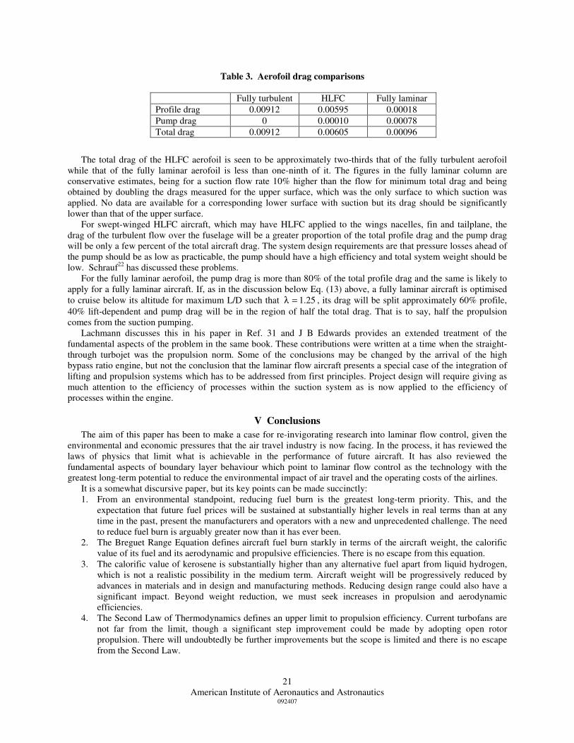
The pumping power required, divided by the free-stream velocity, is the drag arising from the suction. This so-called pump drag depends not only on the pressure losses upstream of the pump but also on the efficiency of the pump system and that of the source of the power driving the pump. It cannot be expressed as a simple function of the total suction quantity and has to be estimated carefully in each individual case. Table 3 shows illustrative profile and pump drags for the two aerofoils for which pressure distributions and boundary layer growth are shown in Figs. 13 and 14 and for the upper surface suction glove flight tested by Northrop on the F-9431, all at a Reynolds number of 30×106 approximately.


092407

21

The total drag of the HLFC aerofoil is seen to be approximately two-thirds that of the fully turbulent aerofoil

while that of the fully laminar aerofoil is less than one-ninth of it. The figures in the fully laminar column are conservative estimates, being for a suction flow rate 10% higher than the flow for minimum total drag and being obtained by doubling the drags measured for the upper surface, which was the only surface to which suction was applied. No data are available for a corresponding lower surface with suction but its drag should be significantly lower than that of the upper surface.

For swept-winged HLFC aircraft, which may have HLFC applied to the wings nacelles, fin and tailplane, the drag of the turbulent flow over the fuselage will be a greater proportion of the total profile drag and the pump drag will be only a few percent of the total aircraft drag. The system design requirements are that pressure losses ahead of the pump should be as low as practicable, the pump should have a high efficiency and total system weight should be low. Schrauf22 has discussed these problems.

For the fully laminar aerofoil, the pump drag is more than 80% of the total profile drag and the same is likely to apply for a fully laminar aircraft. If, as in the discussion below Eq. (13) above, a fully laminar aircraft is optimised to cruise below its altitude for maximum L/D such that 25.1=λ , its drag will be split approximately 60% profile, 40% lift-dependent and pump drag will be in the region of half the total drag. That is to say, half the propulsion comes from the suction pumping.

Lachmann discusses this in his paper in Ref. 31 and J B Edwards provides an extended treatment of the fundamental aspects of the problem in the same book. These contributions were written at a time when the straight-through turbojet was the propulsion norm. Some of the conclusions may be changed by the arrival of the high bypass ratio engine, but not the conclusion that the laminar flow aircraft presents a special case of the integration of lifting and propulsion systems which has to be addressed from first principles. Project design will require giving as much attention to the efficiency of processes within the suction system as is now applied to the efficiency of processes within the engine.

V Conclusions The aim of this paper has been to make a case for re-invigorating research into laminar flow control, given the

environmental and economic pressures that the air travel industry is now facing. In the process, it has reviewed the laws of physics that limit what is achievable in the performance of future aircraft. It has also reviewed the fundamental aspects of boundary layer behaviour which point to laminar flow control as the technology with the greatest long-term potential to reduce the environmental impact of air travel and the operating costs of the airlines.

It is a somewhat discursive paper, but its key points can be made succinctly: 1. From an environmental standpoint, reducing fuel burn is the greatest long-term priority. This, and the

expectation that future fuel prices will be sustained at substantially higher levels in real terms than at any time in the past, present the manufacturers and operators with a new and unprecedented challenge. The need to reduce fuel burn is arguably greater now than it has ever been.

2. The Breguet Range Equation defines aircraft fuel burn starkly in terms of the aircraft weight, the calorific value of its fuel and its aerodynamic and propulsive efficiencies. There is no escape from this equation.

3. The calorific value of kerosene is substantially higher than any alternative fuel apart from liquid hydrogen, which is not a realistic possibility in the medium term. Aircraft weight will be progressively reduced by advances in materials and in design and manufacturing methods. Reducing design range could also have a significant impact. Beyond weight reduction, we must seek increases in propulsion and aerodynamic efficiencies.

4. The Second Law of Thermodynamics defines an upper limit to propulsion efficiency. Current turbofans are not far from the limit, though a significant step improvement could be made by adopting open rotor propulsion. There will undoubtedly be further improvements but the scope is limited and there is no escape from the Second Law.

Table 3. Aerofoil drag comparisons

Fully turbulent HLFC Fully laminar

Profile drag 0.00912 0.00595 0.00018 Pump drag 0 0.00010 0.00078 Total drag 0.00912 0.00605 0.00096


092407

22

5. The greatest potential for reducing fuel burn lies in increasing aerodynamic efficiency, L/D, which means reducing drag at a given lift. The Lanchester-Prandtl induced-drag law provides the framework for assessing what is possible in increasing L/D. Structural constraints limit the potential for reducing induced drag by increasing wing span but total drag can be reduced by reducing profile drag and adjusting cruise altitude to suit. The Lanchester-Prandtl law is another constraint from which there is no escape.

6. For today’s classical swept-winged aircraft, the boundary layers are turbulent over effectively the entire surface. After 60 years of aerodynamic development the only real scope for further drag reduction of this shape lies in reducing profile drag by laminar flow control.

7. The stability of laminar boundary layers and the conditions for transition to turbulent are reasonably well understood. The stability laws define the behaviour of real fluids and, whilst again there is no escape from them, they do enable us to quantify measures that will maintain the boundary layer in a laminar state.

8. Natural and hybrid laminar flow control have the potential to reduce aerofoil and component profile drag substantially and must be serious candidates for incorporation into new aircraft designs in the medium term. Both techniques rely on the same principle, to maintain laminar flow over the forward part of the wing in order to minimise boundary layer thickness at mid chord, thereby minimising boundary layer growth and pressure drag in the rising pressure over the rear of the wing. Further research and technology demonstration is needed before either technology is sufficiently mature to be included in a new project.

9. The boundary layer equations show that, by applying suction, it is possible to maintain a laminar boundary layer in a stable condition over the full chord of a wing. Flight tests in the 1950s confirmed this. Applying overall suction to a flying wing configuration, as proposed by Handley Page in the HP 117 project, would result in profile drag lower by an order of magnitude than the profile drag of current wings. Lift to drag ratio might be increased by a factor of two or three.

10. For an all-laminar flow aircraft, approximately half the propulsive power goes into the boundary layer suction system. This is an extreme case of engine-airframe integration that will require the analysis, modelling and demonstration of all aspects of the suction system to be of the same rigour as is applied to the engine.

11. Overall, the limits set by the laws of physics lead to the conclusion that laminar flow control, in all its respects, is the most promising but also perhaps the most challenging way forward in the quest to reduce fuel burn. All other avenues to higher fuel efficiency have to be pursued in parallel but it is in laminar flow control that the greatest long-term opportunity lies – the all-laminar aircraft, with NLFC and HLFC aircraft as milestones along the road. There are many engineering and operational problems to be addressed but the underlying physics are well understood and there is a substantial body of past experience from which to draw encouragement. Looking to the environmental and economic pressures that will confront aviation in the coming decades, we must conclude that it is now time to return in earnest to the challenge of building laminar flow control into our future transport aircraft.

References 1. Intergovernmental Panel on Climate Change, IPCC Fourth Assessment Report: Climate Change 2007,

Cambridge University Press, 2007. 2. Sausen, R., Isaksen, I., Grewe, V., Hauglustaine, D., Lee, D.S., Myhre, G., Köhler, M.O., Pitari, G.,

Schumann, U., Stordal, F. and Zeferos, C. Aviation radiative forcing in 2000 : An update on IPCC (1999), Meteorol Z 14, (4) pp 555-561

3. Fahey, D.W. The Assessment of Aviation Cloudiness in IPCC Climate Change 2007 – the Physical Science Basis, ICAO Colloquium on Aviation Emissions, May 2007.

4. Green, J.E. Air Travel - Greener by Design – Mitigating the environmental impact of aviation: Opportunities and priorities, The Aeronautical Journal, September 2005, 109, (1099), pp 361-416.

5. Green, J.E. Greener by Design – the technology challenge, The Aeronautical Journal, February 2002, 106, (1056), pp 57-113.

6. Birch, N.T. 2020 Vision: The Prospects for Large Civil Aircraft Propulsion, The Aeronautical Journal, Vol. 104, No. 1038, pp 347-352, August 2000.

7. Lanchester, F.W. Aerodynamics, Constable & Co Ltd, London, 1907. 8. Ackroyd, J.A.D. Lanchester – The Man, The Aeronautical Journal, April 1992, 96, (954), pp 119-140. 9. Prandtl, L. Tragflügeltheorie, I Mitteilungen, Nach der kgl Gesellschaft der Wiss zu GööMaths-Phys, Klasse,

1918, pp451-477. 10. Küchemann, D. The Aerodynamic Design of Aircraft, Pergamon, 1978


092407

23

11. Marec, J-P. Drag Reduction: a Major Task for Research, CEAS/DragNet European Drag Reduction

Conference 2000, Potsdam, June 2000 12. Prandtl, L. Über Flüssigkeitsbewegung bei sehr kleiner Reibung, Verhandlungen des dritten internationalen

Mathematiker-Kongresses, 1904, Heidelberg, Leipzig. 13. Rayleigh, Lord (Strutt, J.W.) On the stability or instability of certain fluid motions, Proc Lond Matth Soc 11,

(1880), pp 57-70 (see also Tollmien and Grohne, Ref.30 below). 14. Tollmien, W. Über die Entstehung der Turbulenz 1. Mitteilung. Nachr Ges Wiss Gött, Math-phys Kl 1929,

pp 21-44. Translation: NACA TM No. 609 (1931). 15. Owen, P.R. and Randall, D.G. Boundary layer transition on a swept back wing, 1952, RAE Technical

Memorandum No Aero 277 and 1953, RAE Technical memorandum No 330. 16. Pfenninger, E. Some results from the X21 program. Part I: Flow phenomena at the leading edge of swept

wings, Recent Developments in Boundary Layer Research, Part IV, May 1965, AGARDograph 97. 17. Gaster, M. A simple device for preventing turbulent contamination of swept leading edges, The Aeronautical

Journal, 1965, 69, pp 788-789. 18. Gaster, M. On the flow along swept leading edges, The Aeronautical Journal, 1965, 69, p 788. 19. Poll, D.I.A. Some observations of the transition process on the windward face of a long yawed cylinder, J

Fluid Mech, 1985, 150, pp 329-356. 20. Arnal, D. Boundary layer transition. Predictions based on linear theory, April 1994, Special Course on

Progress in Transition Modelling, AGARD Report 793. 21. Wong, P.W.C. and Maina, M. Flow control studies for military aircraft applications, AIAA 2

nd Flow Control

Conference, Portland, Ore, 2004, AIAA 2004-2313. 22. Schrauf, G. Status and perspectives of laminar flow, The Aeronautical Journal, December 2005, 109, (1102),

pp 639-644. 23. Blasius, P.R.H. Grenzschichten in Flüssigkeiten mit kleiner Reibung, Z für Mathematik und Physik, 1908, 56,

pp1-37 24. Pretsch, J. Die Stabilität einer ebenen Laminarströmung bei Druckgefälle und Druckandstieg, Jb dtsch

Luftfahrtforsch, 1 (1941), pp 58-75. 25. Prandtl, L. Über Flüssigkeitsbewegung bei sehr kleiner Reibung, Verhandlungen des dritten internationalen

Mathematiker-Kongresses, 1904, Heidelberg, Leipzig. 26. Head, M.R. Methods of calculating the two dimensional laminar boundary layer, in Boundary Layer and

Flow Control, Vol. 2, Pergamon, 1961. 27. Boeing Commercial Airplane Company, Natural laminar flow airfoil analysis and trade studies, NASA

Contractor Report 159029, May 1979. 28. Bussman, K and Müntz, H. Die Stabilität der laminaren Reibungsschicht mit Absaugung, Jb dtsch Luftfahrt,

1, (1942) pp 1-7. 29. Ashill, P.R., Wood, R.F. and Weeks, D.J. An Improved, Semi-Inverse Version of the Viscous Garabedian

and Korn Method (VGK), RAE TR 87002, 1987. 30. Schrauf, G. and Kühn, W. Indusatrial aspects of laminar flow, presented at EC Fourth Aeronautics Days,

Hamburg, Germany, January 2001. 31. Lachmann, G.V. (Ed.) Boundary Layer and Flow Control, Vol. 2, Pergamon, 1961. 32. Maddalon, D.V. and Braslow, A.L. Simulated-Airline Service Flight Tests of Laminar-Flow Control with

Perforated-Surface Suction System, NASA Technical Paper 2966, Washington DC, March 1990. 33. Braslow, A.L. A History of Suction-Type Laminar-Flow Control with Emphasis on Flight Research, NASA

History Division, Monographs in Aerospace History No. 13, Washington DC, 1999.

laminar flow control: back to the future? (invited)

Documents