LAKE EVAPORATION ESTIMATION IN ARID ENVIRONMENTS

FINAL REPORT

by

W.E. Eichinger, J. Nichols, J.H. Prueger, L.E. Hipps, C.M.U. Neale, D.I. Cooper, and A. S. Bawazir

Sponsored by

U.S. Bureau of Reclamation

IIHR Report No. 430

IIHR - Hydroscience & EngineeringThe University of Iowa

Iowa City IA 52242-1585

July 2003

TABLE OF CONTENTS

I. STATEMENT OF THE PROBLEM. . . . . . . . . . . . . . . . . . . . . . . . . . . . . . . . . . . . . . 1II. ELEPHANT BUTTE RESERVOIR. . . . . . . . . . . . . . . . . . . . . . . . . . . . . . . . . . . . . . 1

A. Measurements at Elephant Butte Reservoir . . . . . . . . . . . . . . . . . . . . . . . . . .4 B. Instruments. . . . . . . . . . . . . . . . . . . . . . . . . . . . . . . . . . . . . . . . . . . . . . . . . . . .4III. EVAPORATION ESTIMATION. . . . . . . . . . . . . . . . . . . . . . . . . . . . . . . . . . . . . . .6

A. Traditional Estimates of Evaporative Fluxes . . . . . . . . . . . . . . . . . . . . . . . .6B. Monin Obukov Similarity Method.. . . . . . . . . . . . . . . . . . . . . . . . . . . . . . . . .9C. Required Instrumentation . . . . . . . . . . . . . . . . . . . . . . . . . . . . . . . . . . . . . .10D. Uncertainty of the Proposed Method . . . . . . . . . . . . . . . . . . . . . . . . . . . . . 11

IV. RESULTS FROM ELEPHANT BUTTE . . . . . . . . . . . . . . . . . . . . . . . . . . . . . . . . 13V. COMPARISON TO PAN MEASUREMENTS . . . . . . . . . . . . . . . . . . . . . . . . . . . 18VI. CONCLUSIONS . . . . . . . . . . . . . . . . . . . . . . . . . . . . . . . . . . . . . . . . . . . . . . . . . . . 20VII. BIBLIOGRAPHY . . . . . . . . . . . . . . . . . . . . . . . . . . . . . . . . . . . . . . . . . . . . . . . . . .22APPENDIX 1. MONIN OBUKHOV METHOD . . . . . . . . . . . . . . . . . . . . . . . . . . . . . . .24APPENDIX 2. AVAILABLE DATA SETS. . . . . . . . . . . . . . . . . . . . . . . . . . . . . . . . . . 26

LIST OF TABLES

Table 1. Instruments Mounted on the Meteorological Tower at Elephant Butte. . . . . . . . . 4Table 2. Recommended Instruments for Open Water Measurement Sites. . . . . . . . . . . . 11

LIST OF FIGURES

Figure 1. An overhead photograph of the peninsula upon which the experiment wasconducted. . . . . . . . . . . . . . . . . . . . . . . . . . . . . . . . . . . . . . . . . . . . . . . . . . . . . . . . . . . . . . . 3

Figure 2. The meteorological instrument tower at Elephant Butte and the view to the north-east. . . . . . . . . . . . . . . . . . . . . . . . . . . . . . . . . . . . . . . . . . . . . . . . . . . . . . . . . . . . . . . . . . . . 5

Figure 3. A closeup photograph of the meteorological tower showing the instrumentsmounted on it. . . . . . . . . . . . . . . . . . . . . . . . . . . . . . . . . . . . . . . . . . . . . . . . . . . . . . . . . . . . 5

Figure 4. A plot of the temperature at various depths at the tower site in Elephant Butte fora period of ten days following the intensive campaign. . . . . . . . . . . . . . . . . . . . . . . . . . . . . 6

Figure 5. A plot of the temperature at various depths at the tower site in Elephant Butte overthe course of a day. . . . . . . . . . . . . . . . . . . . . . . . . . . . . . . . . . . . . . . . . . . . . . . . . . . . . . . . 7

Figure 6. A plot of evaporation rate over Elephant Butte during the intensive campaign. . 8

Figure 7. A plot showing the evaporation rate at Elephant Butte during the last quarter of2001. . . . . . . . . . . . . . . . . . . . . . . . . . . . . . . . . . . . . . . . . . . . . . . . . . . . . . . . . . . . . . . . . . . . 8

Figure 8. A plot of the eddy covariance rate determined by the Monin-Obukhov method andthat determined by eddy covariance over the intensive period. . . . . . . . . . . . . . . . . . . . . . . 13

Figure 9. A plot of the eddy covariance rate determined by the Monin-Obukhov methodversus that determined by eddy covariance. . . . . . . . . . . . . . . . . . . . . . . . . . . . . . . . . . . . . . .14

Figure 10. A comparison of the evaporation estimates of the Monin-Obukhov method andthose obtained from the eddy covariance instruments for days 266 through 365 of 2001. . 14

Figure 11. A comparison of the daily average evaporation estimates of the Monin-Obukhovmethod and those obtained from the eddy covariance instruments for days 266 through 365of 2001. . . . . . . . . . . . . . . . . . . . . . . . . . . . . . . . . . . . . . . . . . . . . . . . . . . . . . . . . . . . . . . . 15

Figure 12. A comparison of the vertical momentum flux, (u*) estimates from the Monin-Obukhov method and those obtained from the eddy covariance instruments for days 266through 365 of 2001. . . . . . . . . . . . . . . . . . . . . . . . . . . . . . . . . . . . . . . . . . . . . . . . . . . . . . .15

Figure 13. a.) A comparison of the measured and estimated evaporation rates over a 8 dayperiod. b.) The surface and air temperatures and humidities and c.) The wind speed anddirection. . . . . . . . . . . . . . . . . . . . . . . . . . . . . . . . . . . . . . . . . . . . . . . . . . . . . . . . . . . . . . . 17

Figure 14. A plot of the measured evaporation rate, the proposed estimation method and thetwo pan estimates. . . . . . . . . . . . . . . . . . . . . . . . . . . . . . . . . . . . . . . . . . . . . . . . . . . . . . . . 19

Figure 15. A plot of the pan evaporation estimates vs the measured evaporation rate. . . . 20

Figure 16. Flow chart of Monin-Obukhov method using meteorological data. . . . . . . . . 25

1 IIHR - Hydroscience & Engineering, Iowa City, IA2 USDA Soil Tilth Laboratory, Ames, IA3 Utah State University, Logan, UT4 Los Alamos National Laboratory, Los Alamos, NM5 New Mexico State University, Las Cruces, NM

1

LAKE EVAPORATION ESTIMATION IN ARID ENVIRONMENTS

Final Report

by

W. Eichinger1, J. Nichols1, J. Prueger2, L. Hipps3, C. Neale3, D. Cooper4, and A.S. Bawazir5

I. STATEMENT OF THE PROBLEM

Open water evaporation is a currently undetermined loss to the Rio Grande. The Rio

Grande provides 97 percent of the water needed in the New Mexico Rio Grande Basin

[Hansen, 1996]. As a result of rapid urban and industrial growth, there has been a 35 percent

increase in municipal and industrial water use in the corridor from Taos to Las Cruces, NM

over the past fifteen years. To compound the problem, it is expected that the water demand

in the Rio Grande Valley will more than double over the next fifty years. This growth

compounds an existing water problem and adds to the urgency for improved water efficiency

and effective long-term planning efforts [Berger, 1997]. Current water management

techniques that regulate the flow in the river rely on water budgeting that, in addition to

satisfying local needs, must guarantee a certain water level in the river (due to the endangered

status of the Rio Grande silvery minnow) and a mandated quantity of water leaving New

Mexico (to comply with water agreements with Mexico and Texas). Too little water released

from reservoirs results in economic loss downstream and legal action, while too much water

released is, from the point of view of New Mexico, essentially wasted.

The existing data on water use are incomplete and often contradictory. Agricultural

use accounts for about 80 percent of the surface flow diverted from the Rio Grande

(~100,000 acre-feet per year [Hansen and Gould, 1998]), but less than 20 percent of the

known losses from the river (most of the diverted water is returned). Water evaporated from

open-water surfaces is believed to constitute the major loss from the hydrologic budget of

2

the basin. Estimates of evaporative losses range from 230,000 [Hansen and Gould, 1998]

to 350,000 [Wilson, 1997] acre feet per year. The evaporative losses from the Elephant

Butte Reservoir alone have been estimated to be 140,000 acre-ft per year, with a high of

228,000 acre-ft and a low of 41,000 acre-ft per year [Action Committee of the Middle Rio

Grande Water Assembly, 1999]. The wide range of current evaporation estimates makes

accurate estimation and forecasting a critical management need. Estimates of losses from

seepage into the ground range from 8 to 12 percent of the total losses. If evapotranspiration

could be well estimated, it would quantify the open water losses and the bulk of the use by

agriculture and riparian vegetative areas (estimated as 136,000 acre-feet per year [Hansen

and Gould, 1998]). This hydro-ecological process has been modeled in only a rudimentary

way, using fragmented and out-dated quantitative data over the region. Current methods for

evaporation estimation (pans, Blaney-Criddle, Penman-Monteith, etc) are not sufficiently

accurate to enable precision water planning or to suggest improved management methods.

As an example, using the current Bureau of Reclamation model (a modified Penman-

Monteith), it is impossible to state definitively whether non-native salt cedar uses more or

less water than the native cottonwood trees along extensive reaches of the Rio Grande basin.

The traditional methods of evaporation estimation are not only inaccurate, but do not

provide the ability to improve the quality of the evapotranspiration estimates. They lack the

physical and biological knowledge that represent the actual environment on the Rio Grande.

This preliminary report presents the results of a multi-disciplinary, multi-agency

collaborative effort to measure, characterize, and improve modeled open water evaporation

from Elephant Butte Reservoir.

The ability to accurately estimate water evapotranspiration is the key element

required to make further improvements in water management. The ability to accurately

estimate evapotranspiration in the area along the Rio Grande would allow accurate

calculation of water use by riparian and agricultural areas (which constitute the majority of

the demand for water) as well as open water losses in the Rio Grande basin. This in turn will

allow more effective use of available water resources. Further, accurate estimation of the

losses provides a basis upon which planning can occur to reduce these losses. Sustainable

agriculture in the presence of a rapidly growing water demand depends upon more efficient

water use.

3

Figure 1. An overhead photograph of the peninsula upon which theexperiment was conducted. The tower and lidars were located at theend (upper right corner). This location put the instruments near thecenter of the lake with a minimum of interference from dry land.

II. ELEPHANT BUTTE RESERVOIR

Elephant Butte Reservoir is a large reservoir in the middle Rio Grande Valley that

runs north-south through the center of New Mexico. The reservoir itself is roughly 60 km

long and 2 to 4 km wide, running north to south, with a total volume of 2.22 million acre-feet

of water. This reservoir is surrounded by a semi-arid region with an average annual

precipitation between 7 inches and 15 inches over two thirds of the Rio Grande Basin, from

San Marcial - Elephant Butte Dam to Radium Springs. Precipitation exceeds 25 inches only

where 30 to 75 percent of the annual precipitation is in the form of snow, while in the

balance of the watershed snow represents less than 25 percent of the annual precipitation.

The vegetation in the area is primarily mature saltcedar that grows in the low lying areas that

drain into the lake. The area also includes a limited amount of cottonwood trees, creosote

bushes, and mesquite. The Fra Cristobal Mountain Range parallels the eastern and southern

part of the reservoir. The western side consists of sediment deposits from the Rio Grande.

With a maximum surface area of 36,500 acres, the evaporative losses from the lake are a

significant component of the water budget of the region.

The storage content of Elephant Butte Reservoir at the beginning of the year, on

December 31, 1999, was 1,708,200 ac-ft at an elevation of 4396.58 feet. The storage content

at the end of 2000, was projected to be 1,250,810 at an elevation of 4,380.39 feet. Elephant

Butte Reservoir releases for 2000 are estimated to be 801,000 ac-ft.

In order to measure

evaporative losses from the

reservoir, an instrumented

tower was placed at the end

of a long, narrow spit of land

that extended into the lake

(figure 1) (N 33:19.114,

W107:10.383). This location

allowed placement of the

tower in more than 25 ft of

water in a central location in

the reservoir. The instruments

4

had minimum interference from dry land. The tower was erected in July 2001 and remained

in place until April 2002 when the water level in the reservoir dropped to the point where the

tower was on dry land. A list of the instruments mounted on the tower is provided in table

1. A listing of the available data is contained in appendix 2.

A. Measurements at Elephant Butte Reservoir. In order to measure the

evaporation from Elephant Butte Reservoir, a set of hydrological and meteorological sensors

were fielded in 2001 in the north-central portion of the lake. An intensive measurement

campaign was conducted from 12 to 24 September 2001. This campaign included the Los

Alamos National Laboratory (LANL) scanning Raman lidar, a sodar, as well as high

frequency, time series measurements of the instruments on the tower.

Table 1. Instruments Mounted on the Meteorological Tower at Elephant Butte

Instrument Height Above the Water Measures

CSAT3, Sonic

Anemometer

3.62 m Wind speed, direction, turbulent

quantities

KH20, Krypton

Hygrometer

3.62 m Water vapor concentration fluctuations

HMP45C, Temp-Humidity

Probe

2.5 m Atmospheric temperature and humidity

Q7.1, Net Radiometer 4.50 m Net long and short wave radiation

MET ONE 34A-L, Cup

Anemometer and Vane

5.5 m Wind direction

Infrared Thermometer 4.5 m Lake surface temperature

Thermocouple Array 15, 27, 47, 83, 147 cm depths Lake temperature at various depths

B. Instruments. The instruments shown in figures 2 and 3 comprise an

energy/water budget and meteorological flux station. The water/energy budget is composed

of measurements of net radiation and heat storage (available energy), and turbulent fluxes

of sensible and latent heat, as well as the momentum flux. The available energy is measured

by a net radiometer, and a vertical water temperature profile that is used to compute the

amount of thermal energy stored in a water column. The sensible, latent heat (evaporation)

5

Figure 3. A closeup photograph of the meteorologicaltower showing the instruments mounted on it.

Figure 2. The meteorological instrument tower atElephant Butte and the view to the north-east.

and momentum fluxes were measured with a sonic anemometer and a fast response

hygrometer.

The sonic anemometer measures the three dimensional components of the wind flow

(u, v, and w, the three components of the wind speed) at high rates, up to 20 Hz. These wind

observations were used to compute the vertical transport term of the eddy covariance fluxes.

The krypton hygrometer measures the fluctuations of atmospheric water vapor concentration

(q’) at the same rate as the sonic anemometer (20 Hz). Together, the fluctuations in the

vertical wind speed (w’) and water vapor concentration (q’) about their mean values were

used to calculate the evaporative flux from the lake as , where the overbar indicates

time averaging. The covariance of these variables is the “standard” reference for flux

determination (subject to various corrections for instrument limitations [Webb et al., 1980;

Massman, 2000; Massman and Lee, 2002]). This method is accepted as the most physically

based technique to measure evaporation and was used in this project as the “truth set”. The

6

23 24 25 26 27 28 29 30 31 32

Twat

er (D

eg C

)

236 238 240 242 244 246 248 DOY

15 cm 27 cm 47 cm 83 cm 147 cm

Elephant Butte 2001

Figure 4. A plot of the temperature at various depths at thetower site in Elephant Butte for a period of ten days followingthe intensive campaign.

(1)

temperature/humidity probe is used as part of a standard meteorological station that will be

used as a data set for evaluating the utility of more advanced models for estimating

evaporative flux from the lake.

III. EVAPORATION ESTIMATION

A. Traditional Estimates of Evaporative Fluxes. Over land, the sun deposits its

energy in the top few millimeters of the surface. The land surface modulates its temperature

so as to partition outgoing energy (sensible and latent heat fluxes, soil heat flux, and outgoing

long-wave radiation) in a way that satisfies the physical requirements of the situation. If the

surface has vegetation, the system increases in complexity. Depending on the amount of

water available, the incoming energy

will tend to partition in favor of

evaporation. In contrast, over

sparsely vegetated arid environments,

the partitioning will tend to favor the

sensible heat flux. The availability

of water near the surface will also

govern this partitioning. In general,

the energy that drives evaporation

comes from and is directly

proportional to the available

radiation. At night the evaporation

rates drop dramatically, although not

necessarily to zero, because of heat stored in the ground and from the air itself. At night, a

land surface will cool more rapidly than the air, with the result that energy will be extracted

from the air to support evaporation. Many of the commonly used, traditional estimates of

evaporation (Penman, Penman-Monteith, Priestly-Taylor, etc.) rely on the proportionality

between the evaporative flux and the available radiation.

The Penman equation (Eq. 1.) forms the basis for most of the traditional methods

7

-3.00

-2.50

-2.00

-1.50

-1.00

-0.50

0.0024 25 26 27 28 29 30 31

Temperature (Deg C)

Dep

th (m

)0730 hrs1030 hrs1330 hrs1630 hrs

Aug. 25 2001

Figure 5. A plot of the temperature at various depths at thetower site in Elephant Butte over the course of a day. Notethat the lake temperature below about 1.5 m does not changesignificantly during the day.

where � = desat / dT (the slope of the saturation vapor pressure curve with temperature); �

is the psychometric constant, � = Cp P / 0.622 Le; Cp is the specific heat, at constant

pressure, of dry air; P is the atmospheric pressure; Le is the latent heat of vaporization for

water; Rn is the net radiation; G is the storage term; ƒ is an empirical wind function; and (esat

- ea) is the water vapor pressure deficit in the atmosphere.

Fundamentally, the physics used to derive this semi-empirical model assumes that

evaporation is driven by the

available energy and the vapor

pressure deficit. However, it is

well-known that the available

energy over water is only weakly

related to evaporation (Sellers,

1965). This will be demonstrated

later in this section. Further, the

empirical wind function is site

specific, and is affected by the slope

of the terrain and the height and

variability of the roughness elements

at the surface. In practice, near

surface stability also affects the wind function, and but is typically not included in the

derivation and handled with empirical “work arounds”. In short, substantial errors and

uncertainties should be anticipated if this approach is used for estimating open water

evaporation.

With respect to evaporation, open water bodies are quite different from land surfaces.

The sun’s energy penetrates the water to depths of as much as 30 m in clear water, somewhat

less in turbid water, and is stored throughout the water column. The water column is mixed

by surface motion and becomes the source of energy that drives evaporation. Because of the

large heat storage capacity of water (1.006x106 J/m3), and the fact that water is approximately

1000 times more dense than air, the temperature of deep, clear, water bodies does not change

significantly throughout the day when compared to the atmosphere (see figure 4 for

example). The amount of available energy at the surface is nearly constant throughout the

8

Figure 7. A plot showing the evaporation rate at Elephant Butte duringthe last quarter of 2001. The red line is a daily running average of theevaporation rate. The high portions of the red line are the result ofstorms with high winds over the reservoir.

-200

0

200

400

600

800

1000

260 261 262 263 264 265 266 267

DOYLE

(W/m

-2)

Sep 17-24 2001

Figure 6. A plot of the evaporation rate over Elephant Butte duringthe intensive campaign. Note that the rate is essentially constantand does not follow a diurnal cycle ( the highs and lows areindicative of changes in wind speed). The one period over 800W/m2 occurred during a convective storm.

day and night, leading to a nearly

constant evaporation rate (figure

6). The water in Elephant

Butte Reservoir lies between the

two extremes of a clear water

body and a land surface. The

lake is shallow over much of its

area and is relatively turbid,

resulting in massive storage of

solar energy in a considerably

smaller volume. The bulk

temperature of the lake (the

temperature below about a half

meter) will fluctuate to a small

degree over the course of a day (figure 5) and the evaporation rate will change with it.

Methods that use net radiation to estimate evaporation rates must fail, because net

radiation is not providing the energy required for evaporation. For example, these models

(Eq. 1) will predict a small or zero evaporation rate at night since Rn is small. Over a water

body at night, the evaporation rate is in fact, nearly as large as it is during the day. Figure 6

shows the evaporation at the tower during the intensive period. The evaporation rates are

n e a r l y c o n s t a n t a t

approximately 100 W/m2.

The variations observed in

Figure 6 are primarily the

result of changes in wind

speed. Periods of near zero

evaporation are actually

periods when the winds blow

from the north, through the

tower before reaching the

eddy covariance instruments,

and are instrument artifacts in

9

(2a)

the “truth” set. Even on a daily or weekly basis, conventional methods based on net radiation

will not work well. For example, between April and July, the lake temperature will rise

significantly as an extremely large amount of energy is stored in the water. Methods that use

the net radiation will assume that all of the available energy is going into sensible or latent

energy, yet a significant portion is used to warm the lake. On a daily basis, the overestimate

of evaporation is not large but is consistently an overestimate, and over a large lake over

several months, the amount of error continually accumulates. Similarly, in the fall as the lake

cools, these methods will underestimate the evaporation rates. Figure 7 is a plot showing all

of the evaporation data collected at the tower during 2001. While the individual evaporation

rates are quite scattered, the running average over a 24 hour period is relatively constant.

The average over the entire period is 92 W/m2 (equivalent to 3.26 mm/day). Note that the

daily evaporation rate decreases slightly in December. The decrease is associated with

westerly winds with smaller velocities (and unusually small momentum fluxes).

An alternative to these traditional methods relies upon the fact that the evaporation

rate is known to be proportional to the water vapor deficit above the water surface and to the

wind speed (or more precisely, the vertical momentum flux, u*). While bulk methods using

this approach exist, we suggest the use of similarity theory that accounts for atmospheric

stability in a more direct way.

B. Monin Obukov Similarity Method Over ideal homogeneous surfaces,

Monin-Obukhov Similarity (MOS) Theory relates changes of vertical gradients in wind

speed, temperature, and water vapor concentration. According to MOS Similarity Theory,

the relationship between the temperature and water vapor concentration at the surface, Ts and

qs, and the wind speed, u(z), temperature, T(z), or water vapor concentration, q(z), at any

height, z, within the inner region (first few meters of atmosphere above the surface) of the

boundary layer is expressed as

10

(2b)

(2c)

(3)

Where the Monin-Obukhov length, L, is a stability parameter, defined as:

zo is the roughness length (and is assumed to be the same for all variables), H is the sensible

heat flux, LE is the latent energy flux, � is the density of air, Le is the latent heat of

evaporation for water, cp is the specific heat for air, k is the von Karman constant (taken at

0.40), u* is the friction velocity, g is acceleration due to gravity, and �m, �h, and �v are the

Monin-Obukhov stability functions for momentum, temperature and water vapor.

Simply, the MOS method assumes that vertical fluxes of scalars and mass are

proportional to the difference between values at the surface and some height, z, and scaled

by a term that quantifies the turbulent transport, the friction velocity, u*. The method is

simple, requiring only a measure of wind speed, temperature and humidity at some height

and the temperature at the water surface (the air immediately above the lake surface is

assumed to be saturated). At the surface, the wind speed is zero since the kinetic energy of

the wind is transferred to the water in the form of waves.

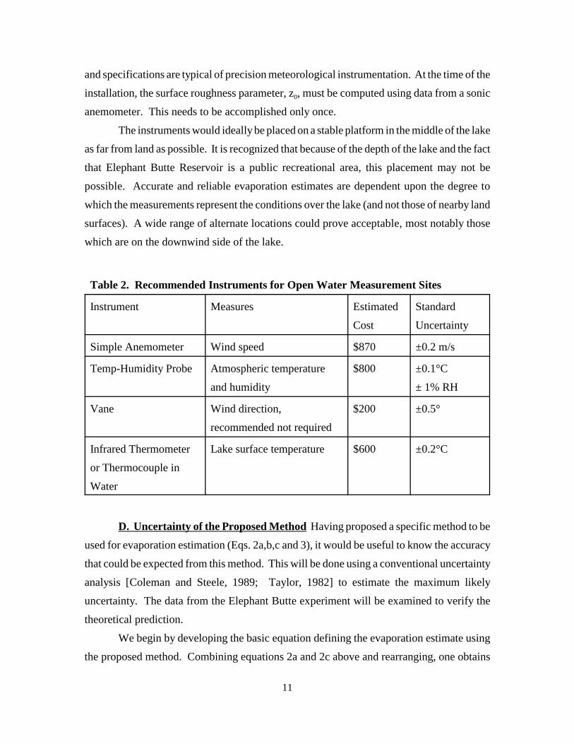
C. Required Instrumentation. Because of the simplicity of the Monin-Obukhov

method, no complex instruments are required. Indeed, the instruments needed are little more

than a conventional meteorological station. At an appropriate height above the water surface,

required measurements are air temperature, humidity, and wind speed. A measurement is

also needed of the lake temperature near the surface. This could be done with an infrared

thermometer mounted on a mast with the other instruments or with a thermocouple placed

near the water surface. Table 2 contains a summary of the suggested instruments. The costs

11

and specifications are typical of precision meteorological instrumentation. At the time of the

installation, the surface roughness parameter, z0, must be computed using data from a sonic

anemometer. This needs to be accomplished only once.

The instruments would ideally be placed on a stable platform in the middle of the lake

as far from land as possible. It is recognized that because of the depth of the lake and the fact

that Elephant Butte Reservoir is a public recreational area, this placement may not be

possible. Accurate and reliable evaporation estimates are dependent upon the degree to

which the measurements represent the conditions over the lake (and not those of nearby land

surfaces). A wide range of alternate locations could prove acceptable, most notably those

which are on the downwind side of the lake.

Table 2. Recommended Instruments for Open Water Measurement Sites

Instrument Measures Estimated

Cost

Standard

Uncertainty

Simple Anemometer Wind speed $870 ±0.2 m/s

Temp-Humidity Probe Atmospheric temperature

and humidity

$800 ±0.1°C

± 1% RH

Vane Wind direction,

recommended not required

$200 ±0.5°

Infrared Thermometer

or Thermocouple in

Water

Lake surface temperature $600 ±0.2°C

D. Uncertainty of the Proposed Method Having proposed a specific method to be

used for evaporation estimation (Eqs. 2a,b,c and 3), it would be useful to know the accuracy

that could be expected from this method. This will be done using a conventional uncertainty

analysis [Coleman and Steele, 1989; Taylor, 1982] to estimate the maximum likely

uncertainty. The data from the Elephant Butte experiment will be examined to verify the

theoretical prediction.

We begin by developing the basic equation defining the evaporation estimate using

the proposed method. Combining equations 2a and 2c above and rearranging, one obtains

12

(4)

(5)

(6)

(7)

where all of the variables are as defined above. To simplify the analysis, the atmosphere is

assumed to be neutral, i.e. �m and �v the stability corrections functions are zero. This

assumption greatly simplifies the analysis without loss of generality. With this assumption,

the evaporation estimate becomes

Using error propagation methods, assuming the measurements are independent (although the

relative humidity measurement is not independent of the temperature), and that the fractional

uncertainty in air density is equal to the fractional uncertainty in temperature, the fractional

uncertainty in the evaporation rates is obtained by summing the contributions in quadrature:

where the � indicates the uncertainty in the value that follows the symbol.

Assuming a typical air temperature of 27°C, a relative humidity of 23%, a wind speed

of 2.5 m/s, a lake surface temperature of 23°C, a measurement height of 3 m and an

uncertainty in z0 of 25% from our measured value during of the intensive campaign of

0.00055 m, and using the manufacturer’s estimates for the uncertainty of the instruments, the

following estimate for the fractional uncertainty can be obtained:

This estimate of the uncertainty is somewhat deceptive. It assumes a perfect surface

and ideal conditions (in other words, it assumes that the theory completely and perfectly

13

Figure 8. A plot of latent heat flux measured with eddy covariance andcomputed using the Monin-Obukhov method over the intensive period.

describes the phenomena). Elephant Butte Reservoir is a narrow lake in the middle of an arid

region and far from ideal. The influence of advection (hot dry air from land) on the local

evaporation rate cannot be discounted. This is especially true depending on from what

direction the wind is blowing, particularly winds with easterly or westerly components.

IV. RESULTS FROM ELEPHANT BUTTE

In order to estimate how well the proposed method determines evaporative losses

over the lake, we will use the data already taken over the lake just as one would if the

concept was implemented.

There is one free parameter

that must be evaluated; the

surface roughness parameter,

z0. We will use the data from

the intensive campaign that

was conducted from 12 to 24

September 2001 to determine

this parameter and then apply

it to the remainder of the data

to determine the effectiveness of the method.

During the intensive period, eddy covariance measurements were recorded at20 Hz.

The evaporation rates derived from the eddy covariance method is taken as the truth set from

which the roughness parameter is derived. The method described in appendix 1 is used to

analyze the data. The roughness parameter is optimized by requiring the minimum rootmean

square difference between the Monin-Obukhov derived evaporation rates and the eddy

covariance derived evaporation rates to be a minimum. This criterion was developed so that

the MOS method is as accurate as possible on a short term basis, not just as a monthly

average. The time-series of 30 minute latent energy fluxes from both the eddy covariance

instruments and the MOS model is shown in figure. 8. Figure 9 shows the comparison

between “filtered” MOS derived evaporation fluxes versus the eddy covariance fluxes during

the intensive period.

14

Figure 9. A plot of the eddy covariance rate determined by theMonin-Obukhov method versus that determine by eddycovariance. The RMS difference between the two methods is41 W/m2.

Figure 10. A comparison of the evaporation estimates of theMonin-Obukhov method and those obtained from the eddycovariance instruments for days 266 through 365 of 2001. Data was excluded if the wind was coming from within 30° ofnorth.

When the wind is from the

north, it must pass through the tower

that holds the sonic anemometer.

This creates artificial turbulence that

distorts the measured evaporation

rate. Because of this, all of the data

within 30 degrees of north was

filtered and eliminated from the data

set. Using an iterative best-fit

technique, the optimized value of the

roughness parameter is 7x10-5m.

This produces a root mean square

difference between the values of the evaporation rates of 41 W/m2 during the intensive

period. Over the duration of the intensive period, the total evaporation, as determined by the

eddy covariance method, is 15.86mm and that by the proposed method 17.07mm. The

difference between them is approximately 7.6%, a value consistent with the theoretical

analysis above.

The value of the roughness parameter determined for the intensive campaign was

applied to the data measured at the tower site for the rest of the year, days 266 through 365

of 2001. A comparison of the estimated evaporation rates and the measured evaporation is

shown in figure 10. The differences between the measured and estimated values are in some

cases much larger than in figure 9.

The RMS difference between the

measured and estimated values is 58

W/m2. However, as can be seen in

figure 11, the difference between the

daily average evaporation rates is

much smaller. Over this period, the

average measured evaporation rate

was 92.6 W/m2 and the estimate is

94.6 W/m2. The RMS difference

between the daily averages is 8.4

15

Figure 11. A comparison of the daily average evaporationestimates of the Monin-Obukhov method and those obtained fromthe eddy covariance instruments for days 266 through 365 of 2001. The green line is the estimate and the red is the measured.

Figure 12. A comparison of the vertical momentum flux, (u*) estimatesfrom the Monin-Obukhov method and those obtained from the eddycovariance instruments for days 266 through 365 of 2001. The blackline indicates a one to one correspondence.

W/m2, which is consistent with

the theoretical prediction. It

would be fair to say that while the

individual measurements may be

significantly in error, the average

estimates over periods as short as

a day are quite accurate.

The reason for this

behavior can be seen in figure 12.

This is a comparison of the

measured and estimated vertical

momentum flux, u*, also known as the “friction” velocity. The black line indicates a one to

one comparison. There may be as many two other common relationships that apply. This

could be the result of two different processes. The first is the result of differences in wind

direction. Winds blowing from the west will have different turbulent characteristics than

winds blowing along the lake, from the north or south. Similarly, winds from the east,

blowing over the bluffs will have different turbulent characteristics as well. This is

especially true as the reservoir contracted (due to drought conditions) during these months;

the influence of the nearby land surface should have been increasingly pronounced. The

method, as implemented,

assumes no directionality.

The surface roughness

of a water body changes as

the wind speed increases (i.e.

the waves get larger). Thus

the roughness parameter, z0,

should be a function of the

wind speed. For most

common wind velocities, the

adjustments are minimal.

However, as the wind speed

becomes large, the surface

16

roughness also increases, increasing the vertical momentum flux (and the estimated

evaporation rate). As can be seen in figure 12, the method seriously underestimates the

momentum flux when the momentum flux is large. As an academic exercise, methods could

be developed to adjust the values of the surface roughness based on wind speed and

direction. However, in a practical sense, attempting to increase the accuracy of the method

below 8 % is probably a wasted effort as the comparison “truth” set is not accurate to better

than about 10 %. Given the variability of the depth of the reservoir (and thus the area it

covers), the influence of the surrounding land surfaces is quite variable.

These phenomena can be seen in figure 13, which shows the traces of all of the

relevant data over an eight day period following the intensive campaign. The top graph is

a comparison of the measured and estimated fluxes. Those times when the differences

between the measured and estimated evaporation rates are greatest occur when the measured

fluxes are near zero or at their largest. The periods with high evaporation rates (time

increments 170, 220, and 270) are associated with high wind speeds. While the surface and

air temperatures and humidities vary in a regular fashion, little occurs that would cause large

variations in the estimated evaporation. The periods with near zero measured evaporation

rates (time increments 100, 150, 200, and 250) are associated with wind directions near zero

or 360° (north). As mentioned previously, these are an instrument artifact due to the

presence of the tower. Note that the proposed method estimates evaporation rates during

these periods that are more realistic than the eddy covariance method.

On a theoretical basis there is an issue with the treatment of z0 as applied here.

Strictly speaking, the appropriate gradient of specific humidity should be between the height

of the roughness length for water vapor and the height, z, where the temperature and

humidity measurements are made. The specific humidity at the lower level is an

aerodynamic humidity, analogous to the aerodynamic temperature. Since aerodynamic

humidity measurements a few millimeters above a waving water surface cannot really be

known, the humidity at the water surface is used instead. This approach has been attempted

for heat, using the radiometric temperature with inconsistent results. Adjustments have been

attempted, adding an excess resistance, or redefining the roughness length to account for

choosing the wrong boundary condition. However, research done with sensible heat fluxes

have never really resolved this issue. This issue is important when the surface has a

significant canopy, where the surface temperature is somewhat ambiguous and

17

Figure 13. a.) A comparison of the measured and estimated evaporation rates over a 8 day period. b.) Thesurface and air temperatures and humidities and c.) The wind speed and direction. Note that the periods oflarge disagreement between the measured and estimated fluxes are periods of high winds.

18

where the height, z0, is significant. Over a reservoir such as Elephant Butte, the estimated

value of z0 is a fraction of a millimeter, so the difference between the specific humidity at the

surface and at the height, z0, is minimal.

In order for water management efforts to be effective, decision making must be

accomplished on time scales of approximately a week (or the time it takes for water to travel

the distances between the major reservoirs). Thus estimation methods must be accurate on

time scales shorter than that to be effective or useful. Further, the methods used should be

predictive. The fact that the proposed method can be used with weather prediction data to

project the evaporation estimates into the future to be a major advantage.

V. COMPARISON TO PAN MEASUREMENTS

Pan evaporation is one of the oldest and simplest methods of measuring open water

evaporation with continuous measurements in some places dating back nearly 120 years.

The measurement involves placing a pan in open area and measuring how much water

evaporates during a period of time. The amount of evaporation as measured from the pan

is used to estimate the actual evaporation over an area through the use of a coefficient known

as the “pan coefficient, (Kp)”. Evaporation pans are commonly used to estimate lake

evaporation as Elake = Kp Epan , where Elake is the lake evaporation and Epan is the pan

evaporation. A limitation of this methodology is that the pan coefficient is considered to be

dependent on the local environment around the pan, the type and size of pan used, and on the

manner in which the pan is operated and managed. It is well-known that pan evaporation

differs from lake evaporation for a number of reasons. These factors have been outlined by

Dingman (2002) and include the difference in the heat-storage capacity of the pan, the lack

of surface-or ground-water sources, and, with raised pans, energy transfer from the sides

exposed to the air and sun. The pan coefficient used by the Bureau of Reclamation is 0.7.

Data from two Class A pans are available. One was located on a bluff at the south

end of the reservoir. The other was located at Monticello point, just to the south-west of the

tower site. The manufacturer of the pans (BCP electronics) estimates the resolution for the

automated pan at 0.1mm (0.004in). Because of the way the instrument functions, when the

amount of rainfall was greater than 10mm, the total pan evaporation was recorded as 0 mm

(no evaporation) while days in which the rainfall was less than 10mm pan the evaporation

19

Figure 14. A plot of the measured evaporation rate, the proposed estimation method and the two panestimates. Because of solar heating of the pan, the pan estimates for the summer months is nearly twice theactual rate.

was recorded as less than 0.5mm/day.

A comparison of the pan evaporation estimates is shown in figure 14. The agreement

appears to be quite good in the last part of the measured period. However, the pans greatly

overestimate the evaporation in the summer months. This is because the pans have a small

albedo and are not connected to the ground. They absorb a great deal of solar energy during

the day, making the water in the pan quite warm. The higher water temperature increases the

vapor deficit over the pan and thus the amount of water that evaporates from the pan. The

consistent overestimation of the evaporation can be seen in figure 15. Over this period, the

average measured evaporation rate was 92.6 W/m2 , that from the proposed method was 94.6

W/m2 ( difference), that from the south pan is 140.9 W/m2 and that from the pan on

Monticello point was 116.8 W/m2. The RMS difference between the daily average of the

proposed method and the measured evaporation is 8.4 W/m2, while the RMS differences

between the pan estimates and the measured evaporation is 68.7 W/m2 (South end) and 45.8

W/m2 (Monticello Point). The long term pan measurements greatly overestimate the amount

of evaporation, especially during the summer. On a daily basis, the average error is on the

order of 50% to 75%.

20

Figure 15. A plot of the pan evaporation estimates vs the measured evaporation rate. Note that the panconsistently overestimates the actual evaporation rates.

VI. CONCLUSIONS

This report proposes a method to estimate the evaporation rates over open water

surfaces using basic data easily acquired from slightly modified meteorological stations. A

series of measurements made at Elephant Butte in 2001 were used to show the method and

determine the accuracy that could be expected. The data from a week long intensive

campaign were used to compute the surface roughness parameter, the only variable that

requires determination. The method was then applied to the data for the remainder of the

year using the computed surface roughness.

The uncertainty associated with the method is estimated to be approximately 9

percent. Some measures of the uncertainty (long term averages) are substantially less, but

the half-hourly values have an RMS difference that can be much larger. The daily estimated

values are highly consistent with the measured values with an RMS difference of about 9

percent. The ability of the method to deliver accurate estimates over short time periods as

well as its ability to use meteorological forecasts make it possible to use the method in a

predictive mode.

While the measurements did not last the entire year, the evaporation rate did not

change radically throughout the year (see figure 7 for example). Because of this we can

estimate the total amount of water lost to evaporation from the reservoir during a year’s time.

21

Over the course of a five day intensive measurement period there was a reliable estimate of

a loss of 4.14 mm a day. For a conservative estimate, we reduce the loss to a yearly average

of 3 mm/day (the reservoir is at its warmest in September, at the end of the summer). This

compares to the measured average of 92.8 W/m2, or 3.3 mm/day over the last 100 days of

2001. An evaporation rate of 3 mm/day is approximately 1.1 meters of water lost (3.6 feet)

over the course of a year. In recent years, Elephant Butte Reservoir has been significantly

below its full capacity of 36,500 acres and is currently at its lowest levels in years. Assuming

that the reservoir is half full, or more specifically that the reservoir occupies half of its

maximum surface area (Elephant Butte Reservoir is unusual in that in addition to a deep

channel, a large part of the reservoir, when full, is relatively shallow). Assuming the

reservoir occupies half of its potential surface area, the annual losses that can be expected

to be about 66,000 acre-feet. By way of comparison, the annual releases from the reservoir

are on the order of 800,000 acre-feet. Depending on the annual climate and the size of the

reservoir, the amount of water lost through evaporation for just the Elephant Butte reservoir

can be expected to range between 8 and 20% of the amount of water released from the

reservoir for use downstream.

The technique developed here for open water evaporation estimation requires only

basic data that can be acquired from simple meteorological stations. The evaporation model

described in this report uses a well-known turbulence averaging parameterization that is

widely accepted and used. Unlike previous approaches which were highly empirical and

dependent upon highly variable “calibration coefficients”, the technique proposed here is a

soundly rooted, science-based method. It is expected that this method can be applicable to

all open water bodies.

22

VII. BIBLIOGRAPHY

Action Committee of the Middle Rio Grande Water Assembly, (1999), Middle Rio Grande

Water Budget, Averages for 1972-1997. Albuquerque, New Mexico.

Berger, D. (1997), Population-Environmental Report of the Lower Rio Grande Basin:

National Audubon Society, Brownsville, Texas.

Brutsaert W. (1982), Evaporation Into the Atmosphere, Reidel Publishing Company,

Dordrecht, Holland.

Coleman, H. W. and W.G. Steele (1989), “Experimentation and Uncertainty Analysis for

Engineers,” John Wiley & Sons, Inc., New York, New York.

Dingman, S. L. (2002). Physical Hydrology. – 2nd edition. Upper Saddle River, New Jersey,

Prentice-Hall, Inc.

Gunaji, N. N. (1968), “Evaporation investigations at Elephant Butte Reservoir in New

Mexico.” Publications of the International Association d'Hydrologie Scientifique,

Vol. 78, pp. 308-325.

Hansen, S. (1996), Detailed Surface Water Budget for the Albuquerque Reach of the Rio

Grande during the 1993 and 1994 Study Periods, Middle Rio Grande Water

Assessment, Supporting Document No.16.

Hansen, S. & J. Gould (1998), Understanding the Middle Rio Grande’s Renewable Water

Supply Versus its Historic Use, Slide show Supplement, US Bureau of Reclamation,

Albuquerque Area Office, New Mexico.

Kaimal, J. and J. Finnigan (1994), Atmospheric Boundary Layer Flows, Oxford Univ. Press,

New York.

Massman, W. (2000), “A Simple Method for Estimating Frequency Response Corrections

for Eddy Covariance Systems”, Agricultural and Forest Meteorology, Vol 104, pp.

185–198.

Massman W. and ,X. Lee (2002), “Eddy Covariance Flux Corrections and Uncertainties in

Long-Term Studies of Carbon and Energy Exchanges”, Agricultural and Forest

Meteorology, Vol. 113, pp. 121–144.

23

Penman, H. L. (1948), “Natural Evaporation from Open Water, Bare Soil and Grass.”

Proceedings of the Royal Society of London, Series A: Mathematical and Physical

Sciences, Vol. 193, pp. 120-146.

Peterson, T., V. Golubev, and P. Groisman (1995), “Evaporation losing its strength,”

Nature, Vol. 377, pp. 687-688.

Priestley, C. H. B., and R. J. Taylor (1972), “On the Assessment of Surface Heat Flux and

Evaporation Using Large-Scale Parameters.” Monthly Weather Review, Vol. 100,

pp. 81-92.

Scurlock, D. (1998), “From the Rio to the Sierra: An Environmental History of the Middle

Rio Grande Basin.” General Technical Report RMRS-GTR-5, U.S. Forest Service.

Sellers, W. H. (1965). Physical Climatology, University of Chicago Press, Chicago, Illinois.

Stull, R. (1988), An Introduction to Boundary Layer Meteorology, Kluwer Academic

Publishers, Boston, Massachusetts.

Taylor J. R. (1982), “An Introduction to Error Analysis”, University Science Books.

U.S. Bureau of Reclamation (1996). Albuquerque Area Office Water Accounting Reports,

Albuquerque, New Mexico.

U.S. Bureau of Reclamation (1997). Albuquerque Area Office Water Accounting Reports,

Albuquerque, New Mexico.

U.S. Bureau of Reclamation (2002), Elephant Butte & Caballo Reservoirs’ Monthly

Elevation Report for November 2002, El Paso Field Division Unpublished report EP-

433, WTR-4. El Paso, Texas.

Webb, E. K., G. I. Pearman, and G. Leunig (1980), “Correction of Flux Measurements for

Density Effects Due to Heat and Water Vapour Transfer.” Quarterly Journal of the

Royal Meteorological Society, Vol. 106, pp. 85-100.

Wilson, B. (1997), "Water Use by Categories in New Mexico Counties and River Basins,

and Irrigated Acreage in 1995," New Mexico State Engineer Office, Technical

Report 49, Santa Fe, New Mexico.

24

APPENDIX 1. MONIN OBUKHOV METHOD

The Monin-Obukhov Similarity method (MOS) is a turbulence averaging scheme that

uses basic meteorological observations to estimate the turbulent heat and momentum fluxes,

including sensible (H), latent (LE), and momentum (u*) fluxes. Equations 2a-c described

above are simultaneous equations for the gradients of temperature, specific humidity, and

wind speed that must be solved iteratively since the stability functions (and more specifically,

the Monin-Obukhov length, L) are dependent upon the values of the energy and momentum

fluxes that are being estimated.

If the gradient of temperature between the surface and air is positive, the atmosphere

is stable and L will be positive. If the gradient is negative, the atmosphere is unstable and

L is negative. A complete description of the nature and behavior of stability functions in the

lower atmosphere can be found in Stull, 1988. The other important variable is the roughness

length, z0 which must be specified, and is on the order of a few millimeters at most over

water (Brutsaert, 1982).

The proposed method uses basic meteorological observations of the average air

temperature, T, water surface temperature, Ts, water vapor concentration, q, and wind speed,

u, at some height above the water surface, z, over a time period ranging from 15 to 30

minute. Lower boundary conditions are set by assuming that:

A. the wind speed at the surface (subscript s) is zero, and

B. the water vapor concentration at the surface is at saturation for the current

temperature of the water surface temperature. The saturation vapor pressure can

be found using the Clausius-Claperon or similar equations (Brutsaert, 1982).

Lastly, the atmosphere is assumed to have a neutral stability for the first iteration of the

calculation, i.e., L is set to 1000. The fluxes of energy and momentum are calculated

assuming a neutral atmosphere. L is then computed from the initial flux estimates (Eq. 3),

which in turn allows the stability functions to be estimated as well. These stability functions

are used to calculate an improved estimate for the fluxes. This process is iterated until the

values for the fluxes converge. The iteration process usually requires 3 to 4 cycles. Figure

16 is a flowchart for the iterative calculations.

25

Figure 16. Flow chart of Monin-Obukhov method using meteorological data.

26

APPENDIX 2. AVAILABLE DATA SETS

EBWaterThermocoupleTemperature

Quattro file containing water temperature at depth for days 235 through 332 of 2001.

This is the corrected temperature.

EB_2001HourlyMetData

Excel file containing IRT surface temperature and computed net radiation for days

255 through 270 of the intensive campaign.

ElephantButteComputedRadiationData

Excel file containing details of the computations for net radiation for days 255

through 270 of the intensive campaign.

ElephantButteIntensiveData

Excel file containing the tower data for days 260 through 267 of the intensive

campaign.

ElephantButteIntensiveMetData

Excel file containing the tower data along with eddy covariance calculations for days

260 through 267 of the intensive campaign.

nlake weather station2003

Excel file containing the weather station data for the first two months of 2003.

nlake3dRAW_2001Working

Excel file containing all of the tower data along with eddy covariance calculations

for 2001.

radiation4a

Excel file containing details of the computations for net radiation for 2001.

slake weather station2003

Excel file containing the weather station data for the first two months of 2003.

Elephant Butte Elevation Surface Area Table

A table containing the surface area of Elephant Butte Reservoir as a function of the

water level.

PanEvaporationfor2001

Quattro file containing the pan evaporation data from the station at the south end of

the reservoir.