ladder-type soil model for dynamic thermal rating of

IEEEPower and Energy Technology Systems Journal

Received 17 April 2014; accepted 20 October 2014. Date of publication 26 November 2014; date of current version 26 January 2015.

Digital Object Identifier 10.1109/JPETS.2014.2365017

Ladder-Type Soil Model for Dynamic ThermalRating of Underground Power Cables

MARC DIAZ-AGUILÓ, FRANCISCO DE LEÓN (Senior Member, IEEE),SAEED JAZEBI (Member, IEEE), AND MATTHEW TERRACCIANO

Department of Electrical and Computer Engineering, NYU Polytechnic School of Engineering, New York University, Brooklyn, NY 11201 USA

CORRESPONDING AUTHOR: M. DIAZ-AGUILÓ ([email protected])

This work was supported by LIOS Technology GmbH, Cologne, Germany.

ABSTRACT This paper presents an optimal RC ladder-type equivalent circuit for the representationof the soil for dynamic thermal rating of underground cable installations. This is useful and necessaryfor their optimal and accurate real-time operation. The model stems from a nonuniform discretization ofthe soil into layers. The resistive and capacitive circuit elements are computed from the dimensions andphysical parameters of the layers. The model is perfectly compatible with the International ElectrotechnicalCommission thermal–electric analog circuits for cables. The optimummodel order is determined, for fast andslow thermal transients, from a comprehensive parametric study. It is shown that an exponential distributionof the soil layers leads to accurate results with differences of less than 0.5 ◦C with respect to transient finite-element simulations. An optimal model with only five layers that delivers accurate results for all practicalinstallations and for all time scenarios is presented. The model of this paper is a simple-to-use and accuratetool to design and analyze transient operation of underground cables. It represents a relevant improvementto the available operation and monitoring tools. For illustration purposes, a step-by-step model constructionexample is given. The model has been validated against numerous dynamic finite-element simulations.

INDEX TERMS Ampacity, cable thermal rating, dynamic ratings, soil modeling, transient ratings,underground cable installations.

NOMENCLATURE

T4 External resistance of the soil.θe Temperature rise of the outer surface of the cable.WI Losses per unit length in each cable.ρT Thermal resistivity of the soil.δ Soil diffusivity.Ei Exponential integral.D Diameter of the cable.L Distance from the surface of the ground to the

cable axis.dpk Distance from cable k to the center of the

hottest cable p.d′

pk Distance from the image of the centerof cable k to the center of cable p.

Nc Number of cable in the group.N Number of discretization layers in the soil model.r Distance measured from the center of the cable.th Thickness of the cable layers.Ri Resistance of each layer of the soil model.

Ci Capacitance of each layer of the soil model.bi Radial position of the layer borders.γ Argument of the exponential distribution of layers.dm Depth of the model.

I. INTRODUCTION

SOIL modeling is of paramount importance for the calcu-lation of the thermal performance of underground cables.

After the conductor gauge, and perhaps the bonding tech-nique, the soil is the major factor limiting the ampacityof an underground cable system [1], [2]. The InternationalElectrotechnical Commission (IEC) [3], [4] and Instituteof Electrical and Electronics Engineers (IEEE) [5] stan-dards provide a methodological approach to determine thesteady-state thermal rating of cables via an analog equivalentthermal–electrical circuit.It is becoming increasingly necessary to perform accurate

dynamic thermal calculations for emergency and real-timeratings [6]–[13]. The majority of these approaches followthe guidelines of the IEC standards to model transients

VOLUME 1, 2014

2332-7707 2014 IEEE. Translations and content mining are permitted for academic research only.Personal use is also permitted, but republication/redistribution requires IEEE permission.

See http://www.ieee.org/publications_standards/publications/rights/index.html for more information. 21


in underground cables. The IEC standards propose an equiv-alent resistance (T4) to represent the external resistance ofthe soil in steady state. The same methodology with a time-varying T4 resistance is proposed for transient (or dynamic)applications. However, for dynamic ratings, the standardsonly provide a formula to compute the thermal resistancesand capacitances of the internal layers of the cable. The soil ismodeledwith the analytical solution of the diffusion equation,requiring the evaluation of exponential integrals. This solu-tion is very precise, but it is neither convenient nor consistentwith the layered (state-space compatible) modeling that isextensively used for the solution of RC dynamic systems.

Recently, a soil discretization model was proposedin [14]–[16]. The model consists of an RC ladder-type circuitsuitable for the dynamic representation of the soil. The soilis discretized uniformly into layers and the model parame-ters are computed using standard formula. The ladder soilmodel is a natural extension of the existing (IEC standards)RC equivalent circuits used for cables. The model is physi-cally sound since all its parameters are computed from thegeometrical information and material properties of the soil.The model is capable of providing the temperature of thesoil at any point because it is based on soil discretization.Therefore, each layer is a physical representation of the cor-responding region in the soil structure. It is important to notethat the dynamic RC model also computes the correct resultsin steady state. However, because the selected discretizationof the soil was uniform, models as large as 100 sections arenecessary to obtain an adequate accuracy.

In this paper, an optimal soil discretization technique isproposed from the observation of the physical diffusion ofthe temperature into the soil. In regions close to the cables(where temperature gradients are large), thinner soil layersare needed. At distances far from the cables (where thetemperature gradients are small), thicker layers can be usedwithout affecting the accuracy of the calculation. Thus, themodel order and consequently the computational burden aregreatly reduced when compared with those of [15]. As shownbelow, a model with only five layers can produce accu-rate results for all practical installations and for all realistictime scenarios. Existing techniques for the analysis of theRC circuits, e.g., parameter estimation techniques, state-spacemodeling, and state-space-order reduction, can be appliedto the model. In particular, this model is suitable for theutilization of electrical circuit simulators (such as PSpice,EMTP, and PSCAD/EMTDC). This gives great flexibility tocable engineers to do quick, accurate, and efficient analyseswith simple models without the need to solve the involvedstandard equations.

The final objective of this multistage research is to produceaccurate transient temperature calculations to be integratedwith distributed temperature sensing (DTS) systems for real-time cable ratings; therefore, the enhancements in the com-putation speed presented in this paper are very significant.The widespread implementation of DTS would allow for theutilization of cable systems to their maximum capabilities.

II. SOIL MODEL AS PER IEC STANDARD 60853The transient temperature rise of the outer surface of a cable,considering the contribution of the soil, can be evaluated byrepresenting the cable as a line source located in a homo-geneous, infinite medium with uniform initial temperature.Under these assumptions, the transient temperature rise θ (t)at any point in the soil is governed by the following diffusionequation [2]:

∂2θ

∂r2+

1r∂θ

∂r+ ρTWI =

1δ

∂θ

∂t(1)

where r is the distance measured from the center of thecable, WI represents the losses of the cable, and δ is the soildiffusivity. The solution to this equation is given by

θ (t) = ρTWI

[−Ei

(−r2

4δt

)](2)

where Ei is the exponential integral and t is the time spanfrom the application of the heat source. Equations (1) and (2)are applicable to an infinite cylindrical soil and therefore donot consider the effect of the soil–air interface at the groundsurface. Traditionally, an isothermal is assumed at the soil–air interface when the cables are buried at a certain depth.This effect was studied and solved in [17] and later discussedin [18] and [19]. Nonisothermal surface can be consideredusing the same equations with the additional wall methodproposed in [20] and made practical in [21].The IEC standards use the Kennelly hypothesis to build a

model for the soil in steady-state and in transient conditions.For steady-state calculations, the IEC standardsmodel the soilsurrounding a cable with an equivalent resistance, namely T4,calculated as [3]

T4 =12πρT ln(u+

√u2 − 1). (3)

In (3), ρT is the thermal resistivity of the soil (in K m/W),and u is defined as

u = 2L/D (4)

where L is the distance from the surface of the ground to thecable axis and D is the diameter of the cable. The model ofT4 for transient simulations is given by

T4(t) =ρT

4π·

[−Ei

(−D2

16δt

)+ Ei

(−L2

δt

)]. (5)

More details can be found in [2]. Nevertheless, to model thecable for transient simulations, the IEC standard does notpropose a formula for the thermal capacitances of the soil, butinstead it proposes two different solutions, one for long dura-tions (normally durations greater than about 1 h) and anotherone for short durations (for durations of about 10 min to 1 h).In the standard, durations longer than RC/3 are defined aslong durations, where R is the total thermal resistance of thecable and C is the total thermal capacitance. On the otherhand, short durations are considered to be shorter than RC/3.The formula for long durations are grouped in sub-section 4.2

22 VOLUME 1, 2014

Diaz-Aguiló et al.: Ladder-Type Soil Model for Dynamic Thermal Rating

of the IEC standard 60853 [3] and the formula for shortdurations are grouped in sub-section 4.3.

The IEC standards state that the transient temperature riseof the outer surface of the hottest cable, θe(t), for long dura-tions can be computed as

θe(t) =ρTWI

4π·

[−Ei

(−D2

16δt

)+ Ei

(−L2

δt

)]

+

Nc−1∑k=1

[−Ei

(−dpk2

4δt

)+ Ei

(−dpk ′

2

4δt

)](6)

whereWI is the total power loss per unit length of each cablein the group, dpk is the distance from cable k to the center ofthe hottest cable p, d

′

pk is the distance from the image of thecenter of cable k to the center of the hottest cable p, and Nc isthe number of cables in the group. It is important to note thatthis formula holds for single-core cables and also for three-core cables. Nonetheless, for the case of single-core cables,the summation term in (6) is not needed.

For short durations, the transient temperature rise of theouter surface of the hottest cable, θe(t), can be computed as

θe(t) =ρTWI

4π·

[−Ei

(−D2

16δt

)]+

k=Nc−1∑k=1

[−Ei

(−dpk2

4δt

)](7)

where the influence of the images has been suppressedbecause they are negligible for short durations. The sum-mation term in (6) is likely to be also negligible for shortperiod of time unless the cables are touching or are veryclose [3]. This nonlinear formulation involves the solution ofan exponential integral function at every time step.

The standard solution is very precise, but it is not conve-nient and consistent with the modeling that the IEC standardsthemselves propose for each individual layer of the cable [3],where every cable layer is modeled with its equivalent resis-tance and its equivalent thermal capacitance.

III. MULTILAYER SOIL MODELAn alternative to the exponential equation of the IEC stan-dards is proposed in [15] and [16] to model the soil. Theunderlying idea is to subdivide the soil surrounding the cables

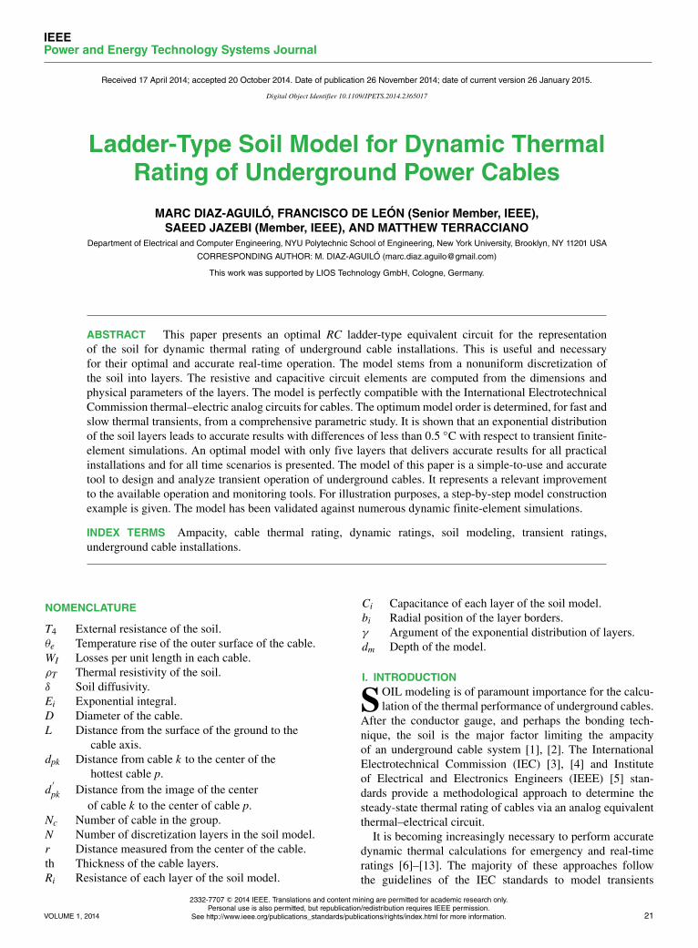
FIGURE 1. Equivalent electrothermal circuit (T equivalent circuit)used for each of the individual layers modeled in this paper.

into several concentric layers. Each soil layer is representedwith its RC thermal T equivalent circuit (Fig. 1) to becompatible with the IEC standards [2], [3]. The soil modelparameters are computed from the thermal resistivity, the heatcapacity of the soil, and the dimensions of each layer using thefollowing formula, which are applicable to hollow cylindricalshapes [2]:

R =ρ

2πlog

(1+

thrint

)(8)

C = π(r2ext − r

2int)· Cp (9)

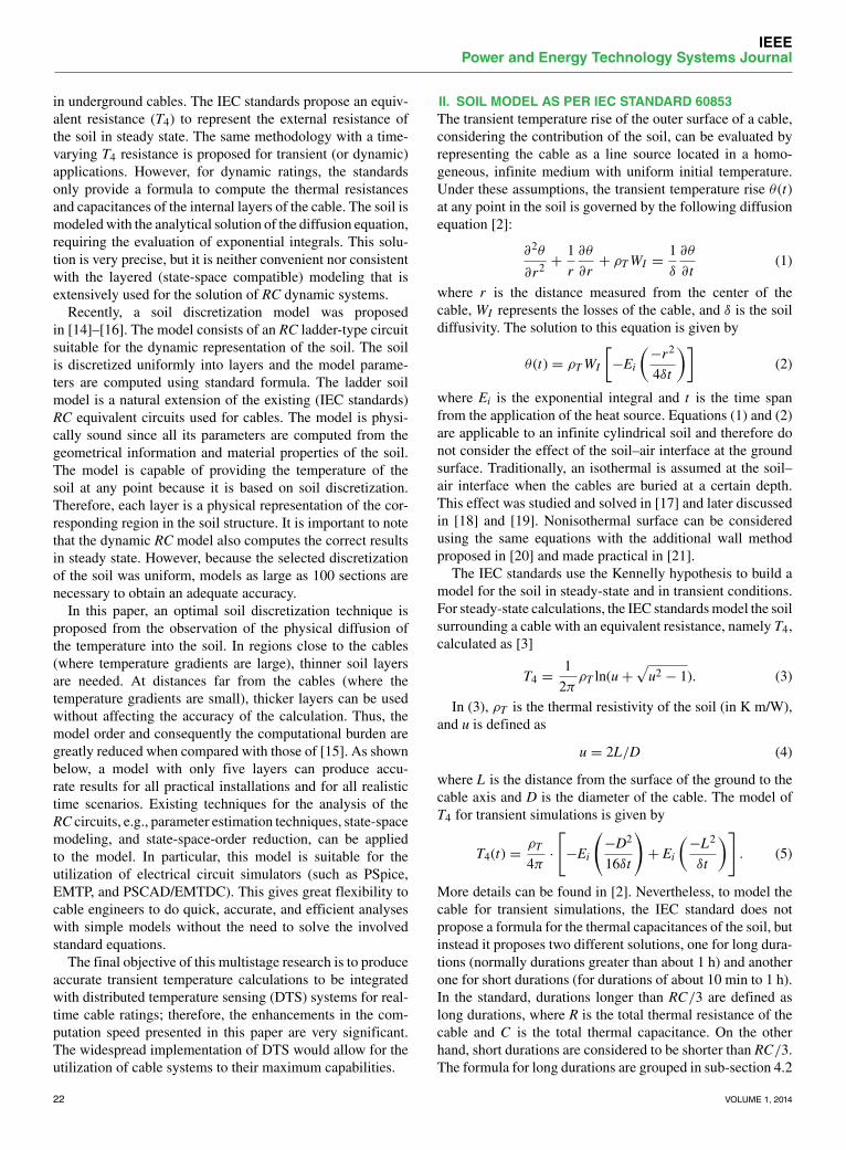
where ρ is the thermal resistivity of the layer under study, th isthe thickness, rext and rint stand for the layer external radiusand internal radius, respectively, andCp is the heat capacity ofthe material. This formulation is consistent with the one usedin the IEC standards [3], [4], and in [15]. However, note thatin this paper, R is used as the symbol for thermal resistanceswhere the IEC standards use T. Each layer is represented witha T equivalent circuit, as shown in Fig. 1.The physical discretization of the soil can be observed in

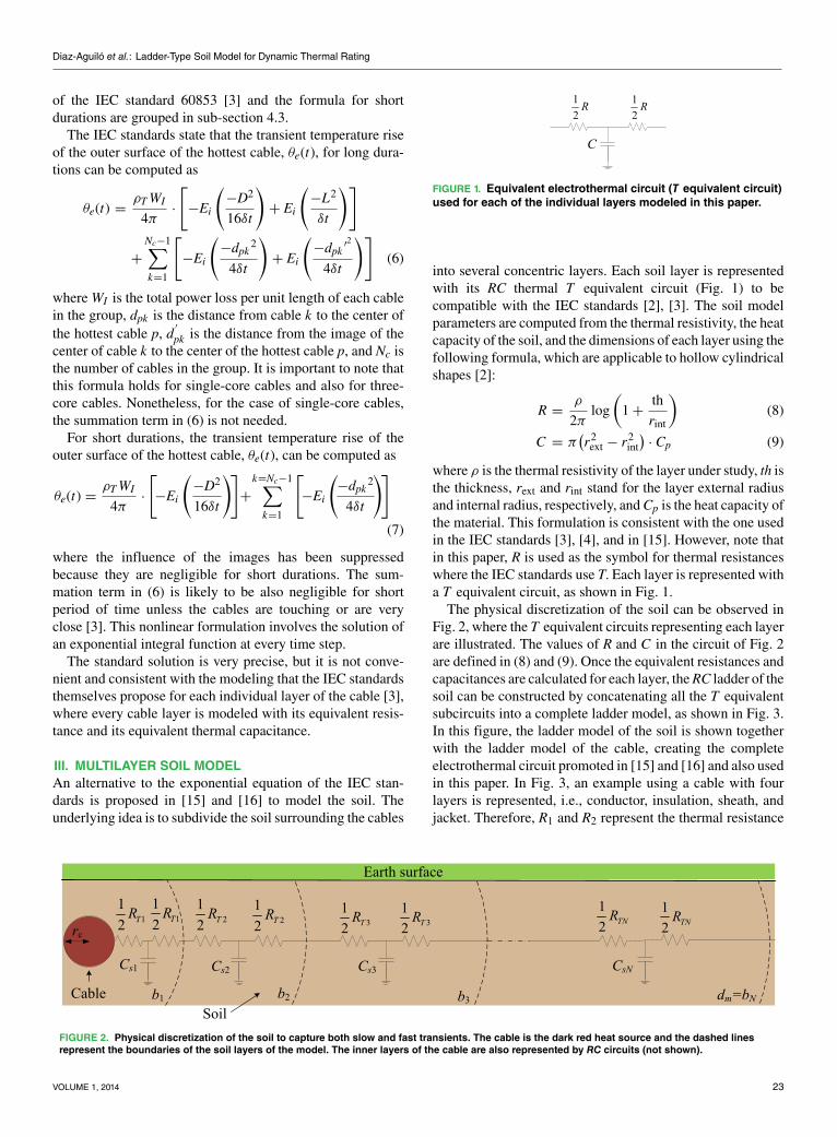
Fig. 2, where the T equivalent circuits representing each layerare illustrated. The values of R and C in the circuit of Fig. 2are defined in (8) and (9). Once the equivalent resistances andcapacitances are calculated for each layer, theRC ladder of thesoil can be constructed by concatenating all the T equivalentsubcircuits into a complete ladder model, as shown in Fig. 3.In this figure, the ladder model of the soil is shown togetherwith the ladder model of the cable, creating the completeelectrothermal circuit promoted in [15] and [16] and also usedin this paper. In Fig. 3, an example using a cable with fourlayers is represented, i.e., conductor, insulation, sheath, andjacket. Therefore, R1 and R2 represent the thermal resistance

FIGURE 2. Physical discretization of the soil to capture both slow and fast transients. The cable is the dark red heat source and the dashed linesrepresent the boundaries of the soil layers of the model. The inner layers of the cable are also represented by RC circuits (not shown).

VOLUME 1, 2014 23


FIGURE 3. Complete ladder-type equivalent circuit for the cable and its surrounding soil.

of the insulation, R3 and R4 represent the resistance of thejacket, while C1,C2,C3, and C4 correspond to the thermalcapacitances of the conductor, insulation, sheath, and jacket,respectively. Heat sourcesQ1,Q2, andQ3 represent the lossesin the conductor, insulation, and sheath, respectively.

The computation of the thermal resistances is givenin (8). The thermal capacitances can be computed using (9).The method to compute losses is described in [4], whichincludes temperature, frequency, and voltage dependencies.Parameters Rsi and Csi represent the thermal resistances andcapacitances of the soil subdivisions and Tamb is the datumambient temperature. The relationships between the resis-tances shown in Figs. 2 and 3 are the following:

Rs0 =12RT1 (10a)

Rsi =12(RTi + RTi+1) for i = 1, 2, . . . ,N − 1 (10b)

RsN =12RTN. (10c)

To obtain an accurate dynamic representation of the ther-mal transients, a multilayer model of the soil is needed. Thisis so to physically represent the diffusion of heat in the soil.When current circulates in a conductor, the temperature of thesoil layers close to (or touching) the cable increases quickly.Therefore, an RC circuit with a small time constant should beused to represent the fast transients. The heat takes (much)longer to reach the soil layers that are far from the cable.Then, an RC circuit with a large time constant is adequateto represent the long time necessary for the heat to reach farsoil layers. Since fast transients have smaller time constants,narrower soil subdivisions are needed for the soil close to thecable. In contrast, the soil layers that are further apart fromthe cable play a major role in the slow transients with largertime constants. Therefore, they can be discretized in thickerlayers. This attribute is not considered in themodels presentedin [15] and [16]. Nonetheless, this feature is the key to obtain-ing a model with only a few sections with the same accuracyas a large order model, but with reduced computation time.Thus, the reduced-order model is suitable for real-time calcu-lations. Fig. 2 shows how the size of the subdivision increasesas one moves away from the cable.

A. DISTRIBUTION OF LAYERSIn this section, a discretization approach is proposed for thesubdivision of soil into layers. As discussed above, numerous

and thin layers are preferable near the cable and thicker layersare sufficient in the far region of the soil. Since the analyticalsolution of the heat diffusion problem is an exponential inte-gral (5), an exponential discretization of the soil is proposedas follows:

bi = rc + (dm − rc) ·eγ ·i − 1eγ ·N − 1

(11)

where bi are the radial positions of the layer borders, rcis the radius of the cable, N is the number of layersof the discretization, and dm is the depth of the model.Finally, i = 0, 1, . . . ,N represents the index of the layer.Therefore, there are N + 1 boundaries that correspond toN layers in the soil model. γ is the argument of the expo-nential distribution and it has to be a positive number. Smallvalues of γ represent quasi-linear distributions, hence theyimply the same number of layers in the proximity of thecable than in the far soil. This case represents the linearmodel presented in [15] and [16]. The fast transients maynot be captured correctly unless a very large number oflayers is selected (100 sections are used in [15]). On theother hand, large values of γ imply that a single (and thick)layer represents the effects of the far soil. This leads to asituation where the slow transients are not properly captured.Note that the exponential discretization proposed in (11)assumes that the layers of the model must have progressivelyincreasing thicknesses (as shown in Fig. 2). This assumptionis physically sound because the heat flux and temperaturegradient are higher close to the cable, where the model is dis-cretized finer [2]. The optimum value of γ will be computedin Section III-D.

Other two important parameters of the soil model are thedepth of the model dm (i.e., the position of the last layer thatis considered) and the number of layers N . The impact of theaforementioned parameters is investigated in the followingsections.

B. DEPTH OF THE MODELThe depth of the model, dm, is a parameter that dependson the burial depth of the cable. As it has been definedin (11), the value of dm will have an effect in the final thermalresistance representing the external environment of the cable.This resistance is defined as T4 in the IEC standard [3].For single isolated buried cables, the value of T4 iscalculated using (3) and (4). These formulae were first intro-duced in [17], but the final formulation was proposed in [18]

24 VOLUME 1, 2014


and was further developed in [19]. The expressions for T4 areobtained using the method of images and consider the soil–airinterface as an isotherm. These expressions give very accurateresults for steady-state analysis of buried cables. Therefore,to assure that the model of this paper computes the steadystate correctly, the model should have the same total externalresistance as computed by (3). The same assumption is madein the models presented in [15]. Therefore, (3) should beequated to the sum of the resistances of all layers given in (8),yielding

T4 =N−1∑i=0

ρT

2πlog

(1+

bi+1 − bibi

). (12)

For the case when N = 1, a simple algebraic manipulation of(12) leads to

dm = L +√L2 − r2c . (13)

Note also that due to the properties of logarithms (12) can berewritten as

T4 =ρT

2πlog

(N−1∏i=0

bi+1bi

)=ρT

2πlog

(bNb0

)(14)

and the value of (14) is equivalent to a model with one singlelayer. Therefore, the result obtained in (13) is valid for any N .To support the validity of the formula and to corroborate the

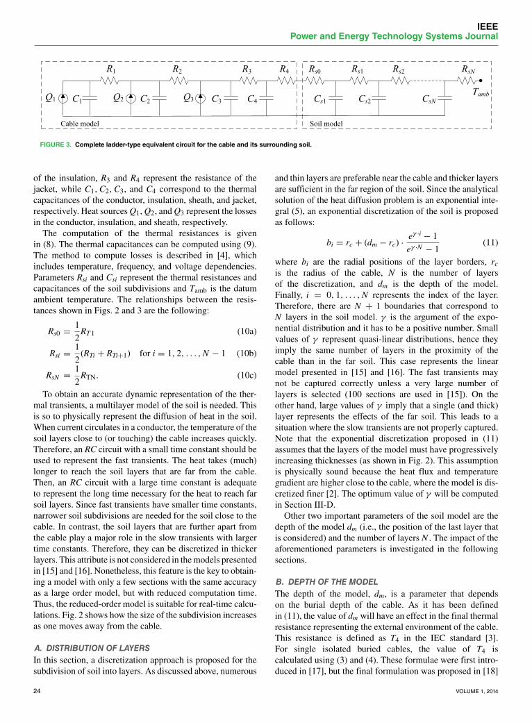
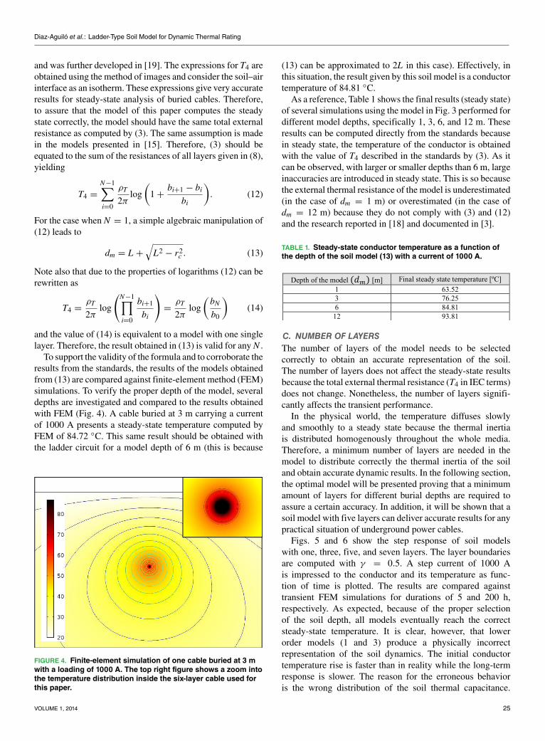
results from the standards, the results of the models obtainedfrom (13) are compared against finite-element method (FEM)simulations. To verify the proper depth of the model, severaldepths are investigated and compared to the results obtainedwith FEM (Fig. 4). A cable buried at 3 m carrying a currentof 1000 A presents a steady-state temperature computed byFEM of 84.72 ◦C. This same result should be obtained withthe ladder circuit for a model depth of 6 m (this is because

FIGURE 4. Finite-element simulation of one cable buried at 3 mwith a loading of 1000 A. The top right figure shows a zoom intothe temperature distribution inside the six-layer cable used forthis paper.

(13) can be approximated to 2L in this case). Effectively, inthis situation, the result given by this soil model is a conductortemperature of 84.81 ◦C.As a reference, Table 1 shows the final results (steady state)

of several simulations using the model in Fig. 3 performed fordifferent model depths, specifically 1, 3, 6, and 12 m. Theseresults can be computed directly from the standards becausein steady state, the temperature of the conductor is obtainedwith the value of T4 described in the standards by (3). As itcan be observed, with larger or smaller depths than 6 m, largeinaccuracies are introduced in steady state. This is so becausethe external thermal resistance of the model is underestimated(in the case of dm = 1 m) or overestimated (in the case ofdm = 12 m) because they do not comply with (3) and (12)and the research reported in [18] and documented in [3].

TABLE 1. Steady-state conductor temperature as a function ofthe depth of the soil model (13) with a current of 1000 A.

C. NUMBER OF LAYERSThe number of layers of the model needs to be selectedcorrectly to obtain an accurate representation of the soil.The number of layers does not affect the steady-state resultsbecause the total external thermal resistance (T4 in IEC terms)does not change. Nonetheless, the number of layers signifi-cantly affects the transient performance.In the physical world, the temperature diffuses slowly

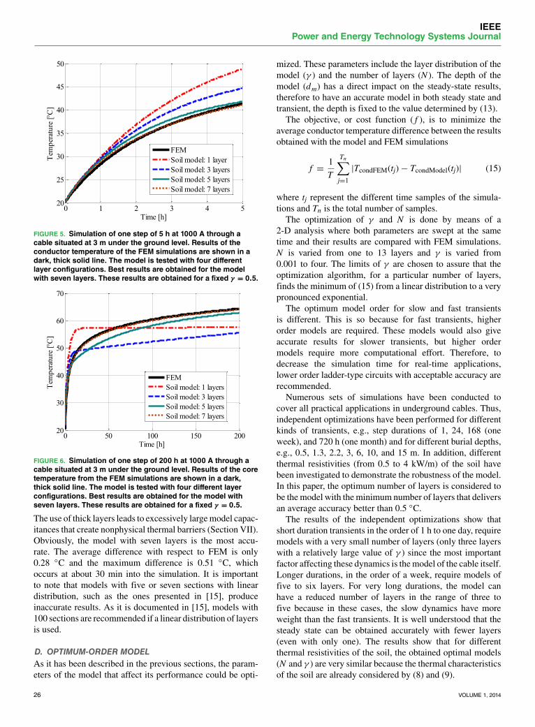
and smoothly to a steady state because the thermal inertiais distributed homogenously throughout the whole media.Therefore, a minimum number of layers are needed in themodel to distribute correctly the thermal inertia of the soiland obtain accurate dynamic results. In the following section,the optimal model will be presented proving that a minimumamount of layers for different burial depths are required toassure a certain accuracy. In addition, it will be shown that asoil model with five layers can deliver accurate results for anypractical situation of underground power cables.Figs. 5 and 6 show the step response of soil models

with one, three, five, and seven layers. The layer boundariesare computed with γ = 0.5. A step current of 1000 Ais impressed to the conductor and its temperature as func-tion of time is plotted. The results are compared againsttransient FEM simulations for durations of 5 and 200 h,respectively. As expected, because of the proper selectionof the soil depth, all models eventually reach the correctsteady-state temperature. It is clear, however, that lowerorder models (1 and 3) produce a physically incorrectrepresentation of the soil dynamics. The initial conductortemperature rise is faster than in reality while the long-termresponse is slower. The reason for the erroneous behavioris the wrong distribution of the soil thermal capacitance.

VOLUME 1, 2014 25


FIGURE 5. Simulation of one step of 5 h at 1000 A through acable situated at 3 m under the ground level. Results of theconductor temperature of the FEM simulations are shown in adark, thick solid line. The model is tested with four differentlayer configurations. Best results are obtained for the modelwith seven layers. These results are obtained for a fixed γ = 0.5.

FIGURE 6. Simulation of one step of 200 h at 1000 A through acable situated at 3 m under the ground level. Results of the coretemperature from the FEM simulations are shown in a dark,thick solid line. The model is tested with four different layerconfigurations. Best results are obtained for the model withseven layers. These results are obtained for a fixed γ = 0.5.

The use of thick layers leads to excessively largemodel capac-itances that create nonphysical thermal barriers (Section VII).Obviously, the model with seven layers is the most accu-rate. The average difference with respect to FEM is only0.28 ◦C and the maximum difference is 0.51 ◦C, whichoccurs at about 30 min into the simulation. It is importantto note that models with five or seven sections with lineardistribution, such as the ones presented in [15], produceinaccurate results. As it is documented in [15], models with100 sections are recommended if a linear distribution of layersis used.

D. OPTIMUM-ORDER MODELAs it has been described in the previous sections, the param-eters of the model that affect its performance could be opti-

mized. These parameters include the layer distribution of themodel (γ ) and the number of layers (N ). The depth of themodel (dm) has a direct impact on the steady-state results,therefore to have an accurate model in both steady state andtransient, the depth is fixed to the value determined by (13).The objective, or cost function ( f ), is to minimize the

average conductor temperature difference between the resultsobtained with the model and FEM simulations

f =1T

Tn∑j=1

|TcondFEM(tj)− TcondModel(tj)| (15)

where tj represent the different time samples of the simula-tions and Tn is the total number of samples.The optimization of γ and N is done by means of a

2-D analysis where both parameters are swept at the sametime and their results are compared with FEM simulations.N is varied from one to 13 layers and γ is varied from0.001 to four. The limits of γ are chosen to assure that theoptimization algorithm, for a particular number of layers,finds the minimum of (15) from a linear distribution to a verypronounced exponential.The optimum model order for slow and fast transients

is different. This is so because for fast transients, higherorder models are required. These models would also giveaccurate results for slower transients, but higher ordermodels require more computational effort. Therefore, todecrease the simulation time for real-time applications,lower order ladder-type circuits with acceptable accuracy arerecommended.Numerous sets of simulations have been conducted to

cover all practical applications in underground cables. Thus,independent optimizations have been performed for differentkinds of transients, e.g., step durations of 1, 24, 168 (oneweek), and 720 h (one month) and for different burial depths,e.g., 0.5, 1.3, 2.2, 3, 6, 10, and 15 m. In addition, differentthermal resistivities (from 0.5 to 4 kW/m) of the soil havebeen investigated to demonstrate the robustness of the model.In this paper, the optimum number of layers is considered tobe themodel with theminimum number of layers that deliversan average accuracy better than 0.5 ◦C.The results of the independent optimizations show that

short duration transients in the order of 1 h to one day, requiremodels with a very small number of layers (only three layerswith a relatively large value of γ ) since the most importantfactor affecting these dynamics is themodel of the cable itself.Longer durations, in the order of a week, require models offive to six layers. For very long durations, the model canhave a reduced number of layers in the range of three tofive because in these cases, the slow dynamics have moreweight than the fast transients. It is well understood that thesteady state can be obtained accurately with fewer layers(even with only one). The results show that for differentthermal resistivities of the soil, the obtained optimal models(N and γ ) are very similar because the thermal characteristicsof the soil are already considered by (8) and (9).

26 VOLUME 1, 2014


Note that, for a fixed value of γ , a model with more layersalways gives more accurate results. However, the drawback ofa higher order models is the increased computational burden(see Section VII for more details). In addition, for deeplyburied cables, the amount of soil in the model is larger; hence,thinner layers close to the cable have to be obtained either byincreasing γ or increasing N . Simulation results show thatfor larger burial depths, a model with the same number oflayers can deliver the necessary accuracy if γ is increased.Nevertheless, when the burial depth increases to large values,such as 10 or 15 m, normally the optimum model requiresmore layers.

Extensive independent studies show that for practicalinstallations (burial depths lower than 15 m, simulation timesbetween 1 h and one month, and thermal resistivities rangingfrom 0.5 to 4 Km/W), the necessary number of layers in themodel is always between three and six while guaranteeingaccuracies better than 0.5 ◦C.Table 2 shows the optimal models for all time scenar-

ios described above with independent optimization for eachburial depth. One can conclude that for larger burial depths,more layers are required.

TABLE 2. Optimum number of layers and optimum value ofgamma of the soil model for different burial depths.

In addition to the independent optimizations, to find ageneral and versatile model that delivers accurate results inmany different time scenarios and for different installations,a collective optimization has been conducted. This optimiza-tion finds the model that best performs in average for allthe time scenarios, burial depths, and thermal resistivitiesdescribed above. The results of this optimization show thatthe general model has five layers with γ = 1.32. The generalmodel performs with an average accuracy of 0.44 ◦C acrossall scenarios.

IV. NUMERICAL EXAMPLEIn this section, a numerical example is given to calculatethe optimal (general) model found in the previous section.The model calculated here has five layers and γ = 1.32.The radius of the cable for this example is rc = 0.053 mand the burial depth is L = 1 m. Then, using (13) one cancalculate dm = 1.999 m. The next step is the calculation ofthe boundary positions of the soil discretization using (11).The results are listed in the first row of Table 3. Then, thecorresponding thickness and the interior and exterior radiusof every layer can be calculated, which are listed in rows

TABLE 3. Values of thermal resistances and capacitances for theoptimal soil model found in Section IV.

two, three, and four of the same table. Next, using (8) and (9)together with a soil resistivity of ρ = 1 K m/W and a Cp =1.44 · 106 J/(K m3), the values of RTi and Csi correspondingto the model of Fig. 2 are calculated. Finally, with (10), thevalues for Rsi are obtained. The parameter values of the model(Fig. 3) are given in rows five and six of Table 3.

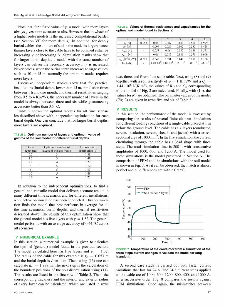
V. RESULTSIn this section, the performance of the model is assessed bycomparing the results of several finite-element simulationsfor different loading conditions of a single cable placed at 1 mbelow the ground level. The cable has six layers (conductor,screen, insulation, screen, sheath, and jacket) with a cross-sectional area of 1000mm2. In the first simulation, the currentcirculating through the cable has a load shape with threesteps. The total simulation time is 200 h with consecutiveamplitudes of 1000, 600, and 1200 A. The model used forthese simulations is the model presented in Section V. Thecomparison of FEM and the simulations with the soil modelis shown in Fig. 7. As it can be observed, the match is almostperfect and all differences are within 0.5 ◦C.

FIGURE 7. Temperature of the conductor from a simulation of thethree steps current changes to validate the model for longtransient.

A second case study is carried out with faster currentvariations that last for 24 h. The 24-h current steps appliedto the cable are of 1000, 600, 1200, 800, 400, and 1000 A,in a successive order. Fig. 8 compares the results againstFEM simulations. Once again, the mismatches between

VOLUME 1, 2014 27


FEM and the general model results are minimal.

FIGURE 8. Temperature of the conductor from a simulation of the24-h steps current changes to validate the model in one daytransients situations.

FIGURE 9. Temperature of the conductor from a simulation of the1-h steps current changes to validate the model for the shorttransients. Note the poor performance of the model with onesingle layer in comparison with the general model with fivelayers.

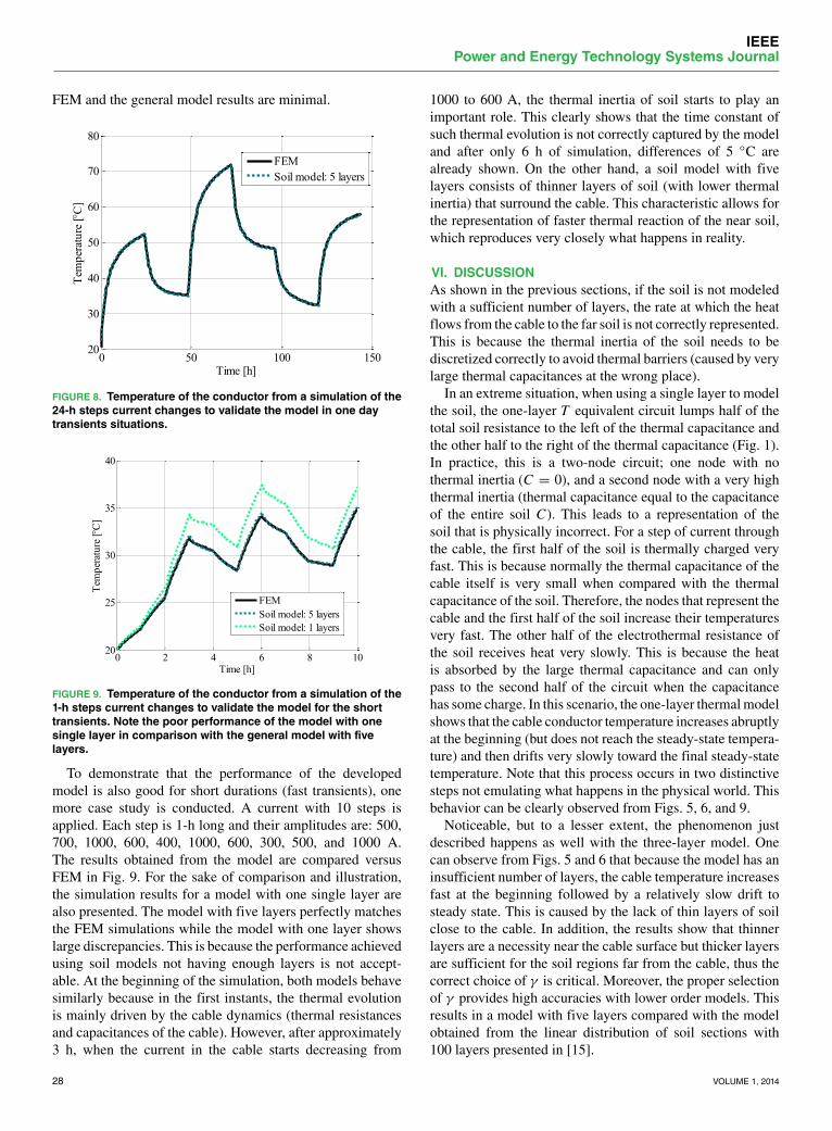
To demonstrate that the performance of the developedmodel is also good for short durations (fast transients), onemore case study is conducted. A current with 10 steps isapplied. Each step is 1-h long and their amplitudes are: 500,700, 1000, 600, 400, 1000, 600, 300, 500, and 1000 A.The results obtained from the model are compared versusFEM in Fig. 9. For the sake of comparison and illustration,the simulation results for a model with one single layer arealso presented. The model with five layers perfectly matchesthe FEM simulations while the model with one layer showslarge discrepancies. This is because the performance achievedusing soil models not having enough layers is not accept-able. At the beginning of the simulation, both models behavesimilarly because in the first instants, the thermal evolutionis mainly driven by the cable dynamics (thermal resistancesand capacitances of the cable). However, after approximately3 h, when the current in the cable starts decreasing from

1000 to 600 A, the thermal inertia of soil starts to play animportant role. This clearly shows that the time constant ofsuch thermal evolution is not correctly captured by the modeland after only 6 h of simulation, differences of 5 ◦C arealready shown. On the other hand, a soil model with fivelayers consists of thinner layers of soil (with lower thermalinertia) that surround the cable. This characteristic allows forthe representation of faster thermal reaction of the near soil,which reproduces very closely what happens in reality.

VI. DISCUSSIONAs shown in the previous sections, if the soil is not modeledwith a sufficient number of layers, the rate at which the heatflows from the cable to the far soil is not correctly represented.This is because the thermal inertia of the soil needs to bediscretized correctly to avoid thermal barriers (caused by verylarge thermal capacitances at the wrong place).In an extreme situation, when using a single layer to model

the soil, the one-layer T equivalent circuit lumps half of thetotal soil resistance to the left of the thermal capacitance andthe other half to the right of the thermal capacitance (Fig. 1).In practice, this is a two-node circuit; one node with nothermal inertia (C = 0), and a second node with a very highthermal inertia (thermal capacitance equal to the capacitanceof the entire soil C). This leads to a representation of thesoil that is physically incorrect. For a step of current throughthe cable, the first half of the soil is thermally charged veryfast. This is because normally the thermal capacitance of thecable itself is very small when compared with the thermalcapacitance of the soil. Therefore, the nodes that represent thecable and the first half of the soil increase their temperaturesvery fast. The other half of the electrothermal resistance ofthe soil receives heat very slowly. This is because the heatis absorbed by the large thermal capacitance and can onlypass to the second half of the circuit when the capacitancehas some charge. In this scenario, the one-layer thermalmodelshows that the cable conductor temperature increases abruptlyat the beginning (but does not reach the steady-state tempera-ture) and then drifts very slowly toward the final steady-statetemperature. Note that this process occurs in two distinctivesteps not emulating what happens in the physical world. Thisbehavior can be clearly observed from Figs. 5, 6, and 9.Noticeable, but to a lesser extent, the phenomenon just

described happens as well with the three-layer model. Onecan observe from Figs. 5 and 6 that because the model has aninsufficient number of layers, the cable temperature increasesfast at the beginning followed by a relatively slow drift tosteady state. This is caused by the lack of thin layers of soilclose to the cable. In addition, the results show that thinnerlayers are a necessity near the cable surface but thicker layersare sufficient for the soil regions far from the cable, thus thecorrect choice of γ is critical. Moreover, the proper selectionof γ provides high accuracies with lower order models. Thisresults in a model with five layers compared with the modelobtained from the linear distribution of soil sections with100 layers presented in [15].

28 VOLUME 1, 2014


The lower order model is easier and simpler for engi-neers to implement in graphical software such as PSPICEor EMTP. It also reduces considerably the amount of timethat is needed by the engine to solve the thermal problem.To assess the impact of the model size in computation speed,comparative speed tests have been conducted. Table 4 showsthe computation time to solve the thermal problem with a soilmodel of five layers, compared with soil models of 50 and100 layers. The results are shown for two different scenarios:1) using a solver engine that uses efficient matrix multiplica-tion libraries such as MATLAB or Lapack; and 2) simplersoftware such as standard C code. One can see that in thefirst scenario, the computation speed for a five-layer modelis 3.5 times faster than for a 100-layer model, and in thesecond scenario the speed is 20 times faster. Similar resultsare also reported in [15], where an almost 30 times highercomputation time is reported for models with 100 sections.Computation time is a significant factor in the context of real-time prediction systems, thus a model with lower computa-tional burden leads to faster real-time algorithms.

TABLE 4. Computation speed in milliseconds per time step on acomputer with i5 CPU at 2.67 MHz with 4 GB of RAM.

VII. CONCLUSIONThis paper has introduced an optimal soil model based ona physical discretization of the soil into a few layers. Themodel consists of a series of lumped T -shaped RC circuitsrepresenting the thermal resistances and capacitances of thesoil layers. The new optimal model provides up to 20 timesfaster response than the currently available approaches. Thefaster behavior is due to the lower order model obtained fromthe nonuniform spatial discretization of the soil. The modelorder has been optimized through a comprehensive paramet-ric analysis of cable installation depth, thermal resistivity,and simulation time. It has been determined that a modelof order five can represent all typical transients on commoninstallations.

A numerical example illustrates how easy it is to obtainthe model. In addition, all the analytical tools available forthe analysis of state-space equations apply to this model.Therefore, the model is ideally suited for applications in thecontext of real-time operations of underground power cables.Such an accurate and fast model will represent a relevantenhancement to the actual real-time monitoring systems forpower distribution and transmission cables, making themmore efficient and more robust.

ACKNOWLEDGMENTThe authors would like to thank G. Álvarez from theRed Eléctrica de España, Madrid, Spain, for useful and

interesting discussions. He was in part the motivation of thispaper.

REFERENCES[1] F. de León, ‘‘Major factors affecting cable ampacity,’’ in Proc. IEEE Power

Eng. Soc. Gen. Meet., 2006.[2] G. J. Anders, Rating of Electric Power Cables. New York, NY, USA:

McGraw-Hill, 1997.[3] Calculation of the Cyclic and Emergency Rating of Cables,

IEC Standards 60853-1 and IEC 60853-2, 1989.[4] Calculation of the Current Ratings, IEC Standards 60287-1 and

IEC 60287-2, 2001.[5] IEEE Standard Power Cable Ampacity Tables, IEEE Standard 835-1994,

1994.[6] M. Matus et al., ‘‘Identification of critical spans for monitoring systems

in dynamic thermal rating,’’ IEEE Trans. Power Del., vol. 27, no. 2,pp. 1002–1009, Apr. 2012.

[7] S.-H. Huang, W.-J. Lee, and M.-T. Kuo, ‘‘An online dynamic cable ratingsystem for an industrial power plant in the restructured electric market,’’IEEE Trans. Ind. Appl., vol. 43, no. 6, pp. 1449–1458, Nov./Dec. 2007.

[8] G. J. Anders, A. Napieralski, M. Zubert, and M. Orlikowski, ‘‘Advancedmodeling techniques for dynamic feeder rating systems,’’ IEEE Trans. Ind.Appl., vol. 39, no. 3, pp. 619–626, May/Jun. 2003.

[9] S. P. Walldorf, J. S. Engelhardt, and F. J. Hoppe, ‘‘The use of real-time monitoring and dynamic ratings for power delivery systems and theimplications for dielectric materials,’’ IEEE Elect. Insul. Mag., vol. 15,no. 5, pp. 28–33, Sep./Oct. 1999.

[10] T. H. Dubaniewicz, P. G. Kovalchik, L. W. Scott, and M. A. Fuller, ‘‘Dis-tributed measurement of conductor temperatures in mine trailing cablesusing fiber-optic technology,’’ IEEE Trans. Ind. Appl., vol. 34, no. 2,pp. 395–398, Mar./Apr. 1998.

[11] D. A. Douglass, A. Edris, and G. A. Pritchard, ‘‘Field application of adynamic thermal circuit rating method,’’ IEEE Trans. Power Del., vol. 12,no. 2, pp. 823–831, Apr. 1997.

[12] D. A. Douglass and A. Edris, ‘‘Real-time monitoring and dynamic thermalrating of power transmission circuits,’’ IEEE Trans. Power Del., vol. 11,no. 3, pp. 1407–1418, Jul. 1996.

[13] G. Z. Ben-Yaacov and J. G. Bohn, ‘‘Methodology for real-time cal-culation of temperature rise and dynamic ratings for distribution sys-tem duct banks,’’ IEEE Trans. Power App. Syst., vol. PAS-101, no. 12,pp. 4604–4610, Dec. 1982.

[14] R. S. Olsen, ‘‘Dynamic loadability of cable based transmissiongrids,’’ Ph.D. dissertation, Dept. Elect. Eng., Tech. Univ. Denmark,Kongens Lyngby, Denmark, 2013.

[15] R. S. Olsen, J. Holboll, and U. S. Gudmundsdottir, ‘‘Dynamic temperatureestimation and real time emergency rating of transmission cables,’’ in Proc.IEEE Power Energy Soc. Gen. Meet., Jul. 2012, pp. 1–8.

[16] R. Olsen, G. J. Anders, J. Holboell, and U. S. Gudmundsdottir, ‘‘Modellingof dynamic transmission cable temperature considering soil-specific heat,thermal resistivity, and precipitation,’’ IEEE Trans. Power Del., vol. 28,no. 3, pp. 1909–1917, Jul. 2013.

[17] A. E. Kennelly, ‘‘Discussion of electrical congress programme,’’ Trans.Amer. Inst. Elect. Eng., vol. 10, pp. 363–369, Jan. 1893.

[18] J. H. Neher, ‘‘The temperature rise of buried cables and pipes,’’ Trans.Amer. Inst. Elect. Eng., vol. 68, no. 1, pp. 9–21, Jul. 1949.

[19] J. H. Neher and M. H. Mcgrath, ‘‘The calculation of the temperature riseand load capability of cable systems,’’ Trans. Amer. Inst. Elect. Eng. PowerApp. Syst. III, vol. 76, no. 3, pp. 752–764, Apr. 1957.

[20] S. S. Kutateladze, Fundamentals of Heat Transfer. New York, NY, USA:Academic, 1963.

[21] S. Purushothaman, F. de León, and M. Terracciano, ‘‘Calculation of cablethermal rating considering non-isothermal earth surface,’’ IET Gener.,Transmiss. Distrib., vol. 8, no. 7, pp. 1354–1361, 2014.

MARC DIAZ-AGUILÓ was born in Barcelona, Spain. He received theM.Sc. degree in telecommunications engineering from the Technical Uni-versity of Catalonia (UPC), Barcelona, Spain, in 2006, the M.Sc. degreein aerospace controls engineering from a joint program between the Insti-tut Supérieur de l’Aéronautique et de l’Espace, Toulouse, France, and theMassachusetts Institute of Technology, Cambridge, MA, USA, in 2008, andthe Ph.D. degree in aerospace simulation and controls from UPC, in 2011.

VOLUME 1, 2014 29


He is currently a Post-Doctoral Researcher with the NYU PolytechnicSchool of Engineering, New York University, Brooklyn, NY, USA. Hiscurrent research interests include power systems, controls, smart-grid imple-mentations, and large systems modeling and simulation.

FRANCISCO DE LEÓN (S’86–M’92–SM’02) received the B.Sc. andM.Sc. (Hons.) degrees from the National Polytechnic Institute, Mexico City,Mexico, in 1983 and 1986, respectively, and the Ph.D. degree from the Uni-versity of Toronto, Toronto, ON, Canada, in 1992, in electrical engineering.

He has held several academic positions in Mexico and has worked forthe Canadian electric industry. Since 2007, he has been an Associate Pro-fessor with the Department of Electrical and Computer Engineering, NYUPolytechnic School of Engineering, New York University, Brooklyn, NY,USA. His current research interests include the analysis of power phenom-ena under nonsinusoidal conditions, transient and steady-state analyses ofpower systems, thermal rating of cables and transformers, and calculation ofelectromagnetic fields applied to machine design and modeling.

Dr. de León is an Editor of the IEEE TRANSACTIONS ON POWER DELIVERY

and the IEEE POWER ENGINEERING LETTERS.

SAEED JAZEBI (S’10–M’14) was born in Kerman, Iran, in 1983. Hereceived the B.Sc. and M.Sc. degrees from Shahid Bahonar University,Kerman, Iran, and the Amirkabir University of Technology, Tehran, Iran, in2006 and 2008, respectively, and the Ph.D. degree from the NYUPolytechnicSchool of Engineering, New York University, Brooklyn, NY, USA, in 2014,all in electrical engineering, where he continues his research as a Post-Doctoral Fellow.

His current research interests include electromagnetic design, modeling,and simulation of electrical machines and power system components, sta-tistical pattern recognition applications in power engineering, power systemprotection, and power quality.

MATTHEW TERRACCIANO received the B.Sc. and M.Sc. degrees inelectrical engineering from the NYU Polytechnic School of Engineering,New York University, Brooklyn, NY, USA, in 2010 and 2012, respectively.

His current research interests include cable ampacity and thermal analysis.

30 VOLUME 1, 2014

ladder-type soil model for dynamic thermal rating of

Documents