laboratory soil tests - الجامعة...
TRANSCRIPT
LABORATORY SOIL
TESTS
University of Technology
Building & Const. Eng. Dept.
Highway & Bridges Branch
Supervised by
Dr. Mahmood Rasheed Lec. Kawther Yaly Hussain
2014
CONTENTS page No.
1. Specific gravity of soil solids.
2. Sieve analysis.
3. Hydrometer analysis.
4. Field density by sand replacement method.
5. Field density by rubber balloon method.
6. Liquid and plastic limit of soil.
7. Shrinkage limit.
8. Standard proctor test.
9. Constant head permeability test.
10. Variable head permeability test.
11. Consolidation test.
12. Direct shear test.
13. Unconfined compression test.
14. Vane shear test.
15. Unconsolidated undrained test
16. Consolidated drained test
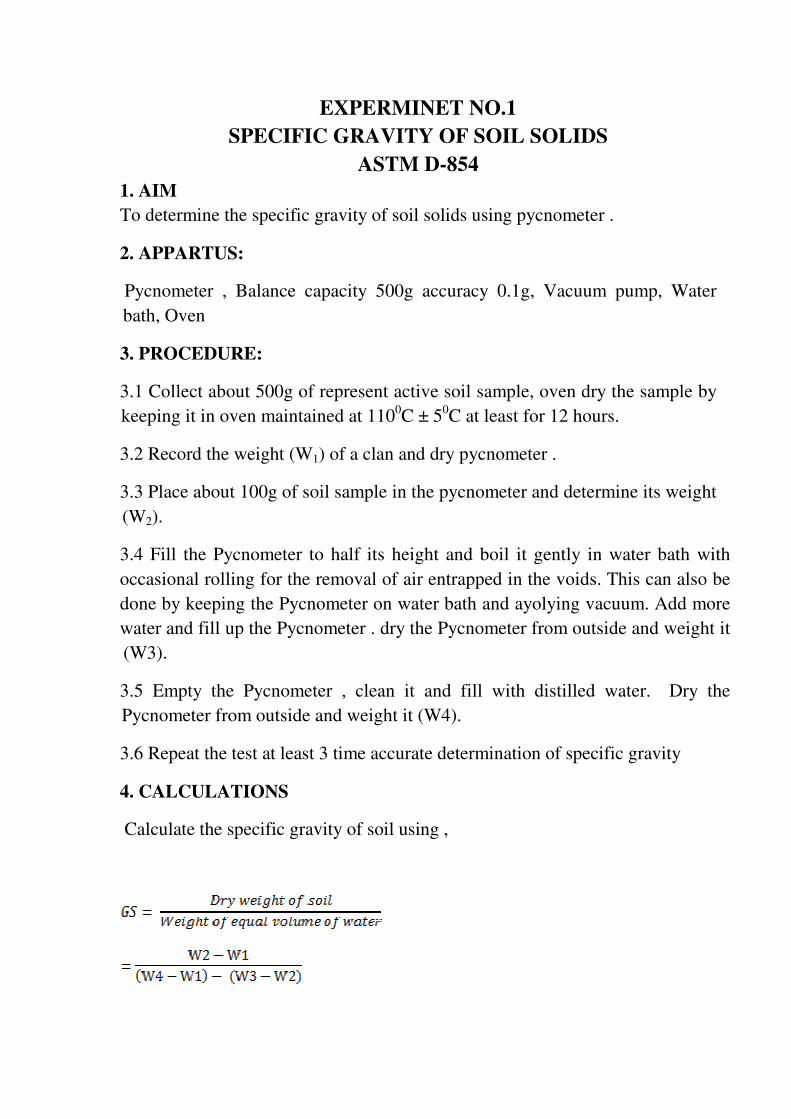
EXPERMINET NO.1
SPECIFIC GRAVITY OF SOIL SOLIDS
ASTM D-854
1. AIM
To determine the specific gravity of soil solids using pycnometer .
2. APPARTUS:
Pycnometer , Balance capacity 500g accuracy 0.1g, Vacuum pump, Water
bath, Oven
3. PROCEDURE:
3.1 Collect about 500g of represent active soil sample, oven dry the sample by
keeping it in oven maintained at 1100C ± 5
0C at least for 12 hours.
3.2 Record the weight (W1) of a clan and dry pycnometer .
3.3 Place about 100g of soil sample in the pycnometer and determine its weight
(W2).
3.4 Fill the Pycnometer to half its height and boil it gently in water bath with
occasional rolling for the removal of air entrapped in the voids. This can also be
done by keeping the Pycnometer on water bath and ayolying vacuum. Add more
water and fill up the Pycnometer . dry the Pycnometer from outside and weight it
(W3).
3.5 Empty the Pycnometer , clean it and fill with distilled water. Dry the
Pycnometer from outside and weight it (W4).
3.6 Repeat the test at least 3 time accurate determination of specific gravity
4. CALCULATIONS
Calculate the specific gravity of soil using ,

5. RESULTS
Fond the average specific gravity of soil sample.
6. DATA SHEET
Trial Trial Trial Details Sr.
3 2 1 No.
Pycnometer No. 1
Wt. of empty Pycnometer W1 2
Wt. of Pycnometer + dry soil W2 3
Wt. of Pycnometer + dry soil + water W3 4
Wt. of Pycnometer + water W4 5
Specific gravity of soil GS 6
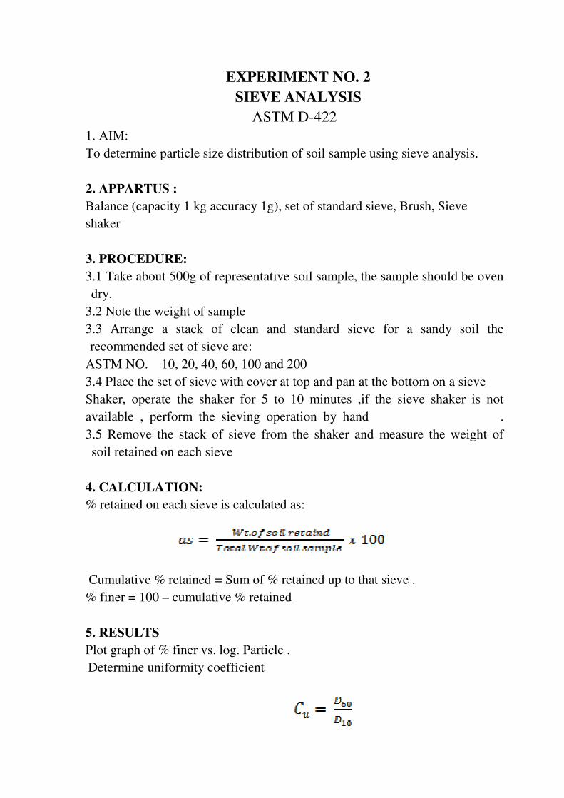
EXPERIMENT NO. 2
SIEVE ANALYSIS
ASTM D-422
1. AIM:
To determine particle size distribution of soil sample using sieve analysis.
2. APPARTUS :
Balance (capacity 1 kg accuracy 1g), set of standard sieve, Brush, Sieve
shaker
3. PROCEDURE:
3.1 Take about 500g of representative soil sample, the sample should be oven
dry.
3.2 Note the weight of sample
3.3 Arrange a stack of clean and standard sieve for a sandy soil the
recommended set of sieve are:
ASTM NO. 10, 20, 40, 60, 100 and 200
3.4 Place the set of sieve with cover at top and pan at the bottom on a sieve
Shaker, operate the shaker for 5 to 10 minutes ,if the sieve shaker is not
available , perform the sieving operation by hand .
3.5 Remove the stack of sieve from the shaker and measure the weight of
soil retained on each sieve
4. CALCULATION:
% retained on each sieve is calculated as:
Cumulative % retained = Sum of % retained up to that sieve .
% finer = 100 – cumulative % retained
5. RESULTS
Plot graph of % finer vs. log. Particle .
Determine uniformity coefficient
And coefficient of curvature
6. CHECKLIST:
1. For hand sieving change the mode of shaking so that grains are
continuously moved on the screen of sieve .
2. If the recommended sieve size are not available select the nearest
available size .
3. This analysis is valid for soils having % finer on sieve No. 200 less
than 10 to 12%.
4. Check that the loss in weight of residue is less than 2%.
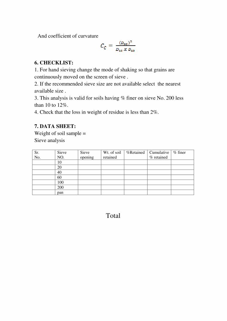
7. DATA SHEET:
Weight of soil sample =
Sieve analysis
% finer Cumulative
% retained
%Retained Wt. of soil
retained
Sieve
opening
Sieve
NO.
Sr.
No.
10
20
40
60
100
200
pan
Total
EXPERIMENT NO. 3
HYDROMETER ANALYSIS
ASTM D-422
1. AIM
To determine grain size distribution of soil, which contains appreciable quantity
of soil passing ASTM 200 sieve ( 0.075 mm).
2. APPARATUS:
Standard hydrometer
Two graduated cylinders ( capacity 1000 cc)
Balance ( capacity 100g accuracy 0.1 g)
Drying oven
High speed stirrer
Thermometer ( range to 50 0c , accuracy 0.1
0c)
Stop watch
ASTM sieve No. 200 (0.075 mm)
3. PROCEDURE:
3.1 Record area of cross section of cylinder A, volume of hydrometer Vh ,
length of the bulb of hydrometer L2, the reading of hydrometer R and the
corresponding length from the top of the bulb , from these observations
calibrate the hydrometer . the readings of hydrometer R varies from – 5to 30 for
a hydrometer calibration from 0.995 to 1.030.
3.2 Record the height of meniscus rise on stem of hydrometer .
3.3 Take about 50g oven dry soil passing through ASTM sieve No. 200 .
3.4 Prepare solution of dispersing agent by adding 40g of sodium
hexametaphosphate to 1000 cc of distilled water.
3.5 Add 125 cc of the solution prepared in 3.4 to the soil sample.
3.6 Transfer the mixture to high speed stirrer and add some more distilled
precaution not to lose any soil .
3.7 Operate the stirrer for 3 to 5 minutes then transfer the mixture from stirrer
cup to graduated cylinder , called as , sedimentation jar. Rinse the cup
thoroughly to transfer all the soil to the sedimentation jar.
3.8 Add some more distilled water to make the volume of suspension equal to
1000 cc .
3.9 Fill a graduated cylinder by 1000 cc of distills water. This cylinder is called
as , control jar.
3.10 Cover the sedimentation jar either by rubber stopped or by palm of hand
and agitate the solution by moving the jar upside down for about 30 sec.
3.11 Insert hydrometer in the sedimentation jar and start the stop watch.
Take the hydrometer readings at total elapsed time of 1/2 , 1 ,2 , and 4 minutes
without removing the hydrometer.
3.12 Repeat the steps 3.10 and 3.11 till the initial reading agree.
3.13 After agreement of initial readings continue to take readings at elapsed
times of 9, 16, 25,36,49,64, and 121 minutes. Afterwards the readings are taken
at elapsed when the reading in the sedimentation jar becomes nearly equal to
that in the control jar . After each reading beyond 2 minutes remove the
hydrometer from suspension and store it in the control jar . before each insertion
of the hydrometer , dry the stem.
3.14 Take the temperature reading in the control jar corresponding hydrometer
reading.
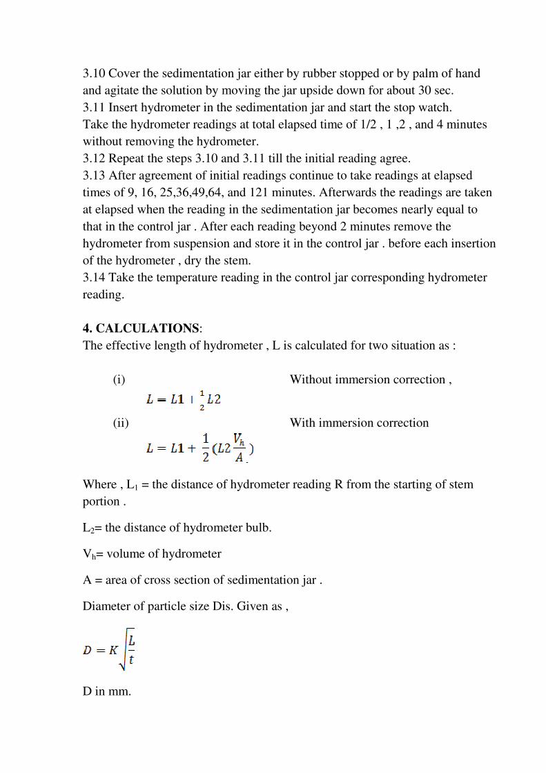
4. CALCULATIONS:
The effective length of hydrometer , L is calculated for two situation as :
(i) Without immersion correction ,
(ii) With immersion correction
Where , L1 = the distance of hydrometer reading R from the starting of stem
portion .
L2= the distance of hydrometer bulb.
Vh= volume of hydrometer
A = area of cross section of sedimentation jar .
Diameter of particle size Dis. Given as ,
D in mm.
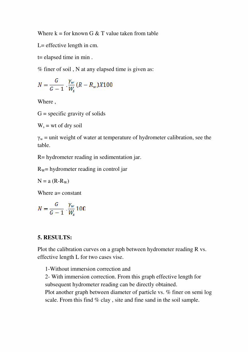
Where k = for known G & T value taken from table
L= effective length in cm.
t= elapsed time in min .
% finer of soil , N at any elapsed time is given as:
Where ,
G = specific gravity of solids
Ws = wt of dry soil
γw = unit weight of water at temperature of hydrometer calibration, see the
table.
R= hydrometer reading in sedimentation jar.
RW= hydrometer reading in control jar
N = a (R-RW)
Where a= constant
5. RESULTS:
Plot the calibration curves on a graph between hydrometer reading R vs.
effective length L for two cases vise.
1-Without immersion correction and
2- With immersion correction. From this graph effective length for
subsequent hydrometer reading can be directly obtained.
Plot another graph between diameter of particle vs. % finer on semi log
scale. From this find % clay , site and fine sand in the soil sample.

6. CHECKLLST
6.1 before each insertion of hydrometer , check that the stem is dry.
6.2 practice insertion of hydrometer and recording of reading before starting
the experiment.
6.3 check that the temperature in sedimentation jar and control jar are same
during the entire period of test .
7. DATA SHEET:
Hydrometer No.
Length of bulb L2=
Volume of hydrometer , Vh=
Area of sedimentation jar , A =
Meniscus correction , cm=
Wt . of dry soil passing ASTM 200 sieve ws=
a- Calibration of hydrometer :
Sr.
hydrometer
No. reading
Hydrometer
reading
corrected for
meniscus
RC=R+Cm
Length
L1
in cm.
Effective
length
Effective length with
immersion correction
1
2
3


EXPERIMENT NO.4
FIELD DENSITY BY SAND
REPLACEMENT METHOD
ASTM D-1556
1. AIM
To determine field density of soil and water content of soil.
2. APPARATUS:
Sand replacement apparatus.
Digging tools
Balance ( capacity 25kg accuracy 10 g)
Balance ( capacity 200g accuracy 0.01g)
uniformly graded medium sand .
3. PROCEDURE
( i ) calibration of equipment :
3.1 Take empty weight of calibration jar , & its size.
3.2 Fill the cylinder of sand replacement apparatus with uniformly graded
medium sand .
3.3 Run the sand from the apparatus to fill the calibration jar. Make the surface
on sand level to the top of jar by straight edge. Record the weight of sand in the
jar.
3.4 Keep the apparatus on flat surface and allow the sand to fill the cone of the
apparatus. Record the weight of sand filled in the cone of the apparatus.
3.5 Find the volume of calibration jar.
3.6 Find the bulk density of sand.
( ii ) field work :
3.7 Take the empty weight of sand replacement apparatus.
3.8 Fill the cylinder of the apparatus with valve closed by calibrated sand and
again take the weight of the apparatus.
3.9 Clean and level the state where field density is desired. Keep the template
with central hole on the leveled ground. Excavate the soil from the hole by
digging tools. Collect all the excavated soil in a tray.
3.10 Keep the sand replacement apparatus with valve in closed position on the
hole of the template.
3.11 Open the valve and allow the sand run down.
3.12 When running of sand stops completely close the valve.
( iii ) laboratory work
3.13 Record the weight of excavated soil
3.14 Record the weight of sand replacement apparatus with left over sand in the
cylinder from this; find the weight of sand used in the field.
3.15 Find the weight of sand used to fill the excavated hole.
3.16 From the bulk density of sand and weight of sand determine the volume of
the excavated soil.
3.17 Take at least two sample of the excavated soil and determine water content
3.18 Determine the field density, water content and dry density of soil
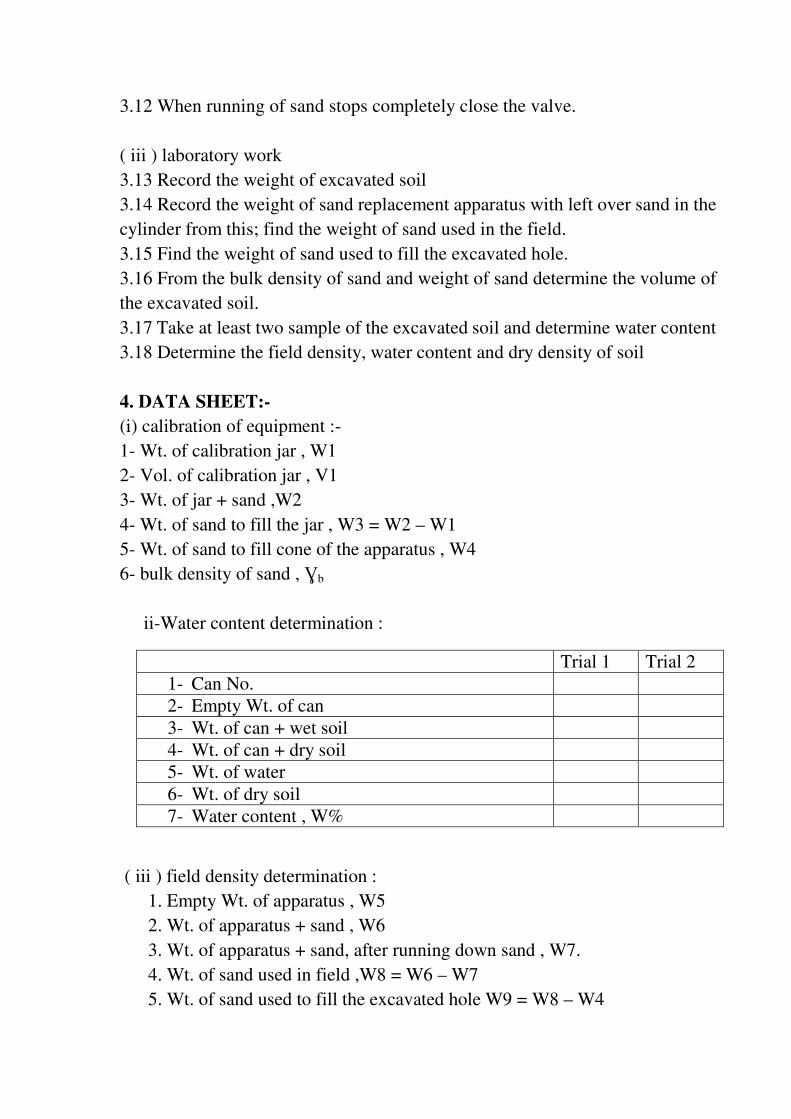
4. DATA SHEET:-
(i) calibration of equipment :-
1- Wt. of calibration jar , W1
2- Vol. of calibration jar , V1
3- Wt. of jar + sand ,W2
4- Wt. of sand to fill the jar , W3 = W2 – W1
5- Wt. of sand to fill cone of the apparatus , W4
6- bulk density of sand , Ɣb
ii-Water content determination :
Trial 1 Trial 2
1- Can No.
2- Empty Wt. of can
3- Wt. of can + wet soil
4- Wt. of can + dry soil
5- Wt. of water
6- Wt. of dry soil
7- Water content , W%
( iii ) field density determination :
1. Empty Wt. of apparatus , W5
2. Wt. of apparatus + sand , W6
3. Wt. of apparatus + sand, after running down sand , W7.
4. Wt. of sand used in field ,W8 = W6 – W7
5. Wt. of sand used to fill the excavated hole W9 = W8 – W4
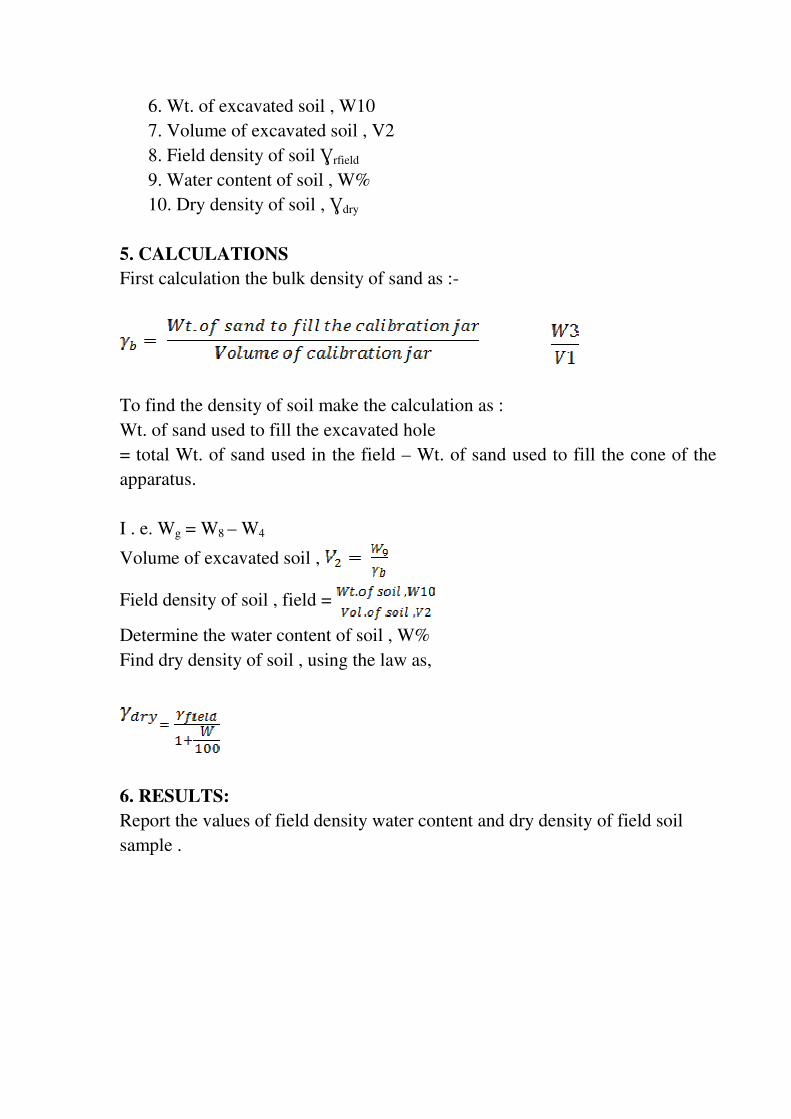
6. Wt. of excavated soil , W10
7. Volume of excavated soil , V2
8. Field density of soil Ɣrfield
9. Water content of soil , W%
10. Dry density of soil , Ɣdry
5. CALCULATIONS
First calculation the bulk density of sand as :-
To find the density of soil make the calculation as :
Wt. of sand used to fill the excavated hole
= total Wt. of sand used in the field – Wt. of sand used to fill the cone of the
apparatus.
I . e. Wg = W8 – W4
Volume of excavated soil ,
Field density of soil , field =
Determine the water content of soil , W%
Find dry density of soil , using the law as,
6. RESULTS:
Report the values of field density water content and dry density of field soil
sample .

EXPERIMENT NO.5
FIELD DENSITY BY BALLOON METHOD
ASTM D-2167
1. AIM
To determine the field density of soil by rubber balloon method.
2. APPARATUS :-
Balloon density apparatus, balance 0.01g sensitivity, oven, chisel
,containers , density plate .
3. PRCCEDURE
3.1 remove base from the density apparatus removing the four socket head
screws with hexagon wrench .
3.2 pass the neck of the balloon through hole in base and then stretch it
over the lip around the hole. Fit wire around the balloon under the lip twist
ends together and fold ends down .
3.3 replace the base and fit socket screws and tighten .
3.4 remove the hexagon headed filler cap . fill unit through the aperture
with clean water until the level is coincident with the top of sighting
window.
Replace filler cap , and tighten in position .
3.5 stand the apparatus on a smooth, flat surface and check for air and
water tightness by pressurizing the system slightly.
3.6 positions the density plate on a smooth flat surface and set the
apparatus into the recess.
3.7 pressurize the system and continue pump until the water level in the
graduated cylinder reaches its lowest point Record the volume shown . this
is initial based reading .
3.8 release the pump and inert the pump to suck the balloon into the
cylinder .
3.9 put the density plate on the surface of the material to be tested and dig
through the hole in the plate to the desired depth .
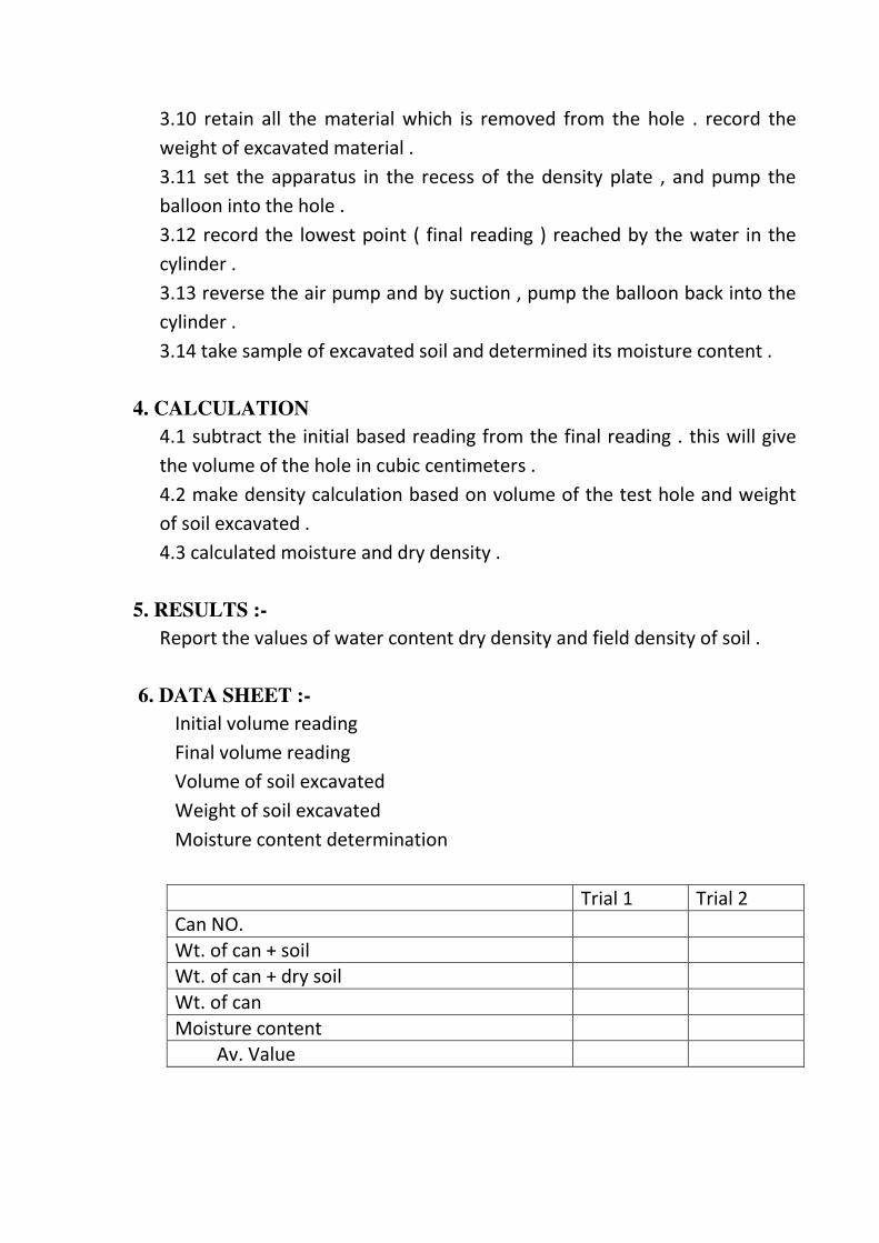
3.10 retain all the material which is removed from the hole . record the
weight of excavated material .
3.11 set the apparatus in the recess of the density plate , and pump the
balloon into the hole .
3.12 record the lowest point ( final reading ) reached by the water in the
cylinder .
3.13 reverse the air pump and by suction , pump the balloon back into the
cylinder .
3.14 take sample of excavated soil and determined its moisture content .
4. CALCULATION
4.1 subtract the initial based reading from the final reading . this will give
the volume of the hole in cubic centimeters .
4.2 make density calculation based on volume of the test hole and weight
of soil excavated .
4.3 calculated moisture and dry density .
5. RESULTS :-
Report the values of water content dry density and field density of soil .
6. DATA SHEET :-
Initial volume reading
Final volume reading
Volume of soil excavated
Weight of soil excavated
Moisture content determination
Trial 1 Trial 2
Can NO.
Wt. of can + soil
Wt. of can + dry soil
Wt. of can
Moisture content
Av. Value
EXPERIMENT NO. 6
LIQUID LIMIT AND PLASTIC LIMIT
ASTM D-4318
1. AIM :-
To determine the liquid limit and plastic limit of soil .
2. APPARATUS :-
Liquid limit device , grooving tool , glass plate balance ( 0.01g sensitivity ),
oven , spatula , wash bottle ASTM sieve No. 40 ( 0.425 mm)
3. PROCEDURE:-
3.1 liquid limit determination
3.1.1 Check the height of fall of the L.L. device . grooving tool has end
block of size 1 cm . it can be used to check the height of fall .
3.1.2 Take a bout 200g of soil passing ASTM sieve No. 40 in aporcetain
dish . add distilled water to soil and mix it thoroughly to form uniform
paste .
3.1.3. Place the soil in the cap of liquid limit device to a maximum depth
of 13mm and level the surface.
3.1.4. Draw the grooving tool through the sample to set asymmetrical
groove in the centre of the cup.
3.1.5 Turn the crank at a rate of two revolutions per second , and count the
blows necessary to close the groove for a distance of 13mm , preferably
observe the no. of blows , must be between 10 and 40 .
3.1.6 Take approximately 10 g of soil from near the closed groove for
water content determination.
3.1.7. Remove the sample from the cup and clean the cup .
3.1.8. By altering the water content of soil and repeating steps 3.1.2. to
3.1.5. Obtain four water content determination and their respective number
of blows.
3.2 plastic limit determinations:-
3.2.1 Mix thoroughly a bout 20g of soil .
3.2.2. Roll the soil on a glass plate with the palm until it is a uniform tread
of 3 mm diameter .
3.2.3. If the soil rolls into thread of less than 3mm diameter, make it a
lump again and reroll it until a thread of 3mm diameter shows signs of
crumbing .

3.2.4. Take some of the crumbling material obtained in step 3.2.3. for a
water content determination .
3.2.5. Replace steps 3.2.2. to 3.2.4. obtain three determinations which can
be averaged to give the plastic limit .
4. CALCULATIONS
In both the experiments of L.L. and P.L. the calculation are made for
water content determination. To find the L.L. plot a graph between no. of
allows on log scale on x – axial and water content on y- axis as shown in
fig (a) find the water content corresponding to 25 blows. This will give the
liquid limit of soil.
From the L.L. & P.L. values calculated the P.I as
PI = L.L. – P.L
5. RESULTS :-
Report the values of L.L. , P.L. and P.I of soil
6. DATA SHEET
Liquid limit :-
NO 1 Trial No. 1 2 3 4
1 Number of blows N
2 Wt. of wet soil + can w1
3 Wt. of dry soil + can w2
4 Wt. of can w3
5 Wt. of dry soil w2-w3
6 Wt. of moisture w1-w2
7 Water content W%
(w1-w2 )/ ( w2 – w3 )


EXPRIMENT NO.7
SHRINKAGE LIMIT
1. AIM:
To determine shrinkage limit of soil sample .
2. APPARATUS:-
Shrinkage dish (circular flat bottom diameter about 44.5 mm and height
about 13 mm).
Evaporating dish
Spatula
Volume measuring apparatus .
Balance 500g capacity and 0.1g accuracy .
Oven.
ASTM sieve no.40 (0.425 mm)
3. PROCEDURE:-
3.1 Take about 40g of soil passing ASTM sieve No.40 (0.425) .In the
evaporating dish .
3.2 Add water to the soil such that soil will become saturated, or the
consistency of soil becomes slightly above liquid limit .
3.3Apply alight coat of petroleum jelly or oil to the inside of shrinkage
dish such coat prevent the soil sticking to the dish.
3.4 Take the weight of empty dish record it .
3.5 Fill the dish with wet soil in the three layer . After each layer top the
dish gently on a firm base so that the soil flows all over the dish to remove
air bubbles .
3.6 After the final layer, make the top surface of the dish level using
spatula clean outside surface of the dish .
3.7 Take the weight of dish filled with wet soil .
3.8 Air dry the path by placing the dish in the laboratory for about 24 hrs .
3.9 After air drying keep the dish in oven for drying After 24 hours record
the weight of dish with dry sample .
3.10 Make the volume measuring apparatus in working condition by
checking he level electrical contact, and amount of mercury .
3.11 Remove the air bubbles trapped in the instrument by lowering the
cage 2-3 times .
3.12 Adjust the micrometer until the bubble just up .Record the reading of
the micrometer .
3.13 Place the oven dried soil pat in the cage and lower it .
3.14 Adjust the micrometer once again after removing trapped air bubbles
,until the bulb just light up . Record the micrometer reading .
4. CACULATION :-
4.1 Calculation the volume of wet soil equal to volume of shrinkage dish
( )
4.2 From the initial wet weight and final dry weight of soil ,Wd demine the
water content of soil ( ).
4.3 From the micrometer reading of the volume measuring apparatus
calculate the dry volume of soil sample ( ) .
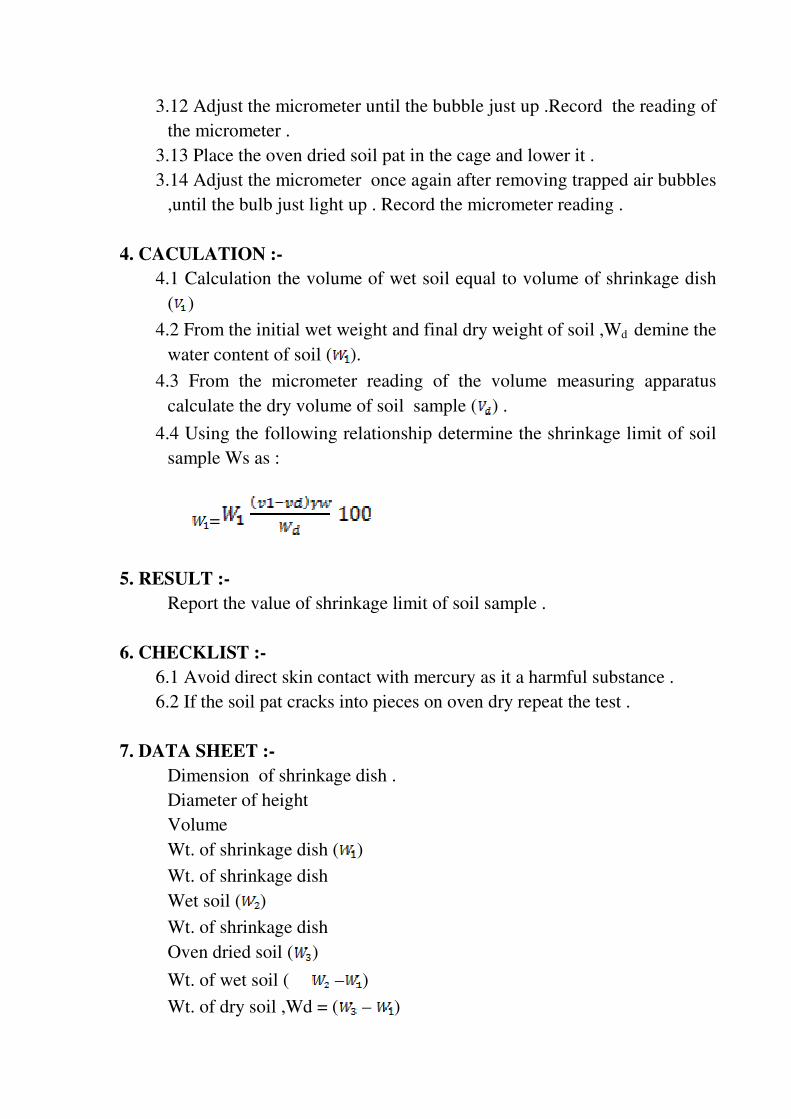
4.4 Using the following relationship determine the shrinkage limit of soil
sample Ws as :
=
5. RESULT :-
Report the value of shrinkage limit of soil sample .
6. CHECKLIST :-
6.1 Avoid direct skin contact with mercury as it a harmful substance .
6.2 If the soil pat cracks into pieces on oven dry repeat the test .
7. DATA SHEET :-
Dimension of shrinkage dish .
Diameter of height
Volume
Wt. of shrinkage dish ( )
Wt. of shrinkage dish
Wet soil ( )
Wt. of shrinkage dish
Oven dried soil ( )
Wt. of wet soil ( – )
Wt. of dry soil ,Wd = ( – )

Initial water content ,
Micrometer reading , initial
Micrometer reading , final
Volume of dry soil ,
Shrinkage limit ,
EXPERMENT NO.8
STANDARED PROCTOR TEST
ASTM D-698
1. AIM :
To determine the relationship between dry density and water content to
obtain maximum dry density and optimum moisture water content for a
soil.
2. APPARATUS :-
Standard Proctor mould with base plate and collar.
Rammer weight 2.5 kg with fall of 30 cm .
ASTM sieve NO.4(0.425) .
Sample extruder
Tray for mixing soil .
Measuring cylinder 500 ml capacity
Balance (capacity 15kg .acuracy1g )
Balance (capacity 200g accuracy 0.01g)
3. PROCEDURE :-
3.1 Take about 3 kg of air dry soil passing ASTM NO.4 sieve .
3.2 Weight empty with base plate but without collar .
3.3 Determine the volume of mould by measuring its diameter and height .
3.4 Add about 4 % water by weight i.e. about 120g (120 ml) to the soil .
mix the water thoroughly with soil .
3.5 Compact the soil in the proctor mould . The compaction is done in 3
layers, and each layer is given 25 blows of rammer .the third layer
should be about 6 mm .above the top of mould projecting into collar
after compaction .
3.6 Remove the collar and termite top compacted soil level to top of the
mould by straight edge .
3.7 Recode the weight of the mould with its base plate and compacted soil
(W2).
3.8 Remove the soil from the mould , of necessary by using soil extruder .
collect two samples for water content determination .
3.9 Break the soil into small pieces . Add again about 4 % water by
weight to the soil and mix it thoroughly .

3.10 Repeat step 3.5. TO 3.9 till weight of mould with compacted soil
decreases .
4. CALCULATIONS :-
From the wet weight (W2 –W1) and volume if soil (equal to volume of
mould ) wet density ,Ɣ wet of soil can be calculated as :-
V : Further dry density of soil calculated using the relationship ,
5. RESULTS :-
Plot a graph between moisture content on X -axis and dry density on Y-
axis . From the graph the maximum dry density and corresponding
optimum moisture content .
6. CHECKLIST
3.10 After adding water to sold , mixing of soil is done thoroughly .
3.11 Rammer ,while compacting should be moved on the entire
surface of in the mould .
3.12 After compacting 1 st and 2nd
layer make some scratches on the
surface of soil for good bond .
7. DATA SHEET :-
Mould dimension : Volume : Height:
(i) Moisture content determination :
Sr.No
.
Trial No. 1 2 3 4 5
1 Can No.
2 of empty can
3 of can + wet soil
4 of can + dry soil
5 of moisture
6 of dry soil
7 % Moisture content
8 % Av . Moisture
content

(ii) Density determination :
Sr.No. Trial No. 1 2 3 4 5
1 of empty mould =
2 of mould + wet soil
=
3 of wet soil = -
4 Wet density of soil =
5 Moisture content = W
6 Dry density of soil =

EXPERMENT NO. 9
CONSTANT HEAD PERMEBILITY TEST
ASTM D-2434
1. AIM
To determine the coefficient of permeability of sand sample by constant
head permeability test .
2. APPARATUS :-
Permeameter
Constant head reservoir
Stand pipes
Source of water supply
Stop clock ( watch)
Measuring jar
Spatula
Slide calipers, scale
3. PROCEDURE
3.1 Measure the inner diameter of permeameter and the vertical distance
between intake point for piezometer observations .
3.2 Open the water supply and fill up the permeameter by letting water in
through constant head reservoir .
3.3 See that there is no air entrapped in the leads from piezometric in take
points in the permeameter .Shut down the flow of water into
permeameter .
3.4 Deposit through water a layer clean well graded coarse filter material
at the bottom of the permeameter . Speared it and gently compact it
with a spatula or a rod . The top of filter material should be below the
level of bottom intake point for piezometric observation .
3.5 Deposit a few spoons ful of sand through standing water in the
perfmeameter . The sand must have been washed before ,boiled ,
cooled and kept submerged in water . Compact the sand using spatula
or rod to the required extent . The sample inside permeameter is built
up in layer and should extend a little beyond the level of top intake
point for piezometric observations .

3.6 Deposit a layer of filter material at the top of sample . It must be built
up to level to allow the cover at the top to rest on the filter and the
permeameter .
3.7 Place the cover at the top and tight it with screws
3.8 Open the valve slightly to allow flow of water into permeameter . The
water allows through soil and comes out at the top . The water level in
stand pipe also rises and register pressure at intake point . Watch for the
reading in stand pipe to stabilize .Collect the water from top in a
measuring jar for a fixed time interval . Record the observation for
quantity of water collected and reading on the stand pipe. Repeat the
observation for quantity of water collected and the reading on the stand
pipe .Repeat the observation till reading are consistent . While making
the observation constant head must be maintained in water reservoir .
This will be evident by continuous flow water in the overflow pipe .
3.9 Repeat step 3 .8 three or four time by varying the discharge of water
through soil . This can be controlled by keeping the valve open at
different positions .
4. CACULATIONS
Head loss in col. (5) is = . K in col (6) is calculated
from :
K =
Report the average value of coefficient of permeapility of sand sample
5. CHECK LIST
a. Ensure that there is no air enterapped in the leads from piezometer
intake points .
b. There must be continuous overflow of water in the over flow pipe
to maintain constant head .
c. There must be no leaking in the permeameter .
6. DATA SHEET
Inner diameter of permeameter (D) :
Area of soil sample (A= )
Distance between bottom and top intake point for piezometric

observations (L) :
Elapsed
time
Discharge
Q
Reading in stand
pipe
Head
loss
K
(1) (2) bottom top (5) (6)
(3) (4)

EXPERIMENT NO.10
VARIABLE HEAD PERMEAPILITY
1. AIM
To determine the coefficient of permeability of soil by variable head test .
2. APPARATUS :
Permeameter mould
stand pipe
vacuum supply
stop clock (watch)
spatula
3. PROSEDURE
3.1 Measure the inside diameter of the stand pipe , and the height and inner
diameter of permeameter . weight and record the empty weight of
permeameter
3.2 Fill the permeameter soil sample and trim both ends. Determine the
weight of the permeameter with the soil sample . From trimmings at the
ends determine the water content of soil .
3.3 Place the cover at top and the wire gauze at the bottom and fix the
permeameter to it base .
3.4 Keep the bottom of permeameter slightly below water level in a tray
filled with water .
3.5 Through top of permeameter mould apply vacuum for about 20-30
min. to saturated soil sample .
3.6 Remove vacuum supply and connect the stand pipe to permeameter .
Water must be at sufficient level in stand pipe. It must be ensured that
no air gets entrapped in stand – pipe or in the permeameter .
3.7 Record the difference in the levels of water in stand pipe and water in
the tray .
This the initial head loss in the soil sample . Start the stop watch .At
different elapsed times record the difference in the two water level .
3.8 Remove the soil from permeameter and determine its moisture water
content .
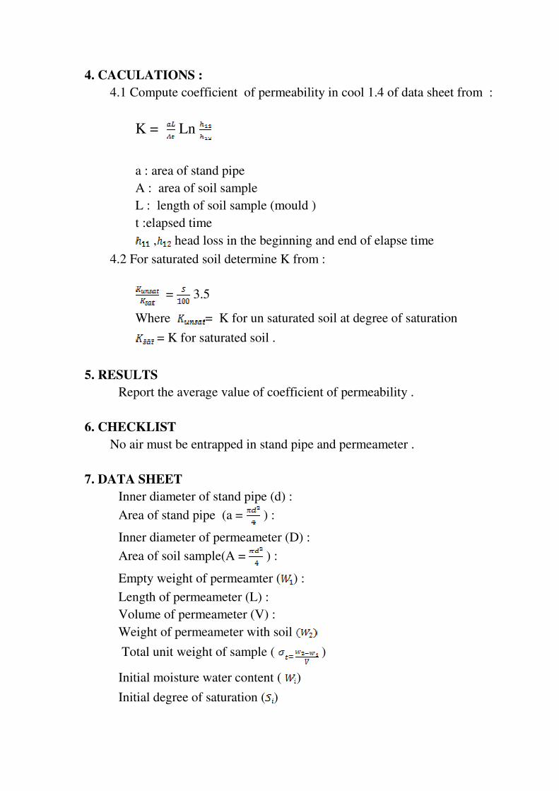
4. CACULATIONS :
4.1 Compute coefficient of permeability in cool 1.4 of data sheet from :
K = Ln
a : area of stand pipe
A : area of soil sample
L : length of soil sample (mould )
t :elapsed time
, head loss in the beginning and end of elapse time
4.2 For saturated soil determine K from :
= 3.5
Where = K for un saturated soil at degree of saturation
= K for saturated soil .
5. RESULTS
Report the average value of coefficient of permeability .
6. CHECKLIST
No air must be entrapped in stand pipe and permeameter .
7. DATA SHEET
Inner diameter of stand pipe (d) :
Area of stand pipe (a = ) :
Inner diameter of permeameter (D) :
Area of soil sample(A = ) :
Empty weight of permeamter ( ) :
Length of permeameter (L) :
Volume of permeameter (V) :
Weight of permeameter with soil
Total unit weight of sample ( )
Initial moisture water content ( )
Initial degree of saturation ( )
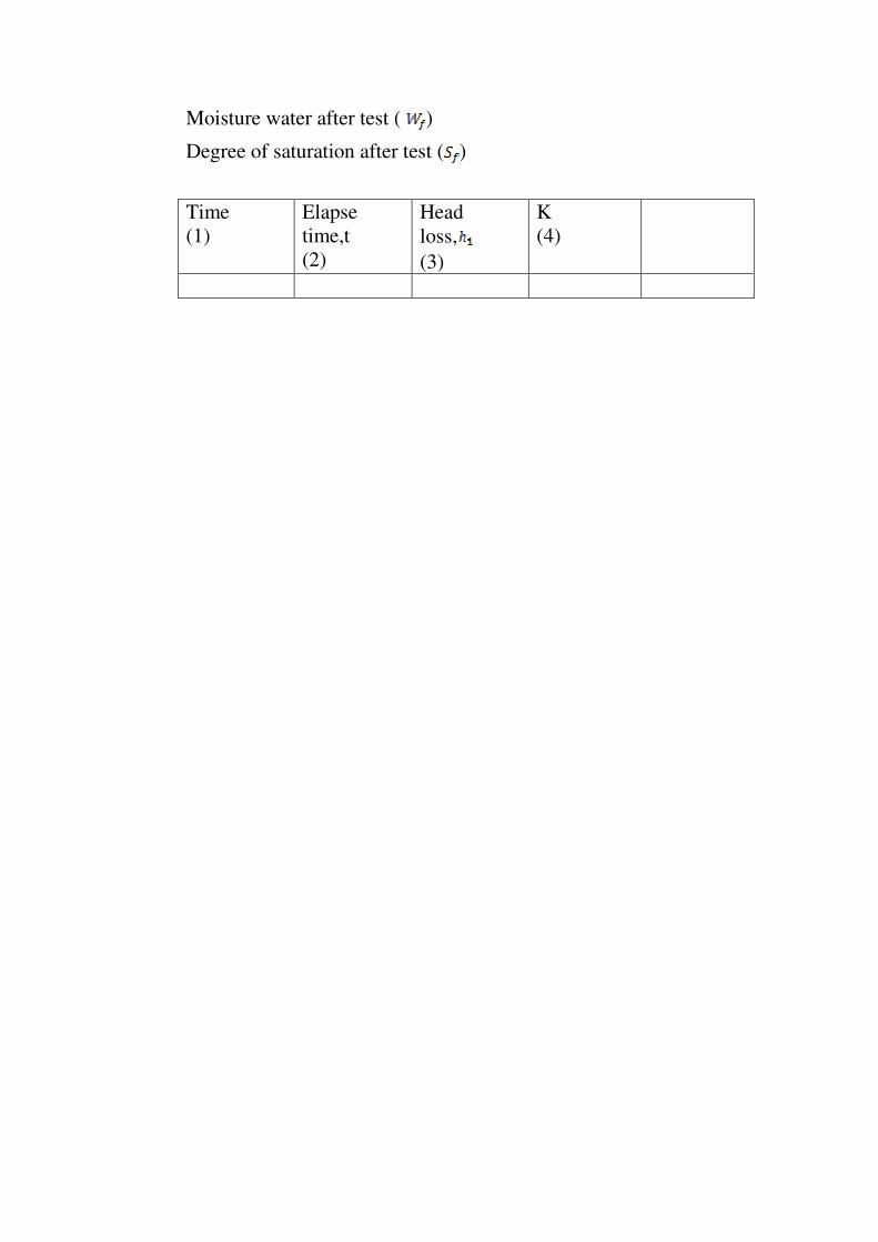
Moisture water after test ( )
Degree of saturation after test ( )
Time
(1)
Elapse
time,t
(2)
Head
loss,
(3)
K
(4)
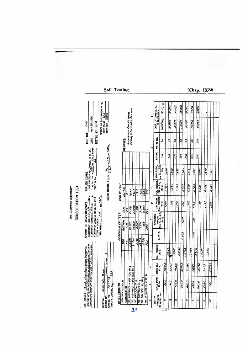
EPERMENT NO.11
CONSOLODATION TEST
ASTM D-2435
1. AIM :
To determine the consolidation characteristics of a given soil sample .
2. APPRATUS :
Consolidation unit , specimen trimmer and accessories . Device
sensitivity ) ,Oven, Descater Timer , moisture content cans Evaporating
dish .
3. PRUSEDURE
3.1- Specimen preparation :-
1- Measure the height and inner diameter of the consolidation ring .
Also measure the combined thickness of the upper porous stone and
cover .
2- Determine the weight of whose parts which lie on the top of the
specimen to add it to computed scale load required to give the
desired pressures .
3- Trim the test specimen by using a special sample trimmer.
4- From the soil trimmings obtain at least three representative specimen
for water content determination .
5- Place the trimmed specimen in the container carefully .
6- Trim the top and bottom faces of the specimen by means of a wire
sawer knife .
7- Place the specimen and the container on the porous stone which has
been soaked in water on the base of the unit , and then raise the water
level above the porous stone .
8- Place the specimen and the container on the porous stone and
carefully place the ring seal , porous stone and cover on top o the
soil specimen .
3.2 Compression Test :
1. Mount the container with specimen in the loading unit .
2. Screw the holder with vertical deflections dial in place and adjust it
in such a way that dial is the beginning of its release run .
3. Apply the load to give a pressure intensity of 0.1 on the soil
specimen , and start taking time and vertical deflection reading .
Compression reading should be taken at total elapsed times of
0, ,1, ,4, ,9, ,6, ,, ,25 minutes etc . until 90% consolidation
has been reached . This point can be determined by the square root
fitting method .
4. At the end of 24hr ,a compression and time reading should be made
and then the load increased to 0.25 and step 3.2.3 is repeated
. Like wise the following further load increments are made on the
soil sample :
0.5 , 1 , 2 , 4 and 8 .
5. After the 8 load has been on for 24hr , the load is decreased
to 2 and then 0.1 rebound loads .
6. After the final reading has been taken for the 0.1 load .quickly
dismantle the apparatus dry the surface water of the soil specimen
and weight .
7. Place the weight specimen in the oven to dry for water content
determination .
4. CALCULATION :-
The calculation of the consolidation test result are shown in the columns of
the data sheet which is as follows :
Col . a- The pressures to which the specimen is to be subjected
b. Its obtain by adding the tare weight to the product of the specimen
area and the desired pressure intensity .
c. The final vertical dial reading for each load .
d. The change in final dial readings is the compression for load
increment and is found by subtracting successive numbers in column
(CA) .
e. Computed 2H values by means of the dial value form column d .
f. The void weight found by subtracting the height of solids , 2Ho
,from the specimen height, 2H, read from col(2) The of 2Ho is found
from ,
2Ho =
Where = weight of solids
G = specific gravity
A = The area of sample
g. The void ratio ,e, is equal the void height divided by height of
solids .
e = =
h. In this column are listed the time for 90% of primary compression
if the square root fitting method is used or the time for 50% of
primary compression if the log the fitting method is used .
I. The coefficient of consolidation Cv is computed from the following
equation :
a. Square root fitting method L:Cv =
b. Log fitting method Cv =
In Eqs , 1&2 His the average thickness . it is found by dividing the sum
of the 2H value (col.e) for boundary loads of the increment by four .

EXPERMINT NO .12
DIRECT SHEAR TEST
ASTM D-3080
1. AIM
To conduct a direct shear test on a dry sand specimen to determine its
shear strength parameter .
2. APPARATUS
Direct shear box and accessories – a metal box in two halves , bottom
plate ,metal plates with serration , locking pins , loading cap , spacing
screws .
Direct shear machine – with facilities to apply normal and shear load on
the shear and vertical displacement of the soil sample slide calipers .
Balance – 2 Kg capacity accuracy 1g
3. PROCEDURE
a. Measure the plan dimension of the shear box .
b. Insert the bottom plate .
c. Secure the two halves of the shear box together with the locking
pins .
d. Measure the average thickness of serrated plates .
e. Insert a serrated plate and make it rest on the bottom plate such
that the serrations are at right angle to the movement of the box .
f. Measure the average height available inside the box for
preparation of soil sample .
g. Measure the empty weight of the shear box with bottom plate ,
locking pins and serrated plate .
h. Place sand inside the shear box in little quantities and and
compact each layer uniformly with a tin rod .
i. Build up the sand sample till it reaches thickness 10 to 12 mm
inside the top half of the shear box .
1-Level up the surface of sand .
2-Insert another serrated plate on top and make it rest firmly on the
sand . The serration must at right angle to the direction of shear
displacement . The average thickness and weight of the serrated
plate should have been measured earlier .

3-Measure the average height inside the box above the top serrated
plate .
4-Weight the shear box at this stage .
5-Place the loading cap at top and place the shear box in the
container in the direct shear machine .
6-Place the loading yoke on the loading cap and apply a
predetermined value of vertical load on the soil sample .
7-Adjust the machine such that initially there is on shear load on
the soil but will start building up immediately after the machine is
suited on .
8-Using the spacer the two halves of the shear box slightly to
eliminate the contact friction at the inter face .
9-Set the horizontal dial gauge to measure the shear displacement
and the vertical displacement of the sample .
10-Set rate of movement . For dry sand use a rate of displacement
of .
11-Note the initial reading in the horizontal , proving ring and
vertical dial gauges .
12-Remove the locking pins .
13-Switch on the machine and record the proving ring and vertical
dial gauge reading at regular intervals of horizontal dial reading .
14- Continue the observations until failure is reached or until the
shear displacement equals 15% of the length of the sand sample .
Repeat the test for three or more normal load on the sample.
4. CACULATION
In data sheet col. 1,2 and 3 are observed. Shear displacement in Col. 4 is
obtained from col. 1 and least count of horizontal dial gauge . shear load
is entered on Col. 5 from reading in Col.6 is calculation as = shear load
in col.5 /(LxB) . Vertical displacement (4h) in col. 7 is obtained from
vertical dial gauge reading in col. 3 and its least count value . +ve sign is
used for compression and –ve for expansion – volumetric strain in Col 8
is obtained as x 100 . Where h is the thickness of sand sample.
From result the maximum value for shear stress , max , can be observed .
The angle of shearing resistance , is computed as
=
Where = normal load intensity .
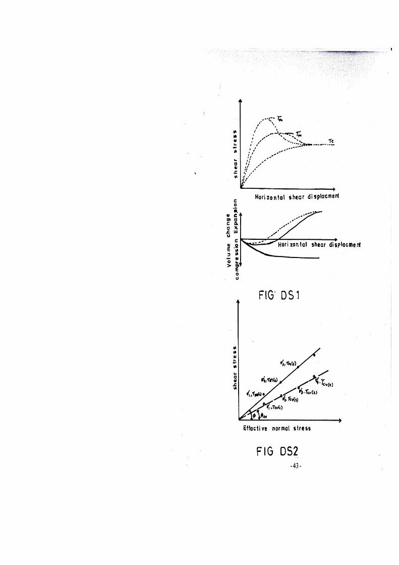
5. RESULTS
1- Plot shear displacement vs .shear stress and displacement vs .
volumetric strain curve as shown in Figure DS 1 .
2- Plot the failure envelope as shown in Figure DS 2 .
6. CHECKLIST
1-See whether all the data for calculation of density have been entered
before shearing the sample
2- Remove locking pins before applying shear load .
3- While repeating the test for different normal loads it must be
ensured that all the sample have nearly the same density.
7. DATA SHEET
DIRECT SHEAR TEST
Plan dimension of Shear box (LxB) : ………. …………
Height available for preparation
Of soil sample ( ) : ……………………………
DS Machine No.: ………………..
Proving ring No. : ………………..
LC of horizontal dial gauge : …………
Weight of empty shear box ( ) : …….
LC of vertical dial gauge : ……………
Thickness of top serrated plate (t) ………….
Height of box above the serrated plate at top ( ) : ……………
Thickness of soil sample (h = t - ) : ………………..
Weight of shear box with sand ( ) : ……………………..
Weight of sand (w = - ) : …………………..
Density of sand ( : ………………………….
Normal pressure on soil sample : ……………………
Shear
displacement
dial gauge
(1)
Proving
ring
reading
(2)
Vertical
dial gauge
reading
(3)
Shear
Displacement
(4)
Shear
load
(5)
Shear
stress
(6)
Vertical
displace
ment
(7)
Volumetric
strain %
(8)

EXPERIMENT NO.13
Unconfined Compression Test
ASTM D-2166
1-AIM
To Carry out unconfined compression test on a soil sample and determine its
compressive strength or undrained shear strength.
2- APPARATUS
Unconfined compression testing machine with proving ring.
Triaxial cell
Weighing balance – 200 gms capacity accuracy 0.01 g.
Moisture cans
Oven
Desiccators
Perspex or impervious disc
Perspex or impervious loading cap
3-PROCEDURE
3.1 Prepare a soil specimen of standard dimensions,38 mm diameter and 76
mm long.
3.2 Collect the trimmings from the ends of the soil sample and determine the
moisture content.
3.3 Weigh the soil sample
3.4 Place an impervious disc on the pedestal of the triaxial cell base.
3.5 Place the soil sample on the impervious disc.
3.6 Place an impervious loading cap at the top of the sample.
3.7 Place the triaxial cell over the base and tighten the screws.
3.8 Transport the cell with the soil sample to the load frame.
3.9 Adjust the load frame such that the proving ring and the ram of the cell are
in /contact with each other without exerting axial load on the soil sample .
3.10 Set the rate of displacement. For unconfined confined compression test,
rate of displacement can be computed on the basis of reaching 15% axial strain
in 20 to 30 minutes.
For a standard sample of 76 mm length , the rate of displacement varies from
0.38 mm/min to 0.57 m/m min
3.11 Set the vertical displacement measuring dial gauge.
3.12 Note down the initial reading in the vertical displacement dial gauge and
in the proving ring dial gauge.
3.13 Switch on the machine and record the proving ring reading at regular
intervals of vertical displacement dial gauge reading.
3.14 Switch off the machine when the soil sample has failed or when the axial
strain has reached a value of 15 %
4. CALCULATIONS:
COI.1 and 2 in data sheet are recorded observations. Vertical displacement ∆
L in col.3 is obtained from reading in col. 1 and the least count of vertical
displacement dial gauge . Compute axial strain as ϵ1 = ∆L / Lₒ and enter
in col . 4. Corrected area in col . 5 is calculated from
A1 = A ₒ /(1- ϵ1) where A is the initial area of the soil sample.
Axial load Pa in col .6 is obtained from readings in col . 2 and the calibration
chart of the proving ring. Compute axial stress using the equation .
1 A / Pa = 1σ
And enter in col . 7.
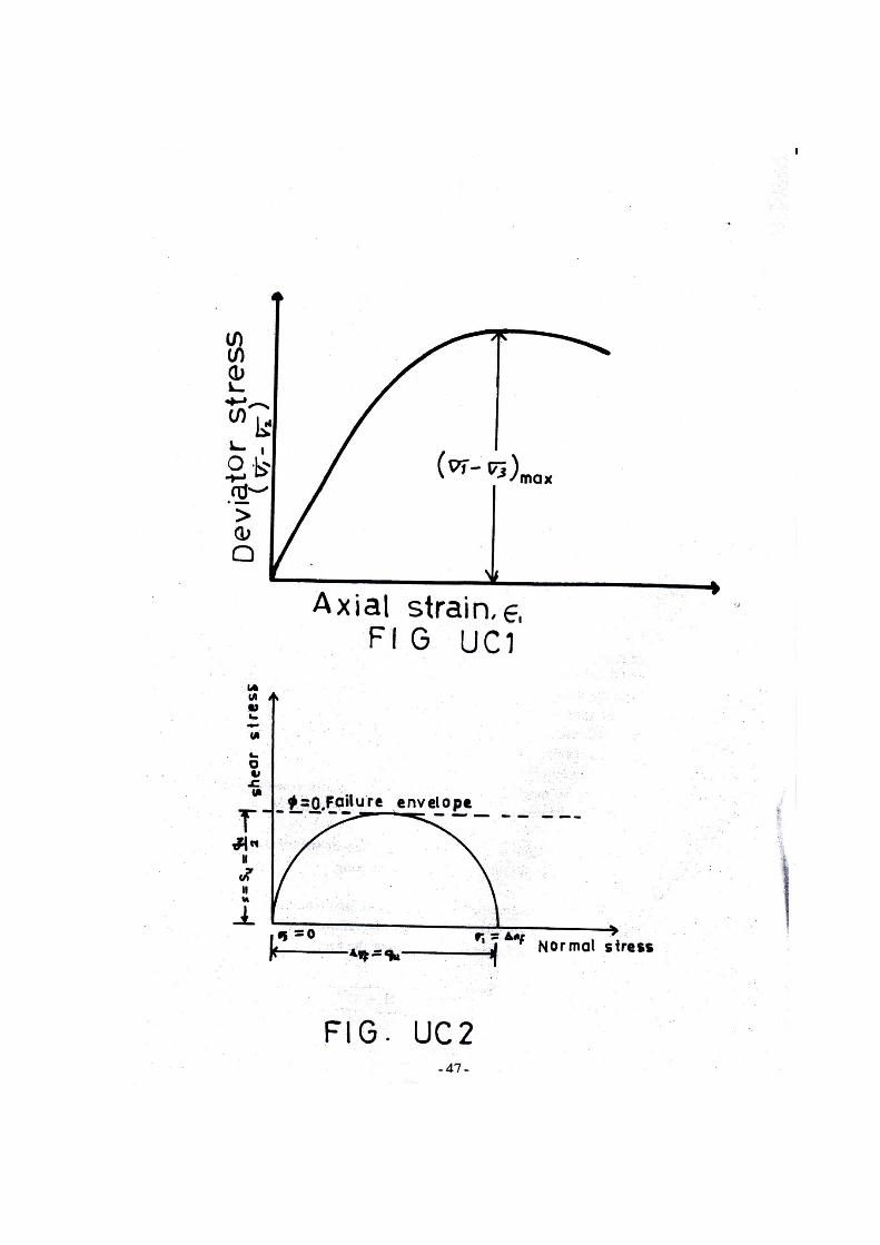
5. RESULTS
Plot σ 1 vs . curve as shown in fig UC1
Plot the Mohr's circle as shown in fig UC2
Compute the undained shear strength (Su) from,
Su=
6. CHCKLIST
6.1 Check whether the ram of the cell falls freely due to its own weight
6.2 Do not touch the ram of the sells
6.3 While placing the cells on the base hold the ram up so that it does not
dissturb the soil sample.
6.4 Where brittle failure is expected keep a constant watch on proving and
vertical displacement dial gauge to record the failure load and displacement.
7. DATA SHEET
Initial dimensions of soil sample:
Diameter (Dₒ):π
Length (Lₒ):π
) 4 / ² = π DDₒArea
(Aₒ
Volume (Vₒ=π) D(D ₒ ² Lₒ)
Weight (Wₒ):
Machine No:
Proving ring No:
LC of vertical dial gauge:
LC of proving ring dial gauge:
Moisture Content Measurements:
Can No:
Weight of can :
Can + Wet soil:
Can + dry soil:

Moisture Content (W):
Unit weights of soil Sample :
Total unit weight (Ɣt = Wₒ / Vₒ):
Dry unit weight (Ɣd = Ɣt / (1+w)):
Axial
Stress
1 σ
(7)
Axial
Load
Pa
(6)
Corrected
Area
A1
(5)
Axial
Strain
ϵ1
(4)
Vertical
displacement
(∆L)
(3)
Proving
ring
reading
(2)
Vertical
displacement
dial gauge
Reading
(1)

EXPEIMENT NO. 14
VANE SHEAR TEST
ASTM D-2166
1. AIM
To conduct vane shear test in the laboratory to determine the undrained strength
of soil.
2. APPARATUS:
Laboratory vane shear apparatus with vanes and rotating mechanism Moulds
for soil Sample
Weighing balance (capacity , accuracy)
Oven
Slide calipers
Moisture cans
Spatula
3. PROCEDURE
3.1 Measure inner diameter and height of mould.
3.2 Record empty weight of mould. Measure dimensions of vane.
3.3 Prepare a soil sample in the mould and trim both ends. Weight the mould
with soil.
3.4 Place the mould in the van shear apparatus and secure it in position.
3.5 Fix the vane to the shear apparatus.
3.6 Insert the vane in to the soil sample to sufficient to ensure shear in soil at
both ends cylinder formed by vanes.
3.7 Record the initial reading in the indicator.
3.8 Switch on the machine which rotates the vane at a constant rate.
3.9 Failure is indicated by a constant reading in the indicator. Record this final
reading.
3.10 Take out the vane and after cleaning it repeat the experiment from other
end of the mould if it is sufficiently long.
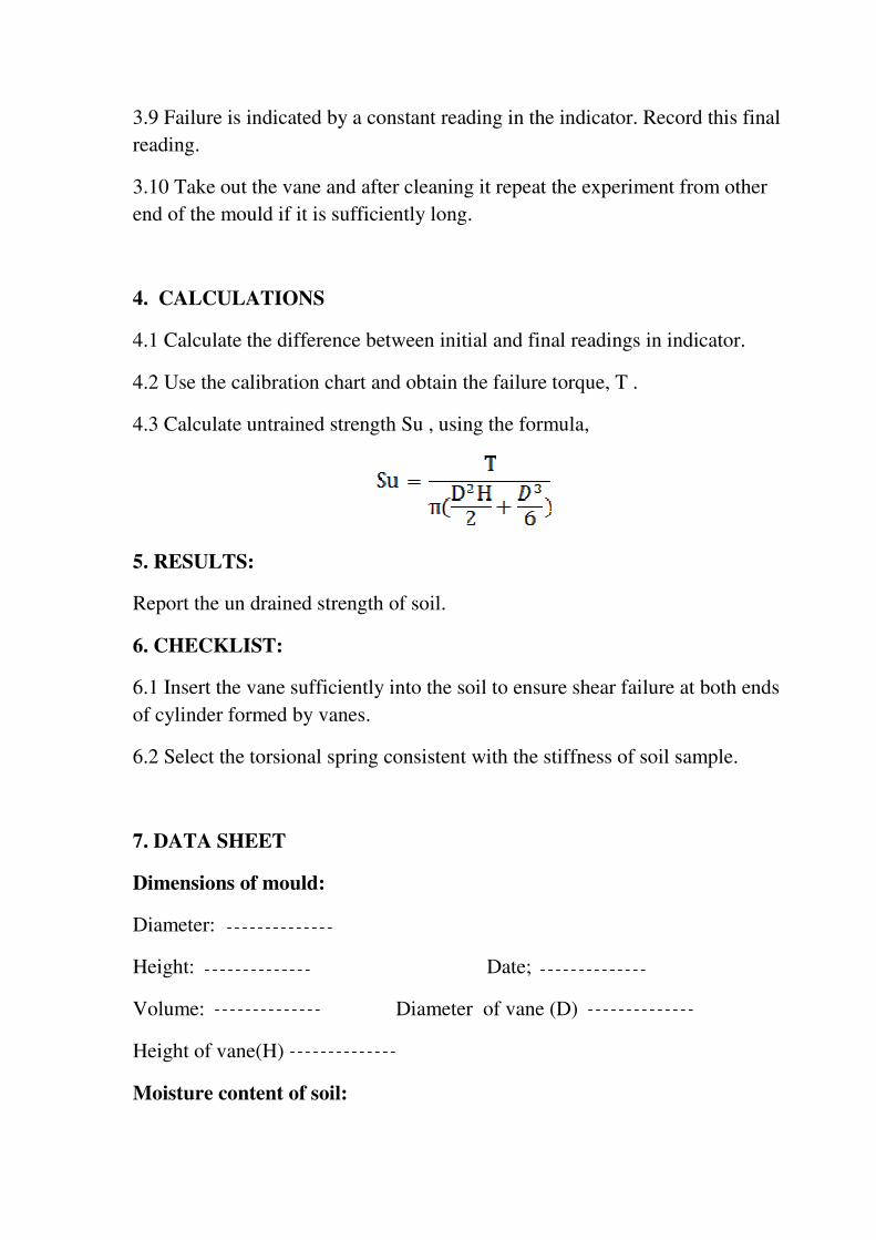
4. CALCULATIONS
4.1 Calculate the difference between initial and final readings in indicator.
4.2 Use the calibration chart and obtain the failure torque, T .
4.3 Calculate untrained strength Su , using the formula,
5. RESULTS:
Report the un drained strength of soil.
6. CHECKLIST:
6.1 Insert the vane sufficiently into the soil to ensure shear failure at both ends
of cylinder formed by vanes.
6.2 Select the torsional spring consistent with the stiffness of soil sample.
7. DATA SHEET
Dimensions of mould:
Diameter:
Date; Height:
Diameter of vane (D) Volume:
Height of vane(H)
Moisture content of soil:

Weight of empty can:
Can +Wet soil:
Can + dry soil:
Moisture content (W):
Unit weight of soil:
Empty weight of mould:
Mould + wet soil:
Total unit weight:
Dry unit weight:
Initial reading in indicator:
Final reading in indicator:
Difference:
Failure Torque:
Undrained strength:
Spring No:

FIG VS1

EXPERIMENT NO. 15
UNCONSOLIDATED UNDRAINED TEST
ASTM D-2850
1.AIM
To determine the shear strength parameters of soil under unconsolidated
undrained situations.
2. APPARATUS:
Loading frame with proving ring
Triaxial cell
Constant cell pressure application system
Weighing balance – 200 gm capacity
Moisture cans
Rubber membrane. 0 – rings,
Membrane stretcher
Perspex or impervious disc
Perspex or impervious loading cap
Oven
Desiccators
3. PROCEDURE:-
3.1- Prepare a soil of standard dimensions, 38 mm diameter and 76 mm
long. Weigh the sample.
3.2- Collect the trimmings from the ends of the soil sample and
determine the moisture content.
3.3- Place an impervious disc on the pedestal of the triaxial cell base.
3.4- Place the soil sample on the impervious disc. and place an
impervious Loading cap at top of the sample.
3.5- Stretch the rubber membrane over the soil sample, pedestal and
loading cap using rubber membrane stretcher.
3.6- Place O- rings on the membrane, two at bottom on the pedestal and
two at top on the loading cap.
3.7- Place the triaxial cell over the base and tighten the screws.
3.8- Transport the cell with the soil sample to the loading frame.
3.9- Connect the hose from de- aired water reservoir to the inlet value at
the base of the triaxial cell. Open the inlet value and fill the cell with
water.
3.10- Develop the required pressure in the constant pressure system and
transfer it slowly to the triaxial cell.
3.11- Record the proving ring reading while it hangs free.
3.12-Adjust the load frame such that proving ring and the ram of the cell
are in contact with each other.
3.13- Lower the ram of the cell till it comes into contact with the loading
cap. The proving ring reading will increase in the beginning of
downward movement, then the reading will become constant. When the
ram comes into contact with the loading cap the proving ring reading
increase again . Stop at this stage.
3.14- Set the rate of displacement. For unconsolidated undrained test.,
rate of displacement can be computed on the basis of reaching 15% axial
strain in 20 to 30 minutes. For a standard sample of 76 mm length, the
rate of displacement ranges from 0.38 mm/min to 0.57 mm/min.
3.15- Set the vertical displacement measuring dial gauge.
3.16- Note down the initial reading in the vertical displacement dial
gauge and in the proving ring gauge.
3.17- Switch on the machine and record the proving ring reading regular
intervals of vertical displacement dial gauge reading.
3.18- Switch off the machine when the soil sample has failed or when the
axial strain reaches a value of 15%.
3.19- Release the load on the proving ring and make it free. Releas the
cell pressure and empty the water in the cell. Remove the soil sample.
3.20- Repeat the test at two or more cell pressures.
4.CALCULATION:
Col.1 and 2 in data sheet are recorded observations . vertical
displacement ∆L in col. 3 is obtain from reading in Col. 1 and the
Least count of vertical displacement dial gauge. Compute axial strain as ,
ϵ1 L=∆L/ To and enter in Col . 4 Corrected area in Col. 5 is calculated
from A1= AAₒ/(1-ϵ1).Axial Load Pa in col. 6 is obtained from readings in
Col. 2 and the calibration chart of proving ring. Deviator load Pd in col. 7
is obtained as, Pd=Pa-(ƿ3xAr),where , Ar is the area of ram. Compute
deviator stress using the equation,

σ 1- σ 3=Pd/A1
and enter in Col,8.
5. RESULTS:
Plot (σ1 –σ 3) Vs.ϵ1 curve as shown in fig. UU1 plot the
Mohr's circles and the failure envelope as shown in fig UU2.
Compute the undrained strength (Su) as
For φu = O̊ conditions.
6. CHECKLIST:
6.1- Check for punctures in the rubber membrane.
6.2- Check whether the ram of the cell falls freely due to its own weight.
6.3- Do not touch the ram of the cell.
6.4- While placing the cell on the base, hold the ram up so that it dose not
disturb the soil sample.
7. DATA SHEDT:
UNCONSOLIDATEP UNDRAINED TEST
Initial dimensions of soil sample:
Diameter (Dₒ):
Length (Lₒ):
Machine No:
Area (Aₒ = π D˳² / 4):
Proving ring No: Volume (Vₒ = π Dₒ ²Lₒ ):
L C of vertical Weight (Wₒ):

Dial gauge: Moistur Content measurements:
L C of proving Can No:
Ring dial gauge: Weight of can:
Cell pressure(σ 3): Can + wet soil:
Proving ring Can +dry soil:
Reading while free: Moisture content (W):
Diameter of ram(Dr): Unit weight of soil sample:
Rate of displacement: Total unit weight (√ t = Wₒ / Vₒ):
Dry unit weight, √ d = √ t / (1+ w):
Deviato
Stress
(σ1 –σ)
(8)
Deviator
Load
Pd
(7)
Axial
Load
Pa
(6)
Corrected
Area
A1
(5)
Axial
Strain
ϵ1
(4)
Vertical
Displace-
Ment
(∆L)
(3)
Proving
Ring
Reading
(2)
Vertical
displace
ment
reading
(1)

EXPERIMENT NO. 16
CONSOLIDATED DRAINED TEST ON SAND
ASTM D-422
1.AIM
To determine the shear strength parameters of sand under drained conditions of
loading.
2. APPARATUS:
Loading frame with ring
Triaxial (cell)
Constant cell pressure application system
Split sampler
Porous discs
Rubber membrane
O – rings
Burette
Perspex or impervious loading cap
Weighing balance
Oven
Spoon
Thin rod – 3 mm diameter, fitted with rubber
Cushion at one end.
Slide calipers
3. PROCEDURE
3.1- Measure the depth of the pedestal of the cell base, the thickness of porous
disc and the thickness of the impervious loading cap

3.2- Stretch a rubber membrane over the pedestal – of the cell .. place two O-
rings on the membrane.
3.3- Place the split sampler on the base around the pedestal enclosing the rubber
membrane.
3.4- Stretch the rubber membrane over the split sampler.
3.5- Connect a burette with water to one of the two values in the base which
leads to one of the two openings in the pedestal. Open and shut this valve a few
number of times to remove the air in the opening.
3.6- Open and shut the other valve in the base which loads to the other opening
in the pedestal , a few number of times. This drains out some water from the
split sampler and de- airs the other opening.
3.7- Fill up the split sampler with water.
3.8- Keep all the valves in the base shut.
3.9- Insert a porous disc through split sampler and place it on the pedestal.
3.10- Take sand using a spoon from a container , in which the preboiled sand is
kept immersed in water , and place it in side the split sampler.
3.11- After placing a few spoons of sand compact the sand using a rubber
sheathed thin rod.
3.12- When the sampler reaches to the top of the sampler, make the surface
level. Place the loading cap and gently press it slightly into the split sampler.
3.13- Using wash bottle wash off the sand particles on the membrane at the top
of the sampler.
3.14- Stretch the membrane over the loading cap and place two O- rings.
3.15- Take the burette down by about 1 m. It can be kept on the floor.
3.16- Open the valve connecting the burette to the sand sample.
3.17- Remove the split sampler.
3.18- Wash the sand sampler and the base of the cell to remove sand particles
outside.
3.19- Measure the average initial diameter of the sample, by taking
measurements near the top, middle and bottom of the soil sample.
3.20- Measure the height from top of loading cap to bottom of pedestal.
3.21- Place the triaxial cell over the base and tighten the screws
3.22- Close the valve connecting the burette to the sand sample.
3.23- Transport the cell with the sand sample, and the burette to the loading
frame.
3.24- Connect the hose from de- aired water reservoir to the inlet valve at the
base of the triaxial cell.
3.25- Open the inlet valve and fill the cell with water.
3.26- Keep the burette at the same level as the cell and open the valve to the
burette.
3.27- Adjust the burette such that the water level in the burette is approximately
at the mid – level of the sample.
3.28- Close the valve to the burette ,. Note down the reading in the burette.
3.29- Develop the required pressure in the constant pressure system and transfer
it slowly to the triaxial cell.
3.30- Open the valve to the burette.
3.31- Wait until the water level in the burette stabilises and record the reading.
3.32- Record the proving ring reading while it hangs free.
3.33- Adjust the load frame such that the proving ring and the ram of the cell
are in contact with each other.
3.34- Lower the ram of the cell till comes into contact with the loading cap. The
proving ring reading will increase in the beginning of downward movement,
then the reading will become constant.
When the ram comes into constant with the loading cap the proving ring
reading will increase again.
Stop at this stage.
3.35- Set the rate of displacement. For drained test on sand, the rate of
displacement can be computed on the basis of reaching 15 % axial strain in 30
minutes.
3.36- Set the vertical displacement measuring dial gauge.
3.37- Note down the initial readings in the vertical displacement dial gauge in
the proving ring , and in the burette.
3.38- Switch on the machine and record the proving ring reading and burette
reading at regular intervals of vertical displacement dial gauge reading.
3.39- Switch of the machine when the soil sample has failed or when the axial
strain reaches a value of 15 %.
3.40- Release the load on the proving ring and mak it free.
3.41- Release the cell pressure and empty the water in the cell.
3.42- Remove the soil sample and keep it in the oven to dry.
3.43- Weigh the dry sand.
3.44- Repeat the test at two or more cell pressures.
4. CALCULATIONS:
Col . 1,2 and 3 in data sheet are recorded observations. ∆L in Col . 4 is obtained
from reading in Col . 2 and the least count of vertical displacement dial gauge.
Compute axial strain ϵ1 as ϵ1 = ∆L / Loc and enter in Col . 5 . obtain Volume
charge ∆V in Col . 6 from burette reading in Col . 1 . Use +ve sign for ∆V for
expansion of the sample and – ve sign for contraction compute corrected area
A1 from the formula.
And enter in Col . 7 . Axial load Pa in Col . 8 in obtained from reading in Col .
3 and the calibration chart of proving ring . Deviator load Pa in Col .9 is
obtained as Pd = Pa (σ3 ˣAr) , where Ar is the area of ram . compute deviator
stress using the equation.
σ- σ3 = Pd / A1

and enter in Col . 10 .Obtain axial stress σ1 (= σ1) in Col . 11 . by adding σ3 to
values in Col . 10 . σ1 / σ3 (= σ1 / σ3) values are entered in Col . 12 .
Volumetric strain (%) in Col . 13 is calculate as ( ˣ 100) . Use + ve sign for
expansion and – ve sign
For contraction.
5. RASULTS:
Plot (σ1 – σ3 ) Vs . ϵ1 curves as shown in Fig CD1 plot (σ1 / σ3) Vs ϵ1 curves
as shown in Fig CD2 Plot the Mohr's circles and the failure envelopes as shown
in Fig CD3
Determine the effective stress shear strength parameters.
6. CHECKLIST:
6.1 Check for punctures in the rubber membrane
6.2 Check that the burette is free of air bubbles
6.3 Check whether the ram of the cell falls freely due to its own weight
6.4 Do not touch the ram of the cell
6.5 While placing the cell on the base , hold the ram up so that it does not
disturb the soil sample.
6.6 Ensure the capacity of the proving ring . the load to cause failure of the soil
sample can be computed from,
) Aoc Pf = σ3 Ar + 2 σ3 (
Where σ3 = cell pressure
Ar = area of ram
φ= an assumed value of φ = for sand
Aoc= post – consolidation area of sample
The capacity of the proving ring should be in the range of 1.5 Pf to 2 P.
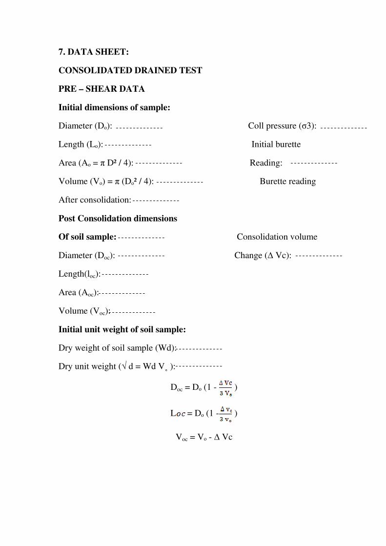
7. DATA SHEET:
CONSOLIDATED DRAINED TEST
PRE – SHEAR DATA
Initial dimensions of sample:
Coll pressure (σ3): Diameter (Dₒ):
Initial burette Length (Lₒ):
Reading: Area (Aₒ = π D² / 4):
Burette reading Volume (Vₒ) = π (Dₒ² / 4):
After consolidation:
Post Consolidation dimensions
Consolidation volume Of soil sample:
Change (∆ Vc): Diameter (Doc):
Length(loc):
Area (Aoc):
Volume (Voc):
Initial unit weight of soil sample:
Dry weight of soil sample (Wd):
Dry unit weight (√ d = Wd V˳ ):
Doc = Dₒ (1 - )
L = Dₒ (1 - )
Voc = Vₒ - ∆ Vc

CONSOL DAYED DFAINED TEST
SHEAR DATA
Cell pressure (σ3) proving ring no
dial gaugeProving ring reading While free lc of
vertical
Diameter of ram (Dr) lc of proving ring DGi
Rate of displacement
13
- V
olu
met
ric
stra
in
%
12
- σ1
/ σ
3
11
- A
xia
l st
ress
σ 1
10
- D
evia
tor
stre
ss σ
1
– σ
3
9-
Dev
iato
r lo
ad P
d
8-
Axia
l lo
ad P
a
7-
Co
rrec
ted
are
a A
1
6-
Volu
me
load
∆ v
5-
Axia
l st
rain
ϵ1
4-
Ver
t . dis
pla
cem
ent
∆ L
3-
pro
vin
g r
ing
d. g
.
2-
Ver
tica
l dia
l g
aug
e
1.B
ure
tte
read
ing
