laboratory flotation testing

ABSTRACT

The properties of the ore have a significant impact on the ultimate gradeand recovery achievable in a flotation circuit. To maximise recovery, theproportion of particles containing the valuable mineral which are floatableshould be maximised. To maximise the grade, the flotation rate of thevaluable mineral should be significantly higher than the flotation rates ofthe gangue minerals in the ore. This is often referred to as ‘maximisingthe selectivity’.

Laboratory batch flotation, in which a 1 - 2 kg sample of ore is floatedusing a standard set of operating conditions, is the standard technique used toassess ore floatability. Traditionally these tests have been performedextensively to determine the ultimate flotation design, screen potentialreagents, determine optimum feed grind size and predict the change inperformance of different ore types. These tests have usually been performedusing the feed ore sample to the process but they are increasingly being usedto characterise the floatability of internal flotation circuit streams and ‘map’how the floatability is changing around a flotation circuit and across differentprocesses.

Key ore floatability parameters (flotation rate constants and proportionof mineral in different floatability classes) can also be derived from thelaboratory test flotation response. The values of these ore floatability

parameters can be evaluated and compared to rank different ore types orreagent suites. These parameters are also suitable for predicting, throughmathematical modelling, the grade-recovery relationship achievable in amultistage flotation circuit.

There are various graphical and modelling techniques that have beendeveloped to interpret laboratory batch flotation test results. In this chapter,the recommended procedure for performing these laboratory flotation testsand the various graphical and modelling analysis methods used tointerpret these test results will be outlined.

INTRODUCTION

To achieve separation in the flotation process, those particlescontaining the valuable mineral need to float and they need tofloat more quickly than those containing predominantly thegangue minerals. The particle size, degree of liberation of theminerals and the hydrophobicity of the mineral surface will inlarge dictate a mineral’s recovery rate. Grinding and chemicaladdition are weapons in the metallurgist’s armoury used tomodify particle properties for a particular ore type in an attemptto achieve maximum separation.

Flotation Plant Optimisation Spectrum Series 16 155

CHAPTER 9

Laboratory Flotation Testing – An Essential Tool forOre CharacterisationKym Runge

Manager – Flotation Process Technology, Metso Minerals (Australia) Limited, Unit 1, 8 - 10 ChapmanPlace, Eagle Farm Qld 4009. Email: [email protected]

Dr Kym Runge is a mineral processing engineer specialising in flotation circuit analysis using modelling andmeasurement techniques. She currently works for Metso Minerals as a flotation specialist both consulting toindustry and managing the development of Metso’s flotation related product line. Her expertise in flotationwas developed during a ten year period at the Julius Kruttschnitt Mineral Research Centre. During this timeshe initially studied for a PhD in flotation modelling and later worked full time as a researcher andconsultant. She was instrumental in the development of JKSimFloat, which is used extensively in theindustry for flotation circuit modelling and analysis. She also has three years industrial experience fromwhen she worked at Pasminco’s Broken Hill flotation concentrator.

Abstract

Introduction

Batch Laboratory Testing Procedures

Techniques Available for Interpretting Batch Laboratory Flotation Test Results

Areas of Application

Advantages and Limitations of Using Batch Flotation Testing for Circuit Diagnosis

Concluding Remarks

References

Appendix – Worked Examples

A vast array of techniques can be used to predict the optimumgrind size and chemical suite to use for a particular ore.Ultimately, there is always a need for small-scale testing tovalidate the results of these analyses or to explore, screen orprioritise different options. This is where laboratory batchflotation testing and the various techniques that can be used toanalyse these batch test results come in useful. They are relativelyeasy and inexpensive to perform in comparison to detailedliberation or chemical speciation analyses and they go some wayto replicating the process conditions that will be present in thefull-scale processing plant.

The aim of this chapter is to outline how these orecharacterisation tests should be performed and demonstrate thevarious graphical and modelling techniques that can be used tointerpret the results produced from these tests.

BATCH LABORATORY TESTING PROCEDURES

The standard procedure

There are various designs of laboratory-scale flotation cells whichcan be used to perform the laboratory batch flotation tests. Mypreference is to use a bottom driven laboratory cell allowingimpeller speed and air rate adjustment, an example of which isshown in Figure 1. This type of cell, used with a fixed depthscraper to regularly remove the entire froth phase duringconcentrate collection, can produce reproducible test results evenbetween different operators.

A typical test involves washing an ore pulp sample into thelaboratory cell. Make-up water is added to achieve the desiredvolume. The impeller is started and set to the desired speed.Collector and depressant (if required) are then added and anappropriate conditioning time is allowed to elapse. At the instantthe air flowmeter is set to the appropriate air rate, the timing ofthe test commences. The concentrate produced from the cellflows and/or is scraped into trays and at designated time intervalsthe trays are removed and replaced. Water is continually added tothe cell to maintain the desired froth level. The test continuesuntil the froth is barren and no more particles are reporting to thefroth in significant quantities. It is recommended that one moreconcentrate be collected after this point to ensure the end point ofthe test can be established.

All concentrate samples and the final tailing sample areweighed wet and dry and assayed for the elements of interest.These results are used to calculate the rate of mineral recovery as

a function of time, usually on a cumulative basis. A typicalcumulative mineral recovery curve is depicted on Figure 2.

As an aside, the water in the concentrate versus the water in theflotation cell will be used to estimate recovery by the entrainmentmechanism. Thus known quantities (or no) water should be usedto wash concentrate into the tray.

Samples to be tested can be collected directly from an operatingflotation circuit, referred to as ‘hot samples’, or prepared in thelaboratory – grinding to produce the appropriate particle size oradding reagent to achieve the required pulp chemistry. The timebetween sample collection and flotation should be minimised toprevent ageing or oxidation of particle surfaces prior to testing.

The weight or size of sample added to the laboratory flotationtest should be chosen to achieve the required pulp density. Pulpdensity is a variable which often affects batch flotation testresults. As it is easier to add water (rather than remove it), it isrecommended that all samples be floated at a low per cent solids(ie less than ten per cent solids). The use of a low per cent solidalso minimises the risk of bubble saturation or overloading. Intests where there is a high proportion of floatable solidsperformed using a low air rate and at a high pulp density, bubblesurfaces can become saturated, resulting in low recovery rates.This condition should be avoided as the result is no longer afunction of only the ore but the air rate used in the test.

The water used to dilute the samples and added during a test tomaintain froth depth should be as similar to that used (or to beused) in the plant as possible. Water properties (ie ph, Eh,temperature, dissolved oxygen and dissolved molecules) willaffect the composition of reagent and deposition products onparticle surfaces, which ultimately affects ore floatability. Frother(as long as it has no collecting properties) should also be added toall make-up water in sufficient quantities to maintain a constantbubble size in the pulp and minimise bubble breakage within thefroth phase. For most frothers, a concentration of 20 ppm withinthe make-up water will be sufficient for this purpose. Distinctadditions of frother in the middle of a test should be avoided asthey can result in a spike in flotation recovery.

It is important that all tests are performed using the same airrate, impeller speed, froth depth and froth scraping rate so thatany change in a batch test result is a consequence of a change inthe ore characteristics rather than to any change in theenvironment in which it is floated. The air rate chosen shouldbe high to prevent bubble saturation and maintain a fluidnon-collapsing froth. Air rates of 10 - 18 L/min are usuallyappropriate for tests performed using a 5 L cell. Impeller speedshould be sufficient to keep all solids in suspension but not thathigh that molecules loosely deposited on surfaces are stripped off.An impeller speed within 750 to 1000 rev/min is recommended.

156 Spectrum Series 16 Flotation Plant Optimisation

CHAPTER 9 – LABORATORY FLOTATION TESTING – AN ESSENTIAL TOOL FOR ORE CHARACTERISATION

FIG 1 - A bottom driven laboratory flotation cell supplied byRunge Engineering.

0

20

40

60

80

100

0 2 4 6 8 10 12 14

Time (min)

Min

era

lR

ec

ov

ery

(%)

FIG 2 - Typical mineral versus recovery time curve obtained from alaboratory batch test.

Ideally the froth should be removed the instant it is formed sothat differences in results can be attributed to changes in pulpflotation kinetics rather than to any change in the flotation frothcharacteristics. As a practical compromise, it is recommendedthat two to three centimetres of froth be maintained throughoutthe test and a scraper of sufficient depth be used to remove allbut 0.5 cm of this froth at regular time intervals. Make-up watershould be added regularly to maintain a constant froth depth assolids and water report to concentrate. A fast froth scraping rate isdesirable but one stroke every ten seconds is usually a speed thatallows the execution of other tasks (addition of water andchanging of trays).

The time intervals over which each concentrate is collectedshould be chosen such that the shape of the mineral recovery timecurves can be well established for the particular operatingconditions chosen to do the tests. A test of a slow floatingplatinum ore, for instance, may require 45 minutes to an hour toreach completion and thus the first concentrate can be collectedafter two minutes of flotation. A faster floating copper porphyryflotation test, however, may finish in five minutes and a firstconcentrate may need to be collected after 20 seconds.

Depending on one’s circumstances, some deviation may berequired from the recommended test conditions (eg use of highper cent solids to obtain sufficient concentrate samples for assay,samples left to sit for long periods). Tests should be performedto establish whether any adverse effect arises from theproposed change.

Refloatation and lock cycle tests

The grade versus recovery relationship derived from a standardbatch laboratory flotation test will not be that achievable in amultiple stage flotation circuit. Multiple stage flotation resultsin a more efficient separation between particles of differentfloatability. Figure 3 demonstrates this point by showing theflotation separation curves for a batch flotation test (calculatedusing flotation modelling techniques) performed over differenttime periods and for tests in which the concentrate has beenrefloated. The flotation separation curve is a plot of recoveryversus the flotation rate of a particle in a particular flotationprocess. If a flotation process was a perfect separator, theseparation curve would be a vertical line – complete recovery ofparticles to the right of the line and no recovery of particles to theleft. The probabilistic nature of the flotation process, however,results in non-ideal separation.

It is clear from these graphs that a change in flotation time(Figure 3a) simply increases or decreases flotation recovery butdoes not result in changes in separation efficiency. A steepeningof the separation curve, however, results from refloating theconcentrate (Figure 3b). This occurs because of the increase inthe fast to slow ratio of particles in the feed to subsequent stages.The net result of this improvement in separation efficiency is animprovement in the concentrate grade or purity achievable at aparticular mineral recovery.

Lock cycle batch flotation experiments provide a better insightinto the expected grade and recovery achievable from multistageprocessing of an ore. These tests are performed such that theyreplicate, on small scale, the full-scale flow sheet. To incorporatethe effect of recycle streams, they are often performed multipletimes with the recycled streams from a previous test added at theappropriate place in the subsequent test. Tests are performed untilthe mass flow in all samples converges to a constant value.Figure 4 shows a schematic of a lock cycle test performed toreplicate a rougher/cleaner flotation circuit in which the cleanertail is recirculated back to the feed.



0

10

20

30

40

50

60

70

80

90

100

0.001 0.01 0.1 1 10

Flotation Rate (min-1)

Re

co

ve

ry(%

)

4

16

8

(a)

0

10

20

30

40

50

60

70

80

90

100

0.001 0.01 0.1 1 10

Flotation Rate (min-1)

Re

co

ve

ry(%

)

Refloatation

(b)

FIG 3 - Recovery of particles with different flotation rates (a) after four, eight and 16 minutes of flotation and (b) after one, two and threerefloatation stages of eight minutes in duration.

Circuit Concentrate

Circuit Tailing

New Feed

New Feed

New Feed

Recycled Tail

Recycled Tail

New Feed

New Feed

New Feed

Recycled Tail

Recycled Tail

New Feed

New Feed

New Feed

Recycled Tail

Recycled Tail

Circuit Concentrate

Circuit Tailing

FIG 4 - Lock cycle test schematic.

The disadvantage of these types of tests is that they are time-consuming to perform and they result in a single grade andrecovery value rather than the relationship between the twovalues derived from the single stage test. To investigate analternative flow sheet or a change in the residence time of a stage,another experiment needs to be performed.

A more time- effective option for estimating multistage circuitgrade and recovery is to model the data from a single stageexperiment (or a lock cycle test). This model can be used tomathematically predict circuit grade and recovery achievablefrom different circuits. The procedures to perform this type ofanalysis will be outlined later in the chapter.

TECHNIQUES AVAILABLE FOR INTERPRETINGBATCH LABORATORY FLOTATION TEST

RESULTS

Mineral recovery, grade versus recovery andselectivity curves

Mineral recovery, grade/recovery and selectivity curves are allgraphs that can be constructed from the information collectedduring a single batch flotation experiment. These curves are idealfor comparing the results of different tests.

The mineral recovery curve displays the cumulative mass ofmineral (on a percentage basis) recovered at each time intervalduring a test. The slope of this curve is an indicator of the rate offlotation recovery and the recovery value at which the curveasymptotes is an indicator of the proportion of floatable mineralin the tested sample (Figure 5).

It is desirable that the valuable mineral in a sample exhibit fastflotation kinetics (steep slope) and the proportion of non-floatingmineral in the sample be minimised. The proportion ofnon-floating valuable mineral is an indicator of the amount ofmineral that is either in particles too large or small for flotation,locked with non-floating particles or with a hydrophilic surfacedue to insufficient collector coverage or depressant coatings.Regardless of the reason, non-floating mineral is not recoverablein a flotation circuit and should be minimised if circuit recoveryis to be maximised.

Flotation is a separation process and thus it’s important that thevaluable mineral is not only recoverable but that it’s recoverableto a greater extent than the gangue mineral. Selectivity curves areideal for this type of evaluation. On these curves, the recovery ofthe valuable mineral is plotted against the recovery of a mineralof interest (Figure 6).

The 45 degree line on this plot represents the points at whichno selectivity occurs – the recovery of valuable mineral is equalto the gangue mineral recovery and no separation is achievable.The further to the right of this line the selectivity curve lies, thebetter. Different selectivity curves should be created for each ofthe gangue minerals of interest as different minerals often exhibitdifferent degrees of selectivity with the valuable mineral.

The overall measure of selectivity in the batch flotation testis the grade (or purity) of the concentrate produced. Thecumulative concentrate grade versus cumulative recovery curves(Figure 7) produced from different tests can be compared todetermine those conditions which result in the best selectivitywith respect to all minerals.

These curves do not, however, give an estimate of the gradeand recovery achievable in a multiple stage flotation circuit. Lockcycle tests or modelling are better suited to this task. Thesecurves do give a good relative measure of selectivity. Animprovement in selectivity in these tests should result in a bettergrade at a particular recovery at full scale.

Entrainment assessment techniques

Gangue can report to the concentrate either attached to bubbles(due to its own hydrophobicity or because of an association witha hydrophobic mineral) or entrained with the water phase. It isimportant to be able to differentiate between these two recoverymechanisms as ultimately this distinction may affect the strategythat is adopted to reduce gangue recovery. This section outlinestechniques that can be used to estimate the degree of entrainmentin a laboratory batch flotation test.



0

20

40

60

80

100

0 2 4 6 8 10 12 14

Time (min)

Min

era

lR

ec

ov

ery

(%)

Increasing Flotation Rate

Increasing Proportion of

Floatable Mineral

FIG 5 - Cumulative mineral recovery curve with the importantfeatures denoted.

0

20

40

60

80

100

0 20 40 60 80 100

Valuable Mineral Recovery (%)

Gan

gu

eM

inera

lR

eco

very

(%)

Increasing Selectivity

FIG 6 - Mineral selectivity curves with the important featuresdenoted.

0

20

40

60

80

100

0 5 10 15 20

Cumulative Concentrate Grade (%)

Cu

mu

lati

ve

Re

co

ve

ryto

Co

nc

en

tra

te(%

)

Improving Overall Selectivity

FIG 7 - Cumulative recovery versus cumulative concentrate gradeproduced during a batch flotation experiment.

Entrainment is a consequence of particles suspended in thepulp phase following the water into the froth and ultimately intothe concentrate. The mass of a mineral entrained into theconcentrate is proportional to the water flow to concentrateand can be estimated using Equation 1 (Johnson, 2005). Theclassification function (Cf,i) is a factor to account for the degree ofdrainage with respect to the water flow and must be estimated toperform the calculation. It is known to fall between zero and one;zero representing the condition of total drainage where there is noentrained recovery of particles regardless of the water recovered,and one representing the condition where there is no drainage andthe concentration of particles in the water in the concentrate (dueto entrainment) is the same as in the pulp phase. Cf,i is known tobe strongly dependent on size with the coarser particlesexhibiting a high degree of drainage (Cf,i = 0) and the fineparticles usually following the water phase (Cf,i = 1).

F C Fi f, i i, pulp w= ω (1)

where:

Fi is the flow of a component i into the concentrate due toentrainment

Cf,i is the classification function for component i

ωi,pulp is the mass to water ratio of component i in the pulpphase

Fw is the flow of water to the concentrate

Thus to calculate the recovery by entrainment in a batch test,the water to solids ratio in the pulp, water flow to concentrate andan estimate of Cf,i is required. The water flow to concentrate canbe measured and the average water to solids ratio in each stagecan be estimated based on knowledge of the cell volume and theparticle mass balance. The challenge is to estimate the degree ofdrainage in the system.

If one of the minerals is known to be non-floating, an inversionof Equation 1 can be used to calculate a Cf,i estimate for the otherminerals in the ore. This, unfortunately, is not usually the casewith even the non-floating minerals locked to some extent withthe valuable and exhibiting floatability. Johnson (2005) publishedtypical values of Cf,i for siliceous non-sulfide gangue (Table 1).These values coupled with knowledge of the particle sizedistribution of a particular sample can enable a reasonableestimate of Cf,i to be calculated.

Alternatively, Cf,i can be estimated using results from the batchtest by recognising that towards the end of an experiment, thepredominant particle recovery mechanism is entrainment. If onecalculates the ratio of mineral to water in both the concentrateand pulp and plots this value for each stage of a batch experiment(Figure 8), it usually decreases, asymptoting at a particular valuetowards the end of the test. This value is an estimate of the Cf,i

value. The larger values at the beginning are because recovery isdue to entrainment and flotation in these earlier stages.

Once a Cf,i estimate has been obtained and the gangueentrainment flow has been calculated (Equation 1), a cumulativeentrainment recovery curve can be constructed which can be

compared to the overall recovery curve for that mineral(Figure 9). The difference in these two curves is the proportion ofthe mineral recovered due to true flotation (attachment tobubbles).

Ore floatability mapping in a flotation circuit

Traditionally batch flotation tests have only been performed usingsamples representative of a flotation circuit feed. Much can belearnt, however, by floating the samples collected from differentstreams of an operating flotation circuit.

During flotation the faster floating particles will report to theconcentrate streams, whereas the slower floating particles willreport predominantly to the tailing streams. This results indifferent streams possessing very different ore floatabilityproperties. As an example, Figure 10 shows the copper recoveryachieved in batch flotation tests performed using different streamsfrom Rio Tinto’s Northparkes flotation circuit.

This information can then be assessed in terms of mineralrecovery and selectivity. A traditional rule of thumb is torecirculate streams to a point of similar assay. A better philosophyis to recirculate streams to a point of similar floatability.

The final tailing is of special importance as it is discardedand any valuable mineral contained in this stream is a lostopportunity. High valuable mineral recovery rates coupled withgood selectivity in a tailing stream batch test is an indication ofinsufficient residence time in the circuit.



Size fractions (μm)

-11 -16 +11 -23 +16 -33 +23 -44 +33

0.77 0.46 0.30 0.24 0.13

TABLE 1Typical values of Cf,i (after Johnson, 2005).

0.0

0.5

1.0

1.5

2.0

2.5

0 5 10 15

Time (min)

Ra

tio

Cf,i Estimate

Maximum C Limit

Gangue to Water Ratio in Pulp

Gangue to Water Ratio in ConcentrateRatio

f,i

FIG 8 - Cf,i calculated using Equation 1 versus time in a batchflotation test.

0

10

20

30

40

50

60

70

0 5 10 15

Time (min)

Gan

gu

eR

eco

very

(%)

Overall

EntrainmentEstimate

FIG 9 - Curves used to assess the predominant gangue recoverymechanism in a batch flotation test.

Streams with poor valuable mineral to gangue mineralselectivity are appropriate targets for regrinding or depressant orcollector addition. Batch flotation of different streams in aflotation circuit enables the appropriate streams for this type ofmodification to be delineated from those that would not benefitfrom this type of processing.

Regular batch laboratory flotation test mapping during circuitsurveys will provide a record of ore floatability properties –enabling the comparison of this property between different surveys.

Nodal analysis comparisons

The nodal analysis technique was developed to compare thefloatability of particles before and after processes (ie nodes)within a flotation circuit (Runge et al, 1997). It involvescomparing the mineral recovery rate and selectivity achieved inbatch laboratory flotation tests of the feed and product streams ofa node. A node is defined as a point in a circuit where streams areeither combined, separated or altered in some way (Figure 11). Anode can be a single unit such as a flotation cell, a regrind mill ora pump sump, a combination of units (eg a bank of cells) or evenan entire circuit with the feed being split into the final concentrateand final tailing stream.

The experimental feed and product mineral recovery rates ormineral selectivity curves derived from laboratory batch flotationtests can be compared directly when there is only one feed streamand one product stream from a node.

This direct comparison is difficult, however, when there aremultiple feed or product streams. In many cases it is alsoimpossible to obtain ‘the desired’ samples from the flotationprocess. In these cases, the mineral recovery rate of a ‘combinedfeed’ or ‘combined product’ stream can be estimated bymathematically combining the experimental results of thestandard laboratory batch flotation tests on two or more streams(Equation 2) based on their relative flows in the circuit.

R =F

Mineral jCombined Stream, t minutes

Mineral jStream s

Mineral jStream s, t minutes

s = 1

n

Mineral

R

F

×∑

jStream s

s

n

=∑

1

(2)

where:

FMineral jStream s is the flow rate of mineral j in stream s

RMineral jStream s, t minutes is the cumulative recovery of mineral j in stream

s after t minutes of flotation in the standardlaboratory batch flotation test

Take for example a flotation column. A column has a singlefeed but two product streams. Equation 2 can be used torecombine the concentrate and tailing stream to produce a single‘combined’ product stream result. The combined streamfloatability can then be compared to the feed stream floatabilityto assess whether there has been any change across the unit.Figure 12 shows the galena recovery rate measured in a batchflotation test of the feed, concentrate and tailing streams of anindustrial column. It also shows the calculated ‘combinedproduct’ stream which, in this case, is very similar to the columnfeed. It can therefore be concluded that floatability does notchange significantly across this unit. The difference in galenarecovery rates in the concentrate and tailing stream is attributed tothe faster floating galena-containing particles concentrating in theconcentrate streams and the slower floating galena-containingparticles concentrating in the tailing streams. Using this techniquein a number of different flotation circuit operations, it has beenshown that ore floatability is not often affected in a full-scaleflotation cell (Runge et al, 2006).

Regrinding and reagent addition are employed in a flotationcircuit specifically to alter particle floatability. Often theeffectiveness of these processes is assessed by expensive andoften inconclusive on-off testing. Comparison of ore floatabilityusing nodal analysis techniques can enable a direct assessment ofthe effectiveness of these particle modification operations. InFigure 13a for example, it is obvious that staged reagent additionhas resulted in a significant increase in the proportion of floatablecopper in the circuit. In Figure 13b it is obvious that regrinding



0

20

40

60

80

100

0 2 4 6 8

Time (min)

Co

pp

er

Re

co

ve

ry(%

)

Rougher Feed

Rougher Con

Rougher Tail

Scavenger Con

Scavenger Tail

Cleaner Feed

Cleaner Con

Cleaner Tail

Recleaner Feed

Recleaner Con

Recleaner Tail

Clnr Scav Tail

FIG 10 - Copper recoveries achieved in the batch tests performedon different streams in the Northparkes flotation circuit.

(a) (b)

(d)(c)

FIG 11 - Examples of nodes in a flotation circuit. (a) Flotation cell;(b) tower mill; (c) pump sump; (d) flotation circuit.

0

10

20

30

40

50

60

70

80

90

100

0 10 20 30 40

Time (min)

Ga

len

aR

ec

ov

ery

(%)

Column Feed

Column Con

Column Tail

Column Con +

Column Tail

FIG 12 - Galena recovery versus time for the feed, concentrate,tailing and combined product of an industrial-scale flotation

column (after Runge et al, 1997).

has not resulted in an improvement in the chalcopyrite/pyriteselectivity. These types of observations provide the metallurgistwith invaluable information regarding the effect of an oremodification process.

These techniques will be demonstrated in a worked exampleincluded at the end of this chapter. For a more detailed example,the reader is referred to Runge, Franzidis and Manlapig, 2004 inwhich these techniques are used to assess the effect of stagedreagent addition, regrinding and lime addition on ore floatabilityin an industrial circuit.

Ore parameter estimation techniques

The mineral recovery response measured in a laboratory batchflotation experiment can be used to calculate ore floatabilityparameters – numbers which represent the rate and extent towhich a mineral will float. These parameters can be used as ameans of comparison of different batch test experiments or withina flotation model for performance prediction.

Flotation is considered a first order kinetic process, recoverybeing a function of the time in the process (t) and a flotation rateconstant (k). In a batch laboratory flotation environment, recoverycan be calculated using Equation 3.

R t= − −1 exp( )k (3)

The flotation rate constant is a function of the operatingconditions in the cell and also the size, mineralogy and surfacechemical speciation of the particles being floated. There are anumber of different types of particles in an ore sample and eachwill float with a different flotation rate – thus an ore sampleexhibits a distribution of floatabilities. There are no methodscurrently available for measuring each particle’s individual rate.Instead the problem is simplified by assuming the form of thefloatability distribution. The two methods most commonly usedinvolve assuming a continuous shape for the distribution (egrectangular distribution (Klimpel, 1980)) or splitting a mineralinto different floatability components. In this chapter, derivationand use of multiple component parameters will be discussed. Forthose wanting more information regarding shaped distributions, thereader is referred to a paper written by Chander and Polat (1994).

Mineral recovery in a batch flotation test using multiplecomponents can be calculated using Equation 4.

R m t))ii= 1

n

i= − −∑ ( exp(1 k (4)

The rate of each component (ki) and the proportion of themineral in that class (mi) are the ore floatability parameters of thesystem that can be derived from batch laboratory flotation test data.This involves calculating the ‘best’ set of these parameters thatminimise the sum of squares difference between the recoveriescalculated using Equation 4 and that measured in the laboratorybatch flotation experiments. This difference can, optionally,be weighted by the standard deviation of the experimentaldata (Equation 5). These problems are easily set up on anExcel spreadsheet using the Solver add-in to performthe minimisation.

SSER R )

SDj.calculated j.experimental

2

j.experiment

=−(

al2

j∑ (5)

The number of components that can be derived to describe amineral’s floatability is dependent on the amount of dataavailable to do the parameter estimation. Unfortunately the datafrom a single batch laboratory flotation test is only sufficient todetermine, with statistical confidence, the parameters associatedwith a simple representation of the system (one floating and onenon-floating component). More complex representation requiresan increase in the experimental data set size.

Harris (1998) recognised that this data set size could beincreased by using information collected from laboratory batchflotation tests performed using different streams of a circuit.A circuit by its very nature results in a redistribution ofthe floatability components – fast floatability componentspredominantly reporting to the concentrate streams and the slowerand non-floating components predominantly reporting to thetailing streams. If we assume that the feed consists of a number offloatability components, the other streams are also made up ofthese same floatability components, just in a different ratio.Analysis involves assuming the rate of each floatabilitycomponent in the different batch tests is the same and that themass of each floatability component is conserved across differentnodes in the process. These constraints enable the data toparameter ratio to be significantly increased and enableparameters of multicomponent systems to be derived withstatistical confidence. The measured distribution of floatabilitycomponents in the different streams of an industrial flotationcircuit derived using this type of analysis is shown in Figure 14.

In a similar vein, laboratory batch flotation tests can beperformed with multiple stages or with recycle streams toincrease the number of datapoints available for parameter



0

20

40

60

80

100

0 2 4 6 8 10

Time (min)

Ch

alc

op

yri

teR

eco

very

(%)

Feed to Reagent Node

Product of Reagent Node

(a)

0

20

40

60

80

100

0 20 40 60 80 100

Chalcopyrite Recovery (%)

Py

rite

Re

co

ve

ry(%

) Combined Feed

Product

(b)

FIG 13 - Nodal analysis comparative graphs: (a) mineral recovery before and after collector addition, (b) chalcopyrite/pyrite selectivitybefore and after regrinding.

estimation. Thus multiple ore floatability parameter estimationcan be performed without the need to collect samples from anoperating flotation circuit.

A step by step worked example of the ore parameter derivationtechnique will be provided at the end of this chapter.

Comparison of ore floatability parameters

Ore floatability parameters provide the metallurgist with numbersthat can be used to quantitatively assess and compare thefloatability of ore in different laboratory batch flotation tests.

For optimal separability in a flotation circuit, the valuablemineral flotation rate should be high and the proportion of slowor non-floating valuable mineral should be minimised. Gangueflotation rates should ideally be low and a large proportion of thegangue mineral should be non-floatable. It will not be possible toseparate mineral components of similar flotation rate so the ratioof the slow floating gangue to slow floating valuable mineralflotation rate is also an important parameter.

Hay and Rule (2003) characterised the ore floatability of theore feeding a number of different platinum concentrators using atwo floating component model. They found that the concentraterecovery and grade were strongly correlated with the fraction offast floating valuable mineral with a proportion of the slowfloating fraction being recoverable when the ratio of the slowvaluable mineral to gangue flotation rate ratio was above athreshold value.

Ore floatability component mapping, as illustrated in Figure 14,can be used in conjunction with the mineral recovery andselectivity graphical information to assess the appropriatedestination of recycle streams and the target streams forregrinding, collector or depressant addition.

Simulation using ore floatability parameters

The advantage of ore floatability parameters over the traditionalgraphical techniques, are that they can be used for prediction.Once determined, they can be used to rapidly investigate many

circuit scenarios. They can replace the need for complex lockcycle tests, giving estimates of the ultimate grade and recoveryachievable in multistage flotation.

The aim of simulation is to calculate the distribution offloatability components across a proposed circuit. Beginning withthe feed and the first unit in the circuit, recovery in the productstreams are calculated. This calculation sequence is continued foreach unit process, the product of earlier processes forming thefeed to subsequent processes. Recycle streams during the firstiteration are set to zero and multiple iterations of circuitcalculations are performed until the mass in these recycle streamsconverges to a constant value. Once convergence has beenachieved, the mass of the different floatability components ofeach mineral in each stream can be added together. These mineralmasses can be used to calculate stream mineral grade (mineralmass divided by total mass in stream) and recovery (mass withrespect to feed).

At each process in the circuit, recovery equations are used tocalculate product component flows. Wherever streams are mixed,for instance, the mass of each floatability component in theproduct stream is equal to the addition of the mass of this samefloatability component in the feed streams.

The recovery equation used for a flotation process is dependenton its particle residence time distribution. For a semi-batchprocess (like that performed in the laboratory batch flotation test)recovery of each component is calculated using Equation 3.Conventional mechanical cells behave as perfect mixers and thushave a different recovery equation (Equation 6).

Rk

1 + k= τ

τ(6)

The flotation recovery equation can be extended to includeparameters associated with entrainment and the cell operatingvariables (eg air rate, froth depth). Flotation cell water recoveryequations are also required to calculate the circuit water flowinformation required for cell residence time calculations. For



88.9

5.8

5.3

11.7

2.7

0.0

3.8

4.2

5.3

3.8

3.7

5.3

85.1

2.1

0.0

2.5

0.5

0.0

11.7

2.2

0.0

80.7

1.8

0.0

6.9

0.3

0.0

1.3

3.7

5.3

0.0

0.5

0.0

4.8

1.9

0.0

Legend

Fast Floating

Slow Floating

Non Floating

FIG 14 - Mass in different copper floatability components around the Northparkes industrial flotation circuit (based on 100 units ofcopper in the feed).

more information on these types of simulations and the methodsrequired to determine the parameters of these relationships, thereader is referred to Harris et al, 2002.

A simplification to these more complex models can be used toassess the separability of a particular ore in a particular flowsheet. The effect of the cell operating variables and residencetime can be lumped into a single parameter, the cell operatingconstant, θ (Loveday, 1966). Flotation recovery of a componentis a function of only this parameter and its particular batchflotation test rate constant (Equation 7).

Rk

1 + kbatch

batch

= θ

θ(7)

Multiple simulations are performed for a particular flow sheet,with the cell operating constants, θ, randomised in each stage.This randomisation is a representation of the range of differentcell volumes/cell operating conditions which could be used toachieve flotation separation. It is equivalent to the flotationoperator slowing or speeding up the process to achieve thedesired concentrate grade and recovery at each stage.

The resulting final concentrate grade/recovery numbers fromthese simulations can be plotted. Figure 15 shows examples of thetype of curves generated using this type of analysis. These curveswere generated using ore floatability constants derived frombatch laboratory experiments applied to a three stage flotationcircuit. The result is not a single grade versus recoveryrelationship, as changes in the cell operating constant in one stageresult in both a change in recovery but also a change in theseparation efficiency of the circuit.

These curves can be generated to compare the floatability ofdifferent ore types (Figure 15b) or to compare the ability ofdifferent flow sheets to separate the minerals in a particular oresample (Figure 16).

Simulations required to create these curves can be performedon an Excel spreadsheet. Alternatively, packages such asJKSimFloat and Limn© have been designed to enable thesetypes of simulations to be performed rapidly in a userfriendly environment.

Estimation of full-scale residence timerequirements

The time it takes for a mineral to be recovered in a batch laboratoryflotation test can be used to estimate the cell volume and thenumber of cells at full scale required to achieve this same recovery.Recovery rates in the batch cell environment are usually

significantly higher than those measured at full scale due to thehigher degree of turbulence and the higher froth recoveriesachievable at small scale. A scale-up factor (C) can be introducedto the full-scale recovery equation to account for these differencesand relate full-scale recovery to the rate measured in a batchlaboratory flotation test (kbatch) (Equation 8).

RC

1 + Cbatch

batch

= k

k

τ

τ(8)

The cell scale-up factor is a complex function of the operatingconditions at full scale and those used in the batch laboratoryflotation test. It will also be strongly dependent on the ore and itseffect on the full-scale froth characteristics. It is the author’srecommendation that this scale-up factor be determined bycomparing batch and full-scale kinetics in an existing concentratorprocessing a similar ore. The use of globally quoted scale-upfactors (eg batch test rate is twice the rate at full scale) is notrecommended as this factor changes significantly with theoperating conditions used in both the batch test and full-scale cells.

Once the batch test ore floatability parameters and the scale-upfactor have been established, simulations can be performed todetermine the number of cells at a particular volume that arerequired to achieve the desired bank recovery. Additionalcapacity is usually factored into this analysis to account for anyerror and the usual increase in capacity (over design) oftendemanded from a flotation circuit over time.



40

42

44

46

48

50

52

54

56

40 50 60 70 80 90 100

Circuit Recovery (%)

Fin

alC

on

ce

ntr

ate

Gra

de

(%)

40

42

44

46

48

50

52

54

56

40 50 60 70 80 90 100


Fin

alC

on

ce

ntr

ate

Gra

de

(%)

(a) (b)

FIG 15 - Circuit grade and recovery simulated in a three stage flotation circuit. (a) For a particular ore type, (b) for the same ore subject todifferent reagent/regrinding schemes.

40

42

44

46

48

50

52

54

56

58

60

40 60 80 100


Fin

alC

on

cen

trate

Gra

de

(%)

Three Stage

Four Stage

FIG 16 - Circuit grade and recovery simulated for the same oreprocessed in a three and four stage flotation circuit.

AREAS OF APPLICATION

Laboratory batch flotation testing can be used as a diagnostic toolthroughout the development and life of a flotation circuit.

Even before a project has commenced, batch laboratoryflotation of drill core samples provide the information required tomake decisions regarding a project’s viability. Throughout thedevelopment of a flotation circuit flow sheet, batch tests are usedto screen and determine the appropriate reagent suite and dosagerates, the target grind size and an estimate of the circuit residencetime requirements.

From the day a flotation circuit is commissioned, themetallurgist strives to better understand the process andimplement changes which will improve or optimise operation.Batch laboratory flotation testing is one of a suite of tools used inthis process. New reagents are almost always screened first inthese small tests before implementation at full scale.

After implementation of a change in grind size, reagent or circuitchange at industrial scale, batch flotation tests can be used to assessthe effect of the change on mineral recovery rates and selectivity.

The ore feeding a flotation circuit is continually changing asrock is extracted from different areas of the mine. Batch testing isa valuable tool for comparing the floatability of different ores orpredicting the metallurgical performance that will be achievedwhen a particular ore is processed.

Flotation modelling techniques published in the literature(Harris et al, 2002; Runge et al, 2001; Coleman, Urtubia andAlexander, 2006) are using batch testing to determine orecharacterisation properties. These models can be used forflotation circuit design, flotation circuit diagnosis and simulationof alternative operating strategies. They enable an estimation ofthe overall change in grade and recovery achievable in aparticular process fed an ore with a particular mineral selectivity.

In summary, laboratory batch flotation testing is an essentialtool, which when used appropriately, helps a metallurgist todesign new flotation processes, develop strategies for improvinga flotation circuit and ultimately assess the effectiveness ofthese strategies.

ADVANTAGES AND LIMITATIONS OF USINGBATCH FLOTATION TESTING FOR CIRCUIT

DIAGNOSIS

Small-scale batch laboratory tests are relatively cheap and easy toperform. Almost all concentrator laboratories are equipped withlaboratory flotation cells and the associated equipment requiredto prepare and process the samples produced from a test. Theyalso have the advantage that, to a significant degree, theyreplicate the flotation process that occurs at full scale.

Batch tests also have the advantage that they enable the orefloatability to be analysed in isolation to those effects related tocircuit operation. Poor flotation recovery measured in a circuitsurvey can be due to a number of different effects: poor orefloatability, insufficient residence time, use of overly deep frothdepths, to name a few. Batch laboratory tests are usuallyperformed using the same operating conditions and thus anychange between tests can be attributed solely to a difference inore floatability. Batch tests performed in conjunction with circuitsurveys can help decouple ore floatability and circuit operationeffects and highlight the cause of flotation recovery loss.

What is often forgotten when analysing batch flotation testresults, however, is that they are a good measure of pulpfloatability but sometimes a poor indicator of full-scale frothphase performance. The froth in a small-scale laboratory test isonly a couple of centimetres in depth and is continually removed.

In a full-scale cell the froth can be ten to 50 cm in depth and thereare usually significant transportation distances between a point onthe surface of the froth and the nearest launder. The frothproduced in a small-scale cell is often very different in bubblesize, texture and viscosity to that observed when the same ore isprocessed at full scale. This can result in a particular reagentsuite, producing a superior pulp floatability (and thus batch testresult) but poor recovery in a full-scale cell because of its effecton movement of the froth phase.

The primary assumption associated with batch laboratory testanalysis is that pulp selectivity in the small scale is similar towhat would be achieved in the full-scale flotation machine. It’slikely this is a valid assumption in mechanical cells but lesslikely in alternative flotation technologies. The low degree ofturbulence in a column, for instance, usually results in the poorrecovery of coarse particles which are recovered quickly in abatch flotation test.

Another risk during batch laboratory flotation testing is theremoval of loosely deposited surface coatings. The higheragitation energies which exist in a small-scale cell can sometimesremove molecules which would remain in situ in the full-scaleflotation environment.

These limitations, as with most diagnostic techniques, meanthat those conclusions drawn from batch laboratory testing shouldbe verified through full-scale trials.

Much can be gained by performing batch laboratory flotationtests in conjunction with other measurements. Batch laboratoryflotation tests indicate the overall result of a change. Sizing,mineralogical and chemical analysis tools can be used todetermine the reason for a particular result, often suggestingalternative batch laboratory experiments to trial.

CONCLUDING REMARKS

In this chapter, batch laboratory testing procedures and themodelling and graphical techniques that can be used to analysethe results of these tests have been reviewed.

It has been demonstrated that batch laboratory flotation testshave a role to play throughout the lifetime of a particular flotationcircuit operation. They can be used during the design of newflotation processes to develop strategies for improving a flotationcircuit and, ultimately, to assess the effectiveness of these strategies.

They have the advantage that they are relatively cheap and easyto perform and to an extent, replicate the full-scale flotationprocess. They enable an assessment of ore floatability without thecomplication of changing cell operating variable effects. Effects,due to differences between the small-scale and full-scale cell,should be kept in mind when interpreting results.

The value of laboratory batch flotation testing is greatlyenhanced when performed in parallel with other techniques thatcan assist with data interpretation.

REFERENCESChander, S and Polat, M, 1994. In quest of a more realistic flotation

kinetics model, in Proceedings IV Meeting of the SouthernHemisphere on Mineral Technology and III Latin American Congresson Froth Flotation (eds: S Castro and J Alvarez), pp 481-500.

Coleman, R G, Urtubia, H E and Alexander, D J, 2006. A comparison ofBHP Billiton’s Minera Escondida flotation concentrators, inProceedings 38th Annual Meeting of the Canadian MineralProcessors, pp 349-370 (Canadian Institute of Mining, Metallurgyand Petroleum: Montreal).

Harris, M C, 1998. The use of flotation plant data to simulate flotationcircuits, in Proceedings SAIMM Mineral Processing DesignSchool (Southern African Institute of Mining and Metallurgy:Johannesburg).



Harris, M C, Runge, K C, Whiten, W J and Morrison, R D, 2002.JKSimFloat as a practical tool for flotation process design andoptimization, in Mineral Processing Plant Design, Practice andControl, vol 1, pp 461-478 (Society for Mining, Metallurgy, andExploration: Littleton).

Hay, M P and Rule, C M, 2003. Supasim: A flotation plant design andanalysis methodology, Minerals Engineering, 16(11):1103-1109.

Johnson, N W, 2005. A review of the entrainment mechanism and itsmodelling in industrial flotation processes, in Proceedings Centenaryof Flotation Symposium (ed: G J Jameson), pp 487-496 (TheAustralasian Institute of Mining and Metallurgy: Melbourne).

Klimpel, R R, 1980. Selection of chemical reagents for flotation, in MineralProcessing Plant Design, Ch 45, pp 907-934 (The American Institute ofMining, Metallurgical, and Petroleum Engineers: Littleton).

Loveday, B K, 1966. Analysis of froth flotation kinetics, Trans IMM,75:C219-C225.

Runge, K C, Dunglison, M E, Manlapig, E V and Franzidis, J-P, 2001.Floatability component modelling – A powerful tool for flotationcircuit diagnosis, in Proceedings Fourth International Symposium onFundamentals of Minerals Processing, pp 93-107 (Canadian Instituteof Mining, Metallurgy and Petroleum: Montreal).

Runge, K C, Franzidis, J P and Manlapig, E V, 2004. Optimisation offlotation pulp selectivity utilising nodal analysis, in Proceedings 36thAnnual Meeting of the Canadian Mineral Processors, pp 575-597(Canadian Institute of Mining, Metallurgy and Petroleum: Montreal).

Runge, K C, Harris, M C, Franzidis, J P and Manlapig, E V, 2006.Conservation of floatability across processes in industrial flotationcircuits, in Proceedings XXIII International Mineral ProcessingCongress (eds: G Onal, N Acarkan, et al), vol 3, pp 1909-1914(Promed Advertising Agency).

Runge, K C, Harris, M C, Frew, J A and Manlapig, E V, 1997. Floatabilityof streams around the Comino Red Dog lead cleaning circuit, inProceedings Sixth Annual Mill Operators’ Conference, pp 157-163(The Australasian Institute of Mining and Metallurgy: Melbourne).

APPENDIXWORKED EXAMPLES

Example 1 – regrind evaluation

A tower mill has been incorporated into the Eureka lead circuitto regrind lead rougher concentrate in an effort to improveliberation and thus the grade achievable in the lead flotationcircuit concentrate.

Batch laboratory flotation tests were performed on the rougherconcentrate and the reground rougher concentrate (after reagentaddition) to assess whether this unit is having the desired effect.

Six timed concentrates and a tailing sample were producedfrom each test. Table A1 outlines the mineral grade measured ineach of these samples.

This data was then used to calculate the cumulative grade andrecovery achieved as a function of time in these tests. Figure A1shows the grade versus recovery curve and Figure A2 shows thegalena gangue selectivity curves.

In contrary to what was expected, regrinding has not resulted inan improvement in the floatability of the ore. At low galenarecoveries, the grade recovery relationship is significantly poorerin the ‘after regrinding’ batch test. At high galena recoveries, therelationship in the two tests is very similar.

This result is primarily due to deterioration in the pyrite-galenaselectivity. Galena recovery rate has changed very little by theregrinding process, whereas there has been a significant increasein pyrite recovery (Figure A3). There is very little difference inthe galena-sphalerite selectivity and a marginal improvement ingalena-gangue selectivity.

The grinding environment often results in changes in thecondition of particle surfaces – iron hydroxide coatings, forinstance, can deposit on all surfaces during grinding with mildsteel balls. Some change is occurring to the pyrite particles in thisgrinding system, resulting in an increased recovery rate. Surfacechemical speciation of particle surfaces before and after grindingwould almost certainly explain the reason for this observed resultand maybe suggest strategies to reverse the effect.

Under the current chemical conditions, however, regrinding oflead concentrate should be discontinued.

Example 2 – circuit survey comparison usingnodal analysis

Lime is used periodically in the zinc cleaner scavenger flow sheet(Figure A4) of the Eureka concentrate to depress pyrite. Debatereigns as to whether this lime results in an improvement inperformance. To try and resolve the dispute between thoseadvocating lime addition and those against it, two circuit surveysof the zinc cleaner scavenger flow sheet were performed – onewith lime on and one with lime off. Batch laboratory tests wereperformed to measure the floatability of the feed, concentrate and



Sample Time(min)

Before regrinding After regrinding

Galena Sphalerite Pyrite NSG Galena Sphalerite Pyrite NSG

Concentrate 1 0 - 0.5 76.71 14.08 4.02 5.20 72.80 14.86 6.77 5.58

Concentrate 2 0.5 - 1.5 68.66 20.80 5.73 4.81 68.54 17.67 7.66 6.13

Concentrate 3 1.5 - 4 48.42 31.44 9.12 11.03 57.27 25.34 9.52 7.87

Concentrate 4 4 - 8 25.88 45.83 16.35 11.95 28.29 44.10 15.60 12.00

Concentrate 5 8 - 12 18.17 50.83 21.40 9.60 15.99 50.99 19.02 14.01

Concentrate 6 12 - 20 12.54 51.77 23.49 12.21 12.19 50.05 20.80 16.96

Tailing 4.72 53.02 21.25 21.01 5.75 45.20 22.84 26.21

TABLE A1Mineral grade of samples produced from batch flotation testing of a lead concentrate before and after grinding.

0

20

40

60

80

100

40 50 60 70 80

Galena Grade (%)

Ga

len

aR

ec

ov

ery

(%)

Rougher Concentrate

Reground Rougher

Concentrate

FIG A1 - Galena grade versus recovery achieved in batch flotationtests of the lead rougher concentrate before and after regrinding.

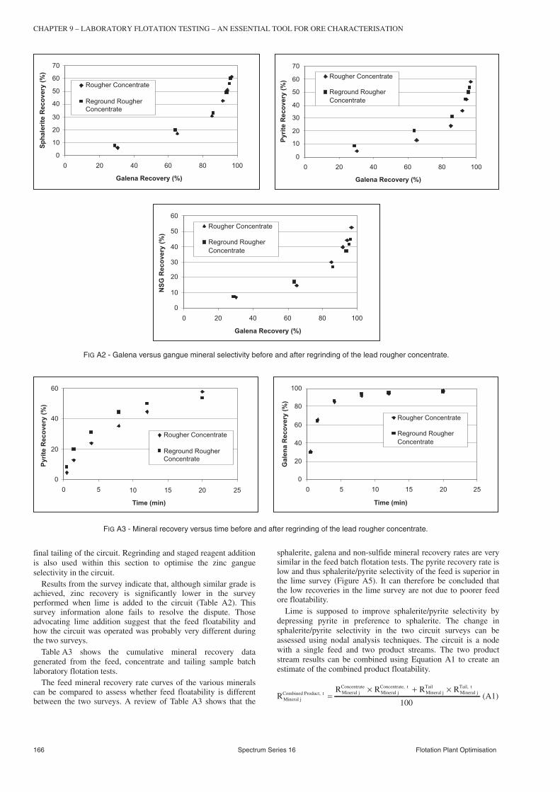
final tailing of the circuit. Regrinding and staged reagent additionis also used within this section to optimise the zinc gangueselectivity in the circuit.

Results from the survey indicate that, although similar grade isachieved, zinc recovery is significantly lower in the surveyperformed when lime is added to the circuit (Table A2). Thissurvey information alone fails to resolve the dispute. Thoseadvocating lime addition suggest that the feed floatability andhow the circuit was operated was probably very different duringthe two surveys.

Table A3 shows the cumulative mineral recovery datagenerated from the feed, concentrate and tailing sample batchlaboratory flotation tests.

The feed mineral recovery rate curves of the various mineralscan be compared to assess whether feed floatability is differentbetween the two surveys. A review of Table A3 shows that the

sphalerite, galena and non-sulfide mineral recovery rates are verysimilar in the feed batch flotation tests. The pyrite recovery rate islow and thus sphalerite/pyrite selectivity of the feed is superior inthe lime survey (Figure A5). It can therefore be concluded thatthe low recoveries in the lime survey are not due to poorer feedore floatability.

Lime is supposed to improve sphalerite/pyrite selectivity bydepressing pyrite in preference to sphalerite. The change insphalerite/pyrite selectivity in the two circuit surveys can beassessed using nodal analysis techniques. The circuit is a nodewith a single feed and two product streams. The two productstream results can be combined using Equation A1 to create anestimate of the combined product floatability.

RR

Mineral jCombined Product, t Mineral j

Concentrat

=e

Mineral jConcentrate, t

Mineral jTail

MineraR R R× + × l jTail, t

100(A1)



0

10

20

30

40

50

60

70

0 20 40 60 80 100

Galena Recovery (%)

Sp

ha

leri

teR

ec

ov

ery

(%)

Rougher Concentrate

Reground Rougher

Concentrate

0

10

20

30

40

50

60

70

0 20 40 60 80 100

Galena Recovery (%)

Py

rite

Re

co

ve

ry(%

)

Rougher Concentrate

Reground Rougher

Concentrate

0

10

20

30

40

50

60

0 20 40 60 80 100

Galena Recovery (%)

NS

GR

ec

ov

ery

(%)

Rougher Concentrate

Reground Rougher

Concentrate

FIG A2 - Galena versus gangue mineral selectivity before and after regrinding of the lead rougher concentrate.

0

20

40

60

0 5 10 15 20 25

Time (min)

Py

rite

Re

co

ve

ry(%

)

Rougher Concentrate

Reground Rougher

Concentrate

0

20

40

60

80

100

0 5 10 15 20 25

Time (min)

Ga

len

aR

ec

ov

ery

(%)

Rougher Concentrate

Reground Rougher

Concentrate

FIG A3 - Mineral recovery versus time before and after regrinding of the lead rougher concentrate.

where:

RMineral jConcentrate is the recovery of mineral j to concentrate

RMineral jTail is the recovery to tailing of mineral j

RMineral jCombined Product, t is the cumulative recovery of mineral j in the

combined product after t minutes of flotation

The results of this calculation are shown in Table A4.Once the combined product floatability has been calculated, feed

and product mineral recoveries can be compared. Figure A6 shows

the sphalerite/pyrite selectivity in the feed and product streams ofthis particular circuit. Sphalerite/pyrite selectivity in the surveywhen lime is not added, improves dramatically across the circuit. Itcan therefore be concluded that regrinding and the reagent additionduring this survey have had a positive effect on the ability toseparate sphalerite and pyrite. In contrast, sphalerite, pyriteselectivity deteriorates in the survey in which lime is added.

This deterioration in sphalerite/pyrite selectivity is due to adecrease in the sphalerite recovery rate (in contrast to an increasewhen lime is not added to the circuit) and a small but similardecrease in the recovery of pyrite (Figure A7).

Use of nodal analysis in this example has shown that limeaddition in the circuit does not result in appreciable improvementsin sphalerite/pyrite selectivity. The deterioration in valuable togangue mineral selectivity will have had a significant impact onthe ability to separate minerals in this circuit. Adjustments incircuit operation would have occurred to maintain grade but at acost of losing zinc recovery.

As a confirmation of this conclusion, nodal analysis was alsoperformed before and after lime addition in this circuit (Rungeet al, 2004). These tests show that lime addition dramaticallydecreases the floatability of all minerals, but sphaleritein particular.

It thus can be concluded that lime addition is clearly not thesolution to improving pyrite/selectivity in this circuit. Batchlaboratory testing performed in conjunction with survey workenabled a more definitive analysis of circuit operation.



To Final Tail

Sump

To Final Concentrate

Sump

Stage 2

Regrind

Stage 1

Cleaning Columns

Activator

Collector

Activator Collector

Lime

To Final Tail

Sump

To Final Concentrate

Sump

Stage 2

Regrind

Stage 1

Cleaning Columns

Activator

Collector

Activator Collector

Lime

FIG A4 - Eureka zinc cleaner scavenging circuit.

0

20

40

60

80

100

40 50 60 70 80 90 100

Sphalerite Recovery (%)

Py

rite

Re

co

ve

ry(%

) Survey - No Lime Added

Survey - Lime Added

FIG A5 - Sphalerite/pyrite selectivity measured in the feed batchtests performed during the two circuit surveys.

Details of survey Concentrate grade (%) Recovery to concentrate (%)


No lime added 6.2 79.7 7.0 7.2 57.8 86.2 11.4 5.5

Lime added 5.0 79.0 8.0 8.0 33.0 61.5 8.4 4.2

TABLE A2Metallurgical performance achieved during each survey.

Example 3 – ore floatability parameter modellingof laboratory batch test data

There is a concern that a future ore to be fed to the Eurekaconcentrator will be more difficult to treat in the lead circuit thanthe current ore. Liberation analysis has indicated it has a morecomplex lead mineralogy.

A multiple stage batch laboratory flotation test was performedusing the future ore to enable its ore floatability parameters to bedetermined and compared to those of the current ore. Grind sizeand reagent dosage rates were similar to those used in the plant.The test involved floating a sample of the future ore for eight

minutes with two samples of concentrate collected – one from thefirst two minutes (denoted rougher concentrate) and one from thetwo to eight minute time period (denoted scavenger concentrate).The rougher concentrate was then refloated in a cleaner stagewhere concentrates were collected from zero to 20 seconds, 20 to40 seconds, 40 to 60 seconds and from one to two minutes. Thescavenger concentrate was then combined with the tailing fromthe cleaner stage and refloated in a cleaner scavenger stage for sixminutes. Concentrates were collected from zero to 0.5 minutes,0.5 to one minute, one to two minutes and two to six minutes. Adiagram depicting the stages of the test and samples produced isshown in Figure A8.



Cumulative time(min)

Mineral cumulative recovery in feed batch test

No lime addition Lime addition


0.33 22.5 33.3 10.8 7.5 23.2 36.4 9.7 10.3

1 49.9 63.4 28.2 19.8 49.0 66.6 22.2 21.8

2 66.8 79.1 43.3 29.9 65.7 80.7 33.5 31.8

4 82.4 89.2 58.0 40.9 79.3 90.4 48.3 42.0

8 89.5 94.3 69.6 51.1 87.7 94.8 62.1 52.2

12 92.4 96.1 75.5 57.6 91.2 96.5 69.7 58.9


Mineral cumulative recovery in concentrate batch test



0.33 32.2 37.5 18.9 16.6 19.3 22.9 15.0 16.6

1 68.6 74.9 42.1 38.2 46.8 53.8 37.7 36.9

2 86.0 90.4 59.3 52.7 65.2 73.2 52.5 52.3

4 94.7 97.3 76.2 68.7 80.4 87.8 67.6 67.7

8 98.0 99.1 89.0 81.1 91.1 96.0 81.5 83.0

12 98.7 99.5 91.8 83.8 94.6 98.0 87.4 88.5


Mineral cumulative recovery in tailing batch test



0.33 13.5 24.2 8.4 6.2 13.8 18.7 7.6 5.9

1 31.7 53.0 23.0 11.6 33.9 41.2 19.0 13.8

2 46.8 68.4 35.9 17.5 49.5 56.0 29.9 20.0

4 61.0 77.1 48.1 25.7 62.9 67.0 40.7 25.7

8 73.0 84.1 62.6 35.0 75.2 75.9 53.8 34.2

12 77.4 86.0 67.2 40.1 80.2 79.3 60.6 39.7

TABLE A3Cumulative mineral recovery achieved in the feed, concentrate and tailing batch tests performed during the two circuit surveys.


Mineral cumulative recovery in combined product



0.33 24.3 35.7 9.6 6.8 15.6 21.2 8.2 6.3

1 53.0 71.9 25.2 13.1 38.2 49.0 20.6 14.7

2 69.5 87.4 38.6 19.4 54.7 66.6 31.8 21.4

4 80.5 94.5 51.3 28.1 68.7 79.8 43.0 27.5

8 87.4 97.0 65.6 37.5 80.4 88.2 56.2 36.3

12 89.7 97.6 70.0 42.5 85.0 90.8 62.9 41.8

TABLE A4Cumulative mineral recovery of the combined product streams from the two circuit surveys.

The samples produced from the test were dried and weighedand analysed for lead content – the results of which are shown inTable A5.

It is decided to represent the ore floatability of the system bythree lead components (fast, slow and non-floating lead) andthree gangue components (fast, slow and non-floating gangue).Three components are the maximum number that could bederived with confidence from the experimental data available.Gangue is a term to refer to the weight in each sample that is‘not lead’. To determine the flotation rate and proportion of leadand gangue in each of the floatability components, an Excelspreadsheet was set up to calculate the weight and assay of theexperimental samples based on a flotation model. Solver, anadd-in tool to Excel, was then used to determine the orefloatability parameters that minimise the difference between themeasured and calculated sample information.

Table A6, Table A7 and Table A8 show the calculation tablesthat were set up in Excel to perform the calculations.

Table A9 shows the calculation of the weight of lead in eachbatch test sample based on any set of lead floatability parameters.

The calculation is performed in three tables. The first tablecontains the parameters to be derived from the fitting exercise.The values first input into the table are an estimate. Note that therate and mass fraction of the non-floating component are notfitted parameters. The rate of the non-floating component is zeroand the proportion of material in the non-floating component isone minus the fraction in the other components.

The second table calculates the recovery of each component ineach stage of the batch test (Rs). Recovery is a function of theflotation rate of the component (ki) and the time of flotation (t)(Equation A2).

R 1 exp ts = − −( )ki (A2)



Survey - No Lime Added

0

20

40

60

80

100

40 50 60 70 80 90 100


Py

rite

Re

co

ve

ry(%

)

Feed

Combined Product

Survey - Lime Added

0

20

40

60

80

100

40 50 60 70 80 90 100


Py

rite

Re

co

ve

ry(%

)

Feed

Combined Product

FIG A6 - Sphalerite/pyrite selectivity measured in the feed and product of the two circuit surveys.

0

20

40

60

80

100

0 5 10 15

Time (min)

Sp

ha

leri

teR

ec

ov

ery

(%)

Feed No Lime

Feed Lime

Product No Lime

Product Lime

0

20

40

60

80

100

0 5 10 15

Time (min)

Py

rite

Re

co

ve

ry(%

)

Feed No Lime

Feed Lime

Product No Lime

Product Lime

FIG A7 - Sphalerite and pyrite recovery rates measured in the feed and product of the two circuit surveys.

Rougher

(2 minutes)

Scavenger

(6 minutes)New Feed

Clner Scav

(6 minutes)

Concentrates

Tailing

Cleaner

Tailing

Rougher

(2 minutes)

Scavenger

(6 minutes)

Clner Scav

(6 minutes)

Cleaner

(2 minutes)

Cleaner

(2 minutes)

FIG A8 - Representation of multiple stage batch laboratory flotationtest – samples produced denoted by a red circle.

Sample Solids(g)

% Lead % Gangue

Cleaner concentrate 1 13.4 75.9 24.1




Cleaner scavenger concentrate 1 9.2 55.8 44.2




Cleaner scavenger tailing 19.6 7.2 92.8

Tailing 2096.7 0.9 99.1

Recalculated feed 2200.0 3.1 96.9

TABLE A5Multiple stage batch test results.

In the final table, the weight of each component in each batchtest sample throughout the duration of the test is calculated. Theweight in each component in the test feed is established bymultiplying the total weight of lead in the feed (an input) by theproportion of lead in each component as specified in the firsttable. The weight in the concentrate of each stage is determinedby multiplying the weight in the feed to the stage by the stagerecovery (Rs). The weight in the tail of each stage is the feedminus the concentrate weight. These calculations are performed

in sequence, with either the concentrate or tailing (or both in thecase of the cleaner scavenger feed) of previous stages becomingthe feed to subsequent stages.

The total weight of lead reporting to each concentrate or tailingstream in the batch test is then calculated by summing theweights of its floatability components.

The identical calculation sequence is performed to determinethe mass of gangue in each of the batch test samples according toa set of gangue specific floatability components (Table A7).



Parameter table Fast Slow Non

Lead flotation rates (min-1) 0.932 0.201 0.000

Proportion of lead in feed in each component 0.642 0.099 0.258

Stage recovery matrix Time (min) Calculated recovery in stage

Fast Slow Non

Rougher 2 84.5% 33.1% 0.0%

Scavenger 6 99.6% 70.1% 0.0%

Cleaner 1 0.333 26.7% 6.5% 0.0%

Cleaner 2 0.333 26.7% 6.5% 0.0%

Cleaner 3 0.333 26.7% 6.5% 0.0%

Cleaner 4 1 60.6% 18.2% 0.0%

Cleaner scavenger 1 0.5 37.3% 9.6% 0.0%


Cleaner scavenger 3 1 60.6% 18.2% 0.0%


Component distribution matrix Weight of component in sample

Batch test sample Fast Slow Non Total

Feed 43.84 6.78 17.64 68.26

Rougher concentrate 37.05 2.25 0.00 39.29

Scavenger concentrate 6.77 3.18 0.00 9.95

Tailing 0.03 1.35 17.64 19.02

Cleaner feed (rougher concentrate) 37.05 2.25 0.00 39.29

Cleaner concentrate 1 9.89 0.15 0.00 10.03




Cleaner tail 5.75 1.50 0.00 7.25

Cleaner scavenger feed (SC + CT) 12.51 4.68 0.00 17.19

Cleaner scavenger concentrate 1 4.66 0.45 0.00 5.11




Cleaner scavenger tailing 0.05 1.40 0.00 1.44

Combined cleaner concentrate 31.30 0.74 0.00 32.05

Combined cleaner scavenger concentrate 12.47 3.28 0.00 15.75

Total concentrate 43.77 4.03 0.00 47.79

Total tailings 0.07 2.75 17.64 20.47

TABLE A6Lead flotation model Excel spreadsheet.

The weight of lead and gangue calculated in each stream can beused to calculate the total weight of solids and the lead and gangueassay of each batch test sample. This calculated assay is thencompared to the actual assay measured during the test (Table A8).

To calculate the total sum of squares error associated with thesystem, the error of each experimental datapoint must be estimated.For this exercise, the Whiten function is used to estimate thestandard deviation of the assays (Equation A3) and a relative errorof 2.5 per cent is used as the error of the solid weights.

SD 1 if assay 9%

SD assay / 10 0.1 if assay 9%

= >= + <

(A3)

The squared error associated with each experimental datapointis calculated using Equation (A4). The total sum of squares erroris the sum of the squared errors.

SEd d

SDcalculated experimental

experimental2=

−( )2

(A4)



Parameter table Fast Slow Non

Gangue flotation rates 0.654 0.099 0.000

Proportion of gangue in feed in each component 0.009 0.030 0.961

Stage recovery matrix Time (min) Calculated recovery in stage

Fast Slow Non

Rougher 2 73.0% 17.9% 0.0%

Scavenger 6 98.0% 44.7% 0.0%

Cleaner 1 0.333 19.6% 3.2% 0.0%

Cleaner 2 0.333 19.6% 3.2% 0.0%

Cleaner 3 0.333 19.6% 3.2% 0.0%

Cleaner 4 1 48.0% 9.4% 0.0%





Component distribution matrix Weight of component in sample

Batch test sample Fast Slow Non Total

Feed 19.70 63.15 2050.89 2133.74

Rougher concentrate 14.37 11.32 0.00 25.70

Scavenger concentrate 5.22 23.18 0.00 28.40

Tailing 0.11 28.65 2050.89 2079.65

Cleaner feed (rougher concentrate) 14.37 11.32 0.00 25.70





Cleaner tail 3.89 9.29 0.00 13.18

Cleaner scavenger feed (SC + CT) 9.11 32.47 0.00 41.58





Cleaner scavenger tailing 0.18 17.95 0.00 18.13

Combined cleaner concentrate 10.49 2.03 0.00 12.51

Combined cleaner scavenger concentrate 8.93 14.52 0.00 23.45

Total concentrate 19.42 16.55 0.00 35.96

Total tailings 0.29 46.60 2050.89 2097.78

TABLE A7Gangue flotation model Excel spreadsheet.

Once the spreadsheet has been set up in the way describedabove, Solver (an add-in tool in Excel) can be used to determinethe lead and gangue parameters which minimise the total sum ofsquares error. For this example, Solver is able to find a set ofparameters which result in a good fit to the experimental data.

In Table A9, the parameters derived from the analysis aboveare compared to those derived from a similar test performed usingthe ore currently processed by the plant.

The flotation rates of the different components in the twodifferent ores are similar. The ore does have poorer floatingcharacteristics than the current ore. The proportion of floatablelead is significantly lower and the proportion of floatable ganguehas increased. This is an indication that the future ore is lessliberated at the grind size tested.

The flotation model that was developed to determine the oreparameters can also be used to simulate various different batchtest configurations – predicting the change in grade and recoverythat would be produced if the test was run in a different way.

To use the model, the parameters of the ore are input into theparameter table and the time of each stage is input into thestage recovery matrix. The lead grade and lead recovery ofthe combined concentrate (cleaner and cleaner scavengerconcentrate) is calculated by the model. Using the parametersderived for the current ore and the future ore, the model was usedto predict the combined concentrate lead grade and recoveriesthat would be achieved if different times were used in the variousstages of the batch test. Table A10 show the different simulationsthat were performed and the results. Figure A9 shows a graphicalcomparison of the results derived for the two ores.



Calculated data Experimental data Standard deviation Squared error

Batch test sample Assay Solids(g)

Assay Solids(g)

Assay Solids(g)

Assay Solids(g)Lead Gangue Lead Gangue Lead Gangue Lead Gangue

Feed 3.10 96.90 2202.00

Rougher concentrate 60.46 39.54 64.99

Scavenger concentrate 25.94 74.06 38.34

Tailing 0.91 99.09 2098.67 0.85 99.13 2096.7 0.19 1.00 52.4 0.09 0.00 0.00

Cleaner feed (rougher concentrate) 60.46 39.54 64.99

Cleaner concentrate 1 75.94 24.06 13.21 76.7 24.09 13.4 1.00 1.00 0.3 0.58 0.00 0.22




Cleaner tail 35.48 64.52 20.43

Cleaner scavenger feed (SC + CT) 29.25 70.75 58.77

Cleaner scavenger concentrate 1 55.45 44.55 9.22 58.3 44.16 9.2 1.00 1.00 0.2 8.10 0.15 0.03




Cleaner scavenger tailing 7.38 92.62 19.57 7.5 92.79 19.6 0.82 1.00 0.5 0.02 0.03 0.00

Combined cleaner concentrate 71.92 28.08 44.56

Combined cleaner scavengerconcentrate

40.18 59.82 39.20

Total concentrate 57.06 42.94 83.76

Total tailings 0.97 99.03 2118.24

Sum of squares error 21.52

TABLE A8Calculation of the sum of squares error associated with the model fit.

Parameter Future ore Current ore

Fast Slow Non Fast Slow Non

Lead flotation rates 0.93 0.20 0.0 0.99 0.16 0.0

Proportion of lead in each component in feed 0.64 0.10 0.26 0.71 0.08 0.21

Gangue flotation rates 0.65 0.10 0.0 0.62 0.07 0.0

Proportion of gangue in each component in feed 0.009 0.03 0.96 0.007 0.02 0.97

TABLE A9Stage batch test ore floatability results.

The ore floatability of the future ore, as measured in the batchflotation test, is clearly poorer than that currently treated. Thelead recovery achievable at a particular grade is ten per cent lowerin the future ore simulations than in the current ore simulations.Increased recoveries may be possible at a finer grind. Additionaltest work would be required to substantiate this hypothesis.



Model simulation Batch test stage time Future ore Current ore

Rougher Scavenger Cleaner Cleanerscavenger

Lead grade Leadrecovery

Lead grade Leadrecovery

Base case 2.00 6.00 2.00 6.00 57.06 70.02 70.44 74.72

Simulation 1 2.00 6.00 0.50 1.50 66.69 55.63 77.69 61.67

Simulation 2 4.00 12.00 2.00 6.00 52.54 71.41 66.97 75.92

Simulation 3 6.00 18.00 2.00 6.00 50.52 71.78 65.05 76.32

Simulation 4 12.00 24.00 2.00 6.00 48.91 72.04 63.26 76.61

Simulation 5 12.00 24.00 4.00 12.00 43.01 73.71 57.32 78.28

Simulation 6 12.00 24.00 1.00 3.00 55.64 68.08 69.04 73.31

Simulation 7 6.00 18.00 1.00 3.00 57.03 67.83 70.34 73.08

Simulation 8 2.00 6.00 1.00 3.00 62.21 66.21 74.16 71.71

Simulation 9 2.00 6.00 0.50 1.50 66.69 55.63 77.69 61.67

Simulation 10 1.00 3.00 0.50 1.50 69.76 52.34 79.80 58.69

Simulation 11 1.00 3.00 1.00 3.00 66.11 62.97 76.87 69.06

Simulation 12 1.00 3.00 2.00 6.00 62.02 66.60 73.98 72.02

TABLE A10Multiple stage batch test simulation results.

0

10

20

30

40

50

60

70

80

90

0 20 40 60 80 100

Lead Grade (%)

Le

ad

Re

co

ve

ry(%

)

Future Ore

Current Ore

FIG A9 - Simulated batch test lead grade and recovery of thefuture and current ore.