laboratory course in physical chemistry for fundamental studies · 2019-04-09 · molarity,...
TRANSCRIPT

CHAIR OF PHYSICAL CHEMISTRY
TECHNISCHE UNIVERSITÄT MÜNCHEN
Laboratory Course in Physical Chemistry
for Fundamental Studies
Experiments Manual
The reproduction of this manual is funded by the tuition grant
of the Chemistry Faculty


_
© 2016 Chairs of Physical Chemistry of the Technical University of Munich
8th Edition (8th April 2019).
Editing, typing and printing: Michele Piana, Karin Stecher, Alexander Ogrodnik, Sonja Uhl, Matthias Stecher and
Peter Kämmerer.
Chair of Technical Electrochemistry and Second Chair of Physical Chemistry
Alle Rechte vorbehalten. Die Vervielfältigung auch einzelner Teile, Texte oder Bilder – mit Ausnahme der in SS 53,
54 UrhG ausdrücklich genannten Sonderfälle – gestattet das Urheberrecht nur, wenn sie mit den Lehrstühlen oder
dem Praktikumsleiter vorher vereinbart wurde.

i
Table of Contents 1 Vapour-Pressure Curve and Boiling-Point Elevation ............................................................................... 1
1.1 Context and aim of the experiment ....................................................................................................... 1
1.1.1 Important concepts to know ......................................................................................................... 1
1.1.2 Most common questions to be answered .................................................................................... 1
1.1.3 Further preparations before the experiment ................................................................................. 1
1.2 Theory .................................................................................................................................................... 2
1.2.1 Phase diagrams ............................................................................................................................ 2
1.2.2 Vapour pressure ............................................................................................................................ 2
1.2.3 Colligative properties and boiling-point elevation ......................................................................... 3
1.3 Experimental details and evaluation ...................................................................................................... 5
1.3.1 Experimental execution................................................................................................................. 5
1.3.2 Data evaluation ............................................................................................................................. 7
1.4 Applications of the experiment and its theory ....................................................................................... 8
1.5 Appendixes ............................................................................................................................................ 8
1.5.1 Derivation of the boiling-point elevation from the chemical potential ........................................... 8
1.5.2 Basic instructions to use the software .......................................................................................... 9
1.6 Literature.............................................................................................................................................. 11
2 Freezing-Point Depression ....................................................................................................................... 12
2.1 Context and aim of the experiment ..................................................................................................... 12
2.1.1 Important concepts to know ....................................................................................................... 12
2.1.2 Most common questions to be answered .................................................................................. 12
2.1.3 Further preparations before the experiment ............................................................................... 12
2.2 Theory .................................................................................................................................................. 13
2.2.1 Phase diagrams .......................................................................................................................... 13
2.2.2 Colligative properties .................................................................................................................. 13
2.2.3 Derivation of freezing-point depression from chemical potential................................................ 13
2.2.4 Supercooling of a liquid .............................................................................................................. 15
2.3 Experimental details and evaluation .................................................................................................... 15
2.3.1 Experimental execution............................................................................................................... 15
2.3.2 Data evaluation ........................................................................................................................... 17
2.4 Applications of the experiment and its theory ..................................................................................... 17
2.5 Appendixes .......................................................................................................................................... 17
2.5.1 Basic Instructions to use the software ........................................................................................ 17
2.6 Literature.............................................................................................................................................. 19
3 Joule-Thomson Effect .............................................................................................................................. 20
3.1 Context and aim of the experiment ..................................................................................................... 20
Table of Contents
ii
3.1.1 Important concepts to know ....................................................................................................... 20
3.1.2 Most common questions to be answered ................................................................................... 20
3.1.3 Further preparations before the experiment ............................................................................... 20
3.2 Theory ................................................................................................................................................. 21
3.2.1 Internal energy and intermolecular interactions .......................................................................... 21
3.2.2 The Joule-Thomson-Experiment ................................................................................................. 22
3.2.3 Thermodynamic analysis of the Joule-Thomson effect............................................................... 22
3.2.4 Derivation of the expansion coefficient and the Joule-Thomson coefficient .............................. 25
3.2.5 Calculation of the inversion curve using the van-der-Waals equation of state ........................... 26
3.3 Experimental details and evaluation ................................................................................................... 26
3.3.1 Experimental execution ............................................................................................................... 27
3.3.2 Data evaluation ........................................................................................................................... 28
3.4 Applications of the experiment and its theory .................................................................................... 29
3.5 Appendixes ......................................................................................................................................... 29
3.5.1 Basic instructions to use the software ........................................................................................ 29
3.5.2 Instruction for data treatment ...................................................................................................... 30
3.5.3 Van-der-Waals parameters ......................................................................................................... 32
3.5.4 Further implementations in the derivation of the Joule-Thomson coefficient for real gases ....... 32
3.5.5 Further implementations in the derivation of the inversion temperature for real gases .............. 33
3.5.6 Virial coefficient ........................................................................................................................... 34
3.6 Literature ............................................................................................................................................. 34
4 Combustion Enthalpy via Bomb Calorimetry .......................................................................................... 35
4.1 Context and aim of the experiment..................................................................................................... 35
4.1.1 Important concepts to know ....................................................................................................... 35
4.1.2 Most common questions to be answered ................................................................................... 35
4.1.3 Further preparations before the experiment ............................................................................... 35
4.2 Theory ................................................................................................................................................. 35
4.2.1 Heat transactions, internal energy and reaction enthalpy ........................................................... 36
4.2.2 Combustion reactions ................................................................................................................. 36
4.2.3 Bomb calorimetry ........................................................................................................................ 37
4.3 Experimental details and evaluation ................................................................................................... 38
4.3.1 Experimental execution ............................................................................................................... 38
4.3.2 Data evaluation ........................................................................................................................... 41
4.4 Applications of the experiment and its theory .................................................................................... 41
4.5 Appendixes ......................................................................................................................................... 42
4.5.1 Basic Instructions to use the software ........................................................................................ 42
4.6 Literature ............................................................................................................................................. 44
5 Mixing Enthalpy of Binary Mixtures ......................................................................................................... 45
5.1 Context and aim of the experiment..................................................................................................... 45

Table of Contents
iii
5.1.1 Important concepts to know ....................................................................................................... 45
5.1.2 Most common questions to be answered .................................................................................. 45
5.1.3 Further preparations before the experiment ............................................................................... 45
5.2 Theory .................................................................................................................................................. 45
5.2.1 Partial molar volume ................................................................................................................... 46
5.2.2 Partial molar Gibbs’ energy......................................................................................................... 46
5.2.3 Chemical potential of liquids ....................................................................................................... 46
5.2.4 Liquid mixtures of ideal solutions ............................................................................................... 47
5.2.5 Liquid mixtures of real solutions ................................................................................................. 48
5.2.6 Properties of acetone and water and their interactions .............................................................. 49
5.3 Experimental details and evaluation .................................................................................................... 50
5.3.1 Experimental execution............................................................................................................... 50
5.3.2 Data evaluation ........................................................................................................................... 52
5.4 Applications of the experiment and its theory ..................................................................................... 52
5.5 Appendixes .......................................................................................................................................... 52
5.5.1 Basic instructions to use the software ........................................................................................ 52
5.6 Literature.............................................................................................................................................. 55
6 Equilibrium Thermodynamics .................................................................................................................. 56
6.1 Context and aim of the experiment ..................................................................................................... 56
6.1.1 Important concepts to know ....................................................................................................... 56
6.1.2 Most common questions to be answered .................................................................................. 56
6.1.3 Further preparations before the experiment ............................................................................... 56
6.2 Theory .................................................................................................................................................. 57
6.2.1 Equilibrium thermodynamics ...................................................................................................... 57
6.2.2 Effect of temperature on an equilibrium reaction ........................................................................ 58
6.2.3 Absorption spectroscopy ............................................................................................................ 58
6.2.4 The reaction of Rhodamine B ..................................................................................................... 59
6.3 Experimental details and evaluation .................................................................................................... 60
6.3.1 Experimental execution............................................................................................................... 60
6.3.2 Data evaluation ........................................................................................................................... 63
6.4 Applications of the experiment and its theory ..................................................................................... 64
6.5 Literature.............................................................................................................................................. 64
7 The Electromotive Force and its Dependence on Activity and Temperature ...................................... 65
7.1 Context and aim of the experiment ..................................................................................................... 65
7.1.1 Important concepts to know ....................................................................................................... 65
7.1.2 Most common questions to be answered .................................................................................. 65
7.1.3 Further preparations before the experiment ............................................................................... 65
7.2 Theory .................................................................................................................................................. 66
7.2.1 Activity and concentration .......................................................................................................... 66

Table of Contents
iv
7.2.2 Electrochemical cells and emf .................................................................................................... 67
7.2.3 Thermodynamic Cell Potential and Nernst Equation .................................................................. 68
7.2.4 Half-cell potentials, standard potentials and reference electrodes ............................................. 68
7.2.5 The Daniell cell and its temperature dependence ....................................................................... 70
7.3 Experimental details and evaluation ................................................................................................... 71
7.3.1 Experimental execution ............................................................................................................... 71
7.3.2 Data evaluation ........................................................................................................................... 75
7.4 Applications of the experiment and its theory .................................................................................... 76
7.5 Appendixes ......................................................................................................................................... 76
7.5.1 Basic Instructions to use the Software........................................................................................ 76
7.6 Literature ............................................................................................................................................. 78
8 Activation Energy of a First-Order Reaction ........................................................................................... 79
8.1 Context and aim of the experiment..................................................................................................... 79
8.1.1 Important concepts to know ....................................................................................................... 79
8.1.2 Most common questions to be answered ................................................................................... 79
8.1.3 Further preparations before the experiment ............................................................................... 79
8.2 Theory ................................................................................................................................................. 79
8.2.1 Reaction rate, reaction order and molecularity ........................................................................... 79
8.2.2 Differential equation and time course of an irreversible first-order reaction ............................... 80
8.2.3 Temperature dependence of a reaction rate constant ................................................................ 81
8.2.4 Correlation between activation energy and reaction enthalpy .................................................... 82
8.2.5 Decomposition of the tertiary amylbromide ................................................................................ 82
8.3 Experimental details and evaluation ................................................................................................... 83
8.3.1 Experimental execution ............................................................................................................... 83
8.3.2 Data evaluation ........................................................................................................................... 84
8.4 Applications of the experiment and its theory .................................................................................... 84
8.5 Appendixes ......................................................................................................................................... 84
8.5.1 Basic Instructions to use the Software........................................................................................ 84
8.6 Literature ............................................................................................................................................. 87
9 Kinetics of the Inversion of Sucrose ........................................................................................................ 88
9.1 Context and aim of the experiment..................................................................................................... 88
9.1.1 Important concepts to know ....................................................................................................... 88
9.1.2 Most common questions to be answered ................................................................................... 88
9.1.3 Further preparations before the experiment ............................................................................... 88
9.2 Theory ................................................................................................................................................. 88
9.2.1 Catalytic reactions....................................................................................................................... 88
9.2.2 Kinetics of first-order and pseudo-first-order reactions .............................................................. 89
9.2.3 Polarization of light ...................................................................................................................... 90
9.2.4 Optically active molecules........................................................................................................... 90

Table of Contents
v
9.2.5 Polarimetry .................................................................................................................................. 91
9.2.6 Optical activity and decomposition of sucrose ........................................................................... 91
9.3 Experimental details and evaluation .................................................................................................... 94
9.3.1 Experimental execution............................................................................................................... 94
9.3.2 Data evaluation ........................................................................................................................... 96
9.4 Applications of the experiment and its theory ..................................................................................... 96
9.5 Appendixes .......................................................................................................................................... 96
9.5.1 General acid catalysis ................................................................................................................. 96
9.5.2 Lippich half-shade polarizer ........................................................................................................ 97
9.6 Literature.............................................................................................................................................. 98
10 Primary Kinetic Salt Effect ....................................................................................................................... 99
10.1 Context and aim of the experiment ..................................................................................................... 99
10.1.1 Important concepts to know ....................................................................................................... 99
10.1.2 Most common questions to be answered .................................................................................. 99
10.1.3 Further preparations before the experiment ............................................................................... 99
10.2 Theory .................................................................................................................................................. 99
10.2.1 Activity of ions in solution ........................................................................................................... 99
10.2.2 Hypothesis of the activated complex and effect of ionic strength on reaction kinetics ............ 100
10.2.3 Decomposition of murexide and its reaction rate ..................................................................... 102
10.3 Experimental details and evaluation .................................................................................................. 103
10.3.1 Experimental execution............................................................................................................. 103
10.3.2 Data evaluation ......................................................................................................................... 105
10.4 Applications of the experiment and its theory ................................................................................... 105
10.5 Literature............................................................................................................................................ 105
11 Estimation and Propagation of Measurement Uncertainties .............................................................. 106
11.1 Basics and types of measurement uncertainties ............................................................................... 106
11.1.1 Coarse errors ............................................................................................................................ 106
11.1.2 Statistical errors ........................................................................................................................ 107
11.1.3 Systematic errors ...................................................................................................................... 109
11.1.4 Precision and accuracy ............................................................................................................. 109
11.2 Quantification of the precision of a measurement ............................................................................. 110
11.2.1 Mean value and statistical error ................................................................................................ 110
11.2.2 Probability distribution .............................................................................................................. 111
11.2.3 Gaussian (or normal) distribution .............................................................................................. 113
11.3 Error propagation ............................................................................................................................... 115
11.3.1 Propagation of systematic errors .............................................................................................. 115
11.3.2 Gaussian propagation of statistical errors ................................................................................ 115
11.3.3 Useful rules for Gaussian error propagation ............................................................................. 117
11.3.4 Standard deviation of the mean value ...................................................................................... 119

Table of Contents
vi
11.4 Least square fitting ........................................................................................................................... 119
11.4.1 Residuals ................................................................................................................................... 121
11.4.2 Linearization .............................................................................................................................. 122
11.4.3 Linear regression ....................................................................................................................... 122
11.4.4 Estimation of the errors of the regression parameters .............................................................. 123
11.4.5 Important example .................................................................................................................... 123
11.5 Appendixes ....................................................................................................................................... 125
11.5.1 Function of several independent variables ................................................................................ 125
11.5.2 Standard deviation as a function of the variance ...................................................................... 126
11.5.3 The principle of “maximum likelihood” ...................................................................................... 126
11.5.4 Deriving the errors of the regression parameters ...................................................................... 127
1
1 Vapour-Pressure Curve and Boiling-Point
Elevation
1.1 Context and aim of the experiment
In this experiment, the boiling point of a pure solvent as a function of pressure, i.e., its vapour-pressure curve,
is measured. This is used to determine the vaporization enthalpy, the vaporization entropy and the ebullioscopic
constant of the solvent. Furthermore, an unknown substance is added to the solvent and its molecular weight is
determined from the measured boiling-point elevation [1.1 - 1.5].
1.1.1 Important concepts to know
Colligative properties, chemical potential, phase diagram, boiling point, triple point, critical point, ebullioscopic
constant, vapour pressure, vapour pressure curve, Clausius-Clapeyron equation, enthalpy of vaporization, entropy
of vaporization, ideal and non-ideal solution, non-associating solvent, Raoult’s law, Henry’s law, Gibb’s phase rule,
molarity, molality, superheating of a solution.
1.1.2 Most common questions to be answered
How can you graphically explain the effect of boiling-point elevation using the temperature dependence of
the chemical potential of a solvent and its solution?
Is the boiling-point elevation an enthalpy effect or an entropy effect? Explain your answer.
How can you explain in a simple way the effect of boiling-point elevation concerning the entropy of the
system?
Which characteristic distinguishes the phase diagram of water from those of most other solvents?
In the expression for the ebullioscopic constant, the concentration is given as molality (mol/kg) instead of
molarity (mol/L)? What is the advantage of this?
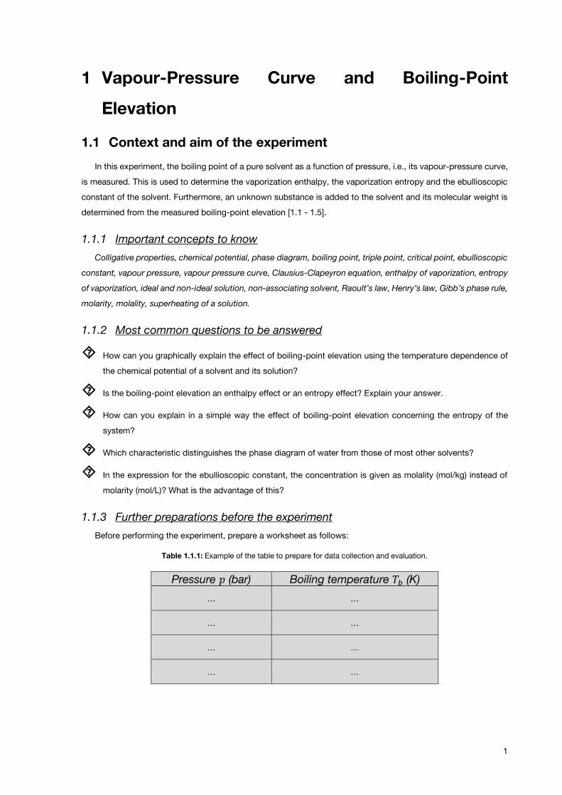
1.1.3 Further preparations before the experiment
Before performing the experiment, prepare a worksheet as follows:
Table 1.1.1: Example of the table to prepare for data collection and evaluation.
Pressure 𝑝 (bar) Boiling temperature 𝑇𝑏 (K)
… …
… …
… …
… …

Vapour-Pressure Curve and Boiling-Point Elevation
2
1.2 Theory
1.2.1 Phase diagrams
The phase diagram of a substance shows the regions of pressure 𝑝 and temperature 𝑇 at which its various
phases (solid, liquid or gas) have the minimum Gibbs free energy and are thus thermodynamically stable at
equilibrium (Figure 1.2.1). The lines separating the regions are called phase boundaries and show the values of 𝑝
and 𝑇 at which two phases coexist in equilibrium.
Figure 1.2.1: Phase diagram of a) water and b) CO2. Phase boundaries are labelled with A, B and C. D and E are the triple point and the critical point, respectively.
The phase diagram describes many important properties of a substance: boiling point, standard boiling point,
freezing point (also called melting point), standard freezing point (also called standard melting point), triple point
and critical point. The student must be familiar with these terms.
Figure 1.2.1 shows that, at the thermodynamic equilibrium an arbitrary number of phases cannot exist
simultaneously. This is stated in the Gibbs’ phase rule, which further allows determination of the maximum
possible degrees of freedom 𝑓 at a certain position of the phase diagram. For liquids this is
𝑓 = 𝑁 − 𝑃 + 2 (1.1)
where 𝑃 is the number of existing phases and 𝑁 is the number of independent kinds of molecules in the system.
The Gibbs’ phase rule is derived from the Gibbs-Duhem equation, which indicates that in a thermodynamic system
not all intensive variables (like temperature, pressure, molar quantities etc.) are changeable independently.
1.2.2 Vapour pressure
Consider a liquid sample of a pure substance in a closed vessel. When the liquid and its vapour are in
equilibrium, the same number of molecules leaves the liquid by vaporization and goes back from the vapour to
the liquid by condensation. Under these conditions, the pressure of the vapour is called the vapour pressure of
the liquid at a certain temperature. The vapour pressure is independent of the presence of other components in
the gas phase, e.g., air. In this case, the partial pressure of the liquid equals its vapour pressure at a certain
temperature. Further heating of the liquid causes an increase in vapour pressure. The temperature at which the
vapour pressure of the liquid equals the external pressure is called boiling point. At this temperature, the
vaporization can occur throughout the bulk of the liquid and the vapour can expand freely into the surrounding.
The condition of free vaporization throughout the liquid is called boiling.
a) b)

Vapour-Pressure Curve and Boiling-Point Elevation
3
During boiling, nucleation centres induce the formation of bubbles within the liquid. In the absence of
nucleation centres, liquids could be overheated above their boiling temperature (superheating). In order to prevent
boiling delay and to ensure smooth boiling at the real boiling point, nucleation centres, such as small pieces of
sharp-edged glass as sources of bubbles, should be introduced.
Is the superheating a thermodynamic or a kinetic process?
Vaporization at a temperature 𝑇 is accompanied by a change in molar enthalpy ∆𝑣𝑎𝑝𝐻. This leads to the
Clausius-Clapeyron equation for vaporization
𝑑𝑝
𝑑𝑇=
∆𝑣𝑎𝑝𝐻
𝑇∆𝑣𝑎𝑝𝑉 (1.2)
where ∆𝑣𝑎𝑝𝑉 = 𝑉𝑚(𝑔) − 𝑉𝑚(𝑙) is the change in molar volume that occurs upon vaporization. Since the volume
𝑉𝑚(𝑙) of the liquid is negligible compared to the volume 𝑉𝑚(𝑔) of the vapour, we can write ∆𝑣𝑎𝑝𝑉 ≈ 𝑉𝑚(𝑔).
Additionally, the vapour can be treated as an ideal gas (𝑝 ∙ 𝑉𝑚 = 𝑅 ∙ 𝑇) and we can write
𝑑𝑝
𝑑𝑇=
∆𝑣𝑎𝑝𝐻
𝑇 (𝑅 ∙ 𝑇𝑝
)
(1.3)
Using 𝑑𝑝 𝑝⁄ = 𝑑(ln 𝑝) we can rearrange equation (1.3) into the Clausius-Clapeyron equation, which describes
how the vapour pressure varies with temperature
𝑑(ln 𝑝)
𝑑𝑇=∆𝑣𝑎𝑝𝐻
𝑅 ∙ 𝑇2 (1.4)
The practical consequence of equation (1.4) is that it lets us predict how the vapour pressure varies with
temperature and how the boiling point varies with pressure (vapour-pressure curve). Using 𝑑𝑇 𝑇2⁄ = −𝑑(1 𝑇⁄ ) we
obtain
𝑑(ln 𝑝)
𝑑(1 𝑇⁄ )= −
∆𝑣𝑎𝑝𝐻
𝑅 (1.5)
The phase boundary between the liquid phase and the gas phase is also called the vapour-pressure curve and it
is mathematically described by equation (1.5). Plotting ln 𝑝 as a function of 1 𝑇⁄ , a straight line with a slope
𝑚 = −∆𝑣𝑎𝑝𝐻 will result. Assuming that ∆𝑣𝑎𝑝𝐻 is independent of temperature, we can integrate equation (1.4) to
get
ln 𝑝1 − ln 𝑝2 = −∆𝑣𝑎𝑝𝐻
𝑅(1
𝑇1−1
𝑇2) (1.6)
Equation (1.6) allows calculation of ∆𝑣𝑎𝑝𝐻.
For most of the non-associating solvents, i.e., solvents which do not show intermolecular interactions, the
molar entropy of vaporization at boiling point and at standard pressure is given by the rule found by Pictet and
Trouton
∆𝑆𝑇𝑏 =∆𝑣𝑎𝑝𝐻
𝑇𝑏≈ 88
𝐽
𝐾 ∙ 𝑚𝑜𝑙 (1.7)
This means that, from the obtained ∆𝑣𝑎𝑝𝐻 it is possible to estimate the boiling point 𝑇𝑏 and vice versa, keeping in
mind the assumption of non-associating solvents.
Give examples of non-associating and associating solvents.
1.2.3 Colligative properties and boiling-point elevation
In the case of a solute added to a pure solvent, a so-called osmotic pressure can be built, since the solute has
the tendency to occupy the whole volume of the solution. This is analogous to a gas prone to occupy the available
volume. Using Fermi’s words, “the osmotic pressure of a dilute solution is equal to the pressure exerted by an

Vapour-Pressure Curve and Boiling-Point Elevation
4
ideal gas at the same temperature and occupying the same volume as the solution and containing a number of
moles equal to the number of moles of the solutes dissolved in the solution” [1.6]. In dilute solutions, the osmotic
pressure depends on the number of solute particles present, not on their identity. For this reason, it is called
colligative property (dependent on the collection). Because of this parallelism between solutions and gases, in
case of dilute solutions, it is possible to use the ideal-gas law, according to Van’t Hoff. [1.7]
𝑝𝐵 ∙ 𝑉 = 𝑛𝐵 ∙ 𝑅 ∙ 𝑇 (1.8)
where 𝑛𝐵 is the number of moles of the solute, 𝑉 the volume of the solution, 𝑅 the gas constant and 𝑇 the absolute
temperature. Since 𝑛𝐵/𝑉 = 𝑐𝐵
𝑝𝐵 = 𝑐𝐵 ∙ 𝑅 ∙ 𝑇 (1.9)
Solutions show a decreased vapour pressure ∆𝑝 compared to the pure solvent (Figure 1.2.1). This can be related
to the presence of the osmotic pressure and can be determined by Raoult’s Law (assuming that the solute does
not have an appreciable vapour pressure).
𝑥𝐵 =𝑛𝐵
𝑛𝐵 + 𝑛𝐴=𝑝0 − 𝑝
𝑝0=∆𝑝
𝑝0 (1.10)
where 𝑥𝐵 is the molar fraction of the solute, 𝑝0 is the vapour pressure of the pure solvent, 𝑝 is the vapour pressure
of the solution, 𝑛𝐵 is the number of moles of the solute, 𝑛𝐴 is the number of moles of the pure solvent. In the case
of diluted solutions 𝑛𝐴 ≫ 𝑛𝐵, then
𝑝0 − 𝑝
𝑝0=𝑛𝐵𝑛𝐴
(1.11)
At very low concentration, Raoult’s Law turned out to be a good approximation for many solvents. Molecularly,
this can be interpreted by the fact that, in this case, the solvent molecules are in an environment very similar to
the pure liquid. For the solute the situation is completely different. It is mainly surrounded by solvent molecules
and thus it experiences an entirely different environment than when it is in its pure state. William Henry
experimentally found a relationship that applies to the solute in a dilute solution (for the definition of Henry’s Law
see paragraph 5.2.3).
Both the boiling-point elevation and the freezing-point depression (see Chapter 2) are directly correlated to
the decreased vapor pressure of a solution compared to the pure solvent (Figure 1.2.2) and they are experimentally
much easier to measure. In Figure 1.2.2 the black curve is the vapour-pressure curve of the pure solvent while
the green dotted curve is for the solution. Using the ebullioscopic method, the boiling points of the pure solvent
(𝑇𝑏,0) and the solution (𝑇𝑏) at constant pressure 𝑝 can be measured (generally at atmospheric pressure). For small
temperature intervals, (𝑇𝑏 − 𝑇𝑏,0) the boiling points of solution and pure solvent can be assumed linear for both
curves. With these assumptions, the following equation applies
𝑑𝑝
𝑑𝑇≈∆𝑝
∆𝑇=
𝑝1 − 𝑝0𝑇𝑏 − 𝑇𝑏,0
⟶ 𝑝1 − 𝑝0 = (𝑇𝑏 − 𝑇𝑏,0)𝑑𝑝
𝑑𝑇 (1.12)

Vapour-Pressure Curve and Boiling-Point Elevation
5
Figure 1.2.2: Phase diagram for a pure solvent (solid line) and its solution (dotted line). The vapour-pressure curve of the solution is highlighted in green. Tm, Tm.0, Tb and Tb,0 are the freezing point and the boiling point for the solution and for the pure solvent, respectively.
Substituting (1.11) in the Clausius-Clapeyron equation (1.3) we obtain
𝑝1 − 𝑝0𝑝0
= (𝑇𝑏 − 𝑇𝑏,0)∆𝑣𝑎𝑝𝐻
𝑅 ∙ 𝑇𝑏,02 (1.13)
Assuming the parallelism of the two curves and using Raoult’s law (1.11)
𝑝1 − 𝑝0𝑝0
=𝑝1 − 𝑝
𝑝0==
𝑛𝐵𝑛𝐴
=𝑚𝐵 ∙ 𝑀𝐴
𝑀𝐵 ∙ 𝑚𝐴 (1.14)
where 𝑚𝐵 and 𝑀𝐵 are the initial mass and molecular weight of the solute, while 𝑚𝐴 and 𝑀𝐴 are the initial mass
and molecular weight of the solvent. Substituting equation (1.14) in (1.13) we obtain
𝑇𝑏 − 𝑇𝑏,0 = ∆𝑇𝑏 =𝑀𝐴 ∙ 𝑅 ∙ 𝑇𝑏,0
2
∆𝑣𝑎𝑝𝐻∙
𝑚𝐵
𝑚𝐴 ∙ 𝑀𝐵 (1.15)
The first term to the right-hand side of the equation has a given constant value for each solvent. Thus we can
write the boiling point elevation as
∆𝑇𝑚 = 𝐶𝑒𝑏𝑢𝑙 ∙𝑚𝐵
𝑀𝐵 ∙ 𝑚𝐴 where 𝐶𝑒𝑏𝑢𝑙 =
𝑀𝐴 ∙ 𝑅 ∙ 𝑇𝑏,02
∆𝑣𝑎𝑝𝐻 (1.16)
The constant 𝐶𝑒𝑏𝑢𝑙, the so-called ebullioscopic constant, specifies the boiling point increase occurring when one
mole of a solute (𝑚𝐵 𝑀𝐵⁄ = 1 mol) is dissolved in 1 kg of solvent (𝑚𝐴 = 1 kg). Being 𝑀𝐵 our unknown, it is possible
to obtain it from equation (1.16) by measuring the boiling-point elevation.
Equation (1.15) can be derived also from the difference in chemical potential 𝜇 between the pure solvent and
the solution, as reported in Appendix 1.5.1.
1.3 Experimental details and evaluation
1.3.1 Experimental execution
Vapor-pressure curve
The setup used to measure the vapor pressure curve is shown in Figure 1.3.1. The liquid solvent in the boiling
flask (1) is heated with a heating mantel (10). A temperature sensor (2) is plugged on the boiling flask and measures
the temperature inside the liquid (it should be slightly immersed). In addition, a boiling capillary (3) is immersed in
the solvent to avoid superheating. The vapor rises towards the condenser (4), which also forms the connection to
the vacuum pump (5). The apparatus is evacuated via a ballast piston (8) by the vacuum pump.

Vapour-Pressure Curve and Boiling-Point Elevation
6
Figure 1.3.1: Setup for measuring the vapor pressure curve: (1) boiling flask, (2) temperature sensor, (3) boiling capillary, (4) condenser, (5) vacuum pump, (6) partial load valve, (7) valve, (8) ballast piston, (9) Cobra4 sensor unit and (10) Heating mantel.
Turn on the cooling water and the pump (5) and evacuate the apparatus by turning the partial load valve (6)
carefully. If the final vacuum (𝑝 = 200 mbar) is reached, a small heating stage (stage 5 or 6) is switched on in order
to bring the liquid to boiling. Turn the partial load valve so that only the air that flows in through the boiling capillary
is pumped out and therefore the pressure does stay constant. Now the pressure and the corresponding boiling
temperature can be read on the computer using the provided software (for instructions on how to use the software,
see Appendix 1.5.2). In a following step, open the partial load valve carefully and let slowly penetrate air into the
apparatus (in increments of about 100 mbar). Again turn the partial load valve so that only the air that flows in
through the boiling capillary is pumped out. At each individual measuring point, the adjusted pressure has to
equilibrate over time before the corresponding boiling temperature can be determined, in order to get a stable
value at equilibrium, unaffected by any systematic error. Increase the pressure until you reach ambient pressure
and then repeat the experiment going from high to low pressure. The piston is pumped in increments of about
100 mbar, waiting till the pressure is constant and reading the pressure together with the corresponding boiling
temperature. Going from high to low pressure, the students need to leave the liquid to cool down from one
to the next measuring point because the boiling point decreases with decreasing pressure. When you have
reached the final vacuum (𝑝 = 100 mbar), ventilate the equipment carefully, turn off the pump (5) and turn off the
cooling water.
Boiling-point elevation
In the second part of the experiment, the molar mass 𝑀𝑋 of an unknown substance must by determined by
comparison between the boiling points of pure solvent and solutions of the unknown substance at different
concentrations. For analysis, the vaporization enthalpy determined in the first part of the experiment is used.
Finally, the calculated molecular mass should be used to identify the unknown substance.
Before starting the experiment, the students need to prepare pellets of the unknown compound, starting from
two portions of roughly 3 g of substance each. To do that, fill with substance not more than ¾ of the pellet-

Vapour-Pressure Curve and Boiling-Point Elevation
7
pressing die available outside the hood, otherwise the steel cylinder has no guide and you can possibly
hurt yourself. Hit with a hammer on the cylinder of the pellet-pressing die to press your substance. Weigh
carefully each portion (3-4 pellets) at the analytical balance.
To determine the boiling-point elevation, the apparatus in Figure 1.3.2, called Swietoslawski ebulliometer, is
employed. The boiling vessel (1) is filled with 50 mL of the solvent and additionally one or two boiling stones are
added. The vessel is heated until the temperature stays constant (boiling point is reached). Then, the students
must briefly remove the temperature sensor (2) and fill in the first portion of previously weighed pellets of the
unknown substance through the upper opening. This leads to an increase in temperature until the new boiling
point is reached. Then, the second portion of the pellets, previously weighed is added and the corresponding
boiling point is determined in a similar way.
Figure 1.3.2: Setup for measuring the boiling point elevation: (1) boiling vessel, (2) temperature sensor, (3) Liebig refrigerator and (4) heating mantel.
1.3.2 Data evaluation
Plot the vapour pressure curve of the solvent drawing ln 𝑝 against 1 𝑇⁄ to obtain a straight line predicted
by equation (1.5).
Determine 𝛥𝑣𝑎𝑝𝐻 graphically from the slope of the line and also calculate it according to equation (1.5).
The boiling points determined in the experiment at the same pressure going upwards and downwards
are different. Provide a possible reason for this deviation between the two series of measurements.
Use the determined 𝛥𝑣𝑎𝑝𝐻 to calculate the ebullioscopic constant of the solvent using equation (1.15).
Further calculate 𝛥𝑣𝑎𝑝𝑆 according to the rule found by Pictet and Trouton (equation (1.7)).
Use the determined ebullioscopic constant and the measured increase in boiling point after addition of
the unknown compound to calculate the molecular weight of the unknown substance according to
equation (1.16). The measured elevations in boiling point due to addition of the unknown substance are
defined as follows:
𝑇1 − 𝑇0 𝑇1 = Temperature after addition of the 1st portion of the pellets
𝑇2 − 𝑇0 𝑇2 = Temperature after addition of the 2nd portion of the pellets
𝑇2 − 𝑇1
The 1st difference refers to 𝑚1 (≡ mass of 1st portion), the 2nd difference to 𝑚1 +𝑚2, and the 3rd to 𝑚2.
Using the average molecular weight of the unknown substance and knowing that the substance is a
hydrocarbon (composed of C and H), determine its molecular formula.

Vapour-Pressure Curve and Boiling-Point Elevation
8
Perform an error analysis for all calculations.
1.4 Applications of the experiment and its theory
Phases play an important role in everyday life, e.g. for water (ice, liquid water and water vapour).
Pressure cooking pot.
Cooking times at alpine conditions due to lower atmospheric pressure compared to ideal conditions.
In organic and inorganic chemistry, the effect of boiling-point elevation can be applied to determine
the molecular weight of newly synthesized molecules. It further allows the measurement of high
molecular weight substances, which is important in polymer science. [1.8, 1.9].
Boiling-point elevation plays an important role in food chemistry [1.10].
The osmotic pressure is pharmaceutically important, e.g. for the goal of achieving isotonic dosage
forms [1.11].
1.5 Appendixes
1.5.1 Derivation of the boiling-point elevation from the chemical potential
The boiling-point elevation can be also derived from state functions, which depends on both the measured
temperature and pressure parameters. One state function is called Gibbs’ free energy 𝐺 and it is related to the
enthalpy 𝐻, to the internal energy 𝑈 and to the entropy 𝑆 as follows
𝐺 = 𝐻 − 𝑇 ∙ 𝑆 = 𝑈 + 𝑝 ∙ 𝑉 − 𝑇 ∙ 𝑆 (1.17)
The partial derivative (𝜕𝐺
𝜕𝑛)𝑝,𝑇
of the Gibbs’ free energy with respect to the number of molecules 𝑛 at constant
pressure and temperature is defined as the chemical potential . Addition of a solute 𝐵 to the pure solvent 𝐴
changes the chemical potential of the latter to
𝜇𝐴,𝑙𝑖𝑞𝑢𝑖𝑑 = 𝜇𝐴,𝑙𝑖𝑞𝑢𝑖𝑑,0 + 𝑅 ∙ 𝑇 ln 𝑥𝐴 (1.18)
Where 𝜇𝐴,𝑙𝑖𝑞𝑢𝑖𝑑,0 is the chemical potential of the pure liquid solvent 𝐴 and 𝑥𝐴 = 𝑛𝐴/(𝑛𝐴 + 𝑛𝐵) is the molar fraction
of the solvent. At a given pressure 𝑝, the variation of the chemical potential with temperature is proportional to
the corresponding entropy 𝑆𝐴
𝜕𝜇𝐴𝜕𝑇
= −𝑆𝐴𝑛𝐴
(1.19)
Figure 1.5.1 shows the temperature dependence of the chemical potential for a pure solvent and a solution made
from the same solvent. This plot clearly demonstrates that the addition of a solute to a pure solvent induces a
boiling-point elevation and a freezing-point depression.
Figure 1.5.1: Chemical potential of a pure solvent A (black) and a solution made with it (red) as a function of temperature.

Vapour-Pressure Curve and Boiling-Point Elevation
9
At the boiling point 𝑇𝑚, the liquid solvent and the solvent vapour are in equilibrium. This means that their chemical
potentials are equal. Assuming that the solute 𝐵 is not soluble in the solvent vapour this yields
𝜇𝐴,𝑔𝑎𝑠 = 𝜇𝐴,𝑙𝑖𝑞𝑢𝑖𝑑 = 𝜇𝐴,𝑙𝑖𝑞𝑢𝑖𝑑,0 + 𝑅 ∙ 𝑇𝑏 ln 𝑥𝐴 (1.20)
where 𝜇𝐴,𝑔𝑎𝑠 is the chemical potential of the pure gas 𝐴. Since the difference 𝜇𝐴,𝑔𝑎𝑠 − 𝜇𝐴,𝑙𝑖𝑞𝑢𝑖𝑑 is the molar Gibbs
free energy of vaporization ∆𝑣𝑎𝑝𝐺. Since 𝑥𝐴 = 1 − 𝑥𝐵, then
ln(1 − 𝑥𝐵) =𝜇𝐴,𝑔𝑎𝑠 − 𝜇𝐴,𝑙𝑖𝑞𝑢𝑖𝑑,0
𝑅 ∙ 𝑇=Δ𝑣𝑎𝑝𝐺
𝑅 ∙ 𝑇 (1.21)
Comparing equation (1.21) to the relationship of Δ𝑣𝑎𝑝𝐺 with the molar enthalpy Δ𝑓𝑢𝑠𝐻 and the molar entropy Δ𝑣𝑎𝑝𝑆
of fusion
∆𝑣𝑎𝑝𝐺 = ∆𝑣𝑎𝑝𝐻 − 𝑇𝑏 ∙ ∆𝑣𝑎𝑝𝑆 (1.22)
we obtain
ln(1 − 𝑥𝐵) =∆𝑣𝑎𝑝𝐻
𝑅 ∙ 𝑇𝑏−∆𝑣𝑎𝑝𝑆
𝑅 (1.23)
Equation (1.23) neglects the small temperature dependence of Δ𝑣𝑎𝑝𝐻 and Δ𝑣𝑎𝑝𝑆. Considering the pure solvent
(𝑥𝐵 = 0), equation (1.23) provides the relation between melting point of the pure solvent 𝑇𝑏,0 and Δ𝑣𝑎𝑝𝐻 and Δ𝑣𝑎𝑝𝑆
ln(1) = (∆𝑣𝑎𝑝𝐻
𝑅 ∙ 𝑇𝑏−∆𝑣𝑎𝑝𝑆
𝑅) = 0 (1.24)
By subtracting equation (1.24) from equation (1.23) we obtain:
ln(1 − 𝑥𝐵) =∆𝑣𝑎𝑝𝐻
𝑅(1
𝑇𝑏−
1
𝑇𝑏,0) (1.25)
If 𝐵 is present in a very low concentration (𝑥𝐵 ≪ 1), the approximation ln(1 − 𝑥𝐵) ≈ −𝑥𝐵) is valid and we obtain
𝑥𝐵 ≈∆𝑣𝑎𝑝𝐻
𝑅(1
𝑇𝑏,0−
1
𝑇𝑏) (1.26)
Since the boiling-point elevation is very small (𝑇𝑏 ≈ 𝑇𝑏,0), the term within the bracket can be written as
(1
𝑇𝑏,0−
1
𝑇𝑏) =
𝑇𝑏 − 𝑇𝑏,0𝑇𝑏,0 ∙ 𝑇𝑏
≈∆𝑇𝑏
𝑇𝑏,02 (1.27)
where ∆𝑇𝑏 = 𝑇𝑏,0 − 𝑇𝑏 is the measured boiling-point elevation. Substituting equation (1.27) in equation (1.26), we
can derive finally the boiling-point elevation
∆𝑇𝑏 ≈ (𝑅 ∙ 𝑇𝑏,0
2
∆𝑣𝑎𝑝𝐻) ∙ 𝑥𝐵 (1.28)
Note that ∆𝑇𝑚 = 𝑇𝑚,0 − 𝑇𝑚 is defined in the opposite way compared to ∆𝑇𝑏 = 𝑇𝑏 − 𝑇𝑏,0 (see Chapter 2). This is
done in order to obtain ∆𝑇 > 0 in both cases. Using 𝑥𝐵 = 𝑛𝐵 𝑛⁄ with 𝑛 ≈ 𝑛𝐵, 𝑛𝐵 = 𝑚𝐵 𝑀𝐵⁄ and 𝑛𝐴 = 𝑚𝐴 𝑀𝐴⁄ (where
𝑚 is the mass in grams while 𝑀 is the molar mass in g/mol) we obtain
∆𝑇𝑚 = (𝑅 ∙ 𝑇𝑏,0
2
∆𝑣𝑎𝑝𝐻) ∙ (
𝑚𝐵 ∙ 𝑀𝐴
𝑀𝐵 ∙ 𝑚𝐴) (1.29)
that is exactly equation (1.15), previously derived.
1.5.2 Basic instructions to use the software
Turn on the computer.
Login to your account using your lrz-username.
Open the Phywe “measure” software that you can find at the path
C:\Program Files (x86)\PHYWE\measure\measure.exe.

Vapour-Pressure Curve and Boiling-Point Elevation
10
Click on “Experiment” followed by “Load configuration” to open the load configuration window (Figure
1.5.2). You find the configurations under “C:\Benutzer\Öffentlich”. Select the configuration needed for
the experiment you are working on.
Figure 1.5.2: Loading the configuration in the Phywe “measure” software.
To start a measurement, click on the red button (record) on the extreme left of the tool bar.
To stop the measurement, click on the black button (stop) on the left of the tool bar.
When the measurement is stopped, a window opens automatically and asks whether the collected data
should be saved or discarded. Save the collected data in the measure software (Figure 1.5.3).
Figure 1.5.3: Data processing in order to save the data in the measure software.
Figure 1.5.4: Saving the raw data as a backup.
You should save in the lrz-folder your raw data as a backup (see Figure 1.5.4).
Export the collected data to the lrz-folder as CSV file (Figure 1.5.5 a) and b)).

Vapour-Pressure Curve and Boiling-Point Elevation
11
Figure 1.5.5: a) Data export. b) Settings for data export.
1.6 Literature
1.1 - H.D.B. Jenkins, Chemical Thermodynamics at a Glance, Chapter 52. Colligative Properties: Boiling Point,
Wiley/Blackwell (2007).
1.2 - P.W. Atkins, Physical Chemistry, 6th ed., Oxford University Press, Oxford (1998), pp. 163-182.
1.3 - P.W. Atkins and J. de Paula, Atkins’ Physical Chemistry, 8th ed., Oxford University Press, Oxford, (2006)
pp. 136-156.
1.4 - S. G. Wedler, Lehrbuch der Physikalischen Chemie, 6th ed., Wiley/VCH (2012).
1.5 - R. Brdicka, Grundlagen der Physikalischen Chemie, 15th ed., Wiley/VCH (1981).
1.6 - E. Fermi, Thermodynamics by Prentice-Hall, 1937 - Dover Publications, Inc. New York, NY (1956), Chapter
VII, The thermodynamics of dilute solutions, pp. 113-130. http://gutenberg.net.au/ebooks13/1305021p.pdf
(accessed on 16th of September 2016).
1.7 - J.H. van't Hoff, "The Role of Osmotic Pressure in the Analogy between Solutions and Gases", in: “Memoirs
on The Modern Theory of Solution”,by Pfeffer, van't Hoff, Arrhenius, and Raoult; translated and edited by
Harry C. Jones, Harper & Brothers Publishers, New York and London, (1899), pp. 11-43.
https://archive.org/details/moderntheoryofso00jonerich (accessed on 16th of September 2016).
1.8 - R.S. Lehrle and T.G. Majury, A thermistor ebulliometer for high molecular weight measurements, Journal of
Polymer Science, 29, (1958) pp. 219-234.
1.9 - H. Morawetz, Measurement of Molecular Weight of Polyethylene by Menzies-Wright Boiling Point Elevation
Method, Journal of Polymer Science, 6, (1951) pp. 117-121.
1.10 - G.H. Crapiste and J.E. Lozano, Effect of Concentration and Pressure on the Boiling Point Rise of Apple
Juice and Related Sugar Solutions, Journal of Food Science, 53, (1988) pp. 865-868.
1.11 - K.A. Connors and S. Mecozzi, Thermodynamics of Pharmaceutical Systems: An Introduction for Students
of Pharmacy, Chapter 9. Colligative properties, John Wiley & Sons Inc., Hoboken, NJ, USA, (2010).
a)
b)

12
2 Freezing-Point Depression
2.1 Context and aim of the experiment
As discussed in Chapter 1, dissolving particles in a pure solvent leads to a decrease in vapour pressure and
the decreased vapour pressure directly induces an elevation of the boiling point. Similarly, the decreased vapour
pressure in a solution induces a decrease in the freezing temperature. The effect of freezing-point depression is
discussed and applied in the experiment described in this chapter. Note that both effects have a similar theoretical
background. [2.1 - 2.6]
In this experiment the freezing points of water and various aqueous solutions are measured. The results are
used to determine the cryoscopic constant of water. Furthermore, an unknown substance is added to the solvent
and the observed freezing-point depression is used to calculate the molecular weight of the substance. The
measured data is further used to determine the degree of dissociation of sodium sulphate in water.
2.1.1 Important concepts to know
Colligative properties, chemical potential, phase diagram, freezing point, triple point, critical point, cryoscopic
constant, vapour pressure, vapour-pressure curve, Clausius-Clapeyron equation, enthalpy of fusion, entropy of
fusion, ideal and non-ideal solution, Raoult’s law, Henry’s law, molality, molarity, Gibb’s phase rule, supercooling
of a solution.
2.1.2 Most common questions to be answered
How can you graphically explain the effect of freezing point depression using the temperature dependence
of the chemical potential of a solvent and its solution?
Is the freezing point depression an enthalpy effect or entropy effect? Explain your answer.
How can you explain in a simple way the effect of freezing point depression regarding the entropy of the
system?
Which characteristic distinguishes the phase diagram of water from those of most other solvents?
In the expression for the cryoscopic constant, the concentration is given as molality (mole/kg) instead of
molarity (mole/l)? What is the advantage of this?
2.1.3 Further preparations before the experiment
Before performing the experiment, prepare a worksheet as follows:
Table 2.1.1: Example of the table to prepare for data collection and evaluation.
Solution, conditions Freezing point 𝑇𝑚 (K)
… …
… …
… …

Freezing-Point Depression
13
2.2 Theory
2.2.1 Phase diagrams
In order to understand the effect of freezing-point depression, it is important to know the concepts of phase
diagrams and the associated terms of solid phase, liquid phase, gaseous phase, thermodynamic equilibrium,
Gibb’s free energy, phase boundary, boiling point, freezing point (also called melting point), standard boiling point,
standard freezing point, triple point and critical point and with the statement of the Gibb’s phase rule. The students
must be familiar with all these terms (see paragraph 1.2.1).
2.2.2 Colligative properties
Solutions show a decreased vapour pressure ∆𝑝 compared to the pure solvent (see Figure 2.2.1 and paragraph
1.2.3). Both, the boiling-point elevation (see Chapter 1) and the freezing-point depression are directly related to
this observation. In dilute solutions, both effects only depend on the number of solute particles present, not on
their identity. For this reason, they are called colligative properties. Another example of colligative property is the
osmotic pressure.
Similar to the vapour-pressure curve, but in the opposite direction, the phase boundary between the solid
phase and the liquid phase is shifted for a solution, in comparison to the pure solvent.
Figure 2.2.1: Phase diagram for a pure solvent (solid line) and its solution (dotted line). The vapour-pressure curve is highlighted in green. Tm, Tm.0, Tb and Tb,0 are the freezing points and the boiling points for the solution and for the pure solvent, respectively.
2.2.3 Derivation of freezing-point depression from chemical potential
Any property of substances (pure or mixtures) can be derived from state functions, which are related to both
the measured temperature and pressure. The Gibbs free energy 𝐺 is a state function and it is related to others like
the enthalpy 𝐻, internal energy 𝑈 and entropy 𝑆 as follows
𝐺 = 𝐻 − 𝑇 ∙ 𝑆 = 𝑈 + 𝑝 ∙ 𝑉 − 𝑇 ∙ 𝑆 (2.1)
The partial derivative (𝜕𝐺
𝜕𝑛)𝑝,𝑇
of the Gibbs free energy with respect to the number of molecules 𝑛 at constant
pressure and temperature is defined as the chemical potential . Addition of a solute 𝐵 to the pure solvent 𝐴
changes the chemical potential of the latter to
𝜇𝐴,𝑙𝑖𝑞𝑢𝑖𝑑 = 𝜇𝐴,𝑙𝑖𝑞𝑢𝑖𝑑,0 + 𝑅 ∙ 𝑇 ln 𝑥𝐴 (2.2)
Where 𝜇𝐴,𝑙𝑖𝑞𝑢𝑖𝑑,0 is the chemical potential of the pure liquid solvent 𝐴 and 𝑥𝐴 = 𝑛𝐴/(𝑛𝐴 + 𝑛𝐵) is the molar fraction
of the solvent. At a given pressure 𝑝, the variation of the chemical potential with temperature is proportional to
the corresponding entropy 𝑆𝐴

Freezing-Point Depression
14
𝜕𝜇𝐴𝜕𝑇
= −𝑆𝐴𝑛𝐴
(2.3)
Figure 2.2.2: Chemical potential of a pure solvent A (black) and a solution made with it (red) as a function of temperature.
At the freezing point 𝑇𝑚, the solid solvent and the liquid solvent are in equilibrium. This means that their chemical
potentials are equal. Assuming that the solute 𝐵 is not soluble in the gas solvent this yields
𝜇𝐴,𝑠𝑜𝑙𝑖𝑑 = 𝜇𝐴,𝑙𝑖𝑞𝑢𝑖𝑑 = 𝜇𝐴,𝑙𝑖𝑞𝑢𝑖𝑑,0 + 𝑅 ∙ 𝑇𝑚 ln 𝑥𝐴 (2.4)
where 𝜇𝐴,𝑠𝑜𝑙𝑖𝑑 is the chemical potential of the pure solid 𝐴. Since the difference 𝜇𝐴,𝑙𝑖𝑞𝑢𝑖𝑑 − 𝜇𝐴,𝑠𝑜𝑙𝑖𝑑 is the molar
Gibbs free energy of fusion ∆𝑓𝑢𝑠𝐺. Since 𝑥𝐴 = 1 − 𝑥𝐵, then
ln(1 − 𝑥𝐵) =𝜇𝐴,𝑠𝑜𝑙𝑖𝑑 − 𝜇𝐴,𝑙𝑖𝑞𝑢𝑖𝑑,0
𝑅 ∙ 𝑇= −
Δ𝑓𝑢𝑠𝐺
𝑅 ∙ 𝑇 (2.5)
Comparing equation (2.5) to the relationship of Δ𝑓𝑢𝑠𝐺 with the molar enthalpy Δ𝑓𝑢𝑠𝐻 and the molar entropy Δ𝑓𝑢𝑠𝑆
of fusion
∆𝑓𝑢𝑠𝐺 = ∆𝑓𝑢𝑠𝐻 − 𝑇𝑚 ∙ ∆𝑓𝑢𝑠𝑆 (2.6)
we obtain
− ln(1 − 𝑥𝐵) =∆𝑓𝑢𝑠𝐻
𝑅 ∙ 𝑇𝑚−∆𝑓𝑢𝑠𝑆
𝑅 (2.7)
Equation (2.7) neglects the small temperature dependence of Δ𝑓𝑢𝑠𝐻 and Δ𝑓𝑢𝑠𝑆. Considering the pure solvent (𝑥𝐵 =
0), equation (2.7) provides the relation between melting point of the pure solvent 𝑇𝑚,0 and Δ𝑓𝑢𝑠𝐻 and Δ𝑓𝑢𝑠𝑆
ln(1) = −(∆𝑓𝑢𝑠𝐻
𝑅 ∙ 𝑇𝑚−∆𝑓𝑢𝑠𝑆
𝑅) = 0 (2.8)
By subtracting equation (2.8) from equation (2.7) we obtain:
ln(1 − 𝑥𝐵) =∆𝑓𝑢𝑠𝐻
𝑅(
1
𝑇𝑚,0−
1
𝑇𝑚) (2.9)
If 𝐵 is present in a very low concentration (𝑥𝐵 ≪ 1) the approximation ln(1 − 𝑥𝐵) ≈ −𝑥𝐵) is valid and we obtain
𝑥𝐵 ≈∆𝑓𝑢𝑠𝐻
𝑅(1
𝑇𝑚−
1
𝑇𝑚,0) (2.10)
Since the freezing-point depression is very small (𝑇𝑚 ≈ 𝑇𝑚,0), the term within the bracket can be written as
(1
𝑇𝑚−
1
𝑇𝑚,0) =
𝑇𝑚,0 − 𝑇𝑚𝑇𝑚,0 ∙ 𝑇𝑚
≈∆𝑇𝑚
𝑇𝑚,02 (2.11)
where ∆𝑇𝑚 = 𝑇𝑚,0 − 𝑇𝑚 is the measured melting-point depression. Substituting equation (2.11) in equation (2.10),
we can derive finally the freezing-point depression
∆𝑇𝑚 ≈ (𝑅 ∙ 𝑇𝑚,0
2
∆𝑓𝑢𝑠𝐻) ∙ 𝑥𝐵 (2.12)
Freezing-Point Depression
15
Note that ∆𝑇𝑚 = 𝑇𝑚,0 − 𝑇𝑚 is defined in the opposite way compared to ∆𝑇𝑏 = 𝑇𝑏 − 𝑇𝑏,0 (see Chapter 1). This is
done in order to obtain ∆𝑇 > 0 in both cases. Using 𝑥𝐵 = 𝑛𝐵 𝑛⁄ with 𝑛 ≈ 𝑛𝐵, 𝑛𝐵 = 𝑚𝐵 𝑀𝐵⁄ and 𝑛𝐴 = 𝑚𝐴 𝑀𝐴⁄ (where
𝑚 is the mass in grams while 𝑀 is the molar mass in g/mol) we obtain
∆𝑇𝑚 = (𝑅 ∙ 𝑇𝑚,0
2
∆𝑓𝑢𝑠𝐻) ∙ (
𝑚𝐵 ∙ 𝑀𝐴
𝑀𝐵 ∙ 𝑚𝐴) (2.13)
The first term to the right has a given constant value for each solvent. Thus we can write the freezing-point
depression as
∆𝑇𝑚 = 𝐶𝑐𝑟𝑦𝑜 ∙𝑚𝐵
𝑀𝐵 ∙ 𝑚𝐴 where 𝐶𝑐𝑟𝑦𝑜 =
𝑅 ∙ 𝑇𝑚,02 ∙ 𝑀𝐴
∆𝑓𝑢𝑠𝐻 (2.14)
The constant 𝐶𝑐𝑟𝑦𝑜, called cryoscopic constant, specifies the freezing-point decrease occurring when one mole
of a solute (𝑚𝐵 𝑀𝐵⁄ =1 mol) is dissolved in 1 Kg of solvent (𝑚𝐴 = 1 Kg). Since 𝑀𝐵 is our unknown, it is possible to
derive it from equation (2.14) by measuring the freezing-point depression.
𝑀𝐵 = 𝐶𝐶𝑟𝑦𝑜𝑚𝐵
𝑚𝐴∆𝑇𝑚 (2.15)
The freezing point depression can be derived from Raoult’s Law in an analogous manner as it was done for
the boiling point elevation (chapter 1). Take care that you are also familiar this and with Henry’s law (chapter 5).
2.2.4 Supercooling of a liquid
At the freezing temperature, nucleation centres are forming, from which freezing of the liquid starts. If these
nucleation centres are missing, liquids may be cooled below their freezing temperatures. This is a process called
supercooling. A small external perturbation, like carefully knocking to the test tube, usually induces the freezing
process to happen suddenly. Thereby, the temperature increases until the freezing temperature is reached.
Is the supercooling a thermodynamic or a kinetic process?
2.3 Experimental details and evaluation
2.3.1 Experimental execution
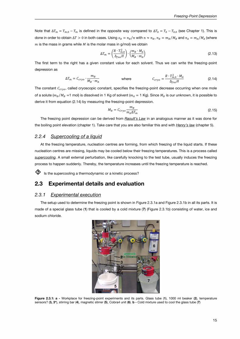
The setup used to determine the freezing point is shown in Figure 2.3.1a and Figure 2.3.1b in all its parts. It is
made of a special glass tube (1) that is cooled by a cold mixture (7) (Figure 2.3.1b) consisting of water, ice and
sodium chloride.
Figure 2.3.1: a - Workplace for freezing-point experiments and its parts. Glass tube (1), 1000 ml beaker (2), temperature sensors? (3, 3*), stirring bar (4), magnetic stirrer (5), Cobra4 unit (6). b - Cold mixture used to cool the glass tube (7)

Freezing-Point Depression
16
Turn on the Cobra4 unit (6), the computer and open the “excel” software and the “measure” software (see
Appendix 2.5.1 for basic instructions on how to perform the experiment).
Prepare the cold mixture by mixing water, ice and sodium chloride in the 1000 mL beaker (2). The amounts of
the components of the cold mixture have to be chosen in order to obtain a temperature of 𝑇 < -10 C. Fill the
1000 mL beaker completely with ice. Add deionized water up to the 800 mL calibration mark. Since part of the
ice is melting, add more ice until it does not melt anymore. To prevent the water from overflowing, part of it needs
to be poured into the basin from time to time. Once the ice does not melt anymore, pour sodium chloride on the
surface of the ice-water mixture and start immediately to stir it with the glass rod in order to dissolve the salt.
Check the temperature using the temperature sensor (3*). If 𝑇 > -10 C, add more salt and repeat the dissolving-
stirring procedure as described above. The temperature of the cold mixture increases with time, therefore it has
to be checked after each measurement and needs to be adjusted by adding ice and salt.
Clean the glass tube with deionized water. Add the stirring bar (4) carefully. In order to avoid breaking of the
glass tube, take care that the stirring bar does not fall from the top to the bottom of the glass tube.
In the first measurement, the freezing point of pure water is determined. Fill 25 mL of deionized water into the
glass tube using the pipette and mount the glass tube in the beaker with the cold mixture as deep as possible.
Place the first temperature sensor (3) in the middle of the glass tube. Take care, that it touches neither the
stirring bar nor the glass tube. Turn on the magnetic stirrer (5). Place the second temperature sensor (3*) into
the cold mixture in the beaker. This is used to monitor the temperature of the cold mixture in order to ensure that
it stays below -10 C.
Start the measurement. The measurement can be stopped if the temperature stayed constant for one minute.
Take the glass tube out of the cold mixture and liquefy the frozen sample by warming it with tap water from outside
(or using your hands). The same sample can be used for the next measurements. The freezing point of pure water
has to be determined three times. Calculate the average of the results for further data analysis. The following
measurements on the solutions have to be performed only twice. For further data analysis, always take
the average of the two individual results.
For the determination of the cryoscopic constant of water, prepare two solutions of urea in deionized water
(solutions A and B) for the next measurements:
Solution A: 2.5 g of urea in 25 mL of solution in deionized water
Solution B: 1.5 g of urea in 25 mL of solution in deionized water
The following measurements are performed in order to identify an unknown substance by determining its freezing
point. The unknown substance is available on the bench. Prepare the two following solutions (solutions C and
D):
Solution C: 1 g of unknown substance in 25 mL of solution in deionized water
Solution D: 2 g of unknown substance in 25 mL of solution in deionized water
In the last measurements, the degree of dissociation of sodium sulfate is determined. For this, prepare the
following solution (solution E):
Solution E: 0.75 g of sodium sulfate in 25 mL of solution in deionized water

Freezing-Point Depression
17
2.3.2 Data evaluation
Determine the freezing point of pure water.
Plot temperature vs. time for the two solutions of different urea concentration and use this to determine
the cryoscopic constant of water.
Determine the molecular weight of the unknown substance according to equation (2.15).
Determine the degree of dissociation of sodium sulfate using the experimentally determined cryoscopic
constant of water.
Perform an error analysis for all calculations.
2.4 Applications of the experiment and its theory
In organic and inorganic chemistry, the effect of freezing point depression can be applied to determine
the molecular weight of newly synthesized molecules. This method is called cryoscopy. Cryoscopy is
used in also food science [2.7 - 2.9].
Application of road salt to prevent ice formation on pavements and streets in winter.
Anti-freezing agent in the cars radiator to avoid freezing of the liquid cooling system.
Anti-freezing agents (e.g. glucose, glycerol, urea) produced naturally in the body of some insects and
frogs [2.10].
Analysis of freezing point depression is important in polymer science. [2.11]
2.5 Appendixes
2.5.1 Basic Instructions to use the software
Turn on the computer.
Login to your account using your lrz-username.
Open the Phywe “measure” software that you can find at the path
C:\Program Files (x86)\PHYWE\measure\measure.exe.
Click on “Experiment” followed by “Load configuration” to open the load configuration window (Figure
2.5.1) You find the configurations under “C:\Benutzer\Öffentlich”. Select the configuration needed for the
experiment you are working on.
Figure 2.5.1: Loading the configuration in the Phywe “measure” software.

Freezing-Point Depression
18
Open a new excel sheet and save it with a new data name.
Start the measurement by clicking on the red button in the left upper corner (Figure 2.5.2).
Figure 2.5.2: Starting the data collection in the Phywe “measure” software.
If the temperature is constant for one minute, stop the measurement by clicking on the black square in
the upper left corner (Figure 2.5.2).
Confirm the appearing window “send all data to measure” (Figure 2.5.3).
Figure 2.5.3: Data processing in order to save the data in the measure software.
Transfer the data to excel by clicking on “Measurement” “Export data” (Figure 2.5.4).
Figure 2.5.4: Export data to excel.
Select “Copy to clipboard” in the appearing window (Figure 2.5.5).
Figure 2.5.5: Copy data to clipboard.
Switch to excel and paste the data to your excel sheet.

Freezing-Point Depression
19
2.6 Literature
2.1 - P.W. Atkins, Physical Chemistry, 6th ed., Oxford University Press, Oxford (1998), pp. 163-182.
2.2 - P.W. Atkins and J. de Paula, Atkins’ Physical Chemistry, 8th ed., Oxford University Press, Oxford (2006),
pp. 136-156.
2.3 - R.E. Dickerson, H.B. Gray, M.Y. Darensbourg and D.J. Darensbourg, Prinzipien der Chemie, 2nd ed. (1988).
2.4 - G. Wedler, Lehrbuch der Physikalischen Chemie, 6th ed., Willey/VCH (2012).
2.5 - W.J. Moore, Grundlagen der Physikalischen Chemie, 1st ed., de Gruyter (1990).
2.6 - R. Brdicka, Grundlagen der Physikalischen Chemie, 15th ed., Wiley/VCH (1981).
2.7 - C.S. Chen, Effective Molecular Weight of Aqueous Solutions and Liquid Foods from the Freezing Point
Depression, Journal of Food Science, 51 (1986) 1537-1539.
2.8 - C.S. Chen, Thermodynamic Analysis of the Freezing and Thawing of Foods: Enthalpy and Apparent Specific
Heat, Journal of Food Science, 50 (1985) 1158-1162.
2.9 - J.B. Lahne and S.J. Schmidt, Gelatin-Filtered Consommé: A Practical Demonstration of the Freezing and
Thawing Processes, Journal of Food Science, 9 (2010) 53-58.
2.10 - K.B. Storey and J.M. Storey, Natural Freezing Survival in Animals, Ann. Rev. of Ecology and Systematics,
27 (1996) 365-386.
2.11 - B.B. Boonstra, F.A. Heckman and G.L. Taylor, Anomalous freezing point depression of swollen gels,
Journal of Applied Polymer Science, 12 (1986) 223-247.
20
3 Joule-Thomson Effect
3.1 Context and aim of the experiment
The aim of this experiment is to measure and interpret the Joule-Thomson coefficient of various gases. The
students are supposed to understand how the Joule-Thomson coefficient relates to the intermolecular forces in
general and to the van der Waals parameters 𝑎, 𝑏 and the second viral coefficient 𝐵, in particular. A quantitative
comparison of these parameters with the experimental results will be performed. Finally the influence of
temperature on the Joule-Thompson effect will be illustrated graphically and discussed within the concept of
inversion temperature [3.1 - 3.6].
3.1.1 Important concepts to know
Ideal and real gas: Lennard-Jones potential, van der Waals forces, dispersive London forces, van der Waals’
equation of state, Clausius’ virial expansion
Joule-Thomson-Coefficient: first law of thermodynamics, enthalpy, isenthalpic processes, inversion curve of the
Joule-Thomson-Coefficient
3.1.2 Most common questions to be answered
What is the difference between a reversible adiabatic, a reversible isothermal and an isenthalpic (Joule-
Thomson) expansion? Show these differences in a 𝑝 − 𝑉-diagram and explain what is happening along the
Lennard-Jones-potential. How do the internal energy 𝑈, the enthalpy 𝐻, the entropy 𝑆 and the temperature
𝑇 change during the processes?
Why does a real gas usually cool down during an isenthalpic expansion? What happens to an ideal gas? In
which situation does a real gas warm up instead cooling down?
Which qualitative relation exists between the Joule-Thomson effect (depending on the variable 𝑝) and the
Lennard-Jones potential (depending on the variable 𝑟)?
Which criteria need to be considered when looking for a gas with maximum Joule-Thomson effect? Which
of the gases investigated in this experiment would you start with and why?
3.1.3 Further preparations before the experiment
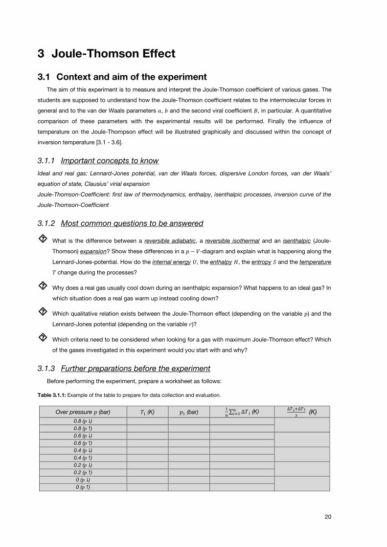
Before performing the experiment, prepare a worksheet as follows:
Table 3.1.1: Example of the table to prepare for data collection and evaluation.
Over pressure 𝑝 (bar) 𝑇1 (K) 𝑝1 (bar) 1
𝑛∑ ∆𝑇 𝑖𝑛𝑖=1 (K)
∆𝑇↓+∆𝑇↑
2 (K)
0.8 (𝑝 ↓)
0.8 (𝑝 ↑) 0.6 (𝑝 ↓)
0.6 (𝑝 ↑) 0.4 (𝑝 ↓)
0.4 (𝑝 ↑) 0.2 (𝑝 ↓)
0.2 (𝑝 ↑) 0 (𝑝 ↓)
0 (𝑝 ↑)

Joule-Thomson Effect
21
𝑇1 and 𝑝1 stand for the ambient temperature and the ambient pressure, respectively. 𝑝 ↓ and 𝑝 ↑ indicate the
series of measurement going from high to low pressure and from low to high pressure, respectively. ∆𝑇↓+∆𝑇↑
2
denotes the average of the temperature differences determined in the two series of measurement.
3.2 Theory
An adiabatic, irreversible expansion (=isenthalpic see below) of a real gas across a throttle (nozzle) in general
leads to a reduction of temperature. Such an effect is not expected in ideal gases; since it results from the
presence intermolecular interactions.
3.2.1 Internal energy and intermolecular interactions
The internal energy 𝑈 consists of the kinetic energy (energy of the translational, rotational and vibrational
degrees of freedom) of the molecules and of their potential energy, which, in our case, results from intermolecular
interactions. The contributions to 𝑈 can be specified by the following differential
𝑑𝑈 = (𝜕𝑈
𝜕𝑇)𝑉𝑑𝑇 + (
𝜕𝑈
𝜕𝑉)𝑇𝑑𝑉 (3.1)
The first term in equation (3.1) corresponds to the kinetic energy, while the second term arises due to the presence
of intermolecular interactions. Furthermore
(𝜕𝑈
𝜕𝑇)𝑉= 𝐶𝑉 (3.2)
where 𝐶𝑉 denotes the heat capacity at constant volume and depends on the number of thermodynamically active
degrees of freedom. Each degree of freedom retains the energy
𝑅 ∙ 𝑇/2 and thus contributes with 𝑅/2 to the heat capacity. Furthermore
(𝜕𝑈
𝜕𝑉)𝑇= 𝑝𝑐𝑜ℎ𝑒𝑠𝑖𝑜𝑛 (3.3)
where 𝑝𝑐𝑜ℎ𝑒𝑠𝑖𝑜𝑛 is the cohesion pressure. Since the differential is performed at constant temperature, i. e., at
constant kinetic energy, this term is a measure of the intermolecular interations: any change of volume results in
a change of the average distance ⟨𝑟⟩ and, accordingly, of the interaction between the molecules.
Let us now consider the special case of an adiabatic expansion (meaning that there is no heat exchange) into
vacuum (meaning that there is no work transferred to the surroundings). According to the first law of
thermodynamics, the internal energy 𝑈 must remain constant, i. e., 𝑑𝑈 = 0. At ordinary values of pressure and
temperature, the attractive interactions dominate and, consequently, an increase in average distance ⟨𝑟⟩ of the
molecules increases the interaction energy (compare Lennard-Jones potential, Figure 3.2.1).
Figure 3.2.1: The Lennard-Jones-potential is the intermolecular interaction (potential energy) between two uncharged particles plotted as a function of the distance 𝑟 for noble gases. It has a minimum at 𝑟𝑚𝑖𝑛 = 21/6 ∙ 𝑟𝐿𝐽 where 𝑟𝐿𝐽 is the Lennard-Jones radius
at which 𝐸𝐿𝐽 = 0. The depth of the well is the intermolecular binding energy 휀𝐿𝐽. The Lennard-Jones-radius increases with
increasing atomic mass, while simultaneously the binding energy becomes stronger and stronger. Note that for theoretical calculations of Joule-Thomson-coefficients the 1/r12 term is usually replaced by an exponential term (exp-6 potential) [3.1].

Joule-Thomson Effect
22
At intermolecular distances 𝑟 < 𝑟𝐿𝐽 repulsion occurs between molecules (Pauli principle), if 𝑟 > 𝑟𝐿𝐽 attraction
prevails (due to London dispersion force: instantaneous dipole–induced dipole forces). Since for an expansion
into vacuum the intermolecular distance 𝑟 increases to infinity (𝑟 → ∞), the interaction energy, i. e., the interaction
term (𝜕𝑈
𝜕𝑉)𝑇𝑑𝑉, increases. If the constrains of the experiment have been chosen to prohibit flow of energy from
the surroundings (𝑑𝑈 = 0), the kinetic term (𝜕𝑈
𝜕𝑇)𝑉𝑑𝑇 must decrease. Consequently, the amount of interaction
energy necessary for expansion can only be extracted from the internal kinetic degrees of freedom, which explains
the decreasing temperature. The less degrees of freedom are available, i. e., the smaller the heat capacity is, the
stronger this temperature decrease will be.
3.2.2 The Joule-Thomson-Experiment
Joule’s first attempt to verify intermolecular interactions failed, since the experiments were not conducted
under adiabatic conditions. To detect the temperature change he used a surrounding heat bath. However, due to
its high heat capacity, the heat bath provided all the energy necessary for expansion to the vacuum and thus the
proposed decrease in temperature was not detectable. In 1842, Joule und Thomson carried out the experiment
under improved constraints (Figure 3.2.2). i) The temperature change was not detected in a surrounding heat bath,
but directly in the adiabatically expanding gas (by thermally insulation of the gas from its surroundings); ii) the
experiment was conducted in a quasi-stationary mode, by leading a continuous stream of gas through a throttle
(or nozzle), generating a pressure drop from the initial pressure 𝑝𝑖𝑛𝑖𝑡𝑖𝑎𝑙 in front of the throttle to the final pressure
𝑝𝑓𝑖𝑛𝑎𝑙. (Note that in our experiment 𝑝𝑓𝑖𝑛𝑎𝑙 corresponds to the external pressure 𝑝1). The gas flowing out of the
throttle continuously provides freshly cooled gas over a longer period of time, thus making temperature changes
easily detectable.
Figure 3.2.2: Adiabatic Joule-Thomson experiment. A continuously flowing gas stream generates a pressure fall across a throttle leading to an expansion of the gas against the intermolecular forces. The stronger the attraction, the larger the detectable temperature decrease will be.
In the new experiment, the temperature changes were big enough to be detectable for even small pressure
differences. The Joule-Thomson coefficient is the temperature change per pressure unit
𝜇𝐽𝑇 = (𝜕𝑇
𝜕𝑝)𝐻
(3.4)
If multiplied with the heat capacity of the gas, 𝜇𝐽𝑇 is related to the change of the Lennard-Jones potential induced
by the change of the average distance ⟨𝑟⟩ of the molecules with pressure.
3.2.3 Thermodynamic analysis of the Joule-Thomson effect
Since the Joule-Thomson experiment (Figure 3.2.4) is performed under adiabatic conditions (meaning that
there is no heat flow from the system to the surroundings), we conclude from the first law of thermodynamics that
Δ𝑈 = 𝑤 (for the first law of thermodynamics see also paragraph 5.2.1). Then we calculate the work 𝑤 performed
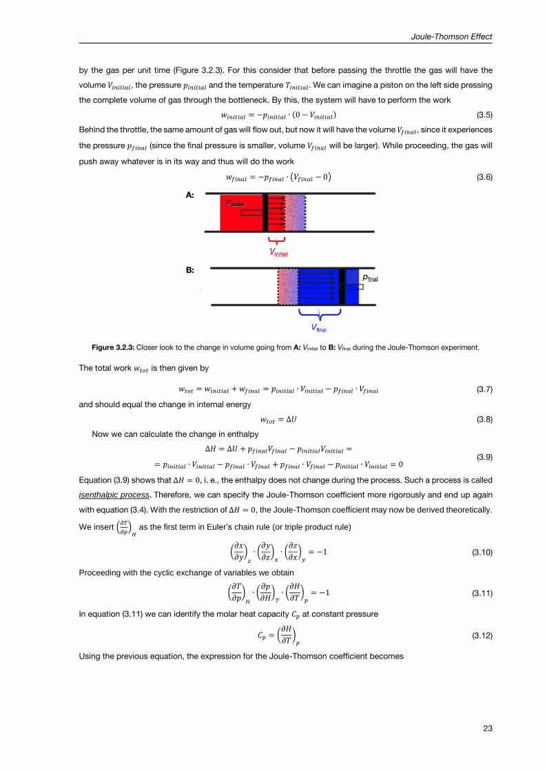
Joule-Thomson Effect
23
by the gas per unit time (Figure 3.2.3). For this consider that before passing the throttle the gas will have the
volume 𝑉𝑖𝑛𝑖𝑡𝑖𝑎𝑙, the pressure 𝑝𝑖𝑛𝑖𝑡𝑖𝑎𝑙 and the temperature 𝑇𝑖𝑛𝑖𝑡𝑖𝑎𝑙. We can imagine a piston on the left side pressing
the complete volume of gas through the bottleneck. By this, the system will have to perform the work
𝑤𝑖𝑛𝑖𝑡𝑖𝑎𝑙 = −𝑝𝑖𝑛𝑖𝑡𝑖𝑎𝑙 ∙ (0 − 𝑉𝑖𝑛𝑖𝑡𝑖𝑎𝑙) (3.5)
Behind the throttle, the same amount of gas will flow out, but now it will have the volume 𝑉𝑓𝑖𝑛𝑎𝑙, since it experiences
the pressure 𝑝𝑓𝑖𝑛𝑎𝑙 (since the final pressure is smaller, volume 𝑉𝑓𝑖𝑛𝑎𝑙 will be larger). While proceeding, the gas will
push away whatever is in its way and thus will do the work
𝑤𝑓𝑖𝑛𝑎𝑙 = −𝑝𝑓𝑖𝑛𝑎𝑙 ∙ (𝑉𝑓𝑖𝑛𝑎𝑙 − 0) (3.6)
Figure 3.2.3: Closer look to the change in volume going from A: Vinitial to B: Vfinal during the Joule-Thomson experiment.
The total work 𝑤𝑡𝑜𝑡 is then given by
𝑤𝑡𝑜𝑡 = 𝑤𝑖𝑛𝑖𝑡𝑖𝑎𝑙 + 𝑤𝑓𝑖𝑛𝑎𝑙 = 𝑝𝑖𝑛𝑖𝑡𝑖𝑎𝑙 ∙ 𝑉𝑖𝑛𝑖𝑡𝑖𝑎𝑙 − 𝑝𝑓𝑖𝑛𝑎𝑙 ∙ 𝑉𝑓𝑖𝑛𝑎𝑙 (3.7)
and should equal the change in internal energy
𝑤𝑡𝑜𝑡 = ∆𝑈 (3.8)
Now we can calculate the change in enthalpy
∆𝐻 = ∆𝑈 + 𝑝𝑓𝑖𝑛𝑎𝑙𝑉𝑓𝑖𝑛𝑎𝑙 − 𝑝𝑖𝑛𝑖𝑡𝑖𝑎𝑙𝑉𝑖𝑛𝑖𝑡𝑖𝑎𝑙 =
= 𝑝𝑖𝑛𝑖𝑡𝑖𝑎𝑙 ∙ 𝑉𝑖𝑛𝑖𝑡𝑖𝑎𝑙 − 𝑝𝑓𝑖𝑛𝑎𝑙 ∙ 𝑉𝑓𝑖𝑛𝑎𝑙 + 𝑝𝑓𝑖𝑛𝑎𝑙 ∙ 𝑉𝑓𝑖𝑛𝑎𝑙 − 𝑝𝑖𝑛𝑖𝑡𝑖𝑎𝑙 ∙ 𝑉𝑖𝑛𝑖𝑡𝑖𝑎𝑙 = 0 (3.9)
Equation (3.9) shows that ∆𝐻 = 0, i. e., the enthalpy does not change during the process. Such a process is called
isenthalpic process. Therefore, we can specify the Joule-Thomson coefficient more rigorously and end up again
with equation (3.4). With the restriction of ∆𝐻 = 0, the Joule-Thomson coefficient may now be derived theoretically.
We insert (𝜕𝑇
𝜕𝑝)𝐻
as the first term in Euler’s chain rule (or triple product rule)
(𝜕𝑥
𝜕𝑦)𝑧
∙ (𝜕𝑦
𝜕𝑧)𝑥∙ (𝜕𝑧
𝜕𝑥)𝑦= −1 (3.10)
Proceeding with the cyclic exchange of variables we obtain
(𝜕𝑇
𝜕𝑝)𝐻
∙ (𝜕𝑝
𝜕𝐻)𝑇∙ (𝜕𝐻
𝜕𝑇)𝑝= −1 (3.11)
In equation (3.11) we can identify the molar heat capacity 𝐶𝑝 at constant pressure
𝐶𝑝 = (𝜕𝐻
𝜕𝑇)𝑝 (3.12)
Using the previous equation, the expression for the Joule-Thomson coefficient becomes

Joule-Thomson Effect
24
𝜇𝐽𝑇 = (𝜕𝑇
𝜕𝑝)𝐻
= −1
(𝜕𝐻𝜕𝑇
)𝑝∙ (𝜕𝑝𝜕𝐻
)𝑇
= −
(𝜕𝐻𝜕𝑝
)𝑇
(𝜕𝐻𝜕𝑇
)𝑝
⇒ 𝜇𝐽𝑇 = −1
𝐶𝑝∙ (𝜕𝐻
𝜕𝑝)𝑇
(3.13)
For ideal gases, we know that the internal energy only depends on the temperature, not on the pressure or
the volume. In this case, the enthalpy is also a function of only the temperature, thus the term (𝜕𝐻
𝜕𝑝)𝑇= 0 results
in 𝜇𝐽𝑇 = 0. This is different for real gases. In the following, it is shown that in this case (𝜕𝐻
𝜕𝑝)𝑇≠ 0 and that this term
reflects intermolecular interactions. For the derivation of (𝜕𝐻
𝜕𝑝)𝑇 equations (3.14) and (3.15) need to be introduced.
The Gibbs’ fundamental equation of thermodynamics expresses the total differential of the enthalpy as
𝑑𝐻 = 𝑇 ∙ 𝑑𝑆 + 𝑉 ∙ 𝑑𝑝 (3.14)
and mathematically represents a summary of the first and the second law of thermodynamics.
The Maxwell equation
(𝜕𝑆
𝜕𝑝)𝑇
= −(𝜕𝑉
𝜕𝑇)𝑝 (3.15)
mathematically reflects the fact, that the Gibbs’ energy 𝐺 = 𝐻 − 𝑇𝑆 is a conserved quantity. Formally dividing
equation (3.14) by 𝑑𝑝 gives
(𝜕𝐻
𝜕𝑝)𝑇
= 𝑇 ∙ (𝜕𝑆
𝜕𝑝)𝑇
+ 𝑉 (3.16)
and further insertion of equation (3.15) provides
(𝜕𝐻
𝜕𝑝)𝑇
= −𝑇 ∙ (𝜕𝑉
𝜕𝑇)𝑝+ 𝑉 (3.17)
Finally, combination of equation (3.17) and equation (3.13) provides
𝜇𝐽𝑇 =1
𝐶𝑝∙ {𝑇 ∙ (
𝜕𝑉
𝜕𝑇)𝑝− 𝑉} (3.18)
For an ideal gas, the thermic expansion coefficient 𝛼 (in general ≡1
𝑉∙ (
𝜕𝑉
𝜕𝑇)𝑝) can be calculated easily by
𝛼𝑖𝑑𝑒𝑎𝑙 =1
𝑉∙ (𝜕𝑉
𝜕𝑇)𝑝=
𝑝
𝑛𝑅𝑇∙ (
𝜕 (𝑛𝑅𝑇𝑝
)
𝜕𝑇)
𝑝
=1
𝑇 (3.19)
Using this relation, equation (3.18) becomes
𝜇𝐽𝑇 =𝑉
𝐶𝑝∙ {𝛼𝑇 − 1} =
𝑉
𝐶𝑝∙ {
𝛼
𝛼𝑖𝑑𝑒𝑎𝑙− 1} (3.20)
The deviation of the thermal expansion in a real gas from the thermal expansion in an ideal gas results from
intermolecular interactions. Attractive forces lead to smaller expansion, while repulsive forces enhance thermal
expansion. Consequently, we find three different situations for the Joule-Thomson effect:
a) 𝛼 = 𝛼𝑖𝑑𝑒𝑎𝑙 ⟹ 𝜇𝐽𝑇𝑖𝑑𝑒𝑎𝑙 𝑔𝑎𝑠
= 0
b) 𝛼 > 𝛼𝑖𝑑𝑒𝑎𝑙 ⟹ 𝜇𝐽𝑇 > 0 ⟹ 𝑑𝑇 < 0, thus the gas cools down
c) 𝛼 < 𝛼𝑖𝑑𝑒𝑎𝑙 =1
𝑇⟹ 𝜇𝐽𝑇 < 0⟹ 𝑑𝑇 > 0, thus the gas warms up
Both 𝛼 and 𝛼𝑖𝑑𝑒𝑎𝑙 change with temperature, but differently. Thus the Joule-Thomson coefficient is a function
of temperature, and may even change sign at the so-called inversion temperature 𝑇𝑖𝑛𝑣𝑒𝑟𝑠, where 𝜇𝐽𝑇𝑇𝑖𝑛𝑣𝑒𝑟𝑠 = 0. This
is shown in Figure 3.2.4. Here, the temperature 𝑇 is plotted as a function of pressure 𝑝 at constant enthalpy 𝐻.
The corresponding theoretical derivation is given in paragraph 3.2.4 and appendix 3.5.4.

Joule-Thomson Effect
25
Figure 3.2.4: Isenthaplic processes in a 𝑝 − 𝑇 diagram at constant enthalpy. 𝜇𝐽𝑇 is the slope of the isenthalpic graph.
3.2.4 Derivation of the expansion coefficient and the Joule-Thomson coefficient
As already show before, we need the expansion coefficient 𝛼 of the real gas to calculate the Joule-Thomson
coefficient 𝜇𝐽𝑇
. We start with calculating 𝜕𝑉𝑚
𝜕𝑇. Since solving the van der Waals equation of state for the volume is
very cumbersome (cubic equation!), instead we solve the equation for the pressure and write the derivative with
time
𝑝 =𝑅𝑇
𝑉 − 𝑏−
𝑎
𝑉𝑚2 |∙
𝜕
𝜕𝑇 (3.21)
From this, we obtain a simpler equation with terms containing 𝜕𝑉𝑚
𝜕𝑇, which is easier to be solved
𝜕𝑝
𝜕𝑇= 0 =
𝜕
𝜕𝑇(
𝑅𝑇
𝑉𝑚 − 𝑏) −
𝜕
𝜕𝑇(𝑎
𝑉𝑚2) =
=𝑅(𝑉𝑚 − 𝑏) − 𝑅𝑇
(𝑉𝑚 − 𝑏)2∙𝜕𝑉𝑚𝜕𝑇
−−2𝑎
𝑉𝑚3 ∙
𝜕𝑉𝑚𝜕𝑇
(3.22)
we order the terms
𝑅
(𝑉𝑚 − 𝑏)= {
𝑅𝑇
(𝑉𝑚 − 𝑏)2−2𝑎
𝑉𝑚3} ∙
𝜕𝑉𝑚𝜕𝑇
(3.23)
and after introducing a common denominator for the term in {𝑅𝑇
(𝑉𝑚−𝑏)2 −
2𝑎
𝑉𝑚3}
𝑅𝑇𝑉𝑚
3 − 2𝑎(𝑉𝑚 − 𝑏)2
(𝑉𝑚 − 𝑏)2 ∙ 𝑉𝑚3 (3.24)
we can solve for 𝜕𝑉𝑚
𝜕𝑇
𝜕𝑉𝑚𝜕𝑇
=
𝑅(𝑉𝑚 − 𝑏)
𝑅𝑇𝑉𝑚3 − 2𝑎(𝑉𝑚 − 𝑏)2
(𝑉𝑚 − 𝑏)2 ∙ 𝑉𝑚3
=𝑅(𝑉𝑚 − 𝑏) ∙ 𝑉𝑚
3
𝑅𝑇𝑉𝑚3 − 2𝑎(𝑉𝑚 − 𝑏)2
(3.25)
Cancelling 𝑅 ∙ 𝑉𝑚3 leads to
𝜕𝑉𝑚𝜕𝑇
=(𝑉𝑚 − 𝑏)
𝑇 −2𝑎𝑅𝑉𝑚
∙ (𝑉𝑚 − 𝑏𝑉𝑚
)2
(3.26)
Finally, we obtain the expansion coefficient
𝛼 =
1
𝑉𝑚∙𝜕𝑉𝑚𝜕𝑇
=(𝑉𝑚 − 𝑏)
𝑉𝑚 ∙ 𝑇 −2𝑎𝑅∙ (𝑉𝑚 − 𝑏𝑉𝑚
)2
(3.27)
or, by introduction into equation (3.20), the Joule-Thomson coefficient

Joule-Thomson Effect
26
𝜇𝐽𝑇 =𝑉𝑚𝐶𝑝
(
(𝑉𝑚 − 𝑏)
𝑉𝑚 −2𝑎𝑅𝑇
∙ (𝑉𝑚 − 𝑏𝑉𝑚
)2 − 1
)
(3.28)
For further insights, see appendix 3.5.4.
3.2.5 Calculation of the inversion curve using the van-der-Waals equation of state
The inversion curve can directly be calculated from the van-der-Waals equation without any further
approximation. We get the sign change at 𝜇𝐽𝑇 = 0 at the inversion temperature. Accordingly to equation (3.20),
𝛼 = 1/𝑇 at these conditions and we get
𝛼 =
(𝑉𝑚 − 𝑏)
𝑉𝑚 ∙ 𝑇 −2𝑎𝑅∙ (𝑉𝑚 − 𝑏𝑉𝑚
)2 =
1
𝑇
(3.29)
Now, the terms of 𝑇 and 𝑉 have to be ordered and the expression is inserted in the van-der-Waals equation
(see appendix 3.5.5). This reveals the following expression for the inversion curve
𝑝𝑖𝑛𝑣 = √8𝑎𝑅𝑇𝑖𝑛𝑣𝑒𝑟𝑠
𝑏3−3
2∙𝑅𝑇𝑖𝑛𝑣𝑒𝑟𝑠
𝑏−
𝑎
𝑏2 (3.30)
Important: here, we have the inversion curve given as pressure as a function of temperature (Figure 3.2.5).
One could in principle solve for 𝑇, which would make things much more complicated. It is much easier to calculate
𝑝(𝑇) and plot it as a 𝑝 − 𝑇-diagram. After that, one may change the axes by mirroring with respect to the diagonal.
For a sketch, one may simply combine a rising √𝑇-graph (horizontal parabola) and a linearly falling 𝑇-graph
(straight line with negative slope). Of course, the inversion curve is only valid for positive values of 𝑝.
Figure 3.2.5: Inversion curve in reduced coordinates in a p-T-diagram.
3.3 Experimental details and evaluation
Your supervisor will provide the connection to two unknown gases, which should be identified by experimental
determination of their Joule-Thomson coefficients 𝜇. This can be determined experimentally by measuring the
temperature 𝑇𝑐𝑜𝑚𝑝 of the gas in its compressed state at 𝑝 = 𝑝𝑐𝑜𝑚𝑝 and the temperature 𝑇𝑒𝑥𝑝 in its expanded state
at 𝑝 = 𝑝1, where 𝑝1 is the ambient pressure. Plotting ∆𝑝 = 𝑝0 − 𝑝1 vs. ∆𝑇 = 𝑇𝑐𝑜𝑚𝑝 − 𝑇𝑒𝑥𝑝 should provide a straight
line with a slope 𝑚 = 𝜇. (Note that 𝑇𝑐𝑜𝑚𝑝 equals the ambient temperature and it is named 𝑇1 in the software used
in this experiment).
For each gas two series of measurement are performed. The first series of measurement starts at an
overpressure of 0.8 bar and goes down to ambient pressure, using pressure steps of ∆𝑝 = -0.2 bar. The second
series is performed in the opposite direction, starting from ambient pressure and going up to an overpressure of

Joule-Thomson Effect
27
0.8 bar, using pressure steps of ∆𝑝 = 0.2 bar. Thus, altogether there are four series of measurement to perform,
each consisting of five individual measurements. The data are used to determine the Joule-Thomson coefficient
graphically, according to equation (3.4).
Further, the Joule-Thomson coefficient should be determined theoretically using equation (3.28) from the
theory. The required van-der-Waals parameters are given in appendix 3.5.3.
3.3.1 Experimental execution
The setup used to measure the Joule-Thomson coefficient is shown in Figure 3.3.1 and Figure 3.3.2 in all its
parts. The glass tube (1) is equipped with a restrictor (2) and is wrapped in transparent plastic for safety reasons.
At one end of the glass tube there is an opening (3) where the gas under investigation flows in and at the other
end there is an opening (4) where the gas flows out. The high-pressure part (5) of the glass tube is developed to
stand overpressures up to 1,0 bar. A copper capillary (6) is used to equilibrate the flowing gas at ambient
temperature. Two temperature sensors (7) are used to measure the temperature of the gas flowing through the
glass tube. The temperature sensors are positioned nearby the restrictor, one in front of it and the other one
behind it, respectively. This allows measuring the temperature of the gas before (𝑇 = 𝑇𝑐𝑜𝑚𝑝) and after (𝑇 = 𝑇𝑒𝑥𝑝) it
flows through the restrictor. After passing the second sensor the temperature of the flowing gas will adapt to the
temperature of the surroundings. The pressure sensor (8) is positioned next to the opening where the gas flows
in. A needle valve (9) is used to regulate the pressure (9).
Figure 3.3.1: - Setup in all its parts used to determine the Joule-Thomson coefficient. (1) glass tube, (2) restrictor, (3) opening for gas influx, (4) opening for gas efflux, (5) high pressure part, (6) copper capillary, (7) temperature sensors and (8) pressure sensor.
Figure 3.3.2: - Setup in all its parts used to determine the Joule-Thomson coefficient. (8) pressure sensor, (9) needle valve, (10) Cobra3 unit, (11) main valve and (12) regulator.
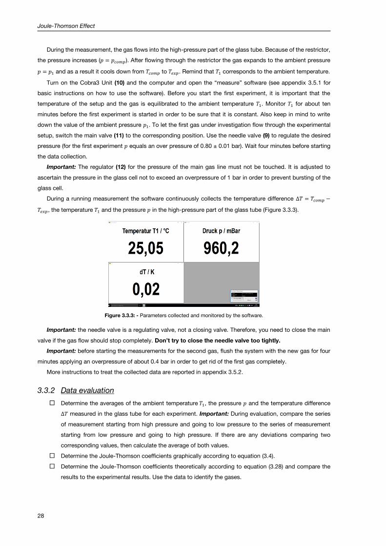
Joule-Thomson Effect
28
During the measurement, the gas flows into the high-pressure part of the glass tube. Because of the restrictor,
the pressure increases (𝑝 = 𝑝𝑐𝑜𝑚𝑝). After flowing through the restrictor the gas expands to the ambient pressure
𝑝 = 𝑝1 and as a result it cools down from 𝑇𝑐𝑜𝑚𝑝 to 𝑇𝑒𝑥𝑝. Remind that 𝑇1 corresponds to the ambient temperature.
Turn on the Cobra3 Unit (10) and the computer and open the “measure” software (see appendix 3.5.1 for
basic instructions on how to use the software). Before you start the first experiment, it is important that the
temperature of the setup and the gas is equilibrated to the ambient temperature 𝑇1. Monitor 𝑇1 for about ten
minutes before the first experiment is started in order to be sure that it is constant. Also keep in mind to write
down the value of the ambient pressure 𝑝1. To let the first gas under investigation flow through the experimental
setup, switch the main valve (11) to the corresponding position. Use the needle valve (9) to regulate the desired
pressure (for the first experiment 𝑝 equals an over pressure of 0.80 ± 0.01 bar). Wait four minutes before starting
the data collection.
Important: The regulator (12) for the pressure of the main gas line must not be touched. It is adjusted to
ascertain the pressure in the glass cell not to exceed an overpressure of 1 bar in order to prevent bursting of the
glass cell.
During a running measurement the software continuously collects the temperature difference ∆𝑇 = 𝑇𝑐𝑜𝑚𝑝 −
𝑇𝑒𝑥𝑝, the temperature 𝑇1 and the pressure 𝑝 in the high-pressure part of the glass tube (Figure 3.3.3).
Figure 3.3.3: - Parameters collected and monitored by the software.
Important: the needle valve is a regulating valve, not a closing valve. Therefore, you need to close the main
valve if the gas flow should stop completely. Don’t try to close the needle valve too tightly.
Important: before starting the measurements for the second gas, flush the system with the new gas for four
minutes applying an overpressure of about 0.4 bar in order to get rid of the first gas completely.
More instructions to treat the collected data are reported in appendix 3.5.2.
3.3.2 Data evaluation
Determine the averages of the ambient temperature 𝑇1, the pressure 𝑝 and the temperature difference
∆𝑇 measured in the glass tube for each experiment. Important: During evaluation, compare the series
of measurement starting from high pressure and going to low pressure to the series of measurement
starting from low pressure and going to high pressure. If there are any deviations comparing two
corresponding values, then calculate the average of both values.
Determine the Joule-Thomson coefficients graphically according to equation (3.4).
Determine the Joule-Thomson coefficients theoretically according to equation (3.28) and compare the
results to the experimental results. Use the data to identify the gases.

Joule-Thomson Effect
29
Calculate (equation (3.30)) and draw the complete inversion curve of CO2 using the corresponding van-
der-Waals coefficients and the heat capacity 𝐶𝑝 provided in Table 3.5.1.
Perform an error analysis for all calculations.
3.4 Applications of the experiment and its theory
Hampson-Linde cycle (liquefaction of air).
Due to the decrease in pressure by transferring gas from soil to pipelines, the gas cools down and the
surrounding area of the pipelines run the risk of freezing [3.5].
Leakage of high-pressure gas from a pipeline [3.6].
Risk of freezing of diving regulators.
Separation of gaseous mixtures by gas permeation, e.g., enrichment of oxygen from air and separation
of methane from biogas [3.7].
Generation of molecular beams for spectroscopy (Knudsen beam, supersonic beam).
Mode of operation of refrigerators and heat pumps.
3.5 Appendixes
3.5.1 Basic instructions to use the software
Turn on the Cobra3 Unit.
Turn on the computer.
Login to your account using your lrz-username.
Open the Phywe “measure” software that you can find at the path
C:\Program Files (x86)\PHYWE\measure\measure.exe.
Start the measurement by clicking on the red button in the left upper corner (Figure 3.5.1).
Figure 3.5.1: Starting the interface in the Phywe “measure” software.
Click on “Weiter” in the appearing window (Figure 3.5.2).

Joule-Thomson Effect
30
Figure 3.5.2: Starting the interface in the Phywe “measure” software.
Write down the value of the ambient pressure.
Switch the main valve to the position of the first gas under investigation.
Use the needle valve to regulate the gas pressure to an over pressure of 0.80 ± 0.01 bar.
Wait four minutes before you start the experiment.
Start the experiment by clicking on “Messung starten” (Figure 3.5.3)
Figure 3.5.3: Starting an experiment.
The measurement takes 20 seconds and stops automatically.
3.5.2 Instruction for data treatment
After finishing one series of measurement the data is treated before the next series of measurement is
started.
Use the computer software to calculate the averages of the ambient temperature, the pressure and the
temperature difference ∆𝑇 measured in the glass tube. This is done individually for each single
measurement within the series. To choose a single experiment click on the corresponding measuring
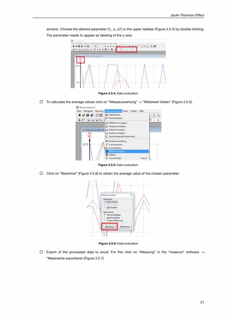
Joule-Thomson Effect
31
window. Choose the desired parameter (𝑇1, 𝑝, ∆𝑇) in the upper taskbar (Figure 3.5.4) by double clicking.
The parameter needs to appear as labeling of the y-axis.
Figure 3.5.4: Data evaluation.
To calculate the average values click on “Messauswertung” “Mittelwert bilden” (Figure 3.5.5).
Figure 3.5.5: Data evaluation.
Click on “Berechne” (Figure 3.5.6) to obtain the average value of the chosen parameter.
Figure 3.5.6: Data evaluation
Export of the processed data to excel: For this click on “Messung” in the “measure” software
“Messwerte exportieren (Figure 3.5.7).

Joule-Thomson Effect
32
Figure 3.5.7: Data export.
“In Zwischenablage kopieren” (Figure 3.5.8). Then change to the excel software and paste the values.
Figure 3.5.8: Data export.
Go back to the “measure” software and close the measuring window corresponding to the data you have
just analyzed.
Repeat the procedure for all measurement within the measuring series.
3.5.3 Van-der-Waals parameters
Table 3.5.1: Van-der-Waals coefficients a and b and heat capacity Cp for different gases.
a (l2bar/mol2) b (l/mol) Cp (J/(Kmol))
CO2 3.592 0.04267 37.14
He 0.03457 0.0237 20.79
N2 1.39 0.03913 29.14
3.5.4 Further implementations in the derivation of the Joule-Thomson coefficient for
real gases
𝛼
𝛼𝑖𝑑𝑒𝑎𝑙=
(𝑉𝑚 − 𝑏)
𝑉𝑚 −2𝑎𝑅𝑇
∙ (𝑉𝑚 − 𝑏𝑉𝑚
)2 =
(𝑉𝑚 − 𝑏)
(𝑉𝑚 − 𝑏) + 𝑏 −2𝑎𝑅𝑇
∙ (𝑉𝑚 − 𝑏𝑉𝑚
)2 ⇒
𝛼
𝛼𝑖𝑑𝑒𝑎𝑙< 1
if 𝑏 >2𝑎
𝑅𝑇∙ (
𝑉𝑚−𝑏
𝑉𝑚)2
(3.31)
Insertion into van-der-Waals equation:

Joule-Thomson Effect
33
𝑏 ∙ (𝑉𝑚
𝑉𝑚 − 𝑏)2
= 𝑏 ∙ (1 +𝑏
𝑉𝑚 − 𝑏)2
= 𝑏 ∙ (1 + 𝑏 ∙𝑝 +
𝑎𝑛2
𝑉2
𝑛𝑅𝑇)
2
>2𝑎
𝑅𝑇 (3.32)
This can be summarized as follows
Again, we have difficulties with inserting 𝑉𝑚 from the van-der-Waals equation. In order to avoid higher powers
of 𝑉𝑚, we can exploit a virial expansion instead, and drop higher powers of 𝑉𝑚. Thus we could reconstruct the
isenthalpic curves in a 𝑇 − 𝑝 diagramm.
∗= 1 −2𝑎
𝑅𝑇∙ (
𝑉𝑚
𝑉𝑚−𝑏)2 is the only term, that may change its sign. Further, we can see
a) (𝑉𝑚−𝑏
𝑉𝑚) is always smaller than 1. The larger 𝑏 (repulsion), the smaller the term * will be, which is
subtracted from 1, the more positive is 𝜇𝐽𝑇 . repulsion dominates and leads to heating!
b) The larger a is compared to 𝑅𝑇, the larger the term * will be, the more negative is 𝜇𝐽𝑇 . attraction
dominates and leads to cooling!
The exact position of sign change of 𝜇𝐽𝑇 can be delineated with inversion line.
3.5.5 Further implementations in the derivation of the inversion temperature for real
gases
Ordering the terms of equation (3.29) and insertion into the van-der-Waals equation
(3.33)
(3.34)
(3.35)

Joule-Thomson Effect
34
3.5.6 Virial coefficient
The Joule-Thomson coefficient is closely related to the second viral coefficient (B in equation (3.36) and BV in
equation (3.37):
𝑍 = 1 + 𝐵 ∙ 𝑝 + 𝐶 ∙ 𝑝2 +⋯ (3.36)
𝑍 = 1 +𝐵𝑉𝑉+𝐶𝑉𝑉2 +⋯ (3.37)
Digression: The second virial coefficient is an extremely useful quantity, since it is directly related to the
Lennard-Jones pair interaction potential 𝐸𝐽𝑇(𝑟). Since in a gas the distances between particles are statistically
distributed, one has to integrate any pair interaction potential 𝑈(𝑟) over all possible distances between the
particles. This relation is quantified in cluster integrals that are derived in statistical mechanics. It turns out, that
(because of the integration) it is difficult to exactly derive the exact form of 𝑈(𝑟) = 𝐸𝐽𝑇(𝑟).
3.6 Literature
3.1 - P.W. Atkins, Physical Chemistry, 6th ed., Oxford University Press, Oxford (1998), pp. 45-90.
3.2 - P.W. Atkins and J. de Paula, Atkins’ Physical Chemistry, 8th ed., Oxford University Press, Oxford (2006),
pp. 28-67.
3.3 - G. Wedler, Lehrbuch der Physikalischen Chemie, 6th ed., Willey/VCH (2012).
3.4 - R. Brdicka, Grundlagen der Physikalischen Chemie, 15th ed., Wiley/VCH (1981).
3.5 - K.C. Cheng and J.-W. Ou, Joule-Thomson Effects on Turbulent Graetz Problems for Gas Flow in Pipes with
uniform wall temperature, The Canadian Jounal of Chemical Engineering, 56 (1978) 31-36.
3.6 - R. Tu, Q. Xie, J. Yi, K. Li, X. Zhou and X. Jiang, An Experimental Study on the Leakage Process of High
Pressure CO2 from a Pipeline Transport System, Greenhouse Gases: Science and Technology, 4 (2014) 777-
784.
3.7 - R. Rautenbach and W. Dahm, Oxygen and Methane enrichment – a Comparison of Module Arrangements
in Gas Permeation, Chemical Engineering & Technology, 10 (1987) 256-261.

35
4 Combustion Enthalpy via Bomb Calorimetry
4.1 Context and aim of the experiment
In this experiment, the internal energy provided by the combustion of an organic compound is measured using
the method of bomb calorimetry. From the measured internal energy of the reaction at constant volume, the
reaction enthalpy of the combustion of the compound can be determined [4.1 - 4.3].
4.1.1 Important concepts to know
First law of thermodynamics, work, heat, internal energy, state function, intensive and extensive properties,
reaction enthalpy, exothermic and endothermic reaction, exergonic and endergonic reaction, calorimetry,
combustion enthalpy, adiabatic system, heat capacity at constant volume, heat capacity at constant pressure.
4.1.2 Most common questions to be answered
Why is the heat capacity at constant pressure 𝐶𝑝 always larger than that at constant volume 𝐶𝑉?
Consider a certain amount of heat being released during combustion of a sample in a calorimeter. Will the
induced ∆𝑇 be higher, if the measurement is performed at constant volume or at constant pressure? Why?
What is the statement of the first law of thermodynamics?
What is the definition of enthalpy?
What are the definitions of exergonic, endergonic, exothermic and endothermic reactions?
What are the prerequisites for a combustion reaction to occur?
4.1.3 Further preparations before the experiment
Before performing the experiment, prepare a worksheet for all five measurements as follows:
Table 4.1.1: Example of the table to prepare for data collection and evaluation.
sample ∆𝑇
[K] ∆𝑇𝑎𝑣𝑒𝑟𝑎𝑔𝑒 [K]
−𝑚𝑐𝑎𝑙 ∙ Δ𝑟𝐻𝑐𝑎𝑙
𝑀𝑐𝑎𝑙 ∙ Δ𝑇𝑐𝑎𝑙,𝑎𝑣𝑒𝑟𝑎𝑔𝑒
[J/K]
𝐶𝑐𝑎𝑙 ∙ Δ𝑇𝑎𝑣𝑒𝑟𝑎𝑔𝑒
[J]
benzoic acid
𝑚𝑐𝑎𝑙=
sucrose
𝑚𝑠𝑢𝑐𝑟𝑜𝑠𝑒=
4.2 Theory
The energy conversion during a chemical reaction can partly be absorbed or released as heat energy and
partly be utilized or expended as work. Calorimetry is the most established method for the study of heat transfer
during chemical and physical reactions.

Combustion Enthalpy via Bomb Calorimetry
36
4.2.1 Heat transactions, internal energy and reaction enthalpy
In thermodynamics, the total energy of a system is called its internal energy 𝑈. The internal energy is the sum
of the kinetic and the potential energy of all molecules in the system. It is a so-called state function since it is path
independent. This means that its value depends only on the current state of the system and not on how the state
has been reached. The thermodynamic state itself is characterized by variables like pressure 𝑝, temperature 𝑇,
volume 𝑉 and amount of substance 𝑛. Changing one of these state variables results in a change in the internal
energy. The internal energy is further an extensive property, meaning that it is additive for subsystems. Take care
that you are familiar with the terms of intensive and extensive property. According to the first law of
thermodynamics, the change in internal energy 𝑑𝑈 of a system is generally given by the amount of energy 𝛿𝑞
absorbed or released by the system in form of heat and the work 𝛿𝑤 done on or by the system
𝑑𝑈 = 𝛿𝑞 + 𝛿𝑤 (4.1)
Work and heat are not state functions and therefore their prefix in equation (4.1) is “𝛿” instead of “𝑑” in order to
express infinitesimal changes. A measurable change in internal energy during the reaction of a system (internal
reaction energy) is thus given by
∆𝑟𝑈 = 𝑞 + 𝑤 (4.2)
In equation (4.1), the work can be further separated in expansion work 𝛿𝑤𝑒𝑥𝑝 and work in addition to the expansion
work 𝛿𝑤𝑒. The latter could be the electrical work of driving a current through a circuit.
𝑑𝑈 = 𝛿𝑞 + 𝛿𝑤𝑒𝑥𝑝 + 𝛿𝑤𝑒 (4.3)
If the system is kept at constant volume, it cannot do expansion work and thus 𝛿𝑤𝑒𝑥𝑝 = 0. If the system is further
incapable of doing any other kind of work, then 𝛿𝑤𝑒 = 0 too, and equation (4.3) becomes
𝑑𝑈𝑉 = 𝛿𝑞𝑉 (4.4)
The subscript in 𝑑𝑈𝑉 and 𝛿𝑞𝑉 implies a change at constant volume. If the system passes from state A to state B
and during this exchanges heat with the surroundings, the measurable change in internal reaction energy is given
by
∆𝑟𝑈𝑉 = 𝑞𝑉 (4.5)
Equation (4.5) indicates that, when a change of state happens in a system at constant volume, by measuring the
energy supplied to it (𝑞𝑉 > 0, endothermic reaction) or obtained from it as heat (𝑞𝑉 < 0, exothermic reaction), we
are actually measuring the change in its internal energy. Comparison of equation (4.5) to the definition of enthalpy
d𝐻 = 𝑑𝑈 + 𝑝 ∙ 𝑑𝑉 (4.6)
and assuming that the volume of the system is constant (e. g., the involved components are either liquid or solid),
then Δ𝑟𝑉 and thus 𝑝 ∙ Δ𝑟𝑉 can be neglected and the reaction enthalpy equals the internal reaction energy
∆𝑟𝐻𝑉 = ∆𝑟𝑈𝑉 (4.7) Thus we can conclude that, measuring 𝑞𝑉 released or absorbed as heat during a reaction at constant volume
directly reveals the corresponding reaction enthalpy ∆𝑟𝐻𝑉.
4.2.2 Combustion reactions
Generally, the prerequisites for a combustion reaction to occur are i) the presence of an adequate amount of
an inflammable compound that has to be ii) in contact with an oxidant (generally oxygen) and iii) a high enough
ignition temperature in the surrounding of the inflammable compound. The latter point is necessary to overcome
the activation energy of the combustion reaction, and thus to start the reaction (ignition). As soon as part of the
compound has burned, the thereby released heat provides the activation energy for further combustion. For the
definition and meaning of the activation energy, see chapter 8.

Combustion Enthalpy via Bomb Calorimetry
37
Combustion reactions are usually exothermic, i. e., during the reaction energy is released as heat. For that
kind of reactions, the standard reaction enthalpy ∆𝑟𝐻0 < 0. Take care that you are familiar with the difference
between exothermic/endothermic and exergonic/endergonic reactions and with the meaning of the superscript
“0”. The enthalpy of combustion of a certain compound corresponds to its heating value (HV) also called calorific
value (CV). During combustion, water is produced either as liquid or vapour. If water is produced as liquid, the
amount of heat produced is maximum, since no heat is lost to vaporize the water, providing the so-called higher
heating value (HHV or higher calorific value HCV). If water is produced as vapour, the amount of heat produced is
lower, since some heat is lost as enthalpy of vaporization of water, providing the so-called lower heating value
(LHV or lower calorific value LCV).
4.2.3 Bomb calorimetry
Bomb calorimetry is the most established method to determine the combustion enthalpy at constant volume
of hydrocarbons. A schematic representation of a bomb calorimeter is shown in Figure 4.2.1.
Figure 4.2.1: Schematic representation of the design of a bomb calorimeter (adapted from [4.4]).
The calorimeter consists of a calorimetric bomb inside which the combustion reaction takes place. The
calorimetric bomb is designed to withstand heat and pressure and acts as a closed system. It is immersed in a
stirred Dewar (also called calorimeter vessel) filled with a known volume of water. The water in the Dewar prevents
heat flow from the calorimeter to its surroundings. Thus, the combustion reaction occurs under adiabatic
conditions. Further, there is an ignition unit used to start the combustion of the sample by application of a short
electric spark. This is necessary in order to overcome the activation energy of the combustion reaction (see
chapters 8). The calorimetric bomb is usually made of stainless steel and therefore the combustion reaction occurs
at constant volume. Often, a small amount of water is present in the calorimeter bomb in order to ensure that the
water vapour in the bomb is saturated. The advantage of this is, that the heat of vaporization of water does not
have to be taken into account in further data analysis.
During the measurement, a known amount of sample is ignited and is completely burned in the presence of
an oxygen excess, which is necessary to ensure fast and complete combustion. Since the combustion reaction
takes place at constant volume, equations (4.5) and (4.7) are valid. The heat of combustion released is absorbed
by the water in the calorimetric vessel and results in a measureable temperature increase ∆𝑇 = 𝑇𝑓𝑖𝑛𝑎𝑙 − 𝑇𝑖𝑛𝑖𝑡𝑖𝑎𝑙. In
order to convert ∆𝑇 to a reaction heat, the heat capacity of the calorimeter has to be known (for the definition and
meaning of the heat capacity and for the discrimination of the heat capacity at either constant volume or constant
pressure, see references [4.1, 4.2]). This can be determined by burning a fixed mass of a calibration sample (often
benzoic acid, see equation (4.8)) for which the combustion heat is exactly known.
2 𝐶6𝐻5𝐶𝑂𝑂𝐻(𝑠) + 15𝑂2(𝑔) → 14𝐶𝑂2(𝑔) + 6𝐻2𝑂(𝑙) (4.8)

Combustion Enthalpy via Bomb Calorimetry
38
Alternatively, the calibration can be done by measuring ∆𝑇 upon applying a known amount of heat by passing a
current from a source of known potential through a heater for a known period of time. Using the strategy of burning
a calibration sample, the heat capacity of the calorimeter 𝐶𝑐𝑎𝑙 can be determined via the equations
𝑄 = −𝑚𝑐𝑎𝑙 ∙ ∆𝑟𝐻𝑉,𝑐𝑎𝑙
𝑀𝑐𝑎𝑙 (4.9)
𝐶𝑐𝑎𝑙 =𝑄
∆𝑇𝑐𝑎𝑙 (4.10)
where ∆𝑟𝐻𝑉,𝑐𝑎𝑙 denotes the molar combustion enthalpy of the calibration sample (-3228 ± 4 kJ/mol for benzoic
acid [4.5]). 𝑚𝑐𝑎𝑙 is the amount of the used calibration substance and is given by the mass of the burned pellet
minus the mass of the igniter wire. 𝑀𝑐𝑎𝑙 is the molecular mass of the calibration substance. ∆𝑇𝑐𝑎𝑙 is the measured
temperature change during the combustion of the calibration substance.
Since the enthalpy is a state function, according to Hess’s law [4.1], any standard enthalpy of reaction ∆𝑟𝐻0
can be calculated from the standard enthalpy of formation ∆𝑓𝐻0 of each reactant and product, multiplied by their
stoichiometric coefficient in the reaction, according to the equation
∆𝑟𝐻0 = ∑ 𝜈𝑗 ∙ ∆𝑓𝐻𝑗
0
𝑃𝑟𝑜𝑑𝑢𝑐𝑡𝑠, 𝑗
− ∑ 𝜈𝑖 ∙ ∆𝑓𝐻𝑖0
𝑅𝑒𝑎𝑐𝑡𝑎𝑛𝑡𝑠, 𝑖
(4.11)
4.3 Experimental details and evaluation
In this experiment, the combustion of sucrose is investigated using bomb calorimetry. The corresponding
stoichiometric reaction is
𝐶12𝐻22𝑂11(𝑠) + 12𝑂2(𝑔) → 12𝐶𝑂2(𝑔) + 11𝐻2𝑂(𝑙) (4.12)
The recorded data are used to calculate the heat capacity of the calorimeter 𝐶𝑐𝑎𝑙, the internal reaction energy
∆𝑟𝑈𝑉 and from this the reaction enthalpy ∆𝑟𝐻𝑉 for reaction (4.12).
4.3.1 Experimental execution
The setup used to determine the heat transfer during combustion is shown from Figure 4.3.1 to Figure 4.3.4.
Figure 4.3.1: Calorimetric setup used for the determination of heat transfer during a chemical reaction; (1) calorimetric bomb, (2) calorimeter vessel, (3) temperature sensor, (4) black connector cords/firing leads, (5) power supply of the ignition unit, (6) magnetic stirrer and (7) outlet valve.

Combustion Enthalpy via Bomb Calorimetry
39
The calorimetric bomb (1) is immersed in the calorimeter vessel (2), also called dewar. Further, a temperature
sensor (3) is immersed in the calorimeter vessel. The temperature sensor is connected to the digital temperature
meter and measures the temperature of the water in the calorimeter vessel. The black connector cords (4) connect
the power supply (5) of the ignition unit to the calorimetric bomb (for details see Figure 4.3.2).
Figure 4.3.2: Individual parts of the calorimeter bomb: (8) pressure vessel, (9) O-ring-seal, (10) lid, (11) 4 mm connection socket, (12) control valve of the bomb, (13) quick-lock-coupling, (14) ceramic-disc, (15) nickel-electrode, (16) ferrule, (17) contacts for the nickel electrode, (18) quartz sample vessel and (19) sample vessel bracket.
The water in the calorimeter has to be stirred before, during and after the measurement using a magnetic
stirrer (6), in order to ensure homogeneous temperature. A detailed view of the calorimetric bomb and its coupling
parts are shown in Figure 4.3.2 and Figure 4.3.3, respectively. Figure 4.3.4 shows the details of the pressure
reducer of the oxygen pressure cylinder.
Figure 4.3.3: Coupling parts of the calorimeter bomb. (11) 4mm connection socket, (20) clamping ring, (21) quick connector and (22) control valve of the calorimetric bomb.
Figure 4.3.4: Pressure reducer on the oxygen cylinder. (7) outlet valve, (23) work manometer, (24) main valve of the oxygen bottle and the venting connection (25).

Combustion Enthalpy via Bomb Calorimetry
40
Fill the calorimeter vessel (2) with 850 ± 1 g of deionized water using the technical balance available in the lab.
Place the magnetic stirring bar in the calorimeter vessel carefully and switch on the magnetic stirrer (6).
The investigated substances, sucrose and benzoic acid, are available as powders. In order to ensure fast
combustion during the reaction the surface of the substances has to be large. To achieve this, only benzoic acid
have to be ground in a mortar. Weigh about 450 mg of substance in a weighing dish. After this, cut a piece of
about 10 cm length from the iron wire and weigh it too. The iron wire will be necessary for ignition of the substance.
Form the iron wire in such a manner that a small coil is formed in the middle to provide later a good grip on the
pellet.
Use the pellet-pressing die placing it in a vertical position and put the small steel rod in the cylinder to close
the bottom end of the borehole. Carefully insert the coil of the iron wire into the borehole, such that the ends of
the wire are positioned in the guiding grooves of the pellet press. Insert the large rod from above and press briefly
in order to press the coil of the iron wire plain. Fill the weighted substance into the hole using a funnel. Again insert
the large rod from above and compress the substance a little. Now fit the assembled pellet-pressing die in the
vice and carefully apply pressure on it, so that a solid pellet is formed from the substance. Take care, not to shear
off the ends of the ignition wire during preparation of the pellet. To get the pellet out of the press, hold the pellet
press over a plastic pan and turn it upside down. Grasp the long steel rod in the closed hole and help yourself
with a rubber mallet to get the pellet out. Weigh the pellet with an accuracy of 1 mg using the analytical balance.
It is essential to apply the right pressure during pellet preparation. If the pellet is too compact, then
combustion is hindered. On the other hand, the pellet will fall apart if the applied pressure is too small.
Now, the pellet can be introduced into the calorimetric bomb. To do this, put the pellet carefully in the quartz
sample vessel (18) using a spatula. Take care, that the coil of the iron wire is positioned near the vessel head,
because the pellet should be located above the centre of the sample vessel, so that it can burn there after the
ignition wire has burned out. This is important for proper combustion of the substance. The sample vessel can
now be fixed in the sample vessel bracket (19). Subsequently, fix the lid and the corresponding components (11-
13) to a stand using a clamp and fix the sample vessel bracket (19) by introducing the ends of the iron wire in the
contacts for the nickel-electrode (17) using tweezers. The overlaying parts of the iron wire need to be wrapped
around the nickel electrodes (15); then push the ferrules (16) downwards to fix the iron wire. Finally, the nickel-
electrode and the sample vessel bracket including the sample are introduced in the pressure vessel. Ensure that
the O-ring seal (9) is dust-free and the lid (10) is placed correctly. The calorimetric bomb is closed using the
clamping ring (20). Subsequently, the prepared calorimetric bomb is immersed as deep as possible in the water-
filled calorimetric vessel and is fixed to the stand using a clamp. Take care, that the quick connector (21) of the
calorimeter bomb and the clamping ring (20) are pointing in the same direction in order that there is enough space
for introduction of the temperature sensor (3). Fix the temperature sensor such that its tip is located about at the
same height as the sample in the bomb.
Before the calorimetric bomb is filled with oxygen, it is important to ensure that the outlet valve (7) is well
closed. Introduce the pressure hose in the quick connector (21) of the calorimetric bomb. Ensure that the venting
connection (25) is closed then open the main valve (24) of the oxygen bottle and check that the pressure at the
work manometer (23) is adjusted to 9 bar. Open the outlet valve (7) while keeping the control valve (22) of the
calorimetric bomb closed. As soon as the pressure stays constant, open carefully the control valve (22) of the
calorimetric bomb and by this oxygen flows in it. Once the calorimetric bomb is filled with oxygen, close its control
valve (22), the main valve (24) and the outlet valve (7) of the oxygen bottle, slowly and carefully open the venting
connection (25). Be sure that the power supply is turned off, introduce the black connector cords (4) of the
power supply (5) in the connection socket (11) of the lid and adjust the voltage of the power supply to 15 V. The

Combustion Enthalpy via Bomb Calorimetry
41
power supply needs to be employed manually in order to initiate the combustion; this is done just turning on the
main switch on the backside of the power supply.
The measurements are carried out using the Cobra 3 software. For basic instructions how to use the software
and how to handle the power supply in order to initiate the combustion, see appendix 4.5.1.
Important: After each single experiment, it is important to release excess oxygen and the gases that evolved
during the reaction before opening the calorimetric bomb. To do this, open the venting connection (25) and
then the control valve (22) of the calorimetric bomb slowly and carefully. The supervisor has to be present,
when the students execute this procedure for the first time. The calorimetric bomb may only be opened and
disassembled when all gases are purged out. To purge the pressure hose before the next measurement you
should slightly open the outlet valve (7) for a few seconds, after closing the venting connection (25).
The nickel-electrode needs to be cleaned after each experiment using a paper towel to get rid of
residues of the iron wire and carbon black.
The first measurements deal with the determination of the heat capacity 𝐶𝑐𝑎𝑙 of the calorimeter by analysing
the combustion of benzoic acid. The experiment on the combustion of benzoic acid has to be performed three
times and the average of the determined single ∆𝑇 values is used for calculation of 𝐶𝑐𝑎𝑙. In the subsequent
measurements, the release of heat during the combustion of sucrose is determined. This experiment has to be
performed three times as well and the average of the determined ∆𝑇 values is, together with 𝐶𝑐𝑎𝑙, used to
determine the enthalpy of the combustion of sucrose.
4.3.2 Data evaluation
Determine the heat capacity 𝐶𝑐𝑎𝑙 of the calorimeter applying equations (4.7) and (4.10) to the data
collected on the combustion reaction of benzoic acid. Check if the mass of the iron wire can be neglected
in these calculations.
Determine the molar combustion enthalpy of sucrose using the experimentally determined 𝐶𝑐𝑎𝑙 and
compare it with the literature value.
Calculate for all the combustion reaction considered their standard combustion enthalpy from the
standard enthalpies of formation of reactants and products available from [4.10].
Perform an error analysis for all calculations.
4.4 Applications of the experiment and its theory
Combustion enthalpies determined by calorimetric measurements are used to indirectly determine the
enthalpy of formation of inorganic and organic chemical compounds (Hess’s law). This is important for
thermodynamic investigation of flammable substances. Furthermore, combustion enthalpies are used
to calculate standard reaction energies and enthalpies of any chemical reaction [4.6].
Combustion reactions are very important reactions which provide energy, e.g. the combustion of
alkanes in power stations, heating installations and combustion engines. Their higher heating value is
the maximum energy that they could provide.
Determination of calorific values of fuel oils, motor fuels, flammable waste (waste combustion and
recycling industry), explosive agents, building materials (chalk and cement industry) etc. [4.7].
Determination of calorific values of foods, this is how the food calories are measured. [4.8].

Combustion Enthalpy via Bomb Calorimetry
42
4.5 Appendixes
4.5.1 Basic Instructions to use the software
Turn on the computer.
Login to your account using your lrz-username.
Open the Phywe “measure” software that you can find at the path
C:\Program Files (x86)\PHYWE\measure\measure.exe.
Click on “Datei” “neue Messung erstellen”. This leads to the appearance of the Cobra3 – Temperature
window in which the settings for the actual measurement need to be adjusted (Figure 4.5.1). After all
parameters are set, confirm them by clicking on “Weiter”.
Figure 4.5.1: Setting the parameters for the calorimetric experiment.
Start the measurement (Figure 4.5.2).
Figure 4.5.2: Starting the experiment.
Record 25 data points before starting the experiment. Then initiate the ignition. To do this, turn on the
power supply of the ignition unit for 3 s and turn it off again.
After 10 minutes, the measurement can be stopped (Figure 4.5.3).
Figure 4.5.3: Stopping the experiment.

Combustion Enthalpy via Bomb Calorimetry
43
Save the collected data by clicking on “Datei” “Messung speichern unter”.
Select the regression mode of the software by clicking on the corresponding button in the tool bar above
the opened temperature-time diagram (Figure 4.5.4).
Figure 4.5.4: Selecting the regression mode on the software.
Determine ∆𝑇 from the temperature-time diagram. For this define two regression lines matching the data
points before and after the transition, respectively (Figure 4.5.5). Draw an auxiliary line parallel to the
ordinates in a way that F1 = F2. The endpoints of the line AB need to be prolonged parallel to the x-
coordinate in order to reveal ∆𝑇 (Figure 4.5.5).
Figure 4.5.5: Graphical determination of T. F1 and F2 are the areas defined by the data points in the transition, the auxiliary line AB and the two regression lines. Original picture adapted from reference [4.9].
To see the defined ∆𝑇 click on “Messauswertung” “Kalorimetrie” “Ergebnisse einzeichnen” (Figure
4.5.6).
Figure 4.5.6: Getting the graphically defined T.
Export the data by clicking on “Messung” “Messwerte exportieren” (Figure 4.5.7). Further analyse and
modulate the experimental data in excel.

Combustion Enthalpy via Bomb Calorimetry
44
Figure 4.5.7: Exporting the collected data.
4.6 Literature
4.1 - P.W. Atkins, Physical Chemistry, 6th ed., Oxford University Press, Oxford (1998), pp. 45-84.
4.2 - P.W. Atkins and J. de Paula, Atkins’ Physical Chemistry, 8th ed., Oxford University Press, Oxford (2006),
pp. 28-60.
4.3 - G. Wedler, Lehrbuch der Physikalischen Chemie, 6th ed., Wiley/VCH (2012).
4.4 - P.W. Atkins & J.de Paula, Atkins’ Physical Chemistry, 10th ed., Oxford University Press, Oxford (2014), p.
72.
4.5 - http://webbook.nist.gov/cgi/cbook.cgi?ID=C65850&Mask=2 (accessed on the 16th of September 2016).
4.6 - Y.V. Maksimuk, G.J. Kabo, V.V. Simirsky, A.A. Kozyro & V.M. Sveruk, Standard Enthalpies of Formation of
Some Methyl Esters of Benzene Carboxylic Acids, J. Chem. Eng. Data, 43 (1998) 293-298.
4.7 - S.M. Akers, J.L. Conkle, S.N. Thomas & K. B. Rider, Determination of the Heat of Combustion of Biodiesel
Using Bomb Calorimetry, Journal of Chemical Education, 83 (2006) 260-262.
4.8 - R.P. Stout, F.E. Nettleton & L.M. Price, Bomb Calorimetry: The Energy Content of Pizza, Journal of Chemical
Education, 62 (1985) 438-439.
4.9 - http://www.imn.htwk-leipzig.de/~pfestorf/praktikum/Kalorimetrie.pdf (accessed on the 16th of September
2016).
4.10 - http://webbook.nist.gov/chemistry/ (accessed on the 28th of March 2017).

45
5 Mixing Enthalpy of Binary Mixtures
5.1 Context and aim of the experiment
In this experiment, the binary mixture of two liquids is investigated. Calorimetric measurements are performed
in order to determine the change in enthalpy upon mixing as a function of mixture composition. The individual
contributions to the total mixing enthalpy are determined by calculating the partial molar mixing enthalpies for
both components. [5.1, 5.2].
5.1.1 Important concepts to know
Chemical potential, ideal solution, ideal dilute solution, real solution, mixing entropy, mixing enthalpy, Gibbs
energy of mixing, endothermic process, exothermic process, intermolecular forces, power, electrical work,
calorimetry, partial molar volume, partial molar Gibbs energy, partial molar mixing enthalpy, Raoult’s law, Henry’s
law.
5.1.2 Most common questions to be answered
How can you explain a negative partial molar volume for a liquid mixture?
What is the driving force for mixing of two pure liquids to form an ideal solution?
How can you explain the different boiling points of pure water and pure acetone by means of intermolecular
interactions?
What is an excess function and how is it used to describe real solutions?
5.1.3 Further preparations before the experiment
Before performing the experiment, prepare a worksheet as follows:
Table 5.1.1: Example of the table to prepare for data collection and evaluation.
Mixture ∆𝑇𝑒𝑥𝑝 (°C) ∆𝑇𝑐𝑎𝑙 (°C) 𝑊𝑒𝑙 (J) 𝑞𝑒𝑥𝑝 (J)
… … … … …
… … … … …
… … … … …
… … … … …
… … … … …
… … … … …
5.2 Theory
Here we consider a binary mixture consisting of the components 𝐴 and 𝐵 that do not react with each other. In
order to describe the mixture by its equilibrium properties the term of partial molar quantity has to be introduced.
This enables to describe the contribution of each component to a certain total quantity of the sample.

Mixing Enthalpy of Binary Mixtures
46
5.2.1 Partial molar volume
The partial molar volume 𝑉𝑖 of a substance in a mixture is the change in volume per mole of 𝐴 added to a large
volume of the mixture. For substances 𝐴 and 𝐵 in a binary mixture it is given by
𝑉𝐴 = (𝜕𝑉
𝜕𝑛𝐴)𝑝,𝑇,𝑛𝐵
(5.1)
and
𝑉𝐵 = (𝜕𝑉
𝜕𝑛𝐵)𝑝,𝑇,𝑛𝐴
(5.2)
In equations (5.1) and (5.2) the subscripts indicate that the pressure, the temperature and the amount of the
other component are constant. The partial molar volumes of the components depend on the actual composition
of the mixture. Molecularly, the dependence on the actual composition can be explained by the fact that, changing
the composition changes the molecular environment and thus the intermolecular forces acting between the
molecules. Be aware that partial molar volumes do not need to be positive.
When the partial volumes of both components of a binary mixture at the composition of interest are known,
the total volume of the mixture can be calculated by
𝑉 = 𝑛𝐴 ∙ 𝑉𝐴 + 𝑛𝐵 ∙ 𝑉𝐵 (5.3)
5.2.2 Partial molar Gibbs’ energy
As described in chapter 1 and 2, the chemical potential 𝜇 of a substance 𝑖 is the derivative of the Gibbs’ free
energy 𝐺 with respect to the number of moles 𝑛𝑖
𝜇𝑖 = (𝜕𝐺
𝜕𝑛𝑖)𝑝,𝑇,𝑛′
(5.4)
Thus the chemical potential corresponds to the molar Gibbs energy 𝐺𝑚. For the components 𝐴 and 𝐵 in a binary
mixture, the chemical potentials 𝜇𝐴 and 𝜇𝐵 at a certain composition are given by the partial molar Gibbs energies
𝜇𝐴 = (𝜕𝐺
𝜕𝑛𝐴)𝑝,𝑇,𝑛𝐵
(5.5)
and
𝜇𝐵 = (𝜕𝐺
𝜕𝑛𝐵)𝑝,𝑇,𝑛𝐴
(5.6)
The dependence of the total Gibbs energy of a binary mixture on its composition is then given by
𝐺 = 𝑛𝐴 ∙ 𝜇𝐴 + 𝑛𝐵 ∙ 𝜇𝐵 (5.7)
Comparison to
𝐺 = 𝐻 − 𝑇 ∙ 𝑆 = 𝑈 + 𝑝 ∙ 𝑉 − 𝑇 ∙ 𝑆 (5.8)
reveals that the chemical potential further shows how the internal energy 𝑈, the enthalpy 𝐻 and the Helmholtz
energy 𝐴 = 𝑈 − 𝑇𝑆 depend on the composition of the mixture.
𝜇𝐴 = (𝜕𝐺
𝜕𝑛𝐴)𝑝,𝑇,𝑛𝐵
= (𝜕𝑈
𝜕𝑛𝐴)𝑆,𝑉,𝑛𝐵
= (𝜕𝐻
𝜕𝑛𝐴)𝑆,𝑝,𝑛𝐵
= (𝜕𝐴
𝜕𝑛𝐴)𝑉,𝑇,𝑛𝐵
(5.9)
Thus, the chemical potential describes how all the extensive equilibrium properties depend on the composition
of the solution. This is the reason why it is so important for the understanding of the thermodynamic properties of
mixtures.
5.2.3 Chemical potential of liquids
The chemical potential and its dependence on the liquid composition provide the basis for the understanding
of liquid mixtures. In the following, this is discussed for the case of ideal solutions and ideal-dilute solutions. At

Mixing Enthalpy of Binary Mixtures
47
equilibrium, the chemical potential of a pure substance 𝐴 present as a vapour equals its chemical potential in the
liquid. The chemical potential of the pure liquid 𝐴 is then given by
𝜇𝐴,𝑙𝑖𝑞𝑢𝑖𝑑,𝑝𝑢𝑟𝑒 = 𝜇𝐴0 + 𝑅 ∙ 𝑇 ∙ ln 𝑝𝐴,𝑝𝑢𝑟𝑒 (5.10)
where, 𝜇𝐴0 is the standard chemical potential of 𝐴, that is identical to the molar Gibbs energy 𝐺𝑚 of the pure gas
at 𝑝 = 𝑝0 = 1 bar, and 𝑝𝐴,𝑝𝑢𝑟𝑒 is the vapour pressure of pure liquid 𝐴. If a solute is present in the liquid, then the
chemical potential of 𝐴 in the liquid is 𝜇𝐴,𝑙𝑖𝑞𝑢𝑖𝑑 and its vapour pressure is 𝑝𝐴. Then
𝜇𝐴,𝑙𝑖𝑞𝑢𝑖𝑑 = 𝜇𝐴0 + 𝑅 ∙ 𝑇 ∙ ln 𝑝𝐴 (5.11)
Combining equation (5.10) and (5.11) eliminates the standard chemical potential of the gas and we obtain
𝜇𝐴,𝑙𝑖𝑞𝑢𝑖𝑑 = 𝜇𝐴,𝑙𝑖𝑞𝑢𝑖𝑑,𝑝𝑢𝑟𝑒 + 𝑅 ∙ 𝑇 ∙ ln𝑝𝐴
𝑝𝐴,𝑝𝑢𝑟𝑒 (5.12)
François Raoult experimentally found a relationship between the vapour pressure and the composition of the
liquid. His experiments on liquid mixtures showed that the ratio of the partial vapour pressure of each component
to its vapour pressure, if present as a pure liquid, is approximately equal to the mole fraction of the component in
the mixture, with 𝑥𝐴 = 𝑛𝐴/𝑛𝑡𝑜𝑡. This observation is called Raoult’s law
𝑝𝐴 = 𝑥𝐴 ∙ 𝑝𝐴,𝑝𝑢𝑟𝑒 (5.13)
This relation is used to define ideal solutions, which obey Raoult’s law throughout the whole composition range.
For the chemical potential of an ideal solution it thus follows that
𝜇𝐴,𝑙𝑖𝑞𝑢𝑖𝑑 = 𝜇𝐴,𝑙𝑖𝑞𝑢𝑖𝑑,𝑝𝑢𝑟𝑒 + 𝑅 ∙ 𝑇 ∙ ln 𝑥𝐴 (5.14)
For ideal solutions both the solvent and the solute obey Raoult’s law. At very low concentration of solute, it
turned out to be a good approximation for many solvents. In this case, 𝑥𝐴 in equation (5.14) approaches 1, i.e.,
the liquid is almost pure and 𝑝𝐴 → 𝑝𝐴,𝑝𝑢𝑟𝑒. Molecularly, this can be interpreted by imagining that in such a dilute
solution the solvent molecules are in an environment very much like the one they have in the pure liquid and hence
they behave nearly as pure. Let us now consider the case that 𝑥𝐴 → 0, i. e., 𝐴 becomes the solute. The average
molecule 𝐴 in the solution is then mainly surrounded by molecules 𝐵 and experiences an entirely different
environment as in the pure solution. William Henry experimentally found a relationship that applies to the solute
in a dilute solution. In Henry’s law the proportionality constant is no longer the vapour pressure 𝑝𝐴,𝑝𝑢𝑟𝑒 of the pure
substance but an empirical constant 𝐾𝐴 and equation (5.13) becomes
𝑝𝐴 = 𝑥𝐴 ∙ 𝐾𝐴 (5.15)
Combination of equation (5.13) and (5.15) can be used to define an ideal dilute solution in which the solvent
obeys Raoult’s law and the solute obeys Henry’s law.
5.2.4 Liquid mixtures of ideal solutions
First, we consider liquids that form an ideal solution upon mixing. This provides the background for
understanding the deviations from ideal behaviour exhibited by real solutions where intermolecular interactions
are taken into account. For the case of mixing the liquids 𝐴 and 𝐵 to form an ideal solution, the change in Gibbs’
energy upon mixing can be calculated by
∆𝑚𝑖𝑥𝐺 = 𝑛 ∙ 𝑅 ∙ 𝑇 ∙ (𝑥𝐴 ∙ ln 𝑥𝐴 + 𝑥𝐵 ∙ ln 𝑥𝐵) (5.16)
with 𝑛 = 𝑛𝐴 + 𝑛𝐵, 𝑥𝐴 = 𝑛𝐴/𝑛 and 𝑥𝐵 = 𝑛𝐵/𝑛. The mixing entropy ∆𝑚𝑖𝑥𝑆 describes the change in disorder upon
mixing and is given by
∆𝑚𝑖𝑥𝑆 = −(𝜕∆𝑚𝑖𝑥𝐺
𝜕𝑇)𝑝,𝑛𝐴,𝑛𝐵
= −𝑛 ∙ 𝑅 ∙ (𝑥𝐴 ∙ ln 𝑥𝐴 + 𝑥𝐵 ∙ ln 𝑥𝐵) (5.17)
In the case of an ideal solution, the enthalpy of mixing ∆𝑚𝑖𝑥𝐻 = 0 since the intermolecular interactions between
𝐴 and 𝐴, between 𝐵 and 𝐵 and between 𝐴 and 𝐵 are all equal. At this point, it is important to note that the definition

Mixing Enthalpy of Binary Mixtures
48
of an ideal solution is different from the definition of an ideal gas. An ideal gas particle is considered as a hard
point mass, this means that it has virtually no volume. Collisions between ideal gas particles are elastic and thus,
no intermolecular forces are involved during collisions. In an ideal solution, intermolecular interactions are present
but the average interactions in the mixture are the same as the average interactions in the pure liquids. As
mentioned above, ideal liquid mixtures can be described by the implementation of Raoult’s law throughout the
complete composition range. Indeed, some mixtures obey Raoult’s law very well, especially when the
components are structurally similar.
The fact that ∆𝑚𝑖𝑥𝐻 = 0 for ideal solutions leads to ∆𝑚𝑖𝑥𝐺 = −𝑇∆𝑚𝑖𝑥𝑆. The fact that ∆𝑚𝑖𝑥𝑆 > 0 for mixing of
ideal solutions reveals that ∆𝑚𝑖𝑥𝐺 < 0 and thus mixing is always spontaneous.
5.2.5 Liquid mixtures of real solutions
Now we consider that the intermolecular interactions (see Table 5.2.1) in the pure liquids 𝐴 and 𝐵 and in the
binary mixture of 𝐴 and 𝐵 are different. Compared to ideal solutions where ∆𝑚𝑖𝑥𝐻 = 0 this leads to a change in
enthalpy upon mixing.
For mixtures of real solutions, the thermodynamic properties are usually expressed in terms of an excess
function, which is the difference of the observed thermodynamic property in the real mixture compared to its value
for an ideal solution. Since its value equals zero in ideal mixtures, the excess enthalpy ∆𝑚𝑖𝑥𝐻 in real mixtures
equals the observed change in enthalpy upon mixing and can thus be determined directly from experiments. A
widely used method to determine the excess enthalpy is differential calorimetry. This method allows direct
determination of the change in heat 𝑞𝑒𝑥𝑝 upon mixing from the measured change in temperature ∆𝑇𝑒𝑥𝑝 via
𝑞𝑒𝑥𝑝 = 𝑞𝑐𝑎𝑙 ∙∆𝑇𝑒𝑥𝑝
∆𝑇𝑐𝑎𝑙 (5.18)
where 𝑄𝑐𝑎𝑙 is the heat used to obtain a change in temperature ∆𝑇𝑐𝑎𝑙 and has to be determined as a calibration of
the calorimetric experiment. 𝑞𝑐𝑎𝑙 equals the electrical work 𝑊𝑒𝑙 that has to be applied in order to achieve a change
in temperature of ∆𝑇𝑐𝑎𝑙 in the solution. 𝑊𝑒𝑙 can be determined from integration of the applied power 𝑃 over time
𝑞𝑐𝑎𝑙 = 𝑊𝑒𝑙 = ∫ 𝑃 ∙ 𝑑𝑡𝑡
𝑡0
(5.19)
At constant pressure, 𝑞𝑒𝑥𝑝 equals the change in enthalpy ∆𝑚𝑖𝑥ℎ𝑖 upon addition of a certain amount of one of
the components 𝐴 and 𝐵 to the other or to a mixture of both. The enthalpy is here written as a small letter, since
its value is not yet correlated to the amount of substance 𝑛𝐴 and 𝑛𝐵. If one of the components is added
successively to the second component, the total mixing enthalpy is obtained simply by integration of the individual
enthalpy values ∆𝑚𝑖𝑥ℎ𝑖
∆𝑚𝑖𝑥ℎ =∑∆𝑚𝑖𝑥ℎ𝑖𝑖
(5.20)
From this, the molar mixing enthalpy could be calculated by taking into account the amount of substances via
∆𝑚𝑖𝑥𝐻 =∆𝑚𝑖𝑥ℎ
𝑛𝐴 + 𝑛𝐵 (5.21)
∆𝑚𝑖𝑥𝐻 > 0 indicates an endothermic mixing process that absorbs energy as heat while ∆𝑚𝑖𝑥𝐻 < 0 indicates an
exothermic mixing process that releases energy as heat.
Application of
∆𝑚𝑖𝑥𝐻 = ∆𝑚𝑖𝑥𝐻𝐴 ∙ 𝑥𝐴 + ∆𝑚𝑖𝑥𝐻𝐵 ∙ 𝑥𝐵 (5.22)
and conversion reveals that the partial molar mixing enthalpies ∆𝑚𝑖𝑥𝐻𝐴 and ∆𝑚𝑖𝑥𝐻𝐵 of the components A and B of
a binary mixture are given by

Mixing Enthalpy of Binary Mixtures
49
∆𝑚𝑖𝑥𝐻𝐴 = (𝛿∆𝑚𝑖𝑥𝐻
𝛿𝑥𝐴) 𝑥𝐵 + ∆𝑚𝑖𝑥𝐻 (5.23)
∆𝑚𝑖𝑥𝐻𝐵 = (𝛿∆𝑚𝑖𝑥𝐻
𝛿𝑥𝐵) 𝑥𝐴 + ∆𝑚𝑖𝑥𝐻 (5.24)
Table 5.1.1 gives an overview of intermolecular interactions that may contribute to ∆𝑚𝑖𝑥𝐻. Take care that you
are familiar with it.
Table 5.2.1: Overview of intermolecular forces
Type of interaction Interacting species Strength
Ionic interaction Ion-ion ~ 1/r
Ion-dipole Ion-dipole ~ 1/r2
Dipole-dipole Dipole-dipole ~ 1/r3
Ion-induced dipole Ion-induced dipole ~ 1/r4
Debye forces Dipole-induced dipole ~ 1/r6
Van-der-Waals (VdW) forces or London dispersion forces
Induced dipole-induced dipole ~ 1/r6
hydrogen bonding A-H ... B, where A and B are highly electronegative and B possesses a lone pair of electrons
Stronger than VdW forces, weaker than ionic
interactions
In real solutions, the excess entropy ∆𝑚𝑖𝑥𝑆 equals its value in ideal solutions and thus the excess Gibbs energy
∆𝑚𝑖𝑥𝐺 = ∆𝑚𝑖𝑥𝐻.
5.2.6 Properties of acetone and water and their interactions
In this experiment, we use calorimetry to determine the mixing enthalpy of different water-acetone mixtures.
The two polar solvents are miscible in any ratio. Acetone-water mixtures serve as a model system for binary
non-ionic mixtures and are subject to intensive research. Spectroscopic studies and molecular dynamic
simulations have given a quite detailed insight into the complex dynamics and structural properties of these
systems. [5.3, 5.4] As a basis to understand what is going on in these binary mixtures, it is important to be familiar
with the structure of both solvents (Figure 5.2.1). Acetone is a planar molecule that contains a polar double bond
connecting the carbon atom and the oxygen atom. It belongs to the group of aprotic solvents, meaning that it
cannot release protons. Water has a bent structure and belongs to the group of protic solvents, meaning that
protons can be released from its structure. The polarity of water is significantly higher, compared to acetone.
Figure 5.2.1: Structure of acetone (left) and water (right). - and + indicate the polarity of both molecules and stand for the partial negative charge on the oxygen atom and the partial positive charge on the carbon atom and the hydrogen atoms, respectively.
A crucial property of water is that it can simultaneously donate and accept hydrogen bonds. This is the basis
for formation of an intermolecular hydrogen-bond network in water and the corresponding attraction between

Mixing Enthalpy of Binary Mixtures
50
neighbouring water molecules is responsible for the very special nature of liquid water. Compared to this, acetone
can only accept hydrogen bonds, but not donate them. This indicates that hydrogen bonds cannot form in pure
acetone. However, in mixtures with water hydrogen bonds can form between the oxygen atom of acetone and a
hydrogen atom of water. The properties of acetone-water mixtures turned out to be very complex and they are
still not completely understood. Recent studies have shown that the tetrahedral structure of water is lost upon
increasing the acetone concentration, however up to a very high acetone concentration (𝑥𝑎𝑐𝑒𝑡𝑜𝑛𝑒 = 0.7), most
water molecules are still hydrogen-bonded to other water molecules. [5.3] Only above this concentration, water
molecules start to undergo hydrogen bonding with acetone molecules and the formed water-acetone hydrogen
bonds turned out to be quite strong.
5.3 Experimental details and evaluation
5.3.1 Experimental execution
In this experiment, seven water-acetone mixtures of different compositions are investigated (Table 5.3.1). The
individual components need to be weighed with an accuracy of ± 0.1 g.
Important: The temperature of the water bath has to be equilibrated after each measurement, to be
equilibrated to the actual temperature in the calorimeter. This takes quite a long time and, in order to save time, it
is reasonable in the meantime to weigh the solvent that is provided in the Erlenmeyer flask for the subsequent
measurement.
Table 5.3.1: Composition of the seven investigated water-acetone-mixtures.
Mixture 𝑥𝑎𝑐𝑒𝑡𝑜𝑛𝑒 Solvent in the calorimeter
Solvent in the Erlenmeyer flask
1 0.1 432 g water 154 g acetone
2 0.2 mixture 1 194 g acetone
3 0.9 464 g acetone 16 g water
4 0.8 mixture 3 20 g water
5 0.6 mixture 4 60 g water
6 0.5 mixture 5 49 g water
7 0.4 mixture 6 72 g water
The experimental setup for calorimetric determination of the mixing enthalpy is shown in Figure 5.3.1. Turn on
the equipment for calorimetric measurement, the computer and the Cobra 4 Mobile-Link (1). Open the Cobra 4
measure software (2) (for basic instructions how to use the software, see the Appendix 5.5.1).
For the first measurement, add 432 g of deionized water into the calorimeter vessel (3). Insert the magnetic
stirring bar into the calorimeter vessel and turn on the magnetic stirrer (4). Take care, that you don’t turn on the
heating unit by mistake! Insert the heating coil with the temperature sensor (5) into the solvent by introducing it
through the hole in the lid of the calorimetric vessel. To ensure proper immersion of the heating coil into the
liquid, the socket of the heating coil needs to be positioned under the lid. Turn on the thermostat (6) and be
sure that the water-level in the bath (7) is high enough for the cooling coil (7*) to be properly immersed. Adjust the
temperature of the thermostat to the actual temperature in the calorimetric vessel. The temperature of the
thermostat can be adjusted by pressing the yellow button (6*) of the thermostat twice. The display starts blinking
and the set temperature can be regulated using the buttons (6*) with the arrows pointing up and down. Finally,

Mixing Enthalpy of Binary Mixtures
51
the yellow button has to be pressed once in order to confirm the temperature to set. Do not forget to open the
cooling water valve (8)!
Figure 5.3.1: Experimental set-up with all its parts. (1) Cobra 4 USB-Link, (2) measure software, (3) calorimeter, (4) magnetic stirrer, (5) heating coil with sockets and temperature sensor, (6) thermostat with (6*) buttons to set the temperature, (7) water bath of thermostat with (7*) cooling coil, (8) cooling water valve, (9) digital high-resolution thermometer with (9*) temperature sensor and (10) power supply for the calorimeter.
Weigh 154 g acetone in a 250 mL Erlenmeyer flask. Introduce the temperature sensor (9*) of the digital high-
resolution thermometer (9) into the hole of the rubber stopper and close the Erlenmeyer flask. Be sure that the
sensor is immersed properly in the solution. Immerse the Erlenmeyer flask in the water bath and let it
equilibrate. In order to prevent tilting of the flask, be sure that it is fixed properly. Furthermore, the liquid in
the flask needs to be immersed completely in order to ensure proper temperature equilibration.
Wait until the temperature of the acetone in the Erlenmeyer flask and the temperature of the water in the
calorimeter differ by less than 0.1 C. Then the measurement can be started (for basic instructions how to use the
software, see the Appendix 5.5.1). After collecting data points at the starting temperature for one minute, the
equilibrated acetone is added through the third opening in the lid of the calorimeter. Use a funnel for this
procedure in order to avoid spillage! Mixing leads to a change in temperature ∆𝑇𝑒𝑥𝑝. As soon as the mixing
process is completed, the temperature of the mixture re-equilibrates. If this equilibrium is reached, the
temperature of the mixture stays constant. When the temperature does not change anymore, wait for one minute
before performing the electrical calibration to determine the total heat capacity of the calorimeter. To do this, turn
on the power supply (10) using a voltage of 10 V. This induces continuous heating of the liquid in the calorimeter
vessel and the corresponding supplied energy (𝑞𝑐𝑎𝑙) is measured by the system. Stop the heating process as soon
as the increase in temperature (∆𝑇𝑐𝑎𝑙) corresponds approximately to the temperature difference (∆𝑇𝑒𝑥𝑝) measured
in the previous mixing experiment. Then, wait until the temperature has equilibrated again and let the
measurement run for another minute before stopping the experiment. The measurements of the other mixtures
are executed similarly.
For the mixtures 3 to 7 (see Table 5.3.1), water is added to either acetone or to an acetone-water mixture
provided in the calorimeter vessel. Here, a 100 ml Erlenmeyer flask is used to weight in and to equilibrate the
7*
1
2
3
4
5
6
6*
7
9*
9
8
10

Mixing Enthalpy of Binary Mixtures
52
temperature of the water. Differently than acetone, water is not volatile and therefore it is not necessary to close
the flask with a rubber stopper. Instead of that, use a stand clamp to fix the temperature sensor.
Important: The temperature of the mixture present in the calorimeter vessel decreases with time between two
experiments. This has to be taken into account during adjusting the set temperature of the thermostat. Before
mixing the components, it is always very important to ensure that the temperature of both mixing components
differ by less than 0.1 C. If necessary, the temperature of the thermostat has to be readjusted.
5.3.2 Data evaluation
Determine ∆𝑇𝑒𝑥𝑝, ∆𝑇𝑐𝑎𝑙 and 𝑊𝑒𝑙 by integrating the power curve 𝑃 for each mixing experiment and use the
results to calculate 𝑞𝑒𝑥𝑝 according to equation (5.18) and (5.19)
Calculate the mixing enthalpies ∆𝑚𝑖𝑥𝐻 according to equation (5.20) and (5.21). For experiments starting
from a mixture provided in the calorimetric vessel, the mixing enthalpy of the provided mixture has to be
taken into account as well. Its value has to be added up to the mixing enthalpy measured in the actual
experiment.
Plot ∆𝑚𝑖𝑥𝐻 versus the mole fraction of acetone.
Calculate the partial molar mixing enthalpies for acetone (∆𝑚𝑖𝑥𝐻𝑎𝑐𝑒𝑡𝑜𝑛𝑒) and water (∆𝑚𝑖𝑥𝐻𝑤𝑎𝑡𝑒𝑟) according
to the equations from (5.22) to (5.24) and plot the results as a function of the mixture composition.
Perform an error analysis for all calculations
5.4 Applications of the experiment and its theory
Henry’s law states that the quantity of a gas that will dissolve in a liquid is proportional to the partial
pressure of the gas and its solubility coefficient. This is directly connected to the decompression
sickness in diving sports. The higher the pressure (the greater the diving depth) the larger the amount
of gases/air absorbed in the blood and tissue. Similarly, the impaired respiration due to the decreased
solubility of oxygen in blood at high altitudes can be explained. Generally, Henry’s law, Raoult’s law
and mixing enthalpies are important to understand the absorption of gases to liquids [5.5].
Mixing enthalpies play an important role in physics, chemistry and technology, e.g. for the theoretical
calculation of complex phase diagrams, for the description of mixed phases and in the development
of alloys [5.6 - 5.9].
Beside other requirements, a positive mixing enthalpy is necessary for the effect of the segregation of
liquids.
5.5 Appendixes
5.5.1 Basic instructions to use the software
Turn on the Cobra 4 Mobile-Link (1) in Figure 5.3.1.
Turn on the computer.
Login to your account using your lrz-username.
Open the Phywe “measure” software that you can find at the path
C:\Program Files (x86)\PHYWE\measure\measure.exe.

Mixing Enthalpy of Binary Mixtures
53
Figure 5.5.1: Loading the configuration in the Phywe “measure” software.
Click on “Experiment” followed by “Load configuration” to open the load configuration window (Figure
5.5.1) You find the configurations under “C:\Benutzer\Öffentlich”. Select the configuration needed for the
experiment you are working on.
Start the measurement by clicking on the red dot in the left upper corner (Figure 5.5.2).
Figure 5.5.2: Starting the measurement. During a running experiment, a black square appears instead of the red dot. Clicking on the black square stops the running experiment.
Stop the measurement by clicking on the black square in the left upper corner (Figure 5.5.2).
When the measurement is stopped, a window opens automatically and provides the options of saving
or discarding the collected data. Save the collected data in the “measure” software (Figure 5.5.3).
Figure 5.5.3: Saving the collected data in the Phywe “measure” software.
Save the data in your lrz-folder.

Mixing Enthalpy of Binary Mixtures
54
Select the measurement that should be evaluated by clicking on “Datei” “Messung öffnen”.
Determine ∆𝑇𝑒𝑥𝑝 and ∆𝑇𝑐𝑎𝑙 from the temperature-time diagram. For this define two regression lines
matching the data points before and after the transition, respectively (Figure 5.5.4). Draw an auxiliary line
parallel to the ordinates in a way that F1 = F2. The endpoints of the line AB need to be prolonged parallel
to the x-coordinate in order to reveal ∆𝑇.
Figure 5.5.4: Graphical determination of T. F1 and F2 are the areas defined by the data points in the transition, the auxiliary line AB and the two regression lines. Original picture adapted from reference [4.9].
Note the intercept time of ∆𝑇𝑒𝑥𝑝 and ∆𝑇𝑐𝑎𝑙.
Select the power-time-profile by clicking on the red capital (Figure 5.5.5).
Figure 5.5.5: Selection of the power-time-profile (red box) and activation of the integration option (blue box) of the software.
Integrate the entire curve using the integration option of the software (Figure 5.5.5). As soon as the
integration procedure is completed, the corresponding electrical work 𝑊𝑒𝑙 is automatically given in units
of W∙s.
A new measurement can be started by clicking on “Datei” “neue Messung erstellen”.

Mixing Enthalpy of Binary Mixtures
55
5.6 Literature
5.1 - P.W. Atkins, Physical Chemistry, 6th ed., Oxford University Press, Oxford (1998), pp. 163-176.
5.2 - P.W. Atkins and J. de Paula, Atkins’ Physical Chemistry, 8th ed., Oxford University Press, Oxford (2006),
pp. 136-150.
5.3 - D.S. Venables and Ch.A. Schmuttenmaer, Spectroscopy and Dynamics of Mixtures of Water with Acetone,
Acetonitrile, and Methanol, Journal of Chemical Physics, 113 (2000) 11222-11236.
5.4 - A. Perera and F. Sokolic, Modeling Nonionic Aqueous Solutions: The Acetone-Water Mixture, The Journal
of Chemical Physics, 121 (2004) 11272.
5.5 - W. Shi and E.J. Maginn, Molecular Simulation of Ammonia Absorption in the Ionic Liquid 1-ethyl-3-
methylimidazolium bis(trifluoromethylsulfonyl)imide([emin][Tf2N]), AIChE Journal, 55 (2009) 2414-2421.
5.6 - W. López-Pérez, N. Simon-Olivera, R. González-Hernández and J.A. Rodríguez, First-Principles Study of
the Structural, Electronic, and Thermodynamic Properties of Sc1_xAlxAs Alloys, Physica Status Solidi (B), 250
(2013) 2163-2173.
5.7 - E. Hayer, L. Komarek, P. Bros and M. Gaune-Escard, Enthalpy of Mixing of Liquid Gold-Tin Alloys,
ChemInform, 12 (1981).
5.8 - R. Lueck, H. Wang and B. Predel, Calorimetric Determination of the Mixing Enthalpy of Liquid Cobalt-
Zirconium Alloys, ChemInform, 24 (1993).
5.9 - F. Sommer, J.J. Lee and B. Predel, Calorimetric Investigations of Liquid Alkaline Earth Metal Alloys, Berichte
der Bunsengesellschaft für Physikalische Chemie, 87 (1983) 792-797.

56
6 Equilibrium Thermodynamics
6.1 Context and aim of the experiment
At equilibrium, the chemical dye Rhodamine B is present as a mixture of its lactone form and its zwitterion
form. In this experiment, absorption spectroscopy is used to determine the Gibbs free energy, the reaction
enthalpy and the reaction entropy for formation of the zwitterion form of Rhodamine B at different temperatures
[6.1 - 6.3].
6.1.1 Important concepts to know
Thermodynamics, equilibrium constant, reaction kinetics, reaction rate, reaction rate constant, Gibbs energy,
reaction enthalpy, reaction entropy, transition-state theory, Le Chatelier’s principle, dye, chromophore, absorption
spectroscopy, absorption, transmission, absorption spectra, Lambert-Beer’s law, single and dual-beam
spectrophotometer.
6.1.2 Most common questions to be answered
What is the prerequisite to determine a concentration by means of UV-Vis spectrophotometry?
What is the advantage of a dual-beam spectrophotometer, compared to a single beam spectrophotometer?
What is an absorption spectra and what determines its shape?
Rhodamine B is a chemical dye. What are its applications in biochemistry?
What’s the definition of endothermic and exothermic reaction? How do they differ in terms of the influence
of temperature on the reaction rate constant?
What is the driving force of a chemical reaction?
How can a chemical equilibrium be shifted?
What is the meaning of the transition state of a chemical reaction?
6.1.3 Further preparations before the experiment
Before performing the experiment, prepare a worksheet as follows:
Table 6.1.1: Example of the table to prepare for data collection and evaluation (# stands for the series of measurement).
# 𝐴
T = 55°C
𝐴
T = 50°C
𝐴
T = 45°C
𝐴
T = 40°C
𝐴
T = 35°C
𝐴
T = 30°C
𝐴
T = 25°C
𝐴
T = 20°C
𝐴
T = 15°C
1 … … … … … … … … …
2 … … … … … … … … …
3 … … … … … … … … …
(4) … … … … … … … … …
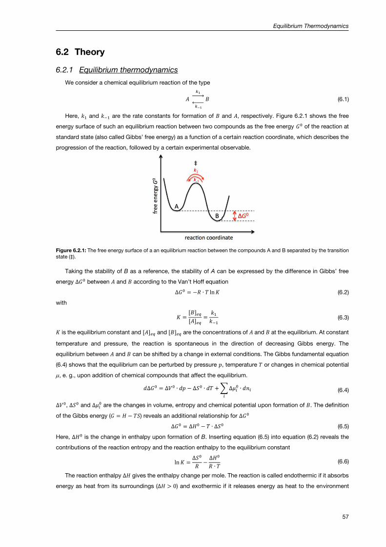
Equilibrium Thermodynamics
57
6.2 Theory
6.2.1 Equilibrium thermodynamics
We consider a chemical equilibrium reaction of the type
𝐴
𝑘1 →
𝑘−1 ←
𝐵 (6.1)
Here, 𝑘1 and 𝑘−1 are the rate constants for formation of 𝐵 and 𝐴, respectively. Figure 6.2.1 shows the free
energy surface of such an equilibrium reaction between two compounds as the free energy 𝐺0 of the reaction at
standard state (also called Gibbs’ free energy) as a function of a certain reaction coordinate, which describes the
progression of the reaction, followed by a certain experimental observable.
Figure 6.2.1: The free energy surface of a an equilibrium reaction between the compounds A and B separated by the transition state (‡).
Taking the stability of B as a reference, the stability of A can be expressed by the difference in Gibbs’ free
energy ∆𝐺0 between 𝐴 and 𝐵 according to the Van’t Hoff equation
∆𝐺0 = −𝑅 ∙ 𝑇 ln𝐾 (6.2)
with
𝐾 =[𝐵]𝑒𝑞
[𝐴]𝑒𝑞=
𝑘1𝑘−1
(6.3)
𝐾 is the equilibrium constant and [𝐴]𝑒𝑞 and [𝐵]𝑒𝑞 are the concentrations of 𝐴 and 𝐵 at the equilibrium. At constant
temperature and pressure, the reaction is spontaneous in the direction of decreasing Gibbs energy. The
equilibrium between 𝐴 and 𝐵 can be shifted by a change in external conditions. The Gibbs fundamental equation
(6.4) shows that the equilibrium can be perturbed by pressure 𝑝, temperature 𝑇 or changes in chemical potential
, e. g., upon addition of chemical compounds that affect the equilibrium.
𝑑∆𝐺0 = ∆𝑉0 ∙ 𝑑𝑝 − ∆𝑆0 ∙ 𝑑𝑇 +∑∆𝜇𝑖0 ∙ 𝑑𝑛𝑖
𝑖
(6.4)
∆𝑉0, ∆𝑆0 and ∆𝜇𝑖0 are the changes in volume, entropy and chemical potential upon formation of 𝐵. The definition
of the Gibbs energy (𝐺 = 𝐻 − 𝑇𝑆) reveals an additional relationship for ∆𝐺0
∆𝐺0 = ∆𝐻0 − 𝑇 ∙ ∆𝑆0 (6.5)
Here, ∆𝐻0 is the change in enthalpy upon formation of B. Inserting equation (6.5) into equation (6.2) reveals the
contributions of the reaction entropy and the reaction enthalpy to the equilibrium constant
ln 𝐾 =∆𝑆0
𝑅−∆𝐻0
𝑅 ∙ 𝑇 (6.6)
The reaction enthalpy ∆𝐻 gives the enthalpy change per mole. The reaction is called endothermic if it absorbs
energy as heat from its surroundings (∆𝐻 > 0) and exothermic if it releases energy as heat to the environment

Equilibrium Thermodynamics
58
(∆𝐻 < 0). The superscript zero further indicates that all species involved in the reaction are in their standard states,
namely in their pure form at a pressure 𝑝 = 1 bar at a specified temperature. The standard enthalpy may thus be
reported for any temperature. The conventional temperature for reporting thermodynamic data is 298.15 K (25C).
6.2.2 Effect of temperature on an equilibrium reaction
Changing the temperature perturbs the equilibrium resulting in a new equilibrium with different concentrations
of 𝐴 and 𝐵. The principle of Le Chatelier predicts that the system at equilibrium readjusts itself to counteract the
effect of the applied change. Regarding the effect of changing the temperature on a chemical equilibrium, this
means that: i) the equilibrium will shift in the endothermic direction if the temperature is raised, because then
energy is absorbed as heat and the rise in temperature is opposed and ii) the equilibrium will shift in the exothermic
direction if the temperature is lowered, because then energy is released and the reduction in temperature is
opposed. This can be can be summarized in the following way:
- Exothermic reactions: increasing the temperature favours the reactants.
- Endothermic reactions: increasing the temperature favours the products.
Writing the expression ∆𝐺 = ∆𝐻 − 𝑇 ∙ ∆𝑆 in the form −∆𝐺 𝑇⁄ = −∆𝐻 𝑇⁄ + ∆𝑆 reveals some insight into the
thermodynamic basis of this behaviour. For an exothermic reaction, −∆𝐻 𝑇⁄ corresponds to a positive change of
entropy of the surroundings and favours the formation of products. When the temperature is raised, −∆𝐻 𝑇⁄
decreases, and the increasing entropy of the surroundings has a less important role. As a result, the equilibrium
shifts to the left. For an endothermic reaction, the principal factor is the increasing entropy of the reaction system.
The importance of the unfavourable change of entropy of the surroundings is reduced if the temperature is raised
(because then −∆𝐻 𝑇⁄ is smaller), and the reaction is able to shift towards the products. Quantitatively, this is
described by equation (6.6). According to this equation, a plot of ln 𝐾 versus 1/𝑇 (Van’t Hoff plot) yields a straight
line with the slope
𝑚 = −∆𝐻0 𝑅⁄ and the intercept 𝑏 = ∆𝑆0 𝑅⁄ . Thus, it is quite easy to determine ∆𝐻0 and ∆𝑆0 graphically. However,
it has to be taken into account that the reaction enthalpy and the reaction entropy are dependent on temperature
due to changes in heat capacity ∆𝐶𝑝 with temperature (for the meaning of the heat capacity also see chapter 4).
∆𝐶𝑝 ≠ 0 leads to a curved line in the Van’t Hoff plot. However, if the investigated temperature range is small and
the temperature dependence of the heat capacity small, then a straight line can be assumed. Usually, the method
of using Van’t Hoff plot is accurately enough to determine the reaction enthalpy and the reaction entropy.
6.2.3 Absorption spectroscopy
In this experiment, an equilibrium reaction is investigated using UV-Vis absorption spectroscopy. All optical
spectroscopic methods are based on the basic principle that electromagnetic radiation is irradiated to the object
under investigation and it is absorbed, scattered and again emitted. As its name already reveals, UV-Vis
absorption spectroscopy uses the absorption of light in the UV-Vis range (100 nm - 760 nm). A prerequisite for
light absorption is the presence of a chromophor, which is the part of a molecule that is responsible for light
absorption due to its electronic transitions. The possible electronic transitions (mainly *, n* and n*) are
excited by light absorption and together with their rotational and vibrational levels they lead to the specific shape
(position, width and intensity of spectral lines) of the absorption spectrum.
The Lambert-Beer law (equation (6.7)) quantitatively describes the absorption of electromagnetic radiation by
a substance in solution. This law assumes that the absorbing substance is homogenously distributed, that no light
scattering occurs and that no other photoreactions are taking place in the solution. The absorbance 𝐴 of

Equilibrium Thermodynamics
59
monochromatic light (meaning with a given wavelength , and thus with a given energy) by a solved substance is
then given by
𝐴 = log𝐼0𝐼= 휀 ∙ 𝑐 ∙ 𝑑 (6.7)
Here, 𝐼0 and 𝐼 are the intensity of the irradiated light and of the light leaving the sample, respectively. 𝑐 is the
molar concentration of the light absorbing substance, 𝑑 is the thickness of the irradiated sample in cm and is
the substance-specific molar absorption coefficient in M-1 cm-1. If the substance under investigation absorbs light
in the used wavelength range, equation (6.7) can thus be used to determine its concentration. Instead of the
absorbance 𝐴, the transmittance 𝑇 is often used to quantify the effect of light absorption. Both parameters are
directly related
𝑇 =𝐼
𝐼0 (6.8)
and thus
𝐴 = − log 𝑇 (6.9)
According to Lambert-Beer law (equation (6.7)), an absorption spectrum is a plot of the extinction coefficient as
a function of the wavelength of the irradiated light. Note that the shape of the spectrum further depends strongly
on the solvent due to interactions of the substance with the solvent dipoles, due to collisions with solvent
molecules and possibly also due to hydrogen bond formation.
Two major devices are used to perform spectrophotometric measurements. Using single-beam
spectrophotometers like in this experiment, the sample and the reference have to be measured separately. In
contrast to this, double-beam spectrophotometers (Figure 6.2.2) compare the light intensity between two light
paths, one path containing a reference sample and the other a test sample. The reference and the sample are
measured alternately using a chopper mirror that switches the light from one optical path to the other.
Figure 6.2.2: Setup of a dual beam spectrophotometer.
6.2.4 The reaction of Rhodamine B
In this experiment, the parameters ∆𝐺0, ∆𝐻0 and ∆𝑆0 of an equilibrium reaction are determined using
spectrophotometry. Here, the chemical dye Rhodamine B chloride is used. In solution Rhodamine B chloride is
present as equilibrium of two different structures (Figure 6.2.3). On one hand there is the colourless lactone form
(L) of Rhodamine B and on the other hand there is the chromatic zwitterionic form (Z) of Rhodamide B. Increasing
the temperature favours the colourless lactone form.
Do you know why the lactone is colourless while the zwitterion is coloured?

Equilibrium Thermodynamics
60
Figure 6.2.3: Equilibrium structures (left: lactone, right: zwitterion) of Rhodamin B in solution.
Since the lactone is colourless and the zwitterion is chromatic, the equilibrium concentrations can be
determined using UV-Vis absorption spectroscopy. Knowing the equilibrium concentrations allows calculation of
the equilibrium constant 𝐾 = [𝑍]/[𝐿]. In order to be able to determine 𝐾 as a function of temperature, the
absorbance of the pure Z-form needs to be known. This value can be determined from measurements of
Rhodamin B chloride in strong acids. However, this is not part of this experiment and the corresponding value of
the molar absorption coefficient of the pure Z-form ( = 13.0104 M-1 cm-1) is provided.
6.3 Experimental details and evaluation
6.3.1 Experimental execution
Aim of the experiment is the determination of ΔG0, ΔH0 und ΔS0 for formation of the zwitterion form of
Rhodamine B either in ethanol or in 1-propanol. The two Rhodamin B solutions A and B are provided at the bench:
Solution A: 8∙10-6 M Rhodamin B in ethanol
Solution B: 8∙10-6 M Rhodamin B in 1-propanol
The students may decide themselves, which solution they want to start with. Figure 6.3.1 shows the single beam
spectrophotometer used to characterize the equilibrium reaction under investigation.
Figure 6.3.1: Spectrophotometer used to study the equilibrium reaction of Rhodamine B.
Before the measurements on the Rhodamine-B solutions can be performed, the spectrophotometer needs to be
calibrated by making a base correction. This has to be done for each series of measurement individually, meaning
once before the measurements in the first solvent and once before the measurements in the second alcohol.
Check if the provided cuvettes are clean and dry. In order to perform the base correction, fill one cuvette with the

Equilibrium Thermodynamics
61
corresponding pure alcohol and place it in the cuvette holder equilibrated to 𝑇 = 25 C and close the sample
chamber. The temperature can be adjusted by setting the temperature controller.
Figure 6.3.2: Controller for the temperature adjustment of the cell holder.
To adjust the requested temperature set the switch “TEMP. CONTROL” to “OFF”. Turn the knob labelled
“TEMP.ADJUSTMENT” to the left (“DOWN”) to decrease, or to the right (“UP”) to increase the temperature of the
temperature controlled cell holder. Then set the switch “TEMP. CONTROL” to “ON”.
Figure 6.3.3: The temperature controlled cell holder.
In “Mode menu” (Figure 6.3.4) select “Spectrum” to change to the “Spectrum menu” and start the base correction
“BaseCorr” (Figure 6.3.5) by pressing F1.
Figure 6.3.4: The “MODE menu”.

Equilibrium Thermodynamics
62
Figure 6.3.5: The “Spectrum menu”; press F1 (“BaseCorr”) to start the base correction.
When the measurement is finished, empty the cuvette into the waste can for “Halogenfreie Lösungsmittel”.
Clean and dry the cuvette as described above and fill it with the corresponding Rhodamine B solution. Put the
cuvette in the cuvette holder. Cover the cuvette with the insulator cap equipped with the thermocouple and close
the sample chamber. Take care of the Ni- Cr/Ni temperature sensor!
Think about why it is important to close the cuvettes. What would happen if the cuvettes were open? What
would be the consequences of that?
In a first step the students determine the wavelength (max) of maximum absorbance for the corresponding
Rhodamine B solution. To perform this, the students have to measure three absorbance spectra of the Rhodamine
B solution in the range from 450 nm to 600 nm at three different temperatures (15, 25 and 40 °C). To start the
measurement just press the START/STOP button and a spectrum like in Figure 6.3.7 will appear. In order to obtain
the wavelength of maximum absorbance press F2 (PEAK button).
Figure 6.3.6: The keyboard of the single beam spectrometer.
In the following measurements, the absorbance at the wavelength of its maximum in determined as a function
of temperature. To perform these measurements, go back to the “Mode menu” (Figure 6.3.4) of the spectrometer
and choose "Photometric". Adjust the wavelength to the determined maximum of absorbance. Heat the cuvette
to 𝑇 = 60 °C and measure the absorbance spectrum by pressing the “START/STOP”-button (Figure 6.3.6). If the
set temperature of 𝑇 = 60 °C is reached and the corresponding absorbance is written down, the temperature
should be then set to 𝑇 = 10 °C. Because of this, the solution in the cuvette starts cooling down. Follow the actual
temperature in the cuvette on the computer display and read the temperature in maximum steps of ∆𝑇 = 5 °C
down to T = 15 °C. For each temperature value press the “START/STOP”-button and determine the actual
absorbance value! Please collect the series of measurement going from high to low temperature for three times
for each Rhodamine B solution, in order to get enough values to estimate the error. The thereby collected
absorbance values are stored in a table (Figure 6.3.8) in the spectrometer software.

Equilibrium Thermodynamics
63
Figure 6.3.7: In the “Spectrum menu”, press F2 (“Peak”) to get the wavelength of maximum absorbance.
Figure 6.3.8: The table with the stored absorbance values.
Right after collecting the absorbance values, you should manually fill it in the prepared spreadsheet (similarly
to Table 6.1.1)
After emptying and cleaning all cuvettes, repeat the measurements for the second Rhodamine-B solution.
6.3.2 Data evaluation
Determine the concentration of the zwitterion form of Rhodamine B as a function of temperature, using
Lambert-Beer law. For this, it is necessary to calculate the absorbance 𝐴(100%) of the pure Z-form,
meaning that all Rhodamine B is present in its zwitterion form using the given molar extinction coefficient.
The concentration of the zwitterion form at a certain temperature is then given by
[𝑍] =𝐴(𝑇) ⋅ 𝜌(15 °𝐶)
𝐴(100%) ⋅ 𝜌(𝑇) (6.10)
where 𝜌(15 °𝐶) is the density of the solvent at 15 °C and 𝜌(𝑇) the density of the solvent at the measuring
temperature 𝑇. 𝐴(𝑇) is the absorbance at the measuring temperature. Values for the density of the used
solvents are provided in the lab. The temperature dependence of the density can be assumed to be
linear.
Use the relation [L] = 1 – [Z] to determine the equilibrium constant according to equation (6.3) for all
the measurements and for both Rhodamine B solutions.
Determine ΔG0, ΔH0 und ΔS0 for the formation of the zwitterion form of Rhodamine B in both solvents.
Discuss the size and the sign of the results. Why does the equilibrium move to the lactone form with
increasing temperature?
Perform an error analysis for all calculations.

Equilibrium Thermodynamics
64
6.4 Applications of the experiment and its theory
In quantitative analyses of molecules that absorb light in the UV-Vis range of the electromagnetic
spectrum, their concentration can be determined by absorption spectroscopy. Furthermore, this allows
to derive equilibrium constants, dissociation constants and reaction kinetics.
Since the absorption spectrum is specific for each compound, its measurement allows identification
and purity analysis of molecules in solution.
UV-Vis absorption spectroscopy allows trace analysis, e. g., determination of the ethanol concentration
in the blood.
Rhodamine dyes are widely used as fluorescent probes, owing to their high absorption and broad
fluorescence in the visible region of the electromagnetic spectrum [6.4].
Equilibrium reactions are ubiquitous in chemistry and in biology, some examples are: saturated
solutions above a precipitate (e.g., 𝐴𝑔+ + 𝐶𝑙− ⇆ 𝐴𝑔𝐶𝑙), ester formation from acid and alcohol, phase
equilibria, formation of crystals and flowstones, etc.. The analysis of the corresponding equilibrium
thermodynamics is important for characterization and understanding of these systems [6.5, 6.6].
6.5 Literature
6.1 - D.A. Hinkley and P.G. Seybold, J. Chem. Education, 64, (1987) 382-384.
6.2 - P.W. Atkins, Physical Chemistry, 6th ed., Oxford University Press, Oxford (1998), pp. 215-242.
6.3 - P.W. Atkins and J. de Paula, Atkins’ Physical Chemistry, 8th ed., Oxford University Press, Oxford (2006),
pp. 200-215.
6.4 - Beija, M., Afonso C.A.M., and Martinho J.M.G., Synthesis and applications of Rhodamine derivatives as
fluorescent probes, Chem. Soc. Rev., 38 (2009) 2410-2433.
6.5 - L. Stixrude and C. Lithgow-Bertelloni, Thermodynamics of mantle minerals, Geophysical Journal
international, 184 (2011) 1180-1213.
6.6 - K. Sakurai, M. Oobatake and Y. Goto, Salt-dependent monomer-dimer equilibrium of bovine -lactoglobulin
at pH 3, Protein Science, 10 (2001) 2325-2335.
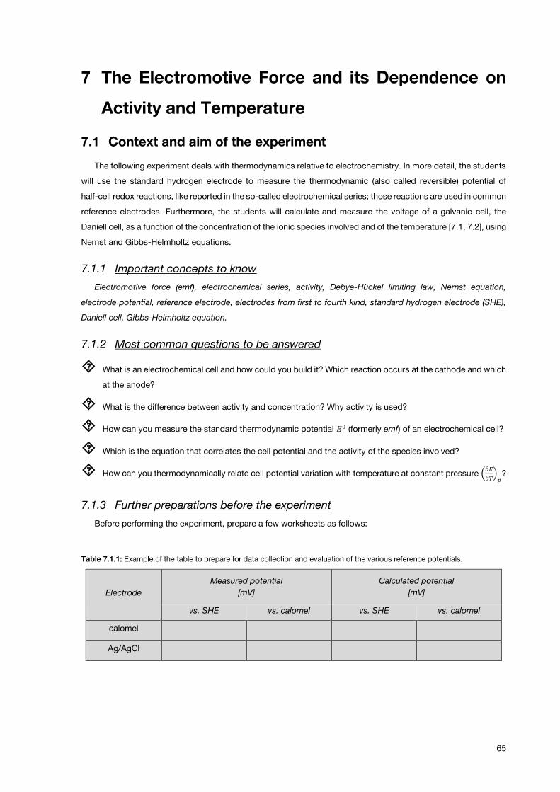
65
7 The Electromotive Force and its Dependence on
Activity and Temperature
7.1 Context and aim of the experiment
The following experiment deals with thermodynamics relative to electrochemistry. In more detail, the students
will use the standard hydrogen electrode to measure the thermodynamic (also called reversible) potential of
half-cell redox reactions, like reported in the so-called electrochemical series; those reactions are used in common
reference electrodes. Furthermore, the students will calculate and measure the voltage of a galvanic cell, the
Daniell cell, as a function of the concentration of the ionic species involved and of the temperature [7.1, 7.2], using
Nernst and Gibbs-Helmholtz equations.
7.1.1 Important concepts to know
Electromotive force (emf), electrochemical series, activity, Debye-Hückel limiting law, Nernst equation,
electrode potential, reference electrode, electrodes from first to fourth kind, standard hydrogen electrode (SHE),
Daniell cell, Gibbs-Helmholtz equation.
7.1.2 Most common questions to be answered
What is an electrochemical cell and how could you build it? Which reaction occurs at the cathode and which
at the anode?
What is the difference between activity and concentration? Why activity is used?
How can you measure the standard thermodynamic potential 𝐸0 (formerly emf) of an electrochemical cell?
Which is the equation that correlates the cell potential and the activity of the species involved?
How can you thermodynamically relate cell potential variation with temperature at constant pressure (𝜕𝐸
𝜕𝑇)𝑝?
7.1.3 Further preparations before the experiment
Before performing the experiment, prepare a few worksheets as follows:
Table 7.1.1: Example of the table to prepare for data collection and evaluation of the various reference potentials.
Electrode
Measured potential
[mV]
Calculated potential
[mV]
vs. SHE vs. calomel vs. SHE vs. calomel
calomel
Ag/AgCl

The Electromotive Force and its Dependence on Activity and Temperature
66
Table 7.1.2: Example of the table to prepare for data collection and evaluation of the voltage of the Daniell cell as a function of concentration of ionic species.
Daniell cell
Measured
potential
[mV]
Calculated
potential
[mV]
ln 𝑎𝑍𝑛2+ 𝑎𝐶𝑢2+⁄
… … …
Table 7.1.3: Example of the table to prepare for data collection and evaluation of the voltage of the Daniell cell as a function of temperature.
Daniell cell
Potential
[mV]
Temperature
[K]
… …
… …
… …
7.2 Theory
7.2.1 Activity and concentration
In concentrated solutions, the strong interactions of the dissolved ionic species with each other, not only with
the solvent, become relevant. In order to use real solutions and be able to physically model them, the
concentration 𝑏𝑖 in mol/kg (molality) of a dissolved species 𝑖 must be replaced with a “thermodynamically effective
quantity” 𝑎𝑖, denominated activity. This physical quantity is dimensionless and it is obtained by dividing the
molality 𝑏𝑖 of the species 𝑖 by the standard molality 𝑏0 = 1 mol/kg. The relationship between concentration and
activity is then
𝑎𝑖 = 𝛾𝑖 ∙𝑏𝑖𝑏0 (with lim
𝑏𝑖→0𝛾𝑖 = 1) (7.1)
where 𝑏𝑖 is the concentration in mol/kg of a dissolved species 𝑖 and 𝛾𝑖 is its activity coefficient.
In the case of a solution of an salt, the physico-chemical methods refer constantly to the mean ionic activity
𝑎𝑖±, since both ions need to be dissolved to fulfil electroneutrality of the solution. The mean ionic activity of an
electrolyte is defined as the geometric mean of the ion activities
𝑎𝑖± = (𝑎𝑖+𝜈+ ∙ 𝑎𝑖−
𝜈−)1𝜈 (7.2)
where 𝜈+ and 𝜈−are the amounts of positive and negative ions resulting from the dissociation of one formula unit
of the salt and 𝜈 = 𝜈+ + 𝜈− . For example, for NaCl 𝑎𝐻𝐶𝑙± = (𝑎𝐻+ ∙ 𝑎𝐶𝑙−)1
2.
Using the mean ionic activity coefficient 𝛾𝑖±, defined similarly to the mean ionic activity, it results
𝑎𝑖± = 𝛾𝑖± ∙𝑏𝑖𝑏0
(7.3)
According to the Debye-Hückel limiting law [7.1, 7.3], valid for diluted solutions (< 10-3 mol/kg) results
log10 𝛾𝑖± = −0.509 ∙ |𝑧𝑖+ ∙ 𝑧𝑖−| ∙ √𝐼 (7.4)
where 𝑇 = 298 𝐾, 𝑏𝑖 → 0, 𝑧𝑖+ and 𝑧𝑖− are the charges of the positive and negative ions. The dimensionless ionic
strength 𝐼 is defined as
𝐼 =1
2∙∑
𝑏𝑖𝑏0
∙ 𝑧𝑖2
𝑖
(7.5)
where 𝑏𝑖 is the concentration in mol/kg of each ionic species 𝑖, 𝑧𝑖 is the charge of each dissolved ionic species
and 𝛴𝑖 is the sum over all the ionic species 𝑖. Table 7.2.1 reports some examples on how to calculate the ionic

The Electromotive Force and its Dependence on Activity and Temperature
67
strengths of 1 mol/kg solutions for various salts. The activity of a solid, e. g., insoluble salts or pure metals, is
defined as 1.
Table 7.2.1: Examples of ionic-strength calculations of 1 mol/kg solutions of various salts.
Type of salt 𝐼 Type of salt 𝐼
1, 1 (NaCl) 1
2(1 ∙ 1² + 1 ∙ 1²) = 1 1, 3 (LaCl3)
1
2(1 ∙ 3² + 3 ∙ 1²) = 6
1, 2 (BaCl2) 1
2(1 ∙ 2² + 2 ∙ 1²) = 3 1, 3 (K3PO4)
1
2(3 ∙ 1² + 1 ∙ 3²) = 6
2, 2 (ZnSO4) 1
2(1 ∙ 2² + 1 ∙ 2²) = 4 2, 3 (Mg3(PO4)2)
1
2(3 ∙ 2² + 2 ∙ 3²) = 15
In the case of solutions having a concentration higher than 10-3 mol/kg (too high ionic strength) the
Debye-Hückel limiting law is not fitting the real trend anymore and the activity coefficients can be estimated using
a semi-empirical fit of that law, called extended Debye-Hückel law
log10 𝛾𝑖± = −A ∙ |𝑧𝑖+ ∙ 𝑧𝑖−| ∙ √𝐼
1 + B ∙ √𝐼+ 𝐶 ∙ 𝐼 (7.6)
where A, B and 𝐶 are adjustable empiric parameters characteristic of each salt. This equation is also fitting the
real value only for concentration lower than 0.1 mol/kg. For higher concentrations, there is no widely accepted
model and the values are determined experimentally or with the use of thermodynamic state functions.
7.2.2 Electrochemical cells and emf
An electrochemical cell consists of two electrodes, which must conduct electrons, in contact with an ionic
conductive medium (electrolyte). If the two electrodes are in different compartments, an ionic contact between
the compartments (salt bridge) is needed to run the cell. An electrochemical cell is called galvanic if its overall
electrochemical reaction is spontaneous (exergonic, ∆𝐺 < 0); in this case, an electronic current will flow between
the electrodes, if they are in electric contact, and, at the same time, an ionic current will flow through the
electrolyte, to avoid separation of ionic charges because of the ionic species produced. On the opposite, an
electrochemical cell is called electrolytic if its overall electrochemical reaction is non-spontaneous (endergonic,
∆𝐺 > 0); in this case, the reaction happens only if a power supply provides enough electric work (electric current
between the two electrodes) for the electrochemical reaction to occur.
At each electrode, a half-cell reaction occurs with a transfer of electrons, also called redox reaction. If electrons
are flowing to an electrode, there a reduction reaction happens and the electrode is called cathode (equation
(7.7)). The electrons flowing to the cathode must come from the other electrode, where an oxidation reaction must
occur; this electrode is called anode (equation (7.8)). Using the common sign convention, the cathode is the
positive electrode in a galvanic cell and the negative electrode in an electrolytic cell, while for the anode the signs
are the opposite.
Cathode: Galvanic cell: Electrolytic cell:
𝑂𝑥1 + 𝑛𝑒− ⇄ 𝑅𝑒𝑑1 (7.7)
Anode: Galvanic cell: Electrolytic cell:
𝑅𝑒𝑑2 ⇄ 𝑂𝑥2 + 𝑛𝑒− (7.8)
𝑂𝑥1 + 𝑅𝑒𝑑2 ⇄ 𝑅𝑒𝑑1 + 𝑂𝑥2 (7.9)

The Electromotive Force and its Dependence on Activity and Temperature
68
If the two electrodes are not in electric contact, only the dynamic equilibria of the single half-cells are active
and no change will occur; this condition is called open circuit. If the two half-cell reactions are not in equilibrium,
as soon as the circuit is closed (i. e., the two electrodes are in electric contact and electrons are flowing) the
electrochemical cell can provide an electric work 𝑤𝑒. This quantity is related to the difference in (electrochemical)
potential between the two electrodes, called cell voltage, measured in volts (V). The maximum possible electric
work 𝑤𝑒𝑚𝑎𝑥 that the cell can perform in fully reversible conditions is the Gibbs free energy ∆𝐺𝑝,𝑇 at constant
pressure and temperature. This is directly related to the cell potential when zero current is flowing through the
circuit, that is called thermodynamic or reversible cell potential 𝐸, formerly electromotive force 𝑒𝑚𝑓. This quantity
is measured using a voltmeter at open circuit, and is practically called open-circuit voltage (OCV) of the particular
electrochemical cell.
7.2.3 Thermodynamic Cell Potential and Nernst Equation
The relation between the thermodynamic cell potential 𝐸 and the Gibbs free energy ∆𝐺 is:
∆𝐺 = −𝑛 ∙ 𝐹 ∙ 𝐸 (7.10)
where 𝑛 is the number of electrons exchanged in the electrochemical reaction (equations (7.7) and (7.8)) and 𝐹 is
the Faraday constant (product of the charge of electron 𝑒 and the Avogadro number 𝑁𝐴, 𝐹 = 96485 𝑘𝐶/𝑚𝑜𝑙). From
the sign in the equation it is easy to infer that 𝐸 is positive if the ∆𝐺 is negative (spontaneous reaction) and vice
versa.
It is known that the Gibbs free energy is related to the reaction-mixture composition by
∆𝐺 = ∆𝐺0 + 𝑅 ∙ 𝑇 ∙ ln∏𝑎𝑖𝜈𝑖
𝑖
(7.11)
where 𝑅 is the ideal-gas constant, 𝑇 is the temperature and 𝑎𝑖 is the activity of each term 𝑖 of a chemical reaction
elevated to its stoichiometric coefficient 𝜈𝑖 (negative for the reactants). Dividing both sides by – 𝑛𝐹 and using
equation (7.10), it results that:
𝐸 = −∆𝐺0
𝑛 ∙ 𝐹−𝑅 ∙ 𝑇
𝑛 ∙ 𝐹∙ ln∏𝑎𝑖
𝜈𝑖
𝑖
(7.12)
Using equation (7.10), the first term on the right of equation (7.12) can be defined as the standard thermodynamic
cell potential 𝐸0 (at 𝑇 = 298.15 K, 𝑝 = 1 atm and 𝑎𝑖 = 1). Thus we can write
𝐸 = 𝐸0 −𝑅 ∙ 𝑇
𝑛 ∙ 𝐹∙ ln∏𝑎𝑖
𝜈𝑖
𝑖
(7.13)
and equation (7.13) is called Nernst equation.
The term ∏ 𝑎𝑖𝜈𝑖
𝑖 is also called reaction quotient and it is calculated using the activities 𝑎𝑖 at zero current, i. e.,
before letting the electrons flow through the circuit. Of course, after the electrochemical reaction reaches its
equilibrium, its thermodynamic cell potential is zero, exactly like its Gibbs free energy.
7.2.4 Half-cell potentials, standard potentials and reference electrodes
It is practically a nonsense to think to measure the single potential of only one electrode reaction (half-cell
potential) completely separated from a second electrode or, in other words, everything is relative. Nevertheless,
it is possible to measure the potential difference of every possible electrode reaction relatively to another, which
is characterized by a well-defined potential, called standard potential similarly to all the standard conditions used
to define the value of the Gibbs free energy of a reaction.
The well-known electrode used as standard to measure the potential of others is the standard hydrogen
electrode (SHE). It is an electrode of the fourth kind, i.e. consists of an inert metal (Pt) in the presence of H2 gas
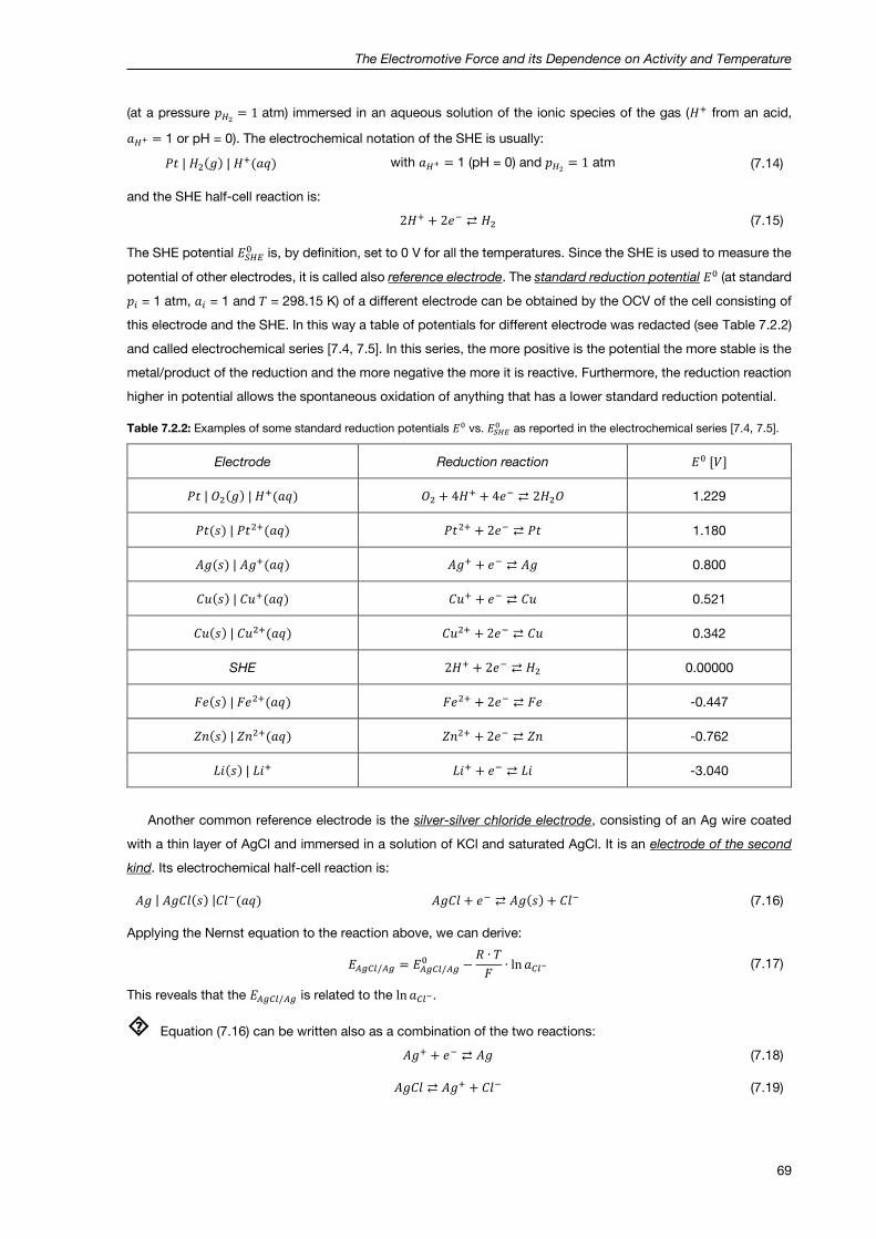
The Electromotive Force and its Dependence on Activity and Temperature
69
(at a pressure 𝑝𝐻2 = 1 atm) immersed in an aqueous solution of the ionic species of the gas (𝐻+ from an acid,
𝑎𝐻+ = 1 or pH = 0). The electrochemical notation of the SHE is usually:
𝑃𝑡 | 𝐻2(𝑔) | 𝐻+(𝑎𝑞) with 𝑎𝐻+ = 1 (pH = 0) and 𝑝𝐻2 = 1 atm (7.14)
and the SHE half-cell reaction is:
2𝐻+ + 2𝑒− ⇄ 𝐻2 (7.15)
The SHE potential 𝐸𝑆𝐻𝐸0 is, by definition, set to 0 V for all the temperatures. Since the SHE is used to measure the
potential of other electrodes, it is called also reference electrode. The standard reduction potential 𝐸0 (at standard
𝑝𝑖 = 1 atm, 𝑎𝑖 = 1 and 𝑇 = 298.15 K) of a different electrode can be obtained by the OCV of the cell consisting of
this electrode and the SHE. In this way a table of potentials for different electrode was redacted (see Table 7.2.2)
and called electrochemical series [7.4, 7.5]. In this series, the more positive is the potential the more stable is the
metal/product of the reduction and the more negative the more it is reactive. Furthermore, the reduction reaction
higher in potential allows the spontaneous oxidation of anything that has a lower standard reduction potential.
Table 7.2.2: Examples of some standard reduction potentials 𝐸0 vs. 𝐸𝑆𝐻𝐸0 as reported in the electrochemical series [7.4, 7.5].
Electrode Reduction reaction 𝐸0 [𝑉]
𝑃𝑡 | 𝑂2(𝑔) | 𝐻+(𝑎𝑞) 𝑂2 + 4𝐻+ + 4𝑒− ⇄ 2𝐻2𝑂 1.229
𝑃𝑡(𝑠) | 𝑃𝑡2+(𝑎𝑞) 𝑃𝑡2+ + 2𝑒− ⇄ 𝑃𝑡 1.180
𝐴𝑔(𝑠) | 𝐴𝑔+(𝑎𝑞) 𝐴𝑔+ + 𝑒− ⇄ 𝐴𝑔 0.800
𝐶𝑢(𝑠) | 𝐶𝑢+(𝑎𝑞) 𝐶𝑢+ + 𝑒− ⇄ 𝐶𝑢 0.521
𝐶𝑢(𝑠) | 𝐶𝑢2+(𝑎𝑞) 𝐶𝑢2+ + 2𝑒− ⇄ 𝐶𝑢 0.342
SHE 2𝐻+ + 2𝑒− ⇄ 𝐻2 0.00000
𝐹𝑒(𝑠) | 𝐹𝑒2+(𝑎𝑞) 𝐹𝑒2+ + 2𝑒− ⇄ 𝐹𝑒 -0.447
𝑍𝑛(𝑠) | 𝑍𝑛2+(𝑎𝑞) 𝑍𝑛2+ + 2𝑒− ⇄ 𝑍𝑛 -0.762
𝐿𝑖(𝑠) | 𝐿𝑖+ 𝐿𝑖+ + 𝑒− ⇄ 𝐿𝑖 -3.040
Another common reference electrode is the silver-silver chloride electrode, consisting of an Ag wire coated
with a thin layer of AgCl and immersed in a solution of KCl and saturated AgCl. It is an electrode of the second
kind. Its electrochemical half-cell reaction is:
𝐴𝑔 | 𝐴𝑔𝐶𝑙(𝑠) |𝐶𝑙−(𝑎𝑞) 𝐴𝑔𝐶𝑙 + 𝑒− ⇄ 𝐴𝑔(𝑠) + 𝐶𝑙− (7.16)
Applying the Nernst equation to the reaction above, we can derive:
𝐸𝐴𝑔𝐶𝑙/𝐴𝑔 = 𝐸𝐴𝑔𝐶𝑙/𝐴𝑔0 −
𝑅 ∙ 𝑇
𝐹∙ ln 𝑎𝐶𝑙− (7.17)
This reveals that the 𝐸𝐴𝑔𝐶𝑙/𝐴𝑔 is related to the ln 𝑎𝐶𝑙−.
Equation (7.16) can be written also as a combination of the two reactions:
𝐴𝑔+ + 𝑒− ⇄ 𝐴𝑔 (7.18)
𝐴𝑔𝐶𝑙 ⇄ 𝐴𝑔+ + 𝐶𝑙− (7.19)

The Electromotive Force and its Dependence on Activity and Temperature
70
The derivation of Equation (7.17) from the Nernst equation of reaction (7.18) and the solubility equilibrium of
reaction (7.19) is left to the student.
An electrode of the third kind is an inert metal in a solution of two redox species of the same element.
A further common reference electrode is the calomel electrode, consisting of a Pt wire in electric contact with
liquid mercury and mercury (I) chloride (calomel, Hg2Cl2) which, in turn, are in contact with a saturated solution of
KCl in water. The electrochemical half-cell reaction is:
𝑃𝑡 | 𝐻𝑔(𝑠) |𝐻𝑔2𝐶𝑙2(𝑠) | 𝐶𝑙−(𝑎𝑞) 𝐻𝑔2𝐶𝑙2(𝑠) + 2𝑒− ⇄ 2𝐻𝑔(𝑠) + 2𝐶𝑙− (7.20)
Applying the Nernst equation to the reaction above, we can derive:
𝐸𝐻𝑔2𝐶𝑙2/𝐻𝑔 = 𝐸𝐻𝑔2𝐶𝑙2/𝐻𝑔0 −
𝑅 ∙ 𝑇
2𝐹∙ ln 𝑎𝐶𝑙−
2 = 𝐸𝐻𝑔2𝐶𝑙2/𝐻𝑔0 −
𝑅 ∙ 𝑇
𝐹∙ ln 𝑎𝐶𝑙− (7.21)
7.2.5 The Daniell cell and its temperature dependence
The Daniell cell is a well-known example of electrochemical galvanic cell. It is composed by a metallic zinc
electrode immersed in a solution of Zn(II) sulfate and a metallic copper electrode immersed in a solution of Cu(II)
sulfate. The two half-cells are put in ionic contact between each other using a salt bridge (which contains a salt
solution) or an ionic conductive membrane. The cell can be schematized as follows:
𝑍𝑛(𝑠) | 𝑍𝑛𝑆𝑂4(𝑎𝑞) || 𝐶𝑢𝑆𝑂4(𝑎𝑞) | 𝐶𝑢(𝑠) (7.22)
The half-cell electrodes here are electrodes of the first kind.
To understand at which electrode the reduction and at which the oxidation can happen spontaneously, one can
think that the reduction reaction with the higher standard potential takes place at the cathode. From Table 7.2.2
it is evident that the cathode is the Cu electrode while the anode is the Zn, for a spontaneous electrochemical
reaction. This means that, if the two electrodes are in electric contact, zinc dissolves while copper deposits as
metal on the cathode and electrons spontaneously flow from Zn to Cu. If the electrodes are not in electric contact,
the following equilibrium reactions occur:
Cathode: 𝐶𝑢2+ + 2𝑒− ⇄ 𝐶𝑢 (7.23)
Anode: 𝑍𝑛 ⇄ 𝑍𝑛2+ + 2𝑒− (7.24)
𝐶𝑢2+ + 𝑍𝑛 ⇄ 𝐶𝑢 + 𝑍𝑛2+ (7.25)
The standard thermodynamic potential of the galvanic cell 𝐸0 is the difference between the standard reduction
potential of the cathode and that of the anode, 𝐸0 = 𝐸𝑐 − 𝐸𝑎, and can be calculated from Table 7.2.2. For the
overall electrochemical reaction (7.25) the cell potential can be calculated using the Nernst equation to be
𝐸 = 𝐸0 −𝑅 ∙ 𝑇
2 ∙ 𝐹∙ ln
𝑎𝑍𝑛2+ ∙ 𝑎𝐶𝑢𝑎𝐶𝑢2+ ∙ 𝑎𝑍𝑛
(7.26)
The measurement of the cell potential can be performed with voltmeters, characterized by a high internal electrical
resistance and designed to measure a voltage difference between two electrodes with a negligible current flow
between them, thus with negligible perturbation, obtaining real values of the OCV (open-circuit voltage).
The temperature dependence of the cell potential is evident in the second term of equation (7.26). Furthermore,
also the standard thermodynamic potential of the galvanic cell 𝐸0 has an intrinsic temperature dependence. Since
∆𝐺 is directly proportional to 𝐸 according to equation (7.10), we can use the Gibbs-Helmholtz equation to get the
dependence of ∆𝐺 with temperature at constant pressure:

The Electromotive Force and its Dependence on Activity and Temperature
71
(𝜕∆𝐺
𝜕𝑇)𝑝= −∆𝑆 =
∆𝐺 − ∆𝐻
𝑇 (7.27)
∆𝐻 = ∆𝐺 − 𝑇 ∙ (𝜕∆𝐺
𝜕𝑇)𝑝 (7.28)
By substituting equation (7.10) in the previous, we obtain:
∆𝐻 = −𝑛 ∙ 𝐹 ∙ [𝐸 − 𝑇 ∙ (𝜕𝐸
𝜕𝑇)𝑝] (7.29)
Using this equation, we can derive also the reaction enthalpy ∆𝐻 of the Daniell-cell reaction, knowing the derivative
of 𝐸 with temperature at constant pressure.
7.3 Experimental details and evaluation
7.3.1 Experimental execution
General Preparation
Adjust the filling level of the water bath to the lower mark (for the reference electrode measurements, 1) as in
Figure 7.3.1. Turn on the cooling for the water bath (2). Turn on the equipment for potential and temperature
measurements: the Cobra4 Mobile-Link (3), the computer (for basic instructions how to use the software, see the
Appendix 7.5.1) and the thermostat (4). Set the temperature to 25 °C by pressing the yellow button twice, adjusting
the temperature using the red and blue buttons and fixing the setting by pressing the yellow button once more.
The glass sleeves for the temperature sensors (5, 5*) are filled roughly for ≈1 cm height with deionized water and
the temperature sensors are inserted in the sleeves so that the tip is immersed in the liquid. Hereinafter as
temperature sensor means its combination with the glass sleeve. Always be careful to handle delicate
equipment, especially the glass cell and electrodes!
Figure 7.3.1: Workplace for electromotive-force experiments and its parts. (1) Water level marks, (2) cooling water, (3) Cobra4 Mobile-Link, (4) thermostat, (5, 5*) temperature sensors, (6) left supporting rod, (10) hydrogen inlet tube, (11) hydrogen outlet tube, (13) needle valve, (14) hydrogen main plug, (17) switch, (18) stand arm, (19) Zn rod, (22) Cu rod and (24) electrode holder.
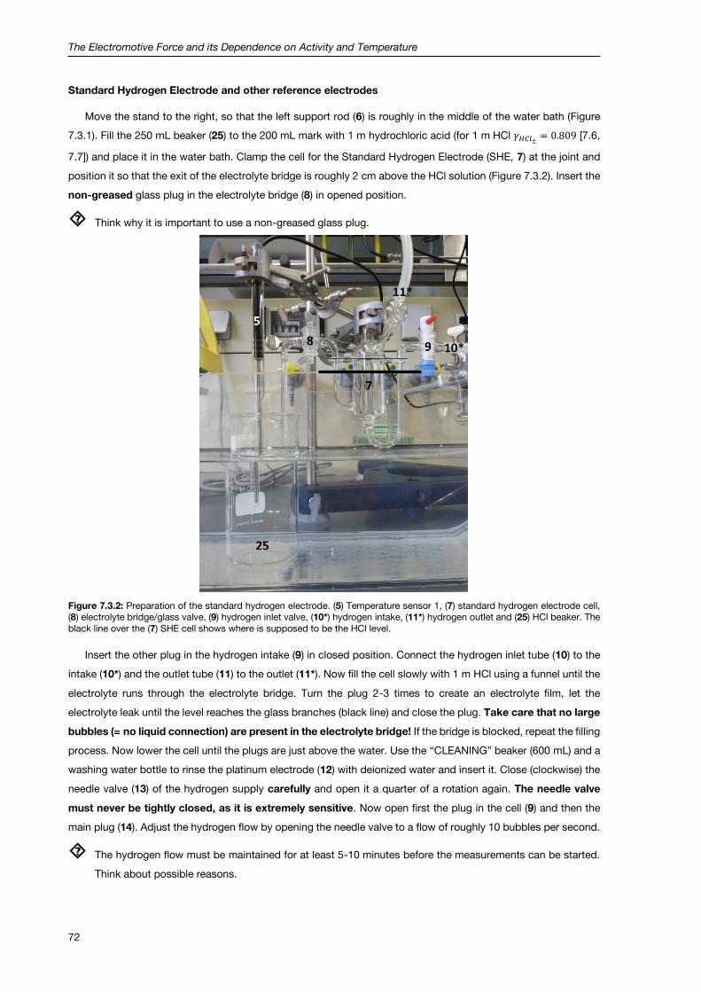
The Electromotive Force and its Dependence on Activity and Temperature
72
Standard Hydrogen Electrode and other reference electrodes
Move the stand to the right, so that the left support rod (6) is roughly in the middle of the water bath (Figure
7.3.1). Fill the 250 mL beaker (25) to the 200 mL mark with 1 m hydrochloric acid (for 1 m HCl 𝛾𝐻𝐶𝑙± = 0.809 [7.6,
7.7]) and place it in the water bath. Clamp the cell for the Standard Hydrogen Electrode (SHE, 7) at the joint and
position it so that the exit of the electrolyte bridge is roughly 2 cm above the HCl solution (Figure 7.3.2). Insert the
non-greased glass plug in the electrolyte bridge (8) in opened position.
Think why it is important to use a non-greased glass plug.
Figure 7.3.2: Preparation of the standard hydrogen electrode. (5) Temperature sensor 1, (7) standard hydrogen electrode cell, (8) electrolyte bridge/glass valve, (9) hydrogen inlet valve, (10*) hydrogen intake, (11*) hydrogen outlet and (25) HCl beaker. The black line over the (7) SHE cell shows where is supposed to be the HCl level.
Insert the other plug in the hydrogen intake (9) in closed position. Connect the hydrogen inlet tube (10) to the
intake (10*) and the outlet tube (11) to the outlet (11*). Now fill the cell slowly with 1 m HCl using a funnel until the
electrolyte runs through the electrolyte bridge. Turn the plug 2-3 times to create an electrolyte film, let the
electrolyte leak until the level reaches the glass branches (black line) and close the plug. Take care that no large
bubbles (= no liquid connection) are present in the electrolyte bridge! If the bridge is blocked, repeat the filling
process. Now lower the cell until the plugs are just above the water. Use the “CLEANING” beaker (600 mL) and a
washing water bottle to rinse the platinum electrode (12) with deionized water and insert it. Close (clockwise) the
needle valve (13) of the hydrogen supply carefully and open it a quarter of a rotation again. The needle valve
must never be tightly closed, as it is extremely sensitive. Now open first the plug in the cell (9) and then the
main plug (14). Adjust the hydrogen flow by opening the needle valve to a flow of roughly 10 bubbles per second.
The hydrogen flow must be maintained for at least 5-10 minutes before the measurements can be started.
Think about possible reasons.

The Electromotive Force and its Dependence on Activity and Temperature
73
Figure 7.3.3: Electrodes. (12) Platinum electrode, (15) calomel electrode (with a red wire inside), (16) silver-silver chloride electrode, (26) blue cap and (27) protective cap.
Screw off the blue caps (26) of the other electrodes and connect the cables. The protecting caps (27) from the
saturated calomel electrode (15, in saturated KCl, 𝛾𝐾𝐶𝑙± = 0.583 [7.7]) and the silver-silver chloride (16, Ag/AgCl,
in saturated KCl+AgCl) reference electrode are removed carefully, the electrodes are rinsed with deionized water,
wiped with paper and inserted in the HCl filled beaker (25). The temperature sensor number 1 (T1, 5) is rinsed with
deionized water, wiped with paper and inserted in the acid. All sensors and electrodes must not touch the beaker
and should be placed close to each other.
The configuration “ReferenceElectrode” is loaded on the software as described in Appendix 7.5.1. Three
separate measurements (calomel vs. SHE; Ag/AgCl vs. SHE; Ag/AgCl vs. calomel) are performed. The electrodes
are connected to the switch (17, Figure 7.3.4). The switch is connected to the Cobra4 Mobile-Link, which
measures the potential difference between working electrode (WE, red) and reference electrode (RE, blue). The
blue and black wires connect both branches of the switch to the SHE (platinum electrode). The measurements
need to be started only once the potential is steady (± 0.2 mV). Each measurement stops automatically after
3 minutes.
Figure 7.3.4: Connection of the cables and switch positions for the three reference electrode measurements: calomel electrode vs. SHE (left); Ag/AgCl vs. SHE (middle); Ag/AgCl vs. calomel electrode (right).
After all measurements are completed and the data are exported to an Excel file, the hydrogen flow is stopped
by closing first the needle valve (not completely, do not force it!), followed by the plug in the cell and the main
plug. Afterwards all electrodes are rinsed thoroughly with deionized water and stored as found. Make sure that
the white frits on the tip of the reference electrodes are in contact with the storage solution to prevent drying out.
Clean the other equipment carefully.

The Electromotive Force and its Dependence on Activity and Temperature
74
Daniell cell
After dismantling the reference electrode setup, all stand clamps must be moved high enough to move the
stand to the left (Figure 7.3.5). The stand arm (18) is lowered as much as possible. Roughly 40 mL of 0.5 m ZnSO4
(𝛾𝑍𝑛𝑆𝑂4± = 0.063) and CuSO4 solutions 0.5 m (𝛾𝐶𝑢𝑆𝑂4± = 0.062) [7.6], 0.05 m (𝛾𝐶𝑢𝑆𝑂4± = 0.201) and 0.005 m
(𝛾𝐶𝑢𝑆𝑂4± = 0.484) [7.8] are filled in the corresponding 150 mL beaker. The ZnSO4 beaker (20) is placed in the water
bath and fixed with the left clamp. The beaker with the lowest concentration of 0.005 m CuSO4 (21) is placed on
the other side.
In case that the amount of one of the zinc or copper sulfate solutions is insufficient, new solutions are prepared
from higher concentrations. To avoid contaminations, transfer 50 mL of the stock solution to the “for Preparation”
clean and labelled beakers. Since the concentrations are based on molality, thus on weight, perform weight-based
dilutions.
Rinse both temperature sensors with water, wipe them with paper and insert the first one (T1, 5) in the ZnSO4
containing beaker and the second one (T2, 5*) in the CuSO4 containing beaker. The Zn (19) and Cu (22) rods are
carefully sandpapered, rinsed with water, wiped with paper, inserted and lowered until they are dipped roughly
1 cm in their respective salt solution. Set the temperature to 25°C and wait for its rough equilibration.
Figure 7.3.5: Setup for Daniell-cell measurements. Temperature sensors (5) T1 and (5*) T2, (20) ZnSO4 beaker, (21) CuSO4 beaker and (23) electrolyte bridge.
Connect the blue cable to the Zn side of the electrode holder (24) and the red cable to the Cu side. Move the
switch in Figure 7.3.6 so that the electrodes are disconnected from the Cobra4 unit (open circuit) and connect
both cables to the switch.
Then the electrolyte bridge (23) is filled with 0.5 m NH4Cl solution using a Pasteur pipette. Make sure to
remove all air bubbles by shaking and snapping against the glass. Some electrolyte should be in the reservoir.
Rinse the black side of the salt bridge with water, wipe it before inserting one arm in each beaker. Immerse the
salt bridge only after temperature equilibration and just before starting the voltage measurement. To avoid
contaminations always make sure that the CuSO4 arm (blueish clay frit, labelled) is exclusively in contact
with CuSO4 solution and the ZnSO4 arm (white clay frit, labelled) is exclusively in contact with ZnSO4
solution.
On the software, load the configuration “DaniellElement” as described in the Appendix 7.5.1. Insert the salt
bridge, close the circuit acting on the switch and start the measurement.

The Electromotive Force and its Dependence on Activity and Temperature
75
Figure 7.3.6: Connection of the cables and switch positions for Daniell -cell measurements.
Check the electrolyte bridge, if the potential is not stable. Empty and refill it, if necessary. Stop the
measurement by clicking on the black square after you have enough data on the variability of the potential (a few
minutes should be enough) and open the circuit by acting on the switch. Transfer the data to an Excel sheet as
described in the Appendix 7.5.1.
Remove, rinse and wipe the electrolyte bridge and the second temperature sensor, move up, rinse and wipe
the Cu electrode too. Replace the CuSO4 containing beaker and repeat the measurement first for the 0.05 m and
then for the 0.5 m solution.
After investigating the variation of the thermodynamic potential with the concentration, its variation with
temperature is considered. Before this, sandpaper carefully, rinse and wipe both the electrodes again. Then use
the 1 m solutions for both the sulfates (the activity coefficients of the two solutions are very similar: 𝛾𝑍𝑛𝑆𝑂4± =
0.0435, 𝛾𝐶𝑢𝑆𝑂4± = 0.0423 [7.6]). Make sure to remove well any possible deposit formed on Zn and Cu to avoid
artifacts in the measured potential!
After dipping the electrodes in the solutions, let the temperature of both the solutions stabilise to roughly 25°C
(it takes about 10 min), leaving the electrode disconnected from the Cobra4 unit. Then connect the
measurement unit Cobra4 acting on the switch, insert the salt bridge and start to measure the potential until you
have enough collected data on its variability (five minutes should be enough). It is better to remove the salt bridge
while varying the temperature. While the two electrodes are disconnected, set the temperature of the water
bath before to 35, then to 47 °C to aim for reaction temperatures of roughly 35 and 45°C. When the temperature
is roughly reached (it takes 10–15 min), you can close the circuit acting on the switch, insert the salt bridge again
and start to measure the cell voltage again for about five minutes.
After transferring the data to Excel set the temperature back to 25 °C, clean all equipment thoroughly and
wash the electrolyte bridge once with water.
Think about an explanation why a deposit can be formed on the electrodes and why we are disconnecting
the cell while the temperature is stabilizing.
7.3.2 Data evaluation
Evaluate the reference electrode potentials comparing your measurements to the theoretical values that
you can calculate starting from the electrochemical series [7.4, 7.5], using Nernst equation and the
activity coefficients reported in the experimental execution [7.6-7.8]. Discuss deviations.
Consider the variation of the potential of the potential of the Daniell cell with the concentration of copper
sulfate. Compare your measurements to the theoretical values that you can calculate starting from the
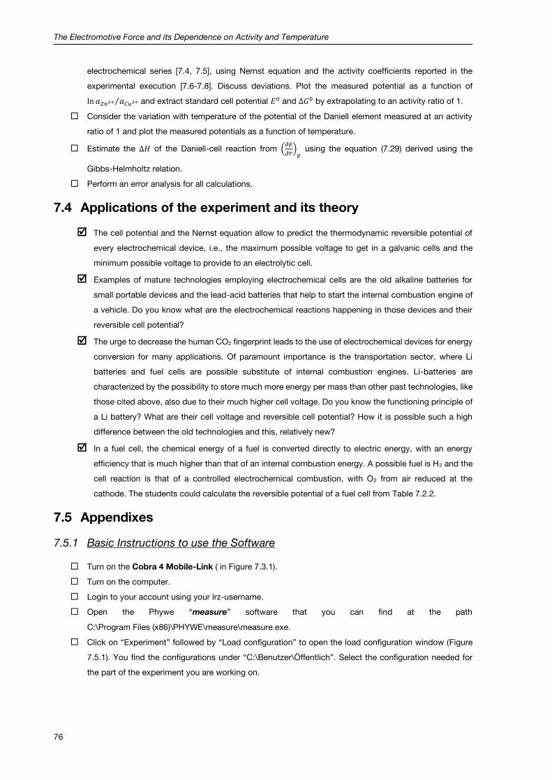
The Electromotive Force and its Dependence on Activity and Temperature
76
electrochemical series [7.4, 7.5], using Nernst equation and the activity coefficients reported in the
experimental execution [7.6-7.8]. Discuss deviations. Plot the measured potential as a function of
ln 𝑎𝑍𝑛2+ 𝑎𝐶𝑢2+⁄ and extract standard cell potential 𝐸0 and ∆𝐺0 by extrapolating to an activity ratio of 1.
Consider the variation with temperature of the potential of the Daniell element measured at an activity
ratio of 1 and plot the measured potentials as a function of temperature.
Estimate the ∆𝐻 of the Daniell-cell reaction from (𝜕𝐸
𝜕𝑇)𝑝 using the equation (7.29) derived using the
Gibbs-Helmholtz relation.
Perform an error analysis for all calculations.
7.4 Applications of the experiment and its theory
The cell potential and the Nernst equation allow to predict the thermodynamic reversible potential of
every electrochemical device, i.e., the maximum possible voltage to get in a galvanic cells and the
minimum possible voltage to provide to an electrolytic cell.
Examples of mature technologies employing electrochemical cells are the old alkaline batteries for
small portable devices and the lead-acid batteries that help to start the internal combustion engine of
a vehicle. Do you know what are the electrochemical reactions happening in those devices and their
reversible cell potential?
The urge to decrease the human CO2 fingerprint leads to the use of electrochemical devices for energy
conversion for many applications. Of paramount importance is the transportation sector, where Li
batteries and fuel cells are possible substitute of internal combustion engines. Li-batteries are
characterized by the possibility to store much more energy per mass than other past technologies, like
those cited above, also due to their much higher cell voltage. Do you know the functioning principle of
a Li battery? What are their cell voltage and reversible cell potential? How it is possible such a high
difference between the old technologies and this, relatively new?
In a fuel cell, the chemical energy of a fuel is converted directly to electric energy, with an energy
efficiency that is much higher than that of an internal combustion energy. A possible fuel is H2 and the
cell reaction is that of a controlled electrochemical combustion, with O2 from air reduced at the
cathode. The students could calculate the reversible potential of a fuel cell from Table 7.2.2.
7.5 Appendixes
7.5.1 Basic Instructions to use the Software
Turn on the Cobra 4 Mobile-Link ( in Figure 7.3.1).
Turn on the computer.
Login to your account using your lrz-username.
Open the Phywe “measure” software that you can find at the path
C:\Program Files (x86)\PHYWE\measure\measure.exe.
Click on “Experiment” followed by “Load configuration” to open the load configuration window (Figure
7.5.1). You find the configurations under “C:\Benutzer\Öffentlich”. Select the configuration needed for
the part of the experiment you are working on.

The Electromotive Force and its Dependence on Activity and Temperature
77
Figure 7.5.1: Configuration to load in the Phywe “measure” software.
To start a measurement, click on the red dot in the left upper corner (Figure 7.5.2). When the
measurement is running, a black square appears next to the position of the red dot. Clicking on it stops
the running experiment. Reference electrode measurements stop automatically after 3 minutes!
Figure 7.5.2: The upper arrow points to the red dot that has to be clicked on in order to start a measurement. The lower arrow points to the status bar, where the number of data point during the measurement is shown.
During the measurement the number of data point is shown in the status bar below the graph (Figure
7.5.2).
When the measurement is stopped, a window opens automatically and asks whether the collected data
should be saved or discarded. Transfer the collected data to the measure software (Figure 7.5.3).
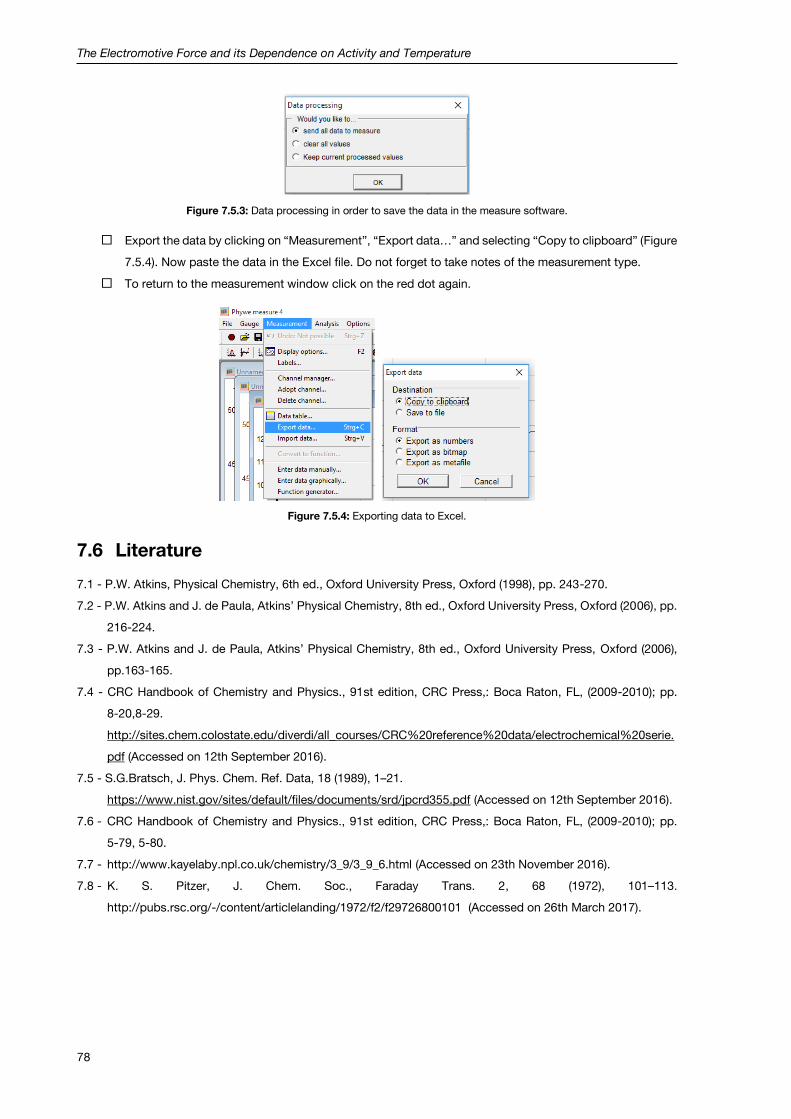
The Electromotive Force and its Dependence on Activity and Temperature
78
Figure 7.5.3: Data processing in order to save the data in the measure software.
Export the data by clicking on “Measurement”, “Export data…” and selecting “Copy to clipboard” (Figure
7.5.4). Now paste the data in the Excel file. Do not forget to take notes of the measurement type.
To return to the measurement window click on the red dot again.
Figure 7.5.4: Exporting data to Excel.
7.6 Literature
7.1 - P.W. Atkins, Physical Chemistry, 6th ed., Oxford University Press, Oxford (1998), pp. 243-270.
7.2 - P.W. Atkins and J. de Paula, Atkins’ Physical Chemistry, 8th ed., Oxford University Press, Oxford (2006), pp.
216-224.
7.3 - P.W. Atkins and J. de Paula, Atkins’ Physical Chemistry, 8th ed., Oxford University Press, Oxford (2006),
pp.163-165.
7.4 - CRC Handbook of Chemistry and Physics., 91st edition, CRC Press,: Boca Raton, FL, (2009-2010); pp.
8-20,8-29.
http://sites.chem.colostate.edu/diverdi/all_courses/CRC%20reference%20data/electrochemical%20serie.
pdf (Accessed on 12th September 2016).
7.5 - S.G.Bratsch, J. Phys. Chem. Ref. Data, 18 (1989), 1–21.
https://www.nist.gov/sites/default/files/documents/srd/jpcrd355.pdf (Accessed on 12th September 2016).
7.6 - CRC Handbook of Chemistry and Physics., 91st edition, CRC Press,: Boca Raton, FL, (2009-2010); pp.
5-79, 5-80.
7.7 - http://www.kayelaby.npl.co.uk/chemistry/3_9/3_9_6.html (Accessed on 23th November 2016).
7.8 - K. S. Pitzer, J. Chem. Soc., Faraday Trans. 2, 68 (1972), 101–113.
http://pubs.rsc.org/-/content/articlelanding/1972/f2/f29726800101 (Accessed on 26th March 2017).

79
8 Activation Energy of a First-Order Reaction
8.1 Context and aim of the experiment
In this experiment, the activation energy of a first-order reaction is estimated. To do this, the activation energy
is determined by measuring the temperature dependence of a reaction rate constant [8.1 - 8.5].
8.1.1 Important concepts to know
Reaction kinetics, reaction rate constant, rate-limiting step, reaction order, Arrhenius equation, activation
energy, integration of the differential equation for first-order reactions, conductivity, reaction coordinate, half-life,
elementary reactions, molecularity.
8.1.2 Most common questions to be answered
How can you prove graphically the existence of a first-order reaction?
Can the activation energy change with temperature? If yes, think about an explanation.
What indicates a non-linear Arrhenius behavior?
Think about the pre-exponential factor of the Arrhenius equation. How does it change for different types of
reactions?
What is the unit of the measured conductivity? Try to explain it in a more familiar way. How you can derive
the unit for the conductivity from the setting of the used electrode?
8.1.3 Further preparations before the experiment
Before performing the experiment, prepare a worksheet as follows:
Table 8.1.1: Example of the table to prepare for data collection and evaluation.
𝑇 = … K
t (s) 𝜒𝐶
(S cm-1) 𝜒𝐶𝐸 − 𝜒𝐶 (S cm-1)
𝜒𝐶𝐸𝜒𝐶𝐸 − 𝜒𝐶
… … … …
… … … …
… … … …
… … … …
8.2 Theory
In biology and chemistry, the analysis of reaction kinetics has two important impacts. On one hand, it is
possible to investigate reaction mechanisms and on the other hand, it is very interesting to know the rates, which
are quite high for many reactions of interest.
8.2.1 Reaction rate, reaction order and molecularity
For a reaction with 𝑖 partners, the reaction rate 𝑣 is defined as
𝑣 =1
𝜈𝑖
𝑑[𝑖]
𝑑𝑡 (8.1)
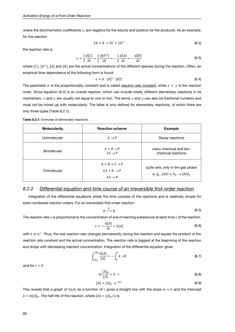
Activation Energy of a First-Order Reaction
80
where the stoichiometric coefficients 𝜈𝑖 are negative for the educts and positive for the products. As an example,
for the reaction
2𝐴 + 𝐵 → 3𝐶 + 2𝐻+ (8.2)
the reaction rate is
𝑣 =1
3
𝑑[𝐶]
𝑑𝑡=1
2
𝑑[𝐻+]
𝑑𝑡= −
1
2
𝑑[𝐴]
𝑑𝑡= −
𝑑[𝐵]
𝑑𝑡 (8.3)
where [𝐶], [𝐻+], [𝐴] and [𝐵] are the actual concentrations of the different species during the reaction. Often, an
empirical time dependence of the following form is found
𝑣 = 𝑘 ∙ [𝐴]𝑥 ∙ [𝐵]𝑦 (8.4)
The parameter 𝑘 is the proportionality constant and is called reaction rate constant, while 𝑥 + 𝑦 is the reaction
order. Since equation (8.2) is an overall reaction, which can include totally different elementary reactions in its
mechanism, 𝑥 and 𝑦 are usually not equal to one or two. The terms 𝑥 and 𝑦 can also be fractional numbers and
must not be mixed up with molecularity. The latter is only defined for elementary reactions, of which there are
only three types (Table 8.2.1).
Table 8.2.1: Overview of elementary reactions.
Molecularity Reaction scheme Example
Unimolecular 𝐴 𝑃 Decay reactions
Bimolecular 𝐴 + 𝐵 𝑃 2𝐴 𝑃
many chemical and bio- chemical reactions
Trimolecular
𝐴 + 𝐵 + 𝐶 𝑃
2𝐴 + 𝐵 𝑃
3𝐴 𝑃
quite rare, only in the gas phase
e. g., 2𝑁𝑂 + 𝑂2 2𝑁𝑂2
8.2.2 Differential equation and time course of an irreversible first-order reaction
Integration of the differential equations yields the time courses of the reactions and is relatively simple for
even-numbered reaction orders. For an irreversible first-order reaction:
𝐴 𝑘 → 𝐵 (8.5)
The reaction rate 𝑣 is proportional to the concentration of one of reacting substances at each time 𝑡 of the reaction.
𝑣 = −𝑑[𝐴]
𝑑𝑡= 𝑘[𝐴] (8.6)
with 𝑘 in s-1. Thus, the real reaction rate changes permanently during the reaction and equals the product of the
reaction rate constant and the actual concentration. The reaction rate is biggest at the beginning of the reaction
and drops with decreasing reactant concentration. Integration of the differential equation gives
∫𝑑[𝐴]
[𝐴]
[𝐴]𝑡
[𝐴]0
= −∫ 𝑘 ∙ 𝑑𝑡𝑡
0
(8.7)
and for 𝑡 = 0
ln[𝐴]0[𝐴]
= 𝑘 ∙ 𝑡 (8.8)
[𝐴] = [𝐴]0 ∙ 𝑒−𝑘∙𝑡 (8.9)
This reveals that a graph of ln[𝐴] as a function of 𝑡 gives a straight line with the slope 𝑚 = 𝑘 and the intercept
𝑏 = ln[𝐴]0. The half-life of the reaction, where [𝐴] = [𝐴]0 2⁄ is

Activation Energy of a First-Order Reaction
81
𝑡1/2 =1
𝑘∙ ln 2 (8.10)
8.2.3 Temperature dependence of a reaction rate constant
Van’t Hoff and Arrhenius empirically found that the temperature dependence of reaction rate constants often
could be described using the following equation
𝑘 = 𝐴 ∙ 𝑒−𝐸𝐴𝑅∙𝑇 (8.11)
This relation is called Arrhenius equation. 𝐴 is the Arrhenius pre-exponential factor, that is the rate constant in
case all the collisions lead to reaction. Additionally, 𝐴 includes a steric factor, which takes into account that the
reactants have to be properly aligned during the collision for the reaction to occur. 𝐸𝐴 is the Arrhenius activation
energy, which can vary a lot comparing different reactions. In the Arrhenius equation we can see a Boltzmann
factor, which gives the fraction of molecules with energy higher than 𝐸𝐴 (see Figure 8.2.1) and a constant,
temperature-independent pre-exponential factor 𝐴. According to the Maxwell-Boltzmann equation, the number
of molecules with kinetic energy higher than 𝐸𝐴 is dependent on temperature.
Figure 8.2.1: Molecular interpretation of the activation energy.
Equation (8.11) is only valid in a relatively small temperature region, therefore it is better to write
𝑑(ln 𝑘)
𝑑𝑇=
𝐸𝐴𝑅 ∙ 𝑇2
(8.12)
or
𝑑(ln 𝑘)
𝑑(1 𝑇⁄ )= −
𝐸𝐴𝑅
(8.13)
and
ln𝑘1𝑘2
=𝐸𝐴𝑅(1
𝑇2−1
𝑇1) (8.14)
Thus, the activation energy can be determined graphically by plotting ln 𝑘 versus 1/𝑇. This plot is called Arrhenius
plot (see Figure 8.2.2).
Figure 8.2.2: Schematic depiction of an Arrhenius plot.

Activation Energy of a First-Order Reaction
82
8.2.4 Correlation between activation energy and reaction enthalpy
For the reversible reaction
𝐴
𝑘𝑓𝑜𝑟𝑤→
𝑘𝑏𝑎𝑐𝑘←
𝐵 (8.15)
with the equilibrium constant
𝐾 =𝑘𝑓𝑜𝑟𝑤
𝑘𝑏𝑎𝑐𝑘 (8.16)
we obtain
𝑑(ln 𝑘𝑓𝑜𝑟𝑤)
𝑑𝑇−𝑑(ln 𝑘𝑏𝑎𝑐𝑘)
𝑑𝑇=𝑑(ln𝐾)
𝑑𝑇=
∆𝐻0
𝑅 ∙ 𝑇2 (8.17)
where ∆𝐻0 is the Van’t Hoff enthalpy or reaction enthalpy. This shows that the activation energy is directly
correlated to the reaction enthalpy (see Figure 8.2.3).
𝐸𝐴,𝑏𝑎𝑐𝑘 − 𝐸𝐴,𝑓𝑜𝑟𝑤 = Δ𝐻0 (8.18)
Figure 8.2.3: Correlation between the activation energy and the reaction enthalpy.
8.2.5 Decomposition of the tertiary amylbromide
In this experiment, the decay of tertiary amylbromide is considered
𝐶2𝐻5(𝐶𝐻3)2𝐶𝐵𝑟 ⟶ [𝐶2𝐻5(𝐶𝐻3)2𝐶+] + 𝐵𝑟− slow (8.19)
[𝐶2𝐻5(𝐶𝐻3)2𝐶+] + 𝐻2𝑂 → 𝐶2𝐻5(𝐶𝐻3)2𝐶𝑂𝐻 + 𝐻+ fast (8.20)
Following a SN1 reaction mechanism, tertiary amylbromide decomposes in solution into bromide ions and a
tertiary amyl cation. The latter reacts instantaneously with water, forming a non-dissociated alcohol. The
rate-determining step for the overall reaction is the decomposition of amylbromide, which is a first-order reaction.
If 𝑥 designates the reaction turnover (concentration of HBr produced) then the concentration 𝑐 of amylbromide
is
𝑐 = 𝑐0 − 𝑥 (8.21)
HBr is present in its dissociated form. Therefore, its concentration can be followed by conductivity measurements.
The turnover is proportional to the conductivity 𝜒𝐶 in the measuring cell. The final conductivity 𝜒𝐶𝐸, reached when
the reaction process is completed, is proportional to the initial concentration 𝑐0 of amylbromide. Thus, measuring
the conductivity provides an easy way to follow the change in concentration during the reaction process.
The above approach yields
𝑐0𝑐=
𝑐0𝑐0 − 𝑥
=𝜒𝐶𝐸
𝜒𝐶𝐸 − 𝜒𝐶 (8.22)
and equation (8.8) can be converted to

Activation Energy of a First-Order Reaction
83
ln𝜒𝐶𝐸
𝜒𝐶𝐸 − 𝜒𝐶= 𝑘 ∙ 𝑡 (8.23)
8.3 Experimental details and evaluation
8.3.1 Experimental execution
The conductivity measurements are performed with special conductivity electrodes (3) (see Figure 7.3.2) that
provide simultaneously the temperature of the solution.
Figure 8.3.1: Experimental setup in all its parts. (1) Cobra 4 Mobile-Link, (2) measuring cell, (3) conductivity electrode, (4) magnetic stirrer, (5) thermostat, (5*) buttons to regulate the set temperature, (6) valve to turn on and off the cooling water, (7) tubes connecting measuring cell and thermostat.
Turn on the equipment for conductivity measurement: the Cobra 4 Mobile-Link (1) and the computer (for basic
instructions how to use the software, see the Appendix 8.5.1). Clean the measuring cell (2) thoroughly. Always
be careful to handle delicate equipment. First, rinse the conductivity electrode (3) with ethanol. Then take the
glass cell (2) from the holder and rinse it once with alcohol over a washbowl. For washing use the ethanol provided
in the plastic bottle, not the concentrated 80 vol% ethanol in the glass bottle. Furthermore, clean the stirring bar
with alcohol and put it into the measuring cell (2).
Now, fill the cell with 80 mL of 80 vol% ethanol from the glass bottle and insert the electrode. The probe has
to be immersed completely in the solvent. Then, turn on the thermostat (5) and adjust the temperature in order to
obtain 𝑇 = 25 0.5 C in the reaction solution. The set temperature of the thermostat can be adjusted by pressing
the yellow button (5*) of the thermostat twice. The display starts blinking and the set temperature can be regulated
using the red and blue buttons with the arrows pointing up and down (5*). Finally, the yellow button (5*) has to be
pressed once in order to confirm the set temperature. Do not forget to turn on the cooling water! (6). Also turn
on the magnetic stirrer (4), but take care that it does not touch the conductivity probe.
When the solvent has reached the desired temperature, add 0.5 mL of tertiary amylbromide trough one of the
openings in the measuring cell, using a clean and dry pipette. It is important that the amount of amylbromide
is measured exactly.
Measure the conductivity as a function of time at 𝑇 = 25(0.5) C and then clean cell and electrode and repeat
the same experiment at 𝑇 = 30(0.5) C and 𝑇 = 35(0.5) C as a function of time for each temperature. At
𝑇 = 25 C and 𝑇 = 30 C data collection has to last 30 minutes. At 𝑇 = 35 C the conductivity measurement has
to last until the reaction process is finished.

Activation Energy of a First-Order Reaction
84
Think about how you can ensure that the reaction process is finished and discuss it with your supervisor
before you start the experiment.
As mentioned above, it is important that the amount of amylbromide is measured exactly. What happens if
the initial concentration of amylbromide varies for the three measurements?
Enter the collected data in the prepared table (see Table 8.1.1). At 𝑇 = 25 C and 𝑇 = 30 C, the final
conductivity 𝜒𝐶𝐸 is reached only after quite a long time. Therefore, 𝜒𝐶𝐸 for all temperatures is measured using the
solution of the measurement at 𝑇 = 35 C where the reaction has completed. To do this, set the thermostat (5) to
20 C and add ice into the water reservoir of the thermostat to speed up the cooling process. Take care that the
water does not overflow.
How can you explain that the final conductivity varies for different temperatures?
8.3.2 Data evaluation
Plot 𝑙𝑛(𝜒𝐶𝐸 𝜒𝐶𝐸 − 𝜒𝐶⁄ ) as a function of time for the three temperatures and determine the reaction-rate
constant 𝑘 from the slope of the straight line according to equation (8.23). Use an adequate number of
data points for this evaluation.
Determine the half-life 𝑡1/2 of the reaction for the three temperatures.
Plot 𝑙𝑛 𝑘 vs. 1/𝑇 and determine the activation energy 𝐸𝐴 from the resulting straight line.
Perform an error analysis for all calculations.
8.4 Applications of the experiment and its theory
The effect of temperature on reaction rate constants is important in everyday life, e.g. for increasing
the storage life of food by keeping it in your fridge.
Activation energy for combustion reactions. E.g., in the petrol engine, the activation energy for the
combustion of the present mixture of air and gaseous petrol is provided by an electrical ignition spark
(heat energy). By comparison, in the diesel engine the activation energy for starting the combustion of
diesel is based only on compression of the mixture of air and diesel fuel.
Lighting a match: frictional heat and pressure provide the activation energy for spontaneous ignition of
chlorate and red phosphor.
Frictional heat provides the activation energy for the explosion of cap bombs.
Characterization of the free energy barrier for chemical and biochemical reactions. Comparison to the
general rate equation allows determination of enthalpic contributions (activation enthalpy) and entropic
contributions (activation entropy) to the energy barrier.
Investigation of the kinetic activity of catalysts.
8.5 Appendixes
8.5.1 Basic Instructions to use the Software
Turn on the Cobra 4 Mobile-Link (1) in Figure 8.3.1.
Turn on the computer.
Login to your account using your lrz-username.

Activation Energy of a First-Order Reaction
85
Open the Phywe “measure” software that you can find at the path
C:\Program Files (x86)\PHYWE\measure\measure.exe.
Click on “Experiment” followed by “Load configuration” to open the load configuration window (Figure
8.5.1). You find the configurations under “C:\Benutzer\Öffentlich”. Select the configuration needed for
the experiment you are working on.
Figure 8.5.1: Configuration to load in the Phywe “measure” software.
The measurement has to be started before the amylbromide is added. This allows determination of the
basic value for the conductivity. The time point of amylbromide addition reflects the zero time point (𝑡 =
0) for the experiment.
To start a measurement, click on the red dot in the left upper corner (Figure 8.5.2).
Figure 8.5.2: The arrow points to the red dot that has to be clicked on in order to start a conductivity measurement. When the measurement is running, a black square appears at the position of the red dot. Clicking on it does stop the running experiment.
The data collected during a measurement are shown in a table in the navigator (Figure 8.5.3).
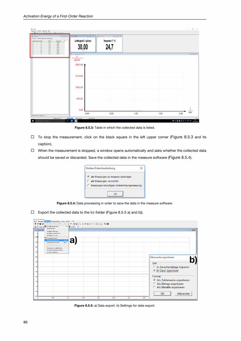
Activation Energy of a First-Order Reaction
86
Figure 8.5.3: Table in which the collected data is listed.
To stop the measurement, click on the black square in the left upper corner (Figure 8.5.3 and its
caption).
When the measurement is stopped, a window opens automatically and asks whether the collected data
should be saved or discarded. Save the collected data in the measure software (Figure 8.5.4).
Figure 8.5.4: Data processing in order to save the data in the measure software.
Export the collected data to the lrz-folder (Figure 8.5.5 a) and b)).
Figure 8.5.5: a) Data export. b) Settings for data export.
a)
b)

Activation Energy of a First-Order Reaction
87
8.6 Literature
8.1 - P.W. Atkins, Physical Chemistry, 6th ed., Oxford University Press, Oxford (1998), pp. 761-777.
8.2 - P.W. Atkins and J. de Paula, Atkins’ Physical Chemistry, 8th ed., Oxford University Press, Oxford (2006),
pp. 791-808.
8.3 - G. Wedler, Lehrbuch der Physikalischen Chemie, 6th ed., Wiley/VCH (2012).
8.4 - W.J. Moore, Grundlagen der Physikalischen Chemie, 1st ed., de Gruyter (1990).
8.5 - R. Brdicka, Grundlagen der Physikalischen Chemie, 15th ed., Willey/VCH (1981).

88
9 Kinetics of the Inversion of Sucrose
9.1 Context and aim of the experiment
The inversion of sucrose is a reaction that can be catalyzed in acidic environment. In this experiment,
polarimetric measurements are performed in order to investigate the reaction rate at different acid concentrations.
The obtained data are used to define the reaction-rate constant [9.1 - 9.3].
9.1.1 Important concepts to know
Kinetics, reaction-rate constant, rate-determining step, thermodynamics, equilibrium constant, catalyst,
activation energy, reaction enthalpy, reaction order, molecularity, integration of the differential equation for first-
order reactions, reaction coordinates, polarimetry, polarization of light, optically-active molecules, Law of Biot,
Law of Malus.
9.1.2 Most common questions to be answered
How can you prove graphically the existence of a first-order reaction or a pseudo-first-order reaction?
What are the requirements for a pseudo-first-order reaction?
How can polarized light be produced?
What is an optically active substance? Give some examples.
How does a catalyst act on the kinetics and on the thermodynamics of a reaction?
9.1.3 Further preparations before the experiment
Before performing the experiment, prepare a worksheet as follows:
Table 9.1.1: Example of the table to prepare for data collection and evaluation. 𝛼𝑒𝑥𝑝 stands for the individual rotation angles that are determined experimentally.
sample
𝑡 (s) 𝛼𝑒𝑥𝑝 (°) 1
𝑛∑ 𝛼𝑒𝑥𝑝,𝑖𝑛𝑖=1 (°) ln
𝛼(𝑡) − 𝛼∞𝛼0 − 𝛼∞
… … … …
… … … …
… … … …
… … … …
9.2 Theory
9.2.1 Catalytic reactions
The function of a catalysts can be explained as its effect on decreasing the activation energy 𝐸𝐴 of a reaction.
This decrease can affect dramatically the reaction-rate constant 𝑘 of a reaction, since 𝐸𝐴 is at the exponent of the
Arrhenius equation (see equation (8.11) in Chapter 8) [9.4]. During catalysis, the reactants and the catalyst are
forming one or more intermediate states 𝑧 and the highest activation energy of this new mechanism is smaller
than the activation energy of the reaction without catalyst (Figure 9.2.1); for this reason, the reaction proceeds
faster. The catalyst itself is not used up, but it is regenerated after product formation, like in a cycle. A single

Kinetics of the Inversion of Sucrose
89
catalyst can thus run through several catalytic cycles. Since the forward and the backward reaction are
accelerated equally, the catalyst does change the kinetics of the reaction but not its thermodynamics (enthalpy
∆𝐻0).
Figure 9.2.1: A catalyst provides a different reaction path with a lower activation energy. The energy profile of the reaction is shown in absence (black line) and in presence (red line) of a catalyst.
In catalysis, the most important reaction mechanism is a series of sequential reactions in which the first step
is bimolecular:
𝐶𝑎𝑡 + 𝑆
𝑘12 →
𝑘21 ←
𝐶𝑎𝑡𝑆 𝑘23 → 𝐶𝑎𝑡𝑃 ⟶ 𝐶𝑎𝑡 + 𝑃 (9.1)
where 𝐶𝑎𝑡 stands for the catalyst, 𝑆 for the substrate (the reactant which is bound to the catalyst) and 𝑃 for the
product. The general mathematical solution for this mechanism is complex, but it can be simplified if certain
assumptions are fulfilled.
9.2.2 Kinetics of first-order and pseudo-first-order reactions
Catalytic reaction mechanisms always contain bimolecular steps (Equation (9.1)) but the analysis of a
second-order kinetics is complex. The reaction rate 𝑣 for an irreversible, heterogeneous, second-order reaction
of the type
𝐶𝑎𝑡 + 𝑆 𝑘𝑏𝑖𝑚𝑜𝑙 → 𝐶𝑎𝑡𝑆 (9.2)
is
𝑣 = −𝑑[𝐶𝑎𝑡]
𝑑𝑡= −
𝑑[𝑆]
𝑑𝑡= 𝑘𝑏𝑖𝑚𝑜𝑙 ∙ [𝐶𝑎𝑡] ∙ [𝑆] (9.3)
Equation (9.3) can be simplified if one of the involved species is in large excess (at least fivefold excess). For
instance, if 𝐶𝑎𝑡 is present in large excess, its concentration can be approximated to be constant throughout the
reaction. Thus, [𝐶𝑎𝑡] can be approximated by [𝐶𝑎𝑡]0 and the rate law becomes apparent first-order. The reaction
rate 𝑣 is then proportional to the concentration of the reactant present at low concentration at each time point of
the reaction.
𝑣 = −𝑑[𝑆]
𝑑𝑡= 𝑘′ ∙ [𝑆] with 𝑘′ = 𝑘𝑏𝑖𝑚𝑜𝑙 ∙ [𝐶𝑎𝑡] (9.4)
Reactions in which the observed kinetics is first-order but the mechanism is second-order are referred to as
pseudo-first-order reactions. The integration of the differential equation
∫𝑑[𝑆]
[𝑆]
[𝑆]𝑡
[𝑆]0
= ∫ 𝑘′ ∙ 𝑑𝑡𝑡
0
(9.5)
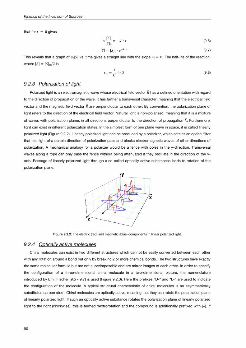
Kinetics of the Inversion of Sucrose
90
that for 𝑡 = 0 gives
ln[𝑆]
[𝑆]0= −𝑘′ ∙ 𝑡 (9.6)
[𝑆] = [𝑆]0 ∙ 𝑒−𝑘′∙𝑡 (9.7)
This reveals that a graph of ln[𝑆] vs. time gives a straight line with the slope 𝑚 = 𝑘’. The half-life of the reaction,
where [𝑆] = [𝑆]0/2 is
𝑡½ =1
𝑘′∙ ln 2 (9.8)
9.2.3 Polarization of light
Polarized light is an electromagnetic wave whose electrical field vector �⃑� has a defined orientation with regard
to the direction of propagation of the wave. It has further a transversal character, meaning that the electrical field
vector and the magnetic field vector �⃑� are perpendicular to each other. By convention, the polarization plane of
light refers to the direction of the electrical field vector. Natural light is non-polarized, meaning that it is a mixture
of waves with polarization planes in all directions perpendicular to the direction of propagation �⃑� . Furthermore,
light can exist in different polarization states. In the simplest form of one plane wave in space, it is called linearly
polarized light (Figure 9.2.2). Linearly polarized light can be produced by a polarizer, which acts as an optical filter
that lets light of a certain direction of polarization pass and blocks electromagnetic waves of other directions of
polarization. A mechanical analogy for a polarizer would be a fence with poles in the y-direction. Transversal
waves along a rope can only pass the fence without being attenuated if they oscillate in the direction of the y-
axis. Passage of linearly polarized light through a so-called optically active substances leads to rotation of the
polarization plane.
Figure 9.2.2: The electric (red) and magnetic (blue) components in linear polarized light.
9.2.4 Optically active molecules
Chiral molecules can exist in two different structures which cannot be easily converted between each other
with any rotation around a bond but only by breaking 2 or more chemical bonds. The two structures have exactly
the same molecular formula but are not superimposable and are mirror images of each other. In order to specify
the configuration of a three-dimensional chiral molecule in a two-dimensional picture, the nomenclature
introduced by Emil Fischer [9.5 - 9.7] is used (Figure 9.2.3). Here the prefixes “D-“ and “L-“ are used to indicate
the configuration of the molecule. A typical structural characteristic of chiral molecules is an asymmetrically
substituted carbon atom. Chiral molecules are optically active, meaning that they can rotate the polarization plane
of linearly polarized light. If such an optically active substance rotates the polarization plane of linearly polarized
light to the right (clockwise), this is termed dextrorotation and the compound is additionally prefixed with (+). If

Kinetics of the Inversion of Sucrose
91
the polarization plane is rotated to the left (counter clockwise), this is termed levorotation and the compound is
additionally prefixed with (-).
Figure 9.2.3: Fisher projection of D-glucose (left) and L-glucose (right).
9.2.5 Polarimetry
The rotatory dispersion resulting from linearly polarized light passing through an optically active substance
provides the basis for polarimetric measurements. The typical setup for a polarimetric experiment is sketched in
Figure 9.2.4. It consists of a light source (often a sodium-vapor discharge lamp) that produces non-polarized light,
a polarizer (Nicol-prism), a measuring cell filled with the sample and a second polarizer (called analyzer, rotatable
Nicol-prism) that probes the polarization state after passage of the light through the sample.
Figure 9.2.4: Sketch of the typical setup for a polarimetric experiment.
The angle 𝛼 of rotation is given by
𝛼 = [𝛼]𝜆𝑇 ⋅ 𝑐 ⋅ 𝑙 (9.9)
where 𝑐 denotes the concentration of the optically active substance in g/mL. The parameter 𝑙 is the length of the
measuring cell in dm. [𝛼]𝜆𝑇 is the specific rotation of a substance at a certain wavelength 𝜆 and temperature 𝑇 and
it corresponds to the rotation angle detected for 1 g of the optically active substance in 1 mL solution along a
path length 𝑙 = 1 dm. In order to use the concentration in mol/L, being 𝑀 the molar mass of the optically-active
substance, the following relationship needs to be used
𝑐 [𝑔
𝑚𝐿] =
1
1000∙ 𝑀[
𝑔
𝑚𝑜𝑙] ∙ 𝑐[
𝑚𝑜𝑙
𝐿] (9.10)
The Malus’ law describes the intensity 𝐼 of the passed light as a function of the initial light intensity 𝐼0 and the
angle 𝛼 as
𝐼 = 𝐼0 ∙ 𝑐𝑜𝑠2(𝛼) (9.11)
9.2.6 Optical activity and decomposition of sucrose
Sucrose (also called saccharose) is the common crystalline sugar used in household. It is a disaccharide
consisting of glucose and fructose. In acidic aqueous solution, sucrose is thermodynamically instable and

Kinetics of the Inversion of Sucrose
92
decomposes hydrolytically in -D-Glucose and -D-Fructose (Figure 9.2.5). The resulting mixture of glucose and
fructose with equal amount of substance is called invert sugar. Equilibrium is reached which lies almost completely
on the right side of the reaction, thus the reaction can be viewed as irreversible. In the absence of an acid, almost
no sucrose is cleaved.
(sucrose) -D-Glucose -D-Fructose
Figure 9.2.5: Hydrolytic decomposition of sucrose in acidic solution.
The overall reaction process (as shown in Figure 9.2.5) consists of different sub-reactions (Figure 9.2.6).
Figure 9.2.6: Role of H+ during cleavage of sucrose. Note that protons are not consumed but released at the end of the process, thus acting as catalysts for the hydrolytic decomposition.
Addition of an acid leads to protonation of the oxygen atom that bonds glucose and fructose in the disaccharide.
The equilibrium of the protonation reaction is reached very fast. Thereby, the positive partial charge of the
neighboring carbon atoms is increased, allowing the attack of the free electron pairs of the oxygen atom in water
at this site. This leads to cleavage of the disaccharide and to subsequent deprotonation. Since protons are not
consumed but released at the end of the process, they act as catalysts.
Formally, inversion of sucrose is thus a third-order reaction. Note that the reaction order can only be determined
experimentally. For the inversion of sucrose results reveal a first-order reaction. This can be explained by the fact
that a trimolecular elementary reaction is extremely unlikely (see Table 8.2.1), since in this case three molecules
have to collide simultaneously. Such reactions usually occur in two consecutive bimolecular steps, as it is also
the case for the inversion of sucrose (see Figure 9.2.6). Take care that you are familiar with the term of elementary
reaction, molecularity and reaction order and for this see paragraph 8.2.1.
In the case of the inversion of sucrose, the second bimolecular step is significantly slower compared to the first
one (𝑘12 ≫ 𝑘23) and thus represents the rate-limiting step. Therefore, the protonation step is described as a fast
pre-equilibrium, which depends on the degree of dissociation of the available acid.
𝑆(𝑎𝑞) + 𝐻+(𝑎𝑞)
𝑘12 →
𝑘21 ←
𝑆𝐻+(𝑎𝑞) 𝑘23 → 𝐺(𝑎𝑞) + 𝐹(𝑎𝑞) + 𝐻+(𝑎𝑞) (9.12)
Here 𝑆, 𝐺 and 𝐹 denote sucrose, glucose and fructose, respectively. Note that this mechanism is in agreement
with the mechanism usually found for catalyzed reactions (Equation (9.2)). For the kinetics of the decomposition
of sucrose and for the formation of product we can write:

Kinetics of the Inversion of Sucrose
93
−𝑑[𝑆]
𝑑𝑡=𝑑[𝐺]
𝑑𝑡=𝑑[𝐹]
𝑑𝑡= 𝑘23 ∙ [𝑆𝐻
+] ∙ [𝐻2𝑂] (9.13)
The concentration [𝑆𝐻+] of protonated sucrose is determined by the pre-equilibrium:
𝑆 + 𝐻+
𝑘12 →
𝑘21 ←
𝑆𝐻+ (9.14)
and it is thus given by
[𝑆𝐻+] = 𝐾 ⋅ [𝑆] ⋅ [𝐻+] (9.15)
where
𝐾 =𝑘12𝑘21
=[𝑆𝐻+]
[𝑆] ⋅ [𝐻+] (9.16)
According to Equation (9.15), Equation (9.13) becomes
−𝑑[𝑆]
𝑑𝑡= 𝑘23 ∙ 𝐾 ⋅ [𝑆] ⋅ [𝐻+] ∙ [𝐻2𝑂] (9.17)
Considering that the concentration of protons stays constant allows inclusion of [𝐻+] into the effective reaction-
rate constant
𝑘′ = 𝑘23 ⋅ 𝐾 ⋅ [𝐻+] (9.18)
This leads to
−𝑑[𝑆]
𝑑𝑡= 𝑘′ ⋅ [𝑆] ∙ [𝐻2𝑂] (9.19)
The amount of water does hardly change during the reaction since it is present in large excess (pseudo-first-order
conditions) and thus, [𝐻2𝑂] can also be added to the rate constant and one obtains the pseudo-first-order rate
constant 𝑘’’
𝑘′′ = 𝑘′ ∙ [𝐻2𝑂] (9.20)
This explains the experimentally observed first-order reaction. A second-order reaction that can be approximated
to a first-order reaction since one of the reactants is present in large excess is called a pseudo-first order reaction
(see paragraph 9.2.2). The decomposition of sucrose can now be written as
−𝑑[𝑆]
𝑑𝑡= 𝑘′′ ⋅ [𝑆] (9.21)
By solving the differential equation for the concentration of sucrose as in Equation (9.5), we can obtain the relation
with time of the decomposition of sucrose as in Equations (9.6) and (9.7)
All three sugars that are involved in the reaction under investigation are optically active due to their
asymmetrical carbon atom (Table 9.2.1). This allows determination of the reaction rate from polarimetric
measurements.
Table 9.2.1: Specific rotations 𝛼 at T = 20 C and = 598.3 nm for the species involved in the inversion of sucrose. Data taken from [2.9].
Substance 𝛼 (°)
Sucrose +66.5
D-Glucose +52.7
D-Fructose -92.4
1/1 mol/molD-Glucose/D-Fructose -19.8
Based on Equation (9.9) and using the concentration given in mol/L, the rotation angle 𝛼0 at the beginning of
the reaction is
𝛼0 = 𝑙 ⋅ 1000 ⋅ 𝑀𝑆 ⋅ 𝛼𝜆,𝑆𝑇 ⋅ [𝑆]0 (9.22)

Kinetics of the Inversion of Sucrose
94
where 𝑀𝑆 is the molecular weight of the sucrose.
At any point of the reaction the actual total rotation angle 𝛼(𝑡) corresponds to the sum of the contributions of the
existing species.
𝛼(𝑡) = 𝛼𝑆 + 𝛼𝐺 + 𝛼𝐹 =
= 𝑙 ⋅ 1000 ⋅ {𝑀𝑆 ⋅ 𝛼𝜆,𝑆𝑇 ⋅ [𝑆] + 𝑀𝐺 ⋅ 𝛼𝜆,𝐺
𝑇 ⋅ [𝐺] + 𝑀𝐹 ⋅ 𝛼𝜆,𝐹𝑇 ⋅ [𝐹]}
(9.23)
Considering that [𝐺] = [𝐹] = [𝑆]0 − [𝑆] (from Equation (9.12)) we can write:
𝛼(𝑡) =
= 𝑙 ⋅ 1000 ⋅ {𝑀𝑆 ⋅ 𝛼𝜆,𝑆𝑇 ⋅ [𝑆] + 𝑀𝐺 ⋅ 𝛼𝜆,𝐺
𝑇 ⋅ [𝐺] + 𝑀𝐹 ⋅ 𝛼𝜆,𝐹𝑇 ⋅ [𝐹]}=
= 𝑙 ⋅ 1000 ⋅ {𝑀𝑆 ⋅ 𝛼𝜆,𝑆𝑇 ⋅ [𝑆] + (𝑀𝐺 ⋅ 𝛼𝜆,𝐺
𝑇 +𝑀𝐹 ⋅ 𝛼𝜆,𝐹𝑇 ) ⋅ ([𝑆]0 − [𝑆])} =
= 𝑙 ⋅ 1000 ⋅ {(𝑀𝐺 ⋅ 𝛼𝜆,𝐺𝑇 +𝑀𝐹 ⋅ 𝛼𝜆,𝐹
𝑇 ) ⋅ [𝑆]0 + (𝑀𝑆 ⋅ 𝛼𝜆,𝑆𝑇 −𝑀𝐺 ⋅ 𝛼𝜆,𝐺
𝑇 −𝑀𝐹 ⋅ 𝛼𝜆,𝐹𝑇 ) ⋅ [𝑆]}
(9.24)
The reactant sucrose turns the polarization plane of linearly polarized light to the right while the equimolar mixture
of glucose and fructose that is formed during the inversion reaction, turns it to the left (Table 9.2.1). As a result,
the polarization plane of linearly polarized light turns more and more to the left and the overall rotation angle
becomes smaller and smaller as the inversion reaction proceeds. At the end, the overall rotation angle becomes
even negative. This is the reason for the name of the produced inverted sugar. When the reaction is completed,
the final rotation angle 𝛼∞ (with 𝑡 → ∞) is
𝛼∞ = 𝑙 ⋅ 1000 ⋅ (𝑀𝐺 ⋅ 𝛼𝜆,𝐺𝑇 +𝑀𝐹 ⋅ 𝛼𝜆,𝐹
𝑇 ) ⋅ [𝑆]0 (9.25)
Combining Equations from (9.22) to (9.25) results in the following expressions
𝛼(𝑡) − 𝛼∞ = 𝑙 ⋅ 1000 ⋅ (𝑀𝑆 ⋅ 𝛼𝜆,𝑆𝑇 −𝑀𝐺 ⋅ 𝛼𝜆,𝐺
𝑇 −𝑀𝐹 ⋅ 𝛼𝜆,𝐹𝑇 ) ⋅ [𝑆] (9.26)
𝛼0 − 𝛼∞ = 𝑙 ⋅ 1000 ⋅ (𝑀𝑆 ⋅ 𝛼𝜆,𝑆𝑇 −𝑀𝐺 ⋅ 𝛼𝜆,𝐺
𝑇 −𝑀𝐹 ⋅ 𝛼𝜆,𝐹𝑇 ) ⋅ [𝑆]0 (9.27)
This shows that 𝛼(𝑡) − 𝛼∞ is proportional to [𝑆] and 𝛼0 − 𝛼∞ is proportional to [𝑆]0, both of them through the
same constant. Inserting this into Equation (9.6) enables to get rid of the specific rotation angles:
𝑙𝑛𝛼(𝑡) − 𝛼∞𝛼0 − 𝛼∞
= 𝑘′′ ⋅ 𝑡 (9.28)
Thus, the rate constant for the inversion of sucrose can be determined from the slope of the straight line obtained
by plotting ln𝛼(𝑡)−𝛼∞
𝛼0−𝛼∞ vs. time.
9.3 Experimental details and evaluation
9.3.1 Experimental execution
Figure 9.3.1 shows the experimental setup used to follow the process of the inversion of sucrose in all its
components. To use the polarizer (5), see its operating manual, which is available on the laboratory bench.
It is a Lippich half-shade polariser, to know the big advantage of its use you can read Appendix 9.5.2.

Kinetics of the Inversion of Sucrose
95
Figure 9.3.1: Experimental setup used to investigate the inversion of sucrose; (1) main switch to turn on and off the thermostat, (2) valve to turn on and off the cooling water, (3 and 4) buttons to regulate the set temperature, (5) polarizer.
Switch on the thermostat (1) and the cooling water (2). Set the temperature to 𝑇 = 35 C by pressing the yellow
button (3) twice and subsequent use of the up/down buttons (4) to adjust the temperature. To confirm the set
temperature, pressed the yellow button once again. Now you need to prepare the required samples and solutions
(A, B, C D and E) in 50 ml volumetric flasks:
Solution A: 5 g of sucrose in 50 mL of solution in deionized water
Solution B: 10 g of sucrose in 50 mL of solution in deionized water
Solution C: 10 g of sucrose in 50 mL of solution in deionized water
Solution D: 50 mL of 1 N solution of HCl in deionized water
Solution E: 50 mL of 2 N solution of HCl in deionized water
To prepare solutions A to C: weigh the sucrose directly into the flask. Then fill up the flask with deionized water
to about 80% of the total volume (total volume = 50 ml). After dissolving the sucrose by slewing the flask, fill up
the flask up to 50 ml and take care that the solution is homogenous.
Close all five flasks with a cap and put them in the water bath in order to temperate them. Take care that the
flasks do not tip over in the water bath. To ensure a homogenous temperature of 𝑇 = 35 C in the flasks, let them
tempering for 20 minutes.
Now, each student should determine the zero point of the polarizer (5) using deionized water as a reference.
Overall, the zero point needs to be determined ten times. As for all subsequently determined data, enter the
obtained results in the prepared excel table and calculate the average value for further analysis. Comparing the
average to the individual values, each student can determine its reading accuracy, which is required for the error
calculation.
Then, determine the initial rotation angle 𝛼0 by measuring solution A three times. Afterwards, mix
a) 50 mL of solution B with 50 mL of solution D in a 100 mL volumetric flask (sample 1)
b) 50 mL of solution C with 50 mL of solution E in a 100 mL volumetric flask (sample 2)
Start the chronograph right after mixing the solutions. This is the starting time (𝑡 = 0) of the reactions. Flush and
fill one of the cuvettes with sample 1 and the other cuvette with the sample 2. Start the measurement
immediately after the filling of the cuvettes! Before putting the cuvettes in the polarizer, dry them on the outside
with a paper towel. Put sample 1 in the polarizer and efficiently perform three individual measurements and
calculate the corresponding average. Put the cuvette back to the water bath and perform the same procedure for
sample 2. Record the rotation angle of both samples every five minutes until 𝑡 = 90 min. Now, heat up the water

Kinetics of the Inversion of Sucrose
96
bath to 𝑇 = 60 C and let equilibrate the temperature of both cuvettes for ten minutes. Then, cool down the water
bath to 𝑇 = 35 C, let the cuvettes equilibrate for another ten minutes and after this use them to determine the
final rotation angle 𝛼∞. Finally, clean the cuvettes thoroughly with deionized water.
Think about why it is possible to determine the final rotation angle 𝛼∞ by temporarily heating up the samples
to 𝑇 = 60 C and subsequent cooling to the actual measuring temperature.
9.3.2 Data evaluation
Determine the rate constant 𝑘’’ for the inversion of sucrose graphically according to equation (9.28) or
on the basis of a weighted linear regression.
Calculate 𝑘′ and 𝑘23𝐻+
∙ 𝐾12𝐻+
as reported in appendix 9.5.1.
Perform an error analysis for all calculations.
9.4 Applications of the experiment and its theory
Invert sugar is further processed to invert sugar syrup, which is applied in food industry and in apiary
and is used as an additive in tobacco.
Catalysis plays an important role in technology, e. g., in the Haber process (main industrial procedure
for production of ammonia), in the Ostwald process (chemical process for production of nitric acid) and
in the Contact process (current method of producing sulfuric acid in high concentrations).
Biocatalysts (enzymes) regulate the metabolism in animals and plants, without being consumed. An
example is the enzyme Ptyalin, which is essential to initiate the reaction of cleaving starch into sugar
molecules. Furthermore, the enzyme Papain from the papaya fruit that is used to mellow protein-
containing fibres in meat. During alcoholic fermentation saccharomyces albicans act as enzymes for
the transformation of glucose to ethanol and carbon dioxide.
Polarimetry allows determination of the concentration of optically active substances. Therefore,
reaction kinetics of reactions involving optically active substances can be analysed with this method.
This is especially useful for substances whose concentration cannot be determined by other
techniques.
The specific rotation of an optically-active substance is an intensive property of that substance. Thus,
in analytical studies it can be used to prove identity and purity and to determine concentrations. For
example, it is used to determine the sugar content in jam, fruit juice, fruits, wines etc.
The reaction of the inversion of sucrose has been analysed intensively for a long time [9.10]. It is very
well understood and therefore it often serves as a model reaction.
9.5 Appendixes
9.5.1 General acid catalysis
In special cases, the pseudo-first-order rate constant (the 𝑘′ above) can include contributions of reactions in
which the first reaction step (reaction with the catalyst) is rate-limiting (𝑘12 ≪ 𝑘23). In this case, equation (9.17)
would become
−𝑑[𝑆]
𝑑𝑡= 𝑘12 ∙ [𝐻𝐴] ⋅ [𝑆] ∙ [𝐻2𝑂] (9.29)
In the presence of numerous acids, each acid has its individual rate constant 𝑘12𝑖 and this leads to

Kinetics of the Inversion of Sucrose
97
−𝑑[𝑆]
𝑑𝑡= [𝑆] ∙ [𝐻2𝑂] ∙∑(𝑘12
𝑖 ∙ [𝐻𝐴𝑖])
𝑖
(9.30)
In this case, the rate of decomposition of the substrate depends on the concentrations of the individual, non-
dissociated acids, but not on the concentration of H+. This is called general acid catalysis.
Analogously, contributions from a specific or general base catalysis can play a role. The rate constant for the
general case can be formulated as in [9.2]
(9.31)
9.5.2 Lippich half-shade polarizer
Rotation of the polarization plane by an optically active substance can be detected by two crossbred
polarizers. In this case and in the absence of an optically active substance, the analyser measures maximal
darkness. By introducing a certain optically active substance, the corresponding rotatory dispersion is the angle,
by which the analyser needs to be turned in order to achieve maximal darkness again. It is difficult to adjust the
analyser to maximal darkness and thus small rotation angles can only be measured imprecisely. A better criterion
for adjusting the analyser is provided by the Lippich half-shade polarizer, a frequently used measuring device for
determination of the rotatory dispersion of optically active substances (Figure 9.5.1) [9.8].
Figure 9.5.1: Chemical potential of a pure solvent A (black) and a solution made with it (red) as a function of temperature.
Here, an additional auxiliary prism is introduced between the common polarization prism and the investigated
sample. The polarization plane of the auxiliary prism is turned by a small angle, compared to the polarization plane
of the common polarization prism. After the light beam has passed the sample and has encountered the analyser,
it is reproduced by a telescope. The auxiliary prism covers half of the visual field of the telescope. If the analyser
stands perpendicular to the polarizer, then the free half of the visual field is dark, if the analyser stands
perpendicular to the auxiliary prism, then the covered part of the visual field is dark. In an average position of the
analyser, both halves of the visual field are equally bright. This zero-position can be adjusted with high precision,
since deviations from the zero-position by opposing changes in brightness can be observed very accurately. By
reading the angle of the analyser in the presence and in the absence of the investigated substance, the rotatory
dispersion of the substance can be determined.

Kinetics of the Inversion of Sucrose
98
9.6 Literature
9.1 - J.I. Steinfeld, J.S. Francisco and W.L. Hase, Chemical kinetics and dynamics 2nd ed., Prentice Hall (1998).
9.2 - G. Wedler, Lehrbuch der Physikalischen Chemie, 6th ed., Willey/VCH (2012).
9.3 - L. Bergmann and C. Schaefer, Lehrbuch der Experimentalphysik, Vol. 3: Optik, 10th ed., rel. by H. Niedrig,
De Gruyter (2004).
9.4 - R.L. Schowen, How does an enzyme surmounts the activation energy barrier, Proc. Nat.Acad. Sci, 100
(2003) 11931-11932.
9.5 - E. Fischer, Ber. Dtsch. Chem. Ges., 24, (1891)0 1836. DOI: 10.1002/cber.189102401311 (accessed on 16th
of September 2016).
9.6 - E. Fischer, Ber. Dtsch. Chem. Ges., 24, (1891) 2683. DOI: 10.1002/cber.18910240278 (accessed on 16th of
September 2016).
9.7 - L. F. Moreno, J. Chem. Educ., 89 (1), (2012) 175. DOI:10.1021/ed101011c (accessed on 16th of September
2016).
9.8 - LD Handblätter Physik P5.4.3.3 Optik, LD DIDACTIC GmbH.
9.9 - H.-D. Belitz and W. Grosch, Lehrbuch der Lebensmittelchemie, Vol. 1, Springer-Verlag (1982).
9.10 - K.B. Storey and J.M. Storey, Natural Freezing Survival in Animals, Ann. Rev. of Ecology and Systematics,
27 (1996) 365-386.
9.11 - S. Arrhenius, Über die Reaktionsgeschwindigkeit bei der Inversion von Rohrzucker durch Säuren, Z. Phys.
Chem. 4, (1889) 226-248.

99
10 Primary Kinetic Salt Effect
10.1 Context and aim of the experiment
The primary kinetic salt effect [10.1, 10.2] describes the effect of the ionic strength on the rate constant of a
reaction in solution, i.e. the change in reaction kinetics by addition of a salt that does not take part in the reaction.
In this experiment, this effect is investigated by studying the kinetics of a reaction in the presence of different
electrolyte (salt) concentrations. The reaction kinetics in the absence of this supporting electrolyte is determined
as well and serves as a reference.
10.1.1 Important concepts to know
Reaction kinetics, reaction rate constant, relaxation time, pseudo-first-order reaction, hypothesis of the
activated complex, ionic reaction, electrolyte, ionic strength, Debye-Hückel theory, absorption spectroscopy,
absorption, transmission, Lambert-Beer’s law, single and dual beam spectrophotometer, Brønsted equation.
10.1.2 Most common questions to be answered
What is described by the kinetic primary salt effect?
How can you prove graphically the existence of a first-order reaction?
Consider a reaction between charged reactants 𝐴 and 𝐵. Explain the kinetic primary salt effect for different
𝑧𝐴 and 𝑧𝐵. How can the product 𝑧𝐴 ∙ 𝑧𝐵 be determined experimentally?
What is the meaning of the activity of a molecule in solution?
What is the ionic strength and how can it be adjusted?
What is an inert electrolyte?
10.1.3 Further preparations before the experiment
Before performing the experiment, prepare a few worksheets as follows for each of the five measurements:
Table 10.1.1: Example of the table to prepare for data collection and evaluation.
Conditions: t (s) Transmittance 𝑇 (%) Absorbance 𝐴 ln 𝐴
… … … …
… … … …
10.2 Theory
10.2.1 Activity of ions in solution
In solution, ions prefer to be surrounded by a cloud of ions with opposite sign. This ion cloud stabilizes the
central ion and consequently reduces its chemical reactivity. This effect is quantified by the so-called activity 𝑎𝑖.
The activity is an effective quantity, which is only a fraction 𝛾𝑖 (called activity coefficient) of the molal concentration
𝑏𝑖 in mol/kg, made dimensionless dividing it by 𝑏0 = 1 mol/kg, similarly to the activity of gases
𝑎𝑖 = 𝛾𝑖 ∙𝑏𝑖𝑏0
(10.1)

Primary Kinetic Salt Effect
100
The activity coefficient 𝛾𝑖 describes the deviation from the ideal behaviour. In infinitely diluted solutions the
interionic interactions disappear, leading to
lim𝑏𝑖→0
𝛾𝑖 = 1 (10.2)
In case of the solution of an ionic compound, the individual activities 𝑎𝑖 are not accessible experimentally.
Therefore, a mean ionic activity coefficient 𝛾± is defined, obtained by the geometrical mean of the individual
activity coefficients. For an electrolyte that decays in 𝑥 cations and 𝑦 anions, it is given by
𝛾± = (𝛾𝑖+𝑥 ∙ 𝛾𝑖−
𝑦)
1𝑥+𝑦
(10.3)
10.2.2 Hypothesis of the activated complex and effect of ionic strength on reaction
kinetics
In 1922, J. N. Brønsted described the effect of salts on the kinetics of ionic reactions [10.1, 10.2]. This was a
long time before the Debye-Hückel theory was introduced [10.3 - 10.5]. The studies of Brønsted represent the
first applications of the hypothesis of an activated complex on the quantitative interpretation of reaction rates.
We consider a reaction between ions 𝐴 and ions 𝐵 with the charges 𝑧𝐴 and 𝑧𝐵, introducing the activated
complex 𝑋‡
𝐴 + 𝐵 ⇋ 𝑋‡ → 𝑝𝑟𝑜𝑑𝑢𝑐𝑡𝑠 (10.4)
The activated complex is assumed to be in equilibrium with the reactants and thus
𝐾‡ =𝑎𝑋‡
𝑎𝐴 ∙ 𝑎𝐵 (10.5)
where 𝐾‡ is the equilibrium constant of reaction (10.4) and 𝑎𝑋‡, 𝑎𝐴 and 𝑎𝐵 are the activities of the activated complex
and the ions 𝐴 and 𝐵, respectively. Using equation (10.1) to replace the activities in equation (10.5), we can derive
𝐾‡ =𝑏𝑋‡ ∙ 𝑏0
𝑏𝐴 ∙ 𝑏𝐵∙
𝛾‡
𝛾𝐴 ∙ 𝛾𝐵 (10.6)
Using the transition state theory of Eyring [10.6] and inserting equation (10.6), we can deduce the following
relationship for the rate constant 𝑘
−𝑑𝑏𝐴𝑑𝑡
= −𝑑𝑏𝐵𝑑𝑡
=𝑘𝐵 ∙ 𝑇
ℎ∙ 𝑏𝑋‡ = 𝑘 ∙ 𝑏𝐴 ∙ 𝑏𝐵 (10.7)
𝑘𝐵 is the Boltzmann constant and ℎ is the Planck constant. (𝑘𝐵 ∙ 𝑇) ℎ⁄ reflects the maximum rate constant 𝑘0 for
elementary reactions in organic chemistry where covalent bonds are formed and broken. At room temperature
this corresponds to 61012 s-1, reflecting the vibration frequency of a covalent bond. Combination of equations
(10.6) and (10.7) yields
𝑘 =𝑘𝐵 ∙ 𝑇
ℎ∙𝐾‡
𝑏0∙𝛾𝐴 ∙ 𝛾𝐵𝛾‡
(10.8)
The Debye-Hückel limiting law indicates that, in general, the activity coefficient of an ion in diluted aqueous
solutions (< 10-3 mol/kg) can be approximated with
log10 𝛾𝑖 = −0.509 ∙ 𝑧𝑖2 ∙ √𝐼 (10.9)
where 𝑇 = 298 𝐾, 𝑏𝑖 → 0, 𝑧𝑖 is the charge of the ion. The ionic strength 𝐼 is defined as
𝐼 =1
2∙∑
𝑏𝑖𝑏0
∙ 𝑧𝑖2
𝑖
(10.10)
where 𝑏𝑖 is the concentration in mol/kg of each ionic species 𝑖, 𝑧𝑖 is the charge of each dissolved ionic species
and 𝛴𝑖 is the sum over all the ionic species 𝑖. Table 10.2.1 reports some examples on how to calculate the ionic
strengths of 1 mol/kg solutions for various salts.
Taking the logarithm of equation (10.8) results

Primary Kinetic Salt Effect
101
log10 𝑘 = log10 (𝑘𝐵 ∙ 𝑇
ℎ∙𝐾‡
𝑏0) + log10
𝛾𝐴 ∙ 𝛾𝐵𝛾‡
= log10 𝑘0 + log10𝛾𝐴 ∙ 𝛾𝐵𝛾‡
(10.11)
Substituting equation (10.9) in (10.11) and using the assumption that 𝑧‡ = 𝑧𝐴 + 𝑧𝐵 we get
log10 𝑘 = log10 𝑘0 + 0.509√𝐼 ∙ [−𝑧𝐴2 − 𝑧𝐵
2 + (𝑧𝐴 + 𝑧𝐵)2] (10.12)
And
log10 𝑘 = log10 𝑘0 + 1.018 ∙ 𝑧𝐴 ∙ 𝑧𝐵√𝐼 (10.13)
or
log10𝑘
𝑘0= 1.018 ∙ 𝑧𝐴 ∙ 𝑧𝐵√𝐼 (10.14)
Equation (10.14) is called Brønsted equation and predicts that log10 𝑘 is proportional to the square root of the
ionic strength. Written in the form of equation (10.13), it shows that a plot of log10 𝑘 vs. the square root of the ionic
strength should yield a straight line with the slope 𝑚 = 1.018 ∙ 𝑧𝐴 ∙ 𝑧𝐵. The variation of the reaction rate constant 𝑘
with the ionic strength (according to equations (10.13) and (10.14)) is also called kinetic primary salt effect.
Table 10.2.1: Examples of ionic-strength calculations of 1 mol/kg solutions of various salts.
Type of salt 𝐼 Type of salt 𝐼
1, 1 (NaCl) 1
2(1 ∙ 1² + 1 ∙ 1²) = 1 1, 3 (LaCl3)
1
2(1 ∙ 3² + 3 ∙ 1²) = 6
1, 2 (BaCl2) 1
2(1 ∙ 2² + 2 ∙ 1²) = 3 1, 3 (K3PO4)
1
2(3 ∙ 1² + 1 ∙ 3²) = 6
2, 2 (ZnSO4) 1
2(1 ∙ 2² + 1 ∙ 2²) = 4 2, 3 (Mg3(PO4)2)
1
2(3 ∙ 2² + 2 ∙ 3²) = 15
Please bear in mind that solved ions, which take not part in the reaction, do also contribute to the ionic strength!
The ionic charges of the reactants 𝐴 and 𝐵 are responsible for the strength and the direction of the effect. In
principle there are three possible cases for different values of 𝑧𝐴 and 𝑧𝐵 (Figure 10.2.1).
a) If 𝑧𝐴 and 𝑧𝐵 have same signs, the product of the ionic charges 𝑧𝐴 ∙ 𝑧𝐵 is positive and the rate constant is
directly proportional to the ionic strength.
b) If 𝑧𝐴 and 𝑧𝐵 have opposite signs, the product of the ionic charges 𝑧𝐴 ∙ 𝑧𝐵 is negative and the rate constant
is inversely proportional to the ionic strength.
c) If one of the reactant is uncharged (𝑧 = 0), the product of the ionic charges 𝑧𝐴 ∙ 𝑧𝐵 is zero and the rate
constant is independent of the ionic strength.
Figure 10.2.1: Theoretical trend of the kinetic primary salt effect for different 𝑧𝐴 and 𝑧𝐵.

Primary Kinetic Salt Effect
102
Thus, the slope of the straight line in a plot of log10 𝑘 vs. the square root of the ionic strength gives information
on the charges of the species involved in the activated complex. In general, a multiply charged activated complex
formed from ions with charges of equal sign, prefers an environment of high ionic strength. On the other side, if
ions of opposite charge do react (e.g., 𝑧𝐴 = 1 and 𝑧𝐵 = -1) then these charges cancel each other in the activated
complex (𝑧‡ = 0); it follows that at high ionic strength the separated ions are preferred compared to the uncharged
complex. These theoretical conclusions can be proved by many experiments.
10.2.3 Decomposition of murexide and its reaction rate
In this experiment the decomposition of murexide in acidic solution is investigated. Murexide is the ammonium
salt of the purpuric acid. In acidic solution the anion of the salt decomposes irreversibly into uramil and alloxan
(Figure 10.2.2)
Figure 10.2.2: Decomposition reaction of murexide in acidic solution.
The progression of the decomposition reaction can be followed using UV-Vis spectroscopy (see Chapter 6)
since the red/violet coloured murexide anion has an absorption maximum at 520 nm. The decay products uramil
and alloxan are colourless and absorb only in the UV range (100 – 400 nm) of the electromagnetic spectrum. The
decomposition of murexide proceeds according to the following mechanism
𝑀𝑢− + 𝐻+
𝑘12 →
𝑘21 ←
𝑀𝑢𝐻 𝑘23 → 𝑈 + 𝐴 (10.15)
where 𝑀𝑢− is the murexide anion, 𝑀𝑢𝐻 is the purpuric acid, 𝑈 is uramil and 𝐴 is alloxan. The dissociation constant
𝐾𝐷 (first equilibrium in reaction (10.15)) is defined as
𝐾𝐷 =𝛾± ∙
𝑏𝑀𝑢−
𝑏0⁄ ∙ 𝛾± ∙
𝑏𝐻+
𝑏0⁄
𝛾𝑀𝑢𝐻 ∙𝑏𝑀𝑢𝐻
𝑏0⁄
=𝑏𝑀𝑢− ∙ 𝑏𝐻+
𝑏𝑀𝑢𝐻 ∙ 𝑏0 ∙ 𝛾±
2 (10.16)
where 𝛾± is the mean ionic activity coefficient of 𝑀𝑢− and 𝐻+, assuming that the activity coefficient of 𝑀𝑢𝐻 (𝛾𝑀𝑢𝐻
) is 1. From the mass balance we obtain the total concentration 𝑏𝑡𝑜𝑡
𝑏𝑡𝑜𝑡 = 𝑏𝑀𝑢− + 𝑏𝑈 + 𝑏𝑀𝑢𝐻 (10.17)
The purpuric acid 𝑀𝑢𝐻 is the intermediate product and its concentration is very small compared to the
concentrations of the reactants and the products ( for purpuric acid pKa ≈ 0). The fact that 𝑏𝑀𝑢𝐻 ≪ 𝑏𝑀𝑢− + 𝑏𝑈
allows us to neglect 𝑏𝑀𝑢𝐻 in equation (10.17) and thus
𝑏𝑡𝑜𝑡 = 𝑏𝑀𝑢− + 𝑏𝑈 (10.18)
The equation that describes the rate of formation of uramil and alloxan is
𝑑𝑏𝑈𝑑𝑡
=𝑑𝑏𝐴𝑑𝑡
= 𝑘23𝑏𝑀𝑢𝐻 (10.19)
Compared to the decomposition reaction, the equilibrium in reaction (10.15) is reached very fast (10-8 s), thus the
decomposition reaction becomes the rate-determining step (see chapter 8). 𝑏𝑀𝑢𝐻 in equation (10.19) can be
replaced using equation (10.16) leading to
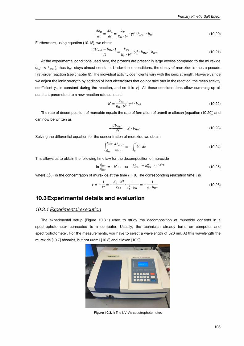
Primary Kinetic Salt Effect
103
𝑑𝑏𝑈𝑑𝑡
=𝑑𝑏𝐴𝑑𝑡
=𝑘23
𝐾𝐷 ∙ 𝑏0 ∙ 𝛾±
2 ∙ 𝑏𝑀𝑢− ∙ 𝑏𝐻+ (10.20)
Furthermore, using equation (10.18), we obtain
𝑑(𝑏𝑡𝑜𝑡 − 𝑏𝑀𝑢−)
𝑑𝑡=
𝑘23𝐾𝐷 ∙ 𝑏
0∙ 𝛾±
2 ∙ 𝑏𝑀𝑢− ∙ 𝑏𝐻+ (10.21)
At the experimental conditions used here, the protons are present in large excess compared to the murexide
(𝑏𝐻+ ≫ 𝑏𝑀𝑢−), thus 𝑏𝐻+ stays almost constant. Under these conditions, the decay of murexide is thus a pseudo
first-order reaction (see chapter 8). The individual activity coefficients vary with the ionic strength. However, since
we adjust the ionic strength by addition of inert electrolytes that do not take part in the reaction, the mean activity
coefficient 𝛾± is constant during the reaction, and so it is 𝛾±2. All these considerations allow summing up all
constant parameters to a new reaction rate constant
𝑘′ =𝑘23
𝐾𝐷 ∙ 𝑏0 ∙ 𝛾±
2 ∙ 𝑏𝐻+ (10.22)
The rate of decomposition of murexide equals the rate of formation of uramil or alloxan (equation (10.20)) and
can now be written as
−𝑑𝑏𝑀𝑢−
𝑑𝑡= 𝑘′ ∙ 𝑏𝑀𝑢− (10.23)
Solving the differential equation for the concentration of murexide we obtain
∫𝑑𝑏𝑀𝑢−
𝑏𝑀𝑢−
𝑏𝑀𝑢−𝑡
𝑏𝑀𝑢−0
= −∫ 𝑘′ ∙ 𝑑𝑡𝑡
0
(10.24)
This allows us to obtain the following time law for the decomposition of murexide
ln𝑏𝑀𝑢−𝑡
𝑏𝑀𝑢−0 = −𝑘′ ∙ 𝑡 or 𝑏𝑀𝑢−
𝑡 = 𝑏𝑀𝑢−0 ∙ 𝑒−𝑘
′∙𝑡 (10.25)
where 𝑏𝑀𝑢−0 is the concentration of murexide at the time 𝑡 = 0. The corresponding relaxation time 𝜏 is
𝜏 = −1
𝑘′= −
𝐾𝐷 ∙ 𝑏0
𝑘23∙
1
𝛾±2 ∙ 𝑏𝐻+
= −1
𝑘 ∙ 𝑏𝐻+ (10.26)
10.3 Experimental details and evaluation
10.3.1 Experimental execution
The experimental setup (Figure 10.3.1) used to study the decomposition of murexide consists in a
spectrophotometer connected to a computer. Usually, the technician already turns on computer and
spectrophotometer. For the measurements, you have to select a wavelength of 520 nm. At this wavelength the
murexide [10.7] absorbs, but not uramil [10.8] and alloxan [10.9].
Figure 10.3.1: The UV-Vis spectrophotometer.

Primary Kinetic Salt Effect
104
You need the following solutions:
Murexide solution: Prepare 100 mL solution of 36,6 mg of murexide in deionized water (molar
mass M = 284.19 g/mol).
Hydrochloric acid solution: 0,05 M, available in the laboratory
Ammonium chloride solution: 0.5 M, molar mass M = 53.49 g/mol, available in the laboratory
Deionized water
In the experiment, concentrations based on molarity (mol/L) and not molality (mol/kg) are used. Estimate the
difference between the two values and decide if it is negligible or not.
The first column in Table 10.3.1 corresponds to the reference used to calibrate, the spectrophotometer.
First, add the corresponding volumes of murexide solution, H2O and NH4Cl solution to the cuvette using a pipette.
Finally, add the acid and mix by briefly pipetting up and down. Then, put the cuvette into the cuvette holder and
start the measurement immediately.
Table 10.3.1: Scheme of the composition of each solutions to test. The numbers given are in mL of solution.
Solution Reference Solution 1 Solution 2 Solution 3 Solution 4 Solution 5
Murexide – 0,5 0,5 0,5 0,5 0,5
H2O 2,5 2,0 1,5 1,0 0,5 –
NH4Cl – – 0,5 1,0 1,5 2,0
HCl 1,0 1,0 1,0 1,0 1,0 1,0
Figure 10.3.2: The measuring program M.Wave.
The measuring program (Figure 10.3.2) records the transmittance 𝑇 vs. time 𝑡 in seconds.
The measurements will stop automatically after 𝑡 = 900 s. To save your data choose “Save” in the “File” menu.
For the file type use “Comma Separated Value File (*.csv)” (Figure 10.3.2).

Primary Kinetic Salt Effect
105
10.3.2 Data evaluation
From the transmittance 𝑇 vs. time 𝑡 in seconds. Calculate the absorbance 𝐴 from that, in time intervals
of minutes.
Plot ln 𝐴 vs. time 𝑡 for each solution and determine the relaxation time 𝜏 from the slope of the straight
line, according to equation (10.25) and (10.26).
Use the relaxation times to calculate the rate constant 𝑘′ for the different conditions, by using equation
(10.26).
Verify the Brønsted equation (10.14).
Perform an error analysis for all calculations. For the used spectrophotometer 𝛿𝑇 = 0.012 ∙ 𝑇
10.4 Applications of the experiment and its theory
In the case of reactions between large molecules (e.g., proteins) usually not all charges on the
interacting molecules do influence the reaction kinetics. Then, studying the effect of ionic strength on
the kinetics may reveal information on the charges that influence the reaction rate.
Murexide is the final product of the murexide-reaction, an analytical reaction to detect uric acid,
xanthine and other related substances.
Murexide can be used as an indicator since it undergoes a colour change in the presence of calcium
ions and other specific metal ions.
10.5 Literature
10.1 - P.W. Atkins, Physical Chemistry, 6th ed., Oxford University Press, Oxford (1998), pp. 819-837.
10.2 - P.W. Atkins and J. de Paula, Atkins’ Physical Chemistry, 8th ed., Oxford University Press, Oxford (2006),
pp. 880-885.
10.3 - P.W. Atkins, Physical Chemistry, 6th ed., Oxford University Press, Oxford (1998), pp. 249-253.
10.4 - P.W. Atkins and J. de Paula, Atkins’ Physical Chemistry, 8th ed., Oxford University Press, Oxford (2006),
pp. 163-165.
10.5 - P. Debye, and E. Hückel, Zur Theorie der Elektrolyte. I. Gefrierpunktserniedrigung und verwandte
Erscheinungen. Phys. Z. 24 (1923) 185-206.
10.6 - Eyring, H., The activated complex in chemical reactions. J. Chem. Phys. 3 (1935) 107-115.
10.7 - National Center for Biotechnology Information. PubChem Compound Database; CID=14453351,
https://pubchem.ncbi.nlm.nih.gov/compound/14453351 (accessed Aug. 12, 2016).
10.8 - National Center for Biotechnology Information. PubChem Compound Database; CID=67051,
https://pubchem.ncbi.nlm.nih.gov/compound/67051 (accessed Aug. 12, 2016).
10.9 - National Center for Biotechnology Information. PubChem Compound Database; CID=5781,
https://pubchem.ncbi.nlm.nih.gov/compound/5781 (accessed Aug. 12, 2016).

106
11 Estimation and Propagation of Measurement
Uncertainties
11.1 Basics and types of measurement uncertainties
Any measurement of a physical quantity is flawed by a measurement uncertainty (or error), no matter how
sophisticatedly the measurement procedure is designed. Since experimental data cannot be determined with
unlimited accuracy, a measurement, lacking information on its precision, is essentially useless. Therefore, in any
publication or report it is necessary to specify the uncertainty of the acquired result. This uncertainty is also called
measurement error and can either be given as an absolute error:
𝐸𝐴 = 110 ± 1.2kJ
mol (11.1)
or as a relative error:
𝐸𝐴 = 110 ± 1.1%kJ
mol (11.2)
Here 110 kJ/mol corresponds to an average value of the activation energy 𝐸𝐴̅̅ ̅ determined from a series of
measurements. 1.2 kJ/mole is the absolute error 𝛿𝐸𝐴 while 1.1% is the relative error 𝛿𝐸𝐴/𝐸𝐴̅̅ ̅. Units are essential
and you must not forget them.
Keep in mind the following meaning of any experimentally obtained result like 𝐸𝐴̅̅ ̅:
a) Usually, it is the arithmetic mean of a series of measurements and merely represents an approximation
of the true value (𝐸𝐴𝑡𝑟𝑢𝑒).
b) With a certain probability the true value 𝐸𝐴𝑡𝑟𝑢𝑒 lies within the interval [𝐸𝐴̅̅ ̅ − 𝛿𝐸𝐴, 𝐸𝐴̅̅ ̅ + 𝛿𝐸𝐴]. This probability
is called the confidence level or level of significance and usually is 68% (see below). The width of the
interval is determined by the size of the error 𝛿𝐸𝐴.
The significant digits in the measured value are the digits larger than or similar to the uncertainty. As a matter
of principle, the uncertainty of the error is of the same magnitude as the error itself, thus the uncertainty must not
indicate more than two significant digits. Accordingly, the experimental value must not indicate digits smaller than
the error (non-significant):
𝐸𝐴 = 110. 493826397⏟ 𝑛𝑜𝑛−𝑠𝑖𝑔𝑛𝑖−𝑓𝑖𝑐𝑎𝑛𝑡 𝑑𝑖𝑔𝑖𝑡𝑠
± 1.2263kJ
mol
If the error is not given explicitly, it is assumed that only significant digits are given and that its magnitude is half
of the last significant digit:
𝐸𝐴 = 110 = 110 ± 0.5 𝑘𝐽
𝑚𝑜𝑙
In the following paragraphs (11.1.1 to 11.1.3) the three main types of error (coarse, statistical and systematic
errors) are discussed.
11.1.1 Coarse errors
Coarse errors appear if the experiment exhibits fundamental uncertainties. Examples for sources of coarse
errors are:
Unsuitable experimental setup, e.g., characterized by uncontrolled parameters (not keeping the
measuring conditions like temperature and pressure constant).

Estimation and Propagation of Measurement Uncertainties
107
Unsuitable technique of measurement, e.g., trying to determine the temperature in a very small sample
(1cm3 of a liquid or a small amount of gas) using a thermometer having a large heat capacity.
Wrong calibration.
Wrong reading of the experimental data.
Deteriorated samples.
Rigorous planning of the experiment will avoid coarse errors:
Be familiar with theoretical background and literature relative to the experiment.
Estimate the expected magnitude of collected data and compare it with the precision of your equipment
before starting the experiment.
Perform control measurements with reference samples.
Be sure to have full control of every step of the experimental procedure.
11.1.2 Statistical errors
Increasing measurement precision of any physical quantity will progressively reveal fluctuations. Sophisticated
instruments and experimental setup may reduce such fluctuations. However, they are ultimately based on the
nature of thermodynamics (Boltzmann distribution) and thus are inevitable. Mainly, they lead to randomly
distributed measurement, having positive and negative deviations from the real value, that, due to their statistical
nature, have equal probability. Therefore, if the number of measurements is increased, they cancel each other in
a cumulative way. Thus, the statistical error of the average of a measured variable can be reduced, but not
infinitely, by increasing the amount of acquired data.
In order to determine the size of the statistical error the mean of the square of the error needs to be considered,
since this leads to a summation of just positive values that do not eliminate each other (see paragraph 11.2.1 for
the theory of statistical errors). Various possible sources of statistical errors are:
Reading error: the signal of an analog measuring instrument usually can only be determined with an
accuracy of half or quarter of the smallest separation of marks on the scale (think about a ruler with
millimeter graduation or an analog thermometer). A Vernier scale (German: Nonius-Skala, see Figure
10.5.1) may provide a significant improvement of this interpolation problem.
Figure 10.5.1: A vernier scale.
Error of digitalization: trivially, a digital measuring device can only be accurate up to the last specified
digit. However, beware because the error could be much larger than the last digit due to intrinsic noise of
the instrument or of the setup.

Estimation and Propagation of Measurement Uncertainties
108
Environmental influences: vibrations, fluctuations of temperature (feedback fluctuations of a
thermostat), alternating electrical field (pick-up).
Shot noise: (German: Schrotrauschen): Some physical properties are “quantized”, i.e., the minimal unit
electrical charge is the electron charge, or the smallest unit of light energy is that of a photon ℎ∙𝑐
𝜆. Single
charges can be detected by an electron multiplier (like in a mass spectrometer), single photons can be
counted using a Geiger counter (measuring radioactive decay) or a photomultiplier (e.g., in fluorimeter).
Therefore such quantities can only be detected as an integer multiple of the unit quantity.
Intrinsic noise (fluctuations): based on the quantum nature of charge, any electronic component (e.g., a
resistor) exhibits an unavoidable basic noise current (Nyquist noise, Figure 10.5.2A). Any amplification of
the signal will also amplify this noise (like for the sizzling noise in an audio amplifier that is completely
turned up in the absence of an input signal). Usually, the intrinsic noise has a characteristic frequency
response: the larger the frequency, the smaller the amplitude of the noise (1/f noise, Figure 10.5.2B).
Figure 10.5.2: A) Noise current as a function of time; B) Intensity of the noise current as a function of frequency.
As mentioned above, ultimately any physical quantity exhibits statistical errors due to thermal agitation of
particles reflected in the Boltzmann distribution (or Fermi- and Bose-Einstein distribution). The higher the
temperature the broader the distribution. An exciting example of maximum reduction of thermal noise by cooling
down electronic amplifiers to a temperature of 4.2 K is given in Figure 10.5.3.
Figure 10.5.3: Output signal of an amplifier of the receiving earth station in Raisting (Bavaria, Germany). The receiving station is cooled down to 4.2 K and exhibits a noise amplitude of 10-14 A. This noise can further be reduced to 5∙10-17 A by averaging the
signal over one hour (this noise current corresponds to a fluctuation 300 electrons per second).
In summary: in order to minimize statistical errors, it is necessary to perform measurements repeatedly and
to obtain average values of these data (see paragraph 11.2).

Estimation and Propagation of Measurement Uncertainties
109
11.1.3 Systematic errors
Under identical measuring conditions, systematic errors impair the measurement always in a similar manner.
On repeating the measurement, the value and sign of a systematic error remain the same and therefore it cannot
be reduced by averaging.
Possible origins of systematic errors are:
Air buoyancy on weight.
Temperature dependence of practically all physical quantities (e.g., expansion of a ruler with increasing
temperature).
External electrical d.c. fields.
Instability of samples and measuring setups due to ageing.
Wrong zero point: many measuring devices do not report the exact zero point and therefore all measured
data are shifted by a certain value, e.g., in balances, shifted scales, parallax errors.
Friction and Hysteresis effects: when measurement series at increasing pressure and decreasing pressure
reveal different data.
Non-linearity: most measuring sensors are based on idealized linear physical laws. However, on closer
inspection one usually finds deviations from linearity, especially if the measuring parameters become
large. Examples are: Hooke’s law in a spring balance, ideal gas law in gas thermometers, non-linear
distortions in analog-digital converters.
Strategies to minimize systematic errors are:
Providing a reliable and accurate experimental setup. Counteracting systematic deviations can be utilized
for mutual compensation.
Experimental and theoretical calibration functions can be utilized for numerical corrections.
Different measuring methods could be compared.
In summary: generally, it is not possible to account for systematic errors within the context of a practical
course. However, a discussion of possible sources of systematic error can be carried out.
11.1.4 Precision and accuracy
The statistical error reflects the precision of a measurement, meaning its reproducibility. Only if the systematic
error is small as well, the result of a measurement will be close to the corresponding real value and is thus accurate
(Figure 11.1.4).
Figure 10.5.4: Precision and accuracy of a determined measuring parameter.
The following paragraph 11.2 describe the statistical methods that are used in order to quantify the precision
of a measurement.

Estimation and Propagation of Measurement Uncertainties
110
11.2 Quantification of the precision of a measurement
11.2.1 Mean value and statistical error
An example of data collection is: with a stopwatch with a display accuracy of 0.01 s, we measure the time ti
needed for a steel bullet to fall from the lowest viewing platform of the Munich’s Olympia tower (height: 172 m).
Table 10.5.1 shows 20 individual measurements.
Table 10.5.1: Data sheet for 20 individual measurements of the falling time taken from a steel bullet falling from the Munich’s Olympia tower.
No. of measurement (= index i)
𝑡𝑖 (s) Deviation from the mean
value: 𝑡𝑖 − 𝑡̅ (s) (𝑡𝑖 − 𝑡̅)2 (s²)
1 5.51 -0.02 0.0006
2 5.26 -0.28 0.0761
3 5.04 -0.49 0.2430
4 5.63 0.10 0.0095
5 5.39 -0.14 0.0204
6 5.83 0.30 0.0902
7 6.01 0.48 0.2282
8 5.64 0.11 0.0124
9 5.06 -0.47 0.2205
10 5.18 -0.35 0.1222
11 5.75 0.22 0.0467
12 5.72 0.19 0.0367
13 5.94 0.40 0.1633
14 5.69 0.16 0.0244
15 5.49 -0.04 0.0014
16 5.74 0.2 0.0445
17 5.70 0.17 0.0287
18 5.32 -0.22 0.0466
19 5.42 -0.11 0.0125
20 5.32 -0.22 0.0463
Sum: 110.62 -0.0000000000000133 1.4742
The arithmetic mean value 𝑡̅ of the falling time is calculated according to
𝑡̅ =1
𝑛∙∑𝑡𝑖
𝑛
𝑖=1
=110.62 𝑠
20= 5.53 𝑠 (11.3)
Calculating the average of the deviation of the individual falling times from its mean value, positive and negative
terms (in the third column of Table 10.5.1) cancel each other, the small value that remains (-0.0000000000000133)
results from rounding errors of the software program:
1
𝑛∙∑(𝑡𝑖 − 𝑡̅)
𝑛
𝑖=1
= 0.0000000000000133 ≈ 0 (11.4)
As one can easily prove, the deviation is exactly zero:
(𝑡𝑖 − 𝑡̅)̅̅ ̅̅ ̅̅ ̅̅ ̅̅ =1
𝑛∙∑(𝑡𝑖 − 𝑡̅) =
𝑛
𝑖=1
1
𝑛∙∑(𝑡𝑖) −
1
𝑛∙∑(𝑡̅)
𝑛
𝑖=1
= 𝑡̅ −1
𝑛∙ 𝑛 ∙ 𝑡̅ =
𝑛
𝑖=1
0 (11.5)

Estimation and Propagation of Measurement Uncertainties
111
In order to determine the size of the statistical error (i.e., to quantify the average magnitude of deviation) Gauss
(and Legendre) suggested to average the squares of the deviations (𝑡𝑖 − 𝑡̅)2 (fourth column of Table 10.5.1). In
this way, the standard deviation 𝜎 of the individual measurement is calculated by averaging the squares of the
errors. This leads to a summation of just positive values that do not eliminate each other.
𝜎 = √1
𝑛 − 1∙∑(𝑡𝑖 − 𝑡̅)2
𝑛
𝑖=1
= 0.278 𝑠 (11.6)
The square of equation (11.6) 𝜎2, is called variance.
Note: In equation (11.6), the mean value 𝑡̅ is assumed to be known and by this it determines one of the 𝑛 terms
(𝑡𝑖 − 𝑡̅)2. Thus, there exist only 𝑛 − 1 independent terms. Therefore the sum is divided by 𝑛 − 1 (however, in
general, 𝑛 − 1 ≈ 𝑛).
11.2.1.1 Gauss’s least-squares method
In principle, there are various ways of averaging data, the most natural and simple is the arithmetic mean as
in equation (11.3). Carl Friedrich Gauss pointed out, that the arithmetic mean value has a unique and important
property. If you look at the square of the deviations of all the data points 𝑥𝑖 from any mean value: (�̅� − 𝑥𝑖)2 one
finds, that the sum of all these squares ∑ (�̅� − 𝑥𝑖)2𝑛
𝑖=1 is minimal only if �̅� is an arithmetic mean according to
equation (11.3).
11.2.2 Probability distribution
The scattering of individual measuring values can easily be captured in a probability distribution and depicted
as a histogram (bar plot). To construct a histogram, the first step is to define the range of values, i.e., divide the
entire range of values into a series of intervals [𝑡𝑘 −1
2Δ𝑡, 𝑡𝑘 +
1
2Δ𝑡] (called classes) and then count how many values
fall into each interval (called frequency of occurrence 𝑛𝑘). Here the horizontal axis (abscissa) shows the falling
time 𝑡, the vertical axis (ordinate) gives 𝑛𝑘. Figure 10.5.5 shows the probability distribution derived from the data
of Table 10.5.1 (with 𝑛 = 20 and an interval width of 𝑡 = 0.2 s).
Figure 10.5.5: Histogram of the data given in Table 10.5.1 using an interval width of 𝑡 = 0.2 s, leading to six individual classes.
This distribution has a centroid exactly at the arithmetic mean value 𝑡̅ = 5.53 s. However, due to the small
number of data, the distribution is ill defined. The width of the distribution is a measure of the scatter of the data
points and is given by the standard deviation = 0.278s. If we increase the number of data points, we observe,
that the distribution becomes smoother and better defined (see Figure 10.5.6), while both centroid and width are

Estimation and Propagation of Measurement Uncertainties
112
independent from the number of measurements; depicts the quality of each individual measurement. On the
other hand, it is obvious that the distribution would become imperceptible, if the number of data points would be
considerably smaller than 𝑛 = 20.
Usually, it makes sense to normalize distributions to handle them easily and to compare different distributions
with each other. For normalization, the frequency 𝑓𝑘 (relative probability or probability density) is introduced; it
corresponds to the probability of finding a measuring value in a certain interval [𝑡𝑘 −1
2Δ𝑡, 𝑡𝑘 +
1
2Δ𝑡] and it is given
by
𝑓𝑘 =𝑎𝑏𝑠𝑜𝑙𝑢𝑡𝑒 𝑝𝑟𝑜𝑏𝑎𝑏𝑖𝑙𝑖𝑡𝑦 𝑛𝑘
𝑛𝑢𝑚𝑏𝑒𝑟 𝑜𝑓 𝑚𝑒𝑎𝑠𝑢𝑟𝑒𝑚𝑒𝑛𝑡𝑠 𝑛=
𝑛𝑘∑ 𝑛𝑘𝐾𝑘=1
(11.7)
This normalization provides that the sum of all 𝑓𝑘 is 1 (=100%)
In order to make the depicted distribution independent by the interval width Δ𝑡, the relative probability 𝑓𝑘 is
further divided by Δ𝑡 to reveal the probability density 𝑟𝑘 (see Figure 10.5.6)
𝑟𝑘 = 𝑓𝑘Δ𝑡
(11.8)
Applying equation (11.8) to a given probability density makes possible to calculate back the frequency of finding
a measuring result in an arbitrary interval [𝑡𝑘 −1
2Δ𝑡, 𝑡𝑘 +
1
2Δ𝑡]
𝑓𝑘 = 𝑟𝑘 ∙ Δ𝑡 (11.9)
In a histogram the number of classes 𝐾 depends on the interval size ∆𝑡 and on the length of the horizontal axis
𝑡𝑚𝑎𝑥 − 𝑡𝑚𝑖𝑛 = 𝐾 ∙ ∆𝑡. Here 𝐾 = 15. The proper choice of 𝐾 is not trivial and depends on the number of data 𝑛,
which are available. If 𝐾 is chosen too large, the noise in each interval will be too large, if 𝐾 is too small, the
diagram will be too coarse. It is good practice to choose
𝐾 ≈ √𝑛 for 𝑛 ≤ 1000 (11.10)
𝐾 ≈ 10 log 𝑛 for 𝑛 > 1000 (11.11)
Figure 10.5.6: Normalized frequency (probability density) for 200 measuring values of the falling time of a steel bullet from Munich’s Olympia tower using 𝑡 = 0.1s leading to K = 15. The pink line represents the corresponding continuous Gaussian distribution (𝑡) (see paragraph 11.2.3).
Moving on to the limiting case of an infinite number of measurements leads to infinitesimal intervals ∆𝑡 and the
discrete distribution becomes a continuous function, called limiting distribution (𝑡).
Mean value:
𝑡̅ = 5.53 s
Width: σ = 0.278 s
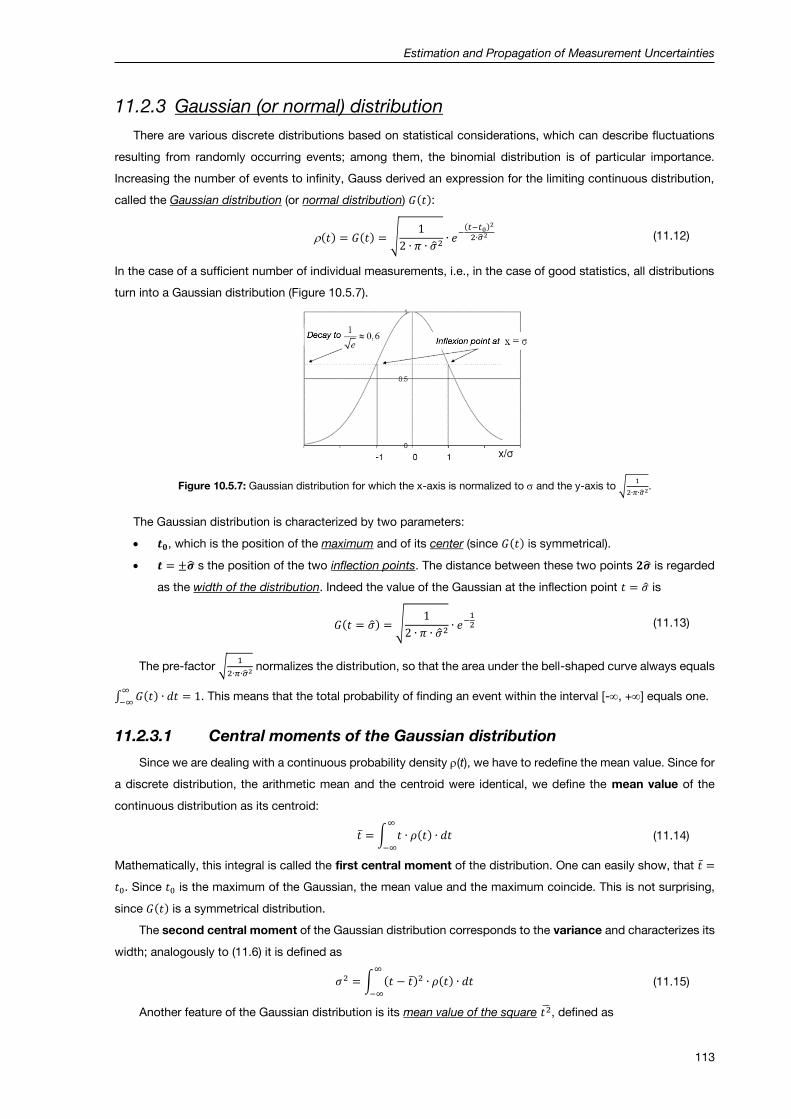
Estimation and Propagation of Measurement Uncertainties
113
11.2.3 Gaussian (or normal) distribution
There are various discrete distributions based on statistical considerations, which can describe fluctuations
resulting from randomly occurring events; among them, the binomial distribution is of particular importance.
Increasing the number of events to infinity, Gauss derived an expression for the limiting continuous distribution,
called the Gaussian distribution (or normal distribution) 𝐺(𝑡):
(𝑡) = 𝐺(𝑡) = √1
2 ∙ 𝜋 ∙ �̂�2∙ 𝑒
−(𝑡−𝑡0)
2
2∙�̂�2 (11.12)
In the case of a sufficient number of individual measurements, i.e., in the case of good statistics, all distributions
turn into a Gaussian distribution (Figure 10.5.7).
Figure 10.5.7: Gaussian distribution for which the x-axis is normalized to and the y-axis to √1
2∙𝜋∙�̂�2.
The Gaussian distribution is characterized by two parameters:
𝒕𝟎, which is the position of the maximum and of its center (since 𝐺(𝑡) is symmetrical).
𝒕 = ±�̂� s the position of the two inflection points. The distance between these two points 𝟐�̂� is regarded
as the width of the distribution. Indeed the value of the Gaussian at the inflection point 𝑡 = �̂� is
𝐺(𝑡 = �̂�) = √1
2 ∙ 𝜋 ∙ �̂�2∙ 𝑒−
12 (11.13)
The pre-factor √1
2∙𝜋∙�̂�2 normalizes the distribution, so that the area under the bell-shaped curve always equals
∫ 𝐺(𝑡) ∙ 𝑑𝑡 = 1∞
−∞. This means that the total probability of finding an event within the interval [-, +] equals one.
11.2.3.1 Central moments of the Gaussian distribution
Since we are dealing with a continuous probability density (t), we have to redefine the mean value. Since for
a discrete distribution, the arithmetic mean and the centroid were identical, we define the mean value of the
continuous distribution as its centroid:
𝑡̅ = ∫ 𝑡 ∙ 𝜌(𝑡) ∙ 𝑑𝑡∞
−∞
(11.14)
Mathematically, this integral is called the first central moment of the distribution. One can easily show, that 𝑡̅ =
𝑡0. Since 𝑡0 is the maximum of the Gaussian, the mean value and the maximum coincide. This is not surprising,
since 𝐺(𝑡) is a symmetrical distribution.
The second central moment of the Gaussian distribution corresponds to the variance and characterizes its
width; analogously to (11.6) it is defined as
𝜎2 = ∫ (𝑡 − 𝑡̅)2 ∙ 𝜌(𝑡) ∙ 𝑑𝑡∞
−∞
(11.15)
Another feature of the Gaussian distribution is its mean value of the square 𝑡2̅, defined as
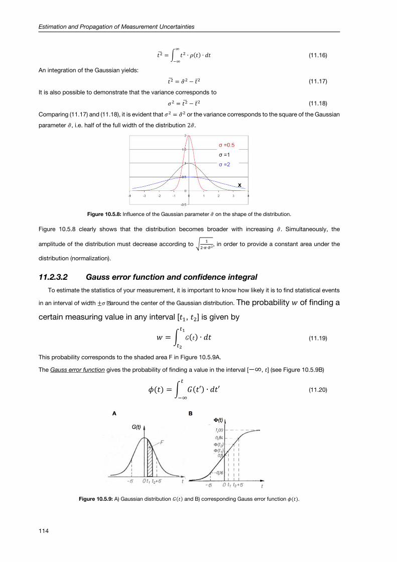
Estimation and Propagation of Measurement Uncertainties
114
𝑡2̅ = ∫ 𝑡2 ∙ 𝜌(𝑡) ∙ 𝑑𝑡∞
−∞
(11.16)
An integration of the Gaussian yields:
𝑡2̅ = �̂�2 − 𝑡̅2 (11.17)
It is also possible to demonstrate that the variance corresponds to
𝜎2 = 𝑡2̅ − 𝑡̅2 (11.18)
Comparing (11.17) and (11.18), it is evident that 𝜎2 = �̂�2 or the variance corresponds to the square of the Gaussian
parameter �̂�, i.e. half of the full width of the distribution 2�̂�.
Figure 10.5.8: Influence of the Gaussian parameter �̂� on the shape of the distribution.
Figure 10.5.8 clearly shows that the distribution becomes broader with increasing �̂�. Simultaneously, the
amplitude of the distribution must decrease according to √1
2∙𝜋∙�̂�2, in order to provide a constant area under the
distribution (normalization).
11.2.3.2 Gauss error function and confidence integral
To estimate the statistics of your measurement, it is important to know how likely it is to find statistical events
in an interval of width ±𝜎 around the center of the Gaussian distribution. The probability 𝑤 of finding a
certain measuring value in any interval [𝑡1, 𝑡2] is given by
𝑤 = ∫ 𝐺(𝑡) ∙ 𝑑𝑡𝑡1
𝑡2
(11.19)
This probability corresponds to the shaded area F in Figure 10.5.9A.
The Gauss error function gives the probability of finding a value in the interval [−∞, 𝑡] (see Figure 10.5.9B)
𝜙(𝑡) = ∫ 𝐺(𝑡′) ∙ 𝑑𝑡′𝑡
−∞
(11.20)
Figure 10.5.9: A) Gaussian distribution 𝐺(𝑡) and B) corresponding Gauss error function 𝜙(𝑡).

Estimation and Propagation of Measurement Uncertainties
115
Since 𝜙(𝑡) is the primitive function of 𝐺(𝑡), the probability 𝑤 in (11.19) can be easily calculated from the difference
𝜙(𝑡2) − 𝜙(𝑡1). Unfortunately, 𝜙(𝑡) cannot be integrated analytically and we have to use tables given in
mathematical formularies. The probability 𝑤𝜎 of finding a measuring value within the interval [𝑡0 − 𝜎, 𝑡0 + 𝜎] can
be quantified as
𝑤𝜎 = ∫ ∙ 𝐺(𝑡) ∙ 𝑑𝑡 = 𝜙(𝜎) − 𝜙(−𝜎) = 0.841 − 0.159 = 0.683 = 68.3%𝑡0+𝜎
𝑡0−𝜎
(11.21)
In physics the above-mentioned interval of a single standard deviation from the maximum of the distribution [𝑡0 −
𝜎, 𝑡0 + 𝜎] is generally accepted as the confidence interval.
In the technical field, a higher safety is required; therefore, the confidence interval is extended to ± the doubled
standard deviation [𝑡0 − 2𝜎, 𝑡0 + 2𝜎]. The probability of finding the measuring values in this region increases to
95.5%. In biology and medicine, the criterion of confidence is further enhanced to a probability of 97.7%, which
is reached in the interval [𝑡0 − 3𝜎, 𝑡0 + 3𝜎].
11.3 Error propagation
In most experiments, there is more than one measurement to carry out and we have to calculate the desired
result with the help of a physical formula. For example, in order to determine the gravitational constant from 𝑔 =
2∙ℎ̅
𝑡̅2, we have to measure both the falling time 𝑡 and the height ℎ. From both measurements, we get average values
𝑡̅ and ℎ̅ with different accuracies, defined by the standard deviations 𝜎𝑡 and 𝜎ℎ.
The crucial question now is: how can we determine the best value for 𝑔 and what is the accuracy and precision
of the obtained result? Generally speaking, we want to determine the value of a physical quantity 𝑓, which is a
function of the measurable parameters 𝑓(𝑥1, 𝑥2, 𝑥3…), having uncertainties (∆𝑥1, ∆𝑥2, ∆𝑥3…). Our task is to obtain
a meaningful result from the function 𝑓(𝑥1, 𝑥2, 𝑥3…) and to track the propagation of the measurement uncertaities,
(∆𝑥1, ∆𝑥2, ∆𝑥3…) on the accuracy and precision of the result. To do so, it is necessary to discriminate between
systematic errors and statistical errors.
11.3.1 Propagation of systematic errors
A systematic uncertainty of a measurement is not random, i.e., it has a distinct tendency. If we make a Taylor
expansion of our function 𝑓:
𝑓(𝑥1 + ∆𝑥1, 𝑥2 + ∆𝑥2, … ) = 𝑓(𝑥1, 𝑥2, … ) +∑(𝜕𝑓
𝜕𝑥𝑖) ∙ ∆𝑥𝑖
𝑁
𝑖=1
+ ∑ (𝜕𝑓
𝜕𝑥𝑖) (
𝜕𝑓
𝜕𝑥𝑘) ∙ ∆𝑥𝑖 ∙ ∆𝑥𝑘
𝑁
𝑖,𝑘=1
+⋯ (11.22)
the systematic error ∆𝑓𝑠𝑦𝑠𝑡 can be calculated as
∆𝑓𝑠𝑦𝑠𝑡(𝑥1, 𝑥2, … ) = 𝑓(𝑥1 + ∆𝑥1, 𝑥2 + ∆𝑥2, … ) − 𝑓(𝑥1, 𝑥2, … ) =∑(𝜕𝑓
𝜕𝑥𝑖) ∙ ∆𝑥𝑖
𝑁
𝑖=1
(11.23)
Since usually the errors are small, the expansion in equation (11.22) is truncated at the linear term. For this reason,
systematic errors contribute to the final error ∆𝑓𝑠𝑦𝑠𝑡 in a linear way.
11.3.2 Gaussian propagation of statistical errors
11.3.2.1 Functions of a single variable
For simplicity we first discuss a simple example with only a single measured parameter and a quadratic
function 𝑓(𝑥) = 𝑎 ∙ 𝑥2. In Figure 10.5.10, a Gaussian distribution of 𝑥 is depicted in the horizontal axis with a mean
value �̅� and an error ∆𝑥 (i.e., standard deviation 𝜎), corresponding to the width of the distribution. From each

Estimation and Propagation of Measurement Uncertainties
116
value of 𝑥 we can calculate a result 𝑓(𝑥) and construct a distribution of results (depicted on the vertical axis). Note
that the new distribution is not symmetric anymore, because of the rising slope of the function 𝑓(𝑥). With this
distribution of 𝑓𝑖 values it is possible to calculate the average value 𝑓(𝑥)̅̅ ̅̅ ̅̅ . Having more than one parameter 𝑥, this
procedure becomes tedious and impractical.
Figure 10.5.10: Formation of the real mean value 𝑓(𝑥)̅̅ ̅̅ ̅̅ in the case of strong non-linearity. The mean value 𝑓(𝑥)̅̅ ̅̅ ̅̅ is shifted towards higher values since the distribution of the 𝑓𝑖 values is asymmetric. Furthermore, the width of the distribution of the 𝑓𝑖 values becomes larger.
Obviously, it would be much simpler to average over the 𝑥𝑖 values first, obtaining �̅�, and to calculate 𝑓(�̅�) in a
second step. The question will be whether such a procedure is appropriate, and in particular, how large the error
will be.
To investigate this issue we construct a linear approximation the function 𝑓(𝑥) = 𝑎 ∙ 𝑥2 by making a Taylor
expansion in terms of a deviation ∆𝑥 around the mean value of �̅�, as we did in paragraph 11.3.1:
𝑓(�̅� + ∆𝑥) = 𝑓(�̅�) +∑(𝜕𝑓
𝜕𝑥𝑖) ∙ ∆𝑥𝑖
𝑁
𝑖=1
+ ∑ (𝜕𝑓
𝜕𝑥𝑖) (
𝜕𝑓
𝜕𝑥𝑘) ∙ ∆𝑥𝑖 ∙ ∆𝑥𝑘
𝑁
𝑖,𝑘=1
+⋯ (11.24)
Neglecting the higher-order terms and in the case of the quadratic function 𝑓(𝑥) = 𝑎 ∙ 𝑥2 we can derive:
𝑓(�̅� + ∆𝑥) = 𝑓(�̅�) +∑(𝜕𝑓
𝜕𝑥𝑖) ∙ ∆𝑥𝑖
𝑁
𝑖=1
= 𝑎 ∙ �̅�2 + 2𝑎 ∙ �̅� ∙ ∆𝑥 (11.25)
This approximation of 𝑓(𝑥)̅̅ ̅̅ ̅̅ as a linear function of ∆𝑥 is shown in Figure 10.5.11 as a dashed red line touching the
correct function 𝑓(𝑥) as a tangent at �̅�. To construct the distribution of 𝑓𝑖 values, we simply have to mirror the
Gaussian distribution of the 𝑥 values at the dashed red tangent and obtain a Gaussian distribution of 𝑓𝑖 values.
Due to the symmetry of both distributions, the mean values 𝑓(𝑥)̅̅ ̅̅ ̅̅ and 𝑓(�̅�) coincide. Furthermore, we see how the
width of the distribution of 𝑥𝑖 affects the width of the 𝑓(𝑥) distribution: the larger the slope of the linear
approximation is, the larger the width of the 𝑓(𝑥) distribution will be.

Estimation and Propagation of Measurement Uncertainties
117
Figure 10.5.11: Construction of the distribution of 𝑓(𝑥) on the basis of a linear approximation of 𝑓(𝑥) = 𝑎 ∙ 𝑥2.
Frequently we are confronted with functions 𝑓(𝑥1, 𝑥2, 𝑥3…) of more than one independent variables 𝑥1, 𝑥2, 𝑥3….
In appendix, it is shown that:
1. The mean values 𝑓(𝑥1, 𝑥2, 𝑥3…)̅̅ ̅̅ ̅̅ ̅̅ ̅̅ ̅̅ ̅̅ ̅̅ ̅̅ ̅ and 𝑓(𝑥�̅�) = 𝑓(𝑥1̅̅ ̅, 𝑥2̅̅ ̅, … , 𝑥𝑁̅̅̅̅ ) coincide (see Appendix 11.5.1).
2. The Gaussian law of error propagation gives the statistical error of the result 𝑓(𝑥1, 𝑥2, 𝑥3…)̅̅ ̅̅ ̅̅ ̅̅ ̅̅ ̅̅ ̅̅ ̅̅ ̅̅ ̅ (see Appendix
11.5.2) as in:
𝜎𝑓 = √(𝜕𝑓
𝜕𝑥1)2
∙ 𝜎12 + (
𝜕𝑓
𝜕𝑥2)2
∙ 𝜎22 +⋯ (11.26)
Note:
i. Equation (11.26) is valid for statistical errors only.
ii. the error contributions of the individual measuring variables ∆𝑓1 = (𝜕𝑓
𝜕𝑥1)2∙ 𝜎1
2, ∆𝑓2 = (𝜕𝑓
𝜕𝑥2)2∙ 𝜎2
2,… do
not sum up linearly but partially compensate each other. This is considered in the orthogonal addition
(compare to the Pythagorean theorem, Figure 10.5.12).
iii. Only contributions that are similar in size are important, meaning that small contributions can be
neglected.
Figure 10.5.12: Pythagorean Theorem applied to the combination of the errors of two variables.
11.3.3 Useful rules for Gaussian error propagation
We now determine the derivatives for some frequently occurring functions and derive the Gaussian error
propagation.
11.3.3.1 Sum or difference of variables: 𝒇 = 𝒙𝟏 + 𝒙𝟐 or 𝒇 = 𝒙𝟏 − 𝒙𝟐
𝜎𝑓 = √(𝜕(𝒙𝟏 ± 𝒙𝟐)
𝜕𝑥1)2
∙ 𝜎12 + (
𝜕(𝒙𝟏 ± 𝒙𝟐)
𝜕𝑥2)2
∙ 𝜎22⇒ 𝜎𝑓 = √𝜎1
2 + 𝜎22 (11.27)
since (𝜕(𝒙𝟏±𝒙𝟐)
𝜕𝑥1)2= (
𝜕(𝒙𝟏±𝒙𝟐)
𝜕𝑥2)2= 1

Estimation and Propagation of Measurement Uncertainties
118
The error square of a sum or a difference equals the sum of the error squares of all summands.
11.3.3.2 Product or quotient of variables: 𝒇 = 𝒙𝟏 ∙ 𝒙𝟐 or 𝒇 =𝒙𝟏
𝒙𝟐
𝜎𝑓 = √(𝜕(𝒙𝟏 ∙ 𝒙𝟐)
𝜕𝑥1)2
∙ 𝜎12 + (
𝜕(𝒙𝟏 ∙ 𝒙𝟐)
𝜕𝑥2)2
∙ 𝜎22⇒ 𝜎𝑓 = √𝑥2
2 ∙ 𝜎12 + 𝑥1
2 ∙ 𝜎22 (11.28)
since (𝜕(𝒙𝟏∙𝒙𝟐)
𝜕𝑥1)2= 𝑥2
2 and (𝜕(𝒙𝟏∙𝒙𝟐)
𝜕𝑥2)2= 𝑥1
2.
Dividing by 𝐟 = 𝐱𝟏 ∙ 𝐱𝟐 reveals the relative error
𝜎𝑓
𝒇= √(
𝒙𝟐𝒙𝟏 ∙ 𝒙𝟐
)2
∙ 𝜎12 + (
𝒙𝟏𝒙𝟏 ∙ 𝒙𝟐
)2
∙ 𝜎22 = √(
𝜎1𝑥1)2
+ (𝜎2𝑥2)2
(11.29)
It is easy to demonstrate that equation (11.29) is valid also in the case of 𝐟 =𝐱𝟏
𝐱𝟐
The square of the relative error of a product or quotient equals the sum of the relative error squares of all
factors.
11.3.3.3 Exponential function: 𝒇 = 𝒙𝒏
𝜎𝑓 = √(𝜕𝑥𝑛
𝜕𝑥)2
∙ 𝜎𝑥2 (11.30)
Here 𝜕𝑥𝑛
𝜕𝑥= 𝑛 ∙ 𝑥𝑛−1. Dividing by 𝐟 = 𝐱𝐧 reveals the relative error:
𝜎𝑓
𝑓= √(
𝑛 ∙ 𝑥𝑛−1
𝐱𝐧)
2
∙ 𝜎𝑥2 = 𝑛 ∙
𝜎𝑥𝑥
(11.31)
The relative error of an exponential function equals the product of the relative error of the basis 𝑥 multiplied
by the exponent 𝑛
11.3.3.4 Natural exponential function: 𝒇 = 𝒆𝒂∙𝒙
𝜎𝑓 = √(𝜕𝐞𝐚∙𝐱
𝜕𝑥)2
∙ 𝜎𝑥2 (11.32)
Here 𝜕𝐞𝐚∙𝐱
𝜕𝑥= 𝑎 ∙ 𝐞𝐚∙𝐱. Dividing by 𝐟 = 𝐞𝐚∙𝐱 reveals the relative error:
𝜎𝑓
𝑓= √(
𝑎 ∙ 𝒆𝒂∙𝒙
𝒆𝒂∙𝒙)2
∙ 𝜎𝑥2 = 𝑎 ∙ 𝜎𝑥 (11.33)
The relative error of a natural exponential function equals the product of the absolute error of the basis x
multiplied by the coefficient at exponent 𝑎.
11.3.3.5 General and natural logarithms: 𝒇 = 𝐥𝐨𝐠𝒃 𝒙 and 𝒇 = 𝐥𝐧 𝒙
𝜎𝑓 = √(𝜕 log𝒃 𝒙
𝜕𝑥)2
∙ 𝜎𝑥2 = √(
1
𝑥 ∙ ln 𝑏)2
∙ 𝜎𝑥2 =
1
ln 𝑏∙𝜎𝑥𝑥
(11.34)
It is easy to demonstrate that 𝐟 = ln 𝐱 is a particular case of equation (11.34):
𝜎𝑓 = √(𝜕 ln 𝑥
𝜕𝑥)2
∙ 𝜎𝑥2 = √(
1
𝑥)2
∙ 𝜎𝑥2 =
𝜎𝑥𝑥
(11.35)
The absolute error of the logarithm of 𝑥 in base 𝑏 equals the relative error of 𝑥 multiplied by 1
𝑙𝑛 𝑏.

Estimation and Propagation of Measurement Uncertainties
119
11.3.4 Standard deviation of the mean value
Table 10.5.1 provides the data for the time 𝑡𝑖 of a steel bullet falling a certain distance. The experiment was
repeated 𝑛 times and from the 𝑛 𝑡𝑖 values the corresponding mean value 𝑡̅ (Equation (11.3)) and the standard
deviation 𝜎 of the individual measurements (Equation (11.6)) were determined. Comparing different data sets
would yield slightly different mean values 𝑡̅. This leads to the question of how the mean values (also called
optimum values) of different data sets deviate from each other, and in particular how much they deviate from the
“real value”. Though the real value is not known, it would be at the center of an idealized Gaussian distribution:
𝑡𝑟𝑒𝑎𝑙 = 𝑡0. We can formulate the standard deviation of the mean value 𝜎𝑚 (or the variance 𝜎𝑚2 of 𝑡̅ with respect
to 𝑡0) by its second moment:
𝜎𝑚2 = ∫ (𝑡̅ − 𝑡0)
2 ∙ 𝜌(𝑡) ∙ 𝑑𝑡∞
−∞
(11.36)
We can insert equation (11.3) in (11.36): 𝜎𝑚2 = ∫ (
1
𝑛∑ 𝑡𝑖 − 𝑡0𝑛𝑖=1 )2 ∙ 𝜌(𝑡) ∙ 𝑑𝑡
∞
−∞
𝜎𝑚2 = ∫ (
1
𝑛∑𝑡𝑖 − 𝑡0
𝑛
𝑖=1
)
2
∙ 𝜌(𝑡) ∙ 𝑑𝑡∞
−∞
(11.37)
Considering 𝑡̅ as a function of the individual measuring values 𝑡𝑖, each of which is affected by the error 𝜎. The
error of 𝑡̅, can be calculated according to Gaussian error propagation, obtaining:
𝜎𝑚2 = ∑ (
𝜕𝑡̅
𝜕𝑡𝑘)2
∙ 𝜎𝑘2𝑁
𝑘=1 where 𝜕𝑡̅
𝜕𝑡𝑘=
𝜕
𝜕𝑡𝑘(1
𝑛∙ ∑ 𝑡𝑖
𝑛𝑖=1 ) =
1
𝑛∙ ∑
𝜕
𝜕𝑡𝑘𝑡𝑖
𝑛𝑖=1 (11.38)
Since the derivative of independent variables is: 𝜕𝑡𝑖
𝜕𝑡𝑘= 1 for 𝑖 = 𝑘 and
𝜕𝑡𝑖
𝜕𝑡𝑘= 0 for 𝑖 ≠ 𝑘, the sum reduces to
∑𝜕
𝜕𝑡𝑘𝑡𝑖
𝑛𝑖=1 = 1, and we obtain:
𝜕𝑡̅
𝜕𝑡𝑘=
1
𝑛.
Since the standard deviation of each individual measurement remains constant, i.e. 𝜎𝑘 = 𝜎 we finally obtain:
𝜎𝑚2 = ∑(
1
𝑛)2
∙ 𝜎2𝑛
𝑘=1
=1
𝑛∙ 𝜎2 (11.39)
Taking the square root of (11.39), we get the simple but important result for the standard deviation of the
mean value:
𝜎𝑚 ==𝜎
√𝑛 (11.40)
Equation (11.40) clearly shows that the larger the data set, (the larger 𝑛) is, the smaller the standard deviation
of the mean value. For example, for 𝑛 = 10 ⇒ 𝜎𝑚 =𝜎
3.16 and for 𝑛 = 100 ⇒ 𝜎𝑚 =
𝜎
10.
11.4 Least square fitting
We want to discuss now whether the measuring values do obey a particular physical law or, if there´s no
physical model yet obtainable, whether the data can be reasonably described empirically by an analytical function
and how the parameters of the particular law can be optimized (search for the “best” curve = line of best fit or
regression line).
Let us describe the physical law by a function: 𝑦 = 𝑓( 𝑥1 , 𝑥, …2 𝛼1, 𝛼2, … ). Here, the dependent variable 𝑦 is
expressed by the variables 𝑥1 , 𝑥, …2 . Both 𝑦 and 𝑥𝑘 can be measured while the unknown parameters of theory
𝛼1…𝛼𝑗 …𝛼𝑛 are to be determined by matching theory and experiment as good as possible. In order to test the
course of a model function, the experiment is performed at different “settings” of each variable 𝑥𝑖1 (index 𝑖 = 1 →
𝑚) and for each variable set 𝑥𝑖𝑘 the corresponding value 𝑦𝑖 of the function is measured. As an example, the Van-
der-Waals equation in the case of real gases is considered:

Estimation and Propagation of Measurement Uncertainties
120
(𝑝 +𝑛2 ∙ 𝑎
𝑉2 ) ∙ (𝑉 − 𝑛 ∙ 𝑏) = 𝑛 ∙ 𝑅 ∙ 𝑇 (11.41)
where 𝑛 =𝑚
𝑀 (mass 𝑚 divided by the molar mass 𝑀, i.e., the number of moles). The pressure 𝑝 is measured as a
function of the volume 𝑉 and the temperature 𝑇 and we can summarize the relations among the variables as
follows:
𝑝 is the dependent variable and can be measured:
𝑦 = 𝑝(𝑉, 𝑇, 𝑎, 𝑏, 𝑅) =𝑛 ∙ 𝑅 ∙ 𝑇
𝑉 − 𝑛 ∙ 𝑏−𝑛2 ∙ 𝑎
𝑉2 (11.42)
𝑉, 𝑇 are the independent variables 𝑥𝑘 and can be measured:
𝑥1 → 𝑉
𝑥2 → 𝑇 (11.43)
𝑎, 𝑏, 𝑅 are the parameters of theory 𝛼𝑗, which are not directly accessible by measurement and which
should be determined (fitting parameters):
𝛼1 → 𝑎
𝛼2 → 𝑏
𝛼3 → 𝑅
(11.44)
During the measurement, the variables 𝑉 and 𝑇 are varied (and labelled with the index 𝑖):
𝑖 = 1 → 𝑉1, 𝑇1
𝑖 = 2 → 𝑉2, 𝑇1
𝑖 = 3 → 𝑉3, 𝑇1…𝑒𝑡𝑐
𝑖 = 10 → 𝑉10, 𝑇1
𝑖 = 11 → 𝑉1, 𝑇2
𝑖 = 12 → 𝑉2, 𝑇2
𝑖 = 13 → 𝑉3, 𝑇2
(11.45)
Figure 10.5.13 shows the corresponding van-der-Waals isotherms. At each grid point, a measurement is
performed and labelled with the corresponding counting index 𝑖. The grid is composed of 4 isotherms at different
temperatures and each individual isotherm (𝑝, 𝑉 curve) consists of 20 points that leads in total to 𝑚 = 80. For each
theoretical value 𝑝(𝑇𝑖 , 𝑉𝑖) there is a measured value 𝑦𝑖. The latter is positioned slightly below or above the
theoretical grid point, meaning that it deviates from the model function 𝑓( 𝑥𝑖 , 𝑥𝑖 , … )21 by a certain amount 𝑟𝑖,
called residual (see paragraph 11.4.1). For a suitable model function, this deviation is of similar magnitude as the
measuring error 𝜎𝑝. Since the error in 𝑦𝑖 can be considered now, the error bars for the variables 𝑉 and 𝑇 are added
to the 𝜎𝑝 (see also paragraph 11.4.1). The calculation of best fit tries to fit the theoretical curve as good as possible
to all measuring values by minimizing the sum of all squares of the residuals and therefore this method is called
least squares method.

Estimation and Propagation of Measurement Uncertainties
121
Figure 10.5.13: A series of Van-der-Waals isotherms.
11.4.1 Residuals
Usually, the accuracy of the measured values 𝑦 and 𝑥𝑘 can be quantified with the help of their standard
deviations 𝜎𝑦 and 𝜎𝑥𝑘 , respectively. For the sake of simplification, we shall only consider the inaccuracy 𝜎𝑦 of the
dependent variable 𝑦. The errors of the independent variables 𝜎𝑥𝑘 can be added to 𝜎𝑦 using the functional
relationship 𝑓( 𝑥1 , 𝑥, …2 𝛼1, 𝛼2, … ) and the Gaussian law of error propagation (Equation (11.26)).
Let us first assume that 𝑓( 𝑥1 , 𝑥, …2 𝛼1, 𝛼2, … ) is exactly equal to the expected value of 𝑦 in case that the
parameters 𝛼1, 𝛼2, … 𝛼𝑛 are correct. Next let us quantify the deviation of a measuring point 𝑦𝑖, from the theoretical
function 𝑓( 𝑥1 , 𝑥, …2 𝛼1, 𝛼2, … ), if the parameters 𝛼1, 𝛼2, … 𝛼𝑛 are not correct by the residual:
𝑟𝑖 = 𝑦𝑖 − 𝑓( 𝑥𝑖1 , 𝑥𝑖 , …
2 ) (11.46)
or the weighted residual:
𝑟𝑖(𝑤) =𝑦𝑖 − 𝑓( 𝑥𝑖
1 , 𝑥𝑖 , …2 )
𝜎𝑦,𝑖 (11.47)
For the example given in the previous paragraph (Equation (11.41)) this would mean
𝑟𝑖 = 𝑝𝑖 −𝑛 ∙ 𝑅 ∙ 𝑇𝑖𝑉𝑖 − 𝑛 ∙ 𝑏
−𝑛2 ∙ 𝑎
𝑉𝑖2 (11.48)
Usually, the number of measurements 𝑚 is more than one order of magnitude larger than the number 𝑝 of fitting
parameters 𝛼𝑗. Since in general 𝑝 equations are necessary for the determination of 𝑝 unknowns, the problem is
mathematically overdetermined. This gives us the chance to test the suitability of the model function 𝑓 and to
compare it with other model functions. If the number of measurements 𝑚 would be identical to the number of
parameters 𝑝, then the problem would be solvable as well, but there would be no possibility to determine whether
a certain models fits better than another one. According to the principle of “maximum likelihood” we quantify the
probability to obtain a certain set of measuring results and have to search for that set of parameters 𝛼1, 𝛼2, … for
which this probability becomes maximal. In Appendix 11.5.3 it is shown, that this is the case when chi-square 𝜒2:
𝜒2 ≡∑(𝑦𝑖 − 𝑓( 𝑥2,
1 𝑥2… , 𝛼1, 𝛼2…𝛼𝑝2 ))
2
𝜎𝑖2
𝑁
𝑖=1
(11.49)
becomes minimal. This method is called “least-square principle”. The weighting term 1
𝜎𝑖2 makes sure that each
measuring value 𝑦𝑖 contributes to the sum of the error squares accordingly to its measuring accuracy. Thereby,
the absolute value of 1
𝜎𝑖2 is not crucial, but only the relative weighting needs to be correct. At this point it is important
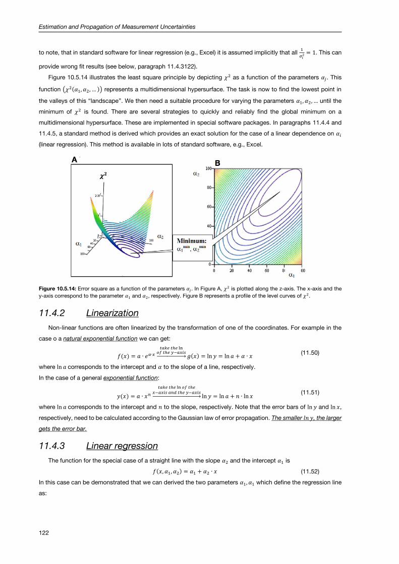
Estimation and Propagation of Measurement Uncertainties
122
to note, that in standard software for linear regression (e.g., Excel) it is assumed implicitly that all 1
𝜎𝑖2 = 1. This can
provide wrong fit results (see below, paragraph 11.4.3122).
Figure 10.5.14 illustrates the least square principle by depicting 𝜒2 as a function of the parameters 𝛼𝑗. This
function (𝜒2(𝛼1, 𝛼2, … )) represents a multidimensional hypersurface. The task is now to find the lowest point in
the valleys of this “landscape”. We then need a suitable procedure for varying the parameters 𝛼1, 𝛼2, … until the
minimum of 𝜒2 is found. There are several strategies to quickly and reliably find the global minimum on a
multidimensional hypersurface. These are implemented in special software packages. In paragraphs 11.4.4 and
11.4.5, a standard method is derived which provides an exact solution for the case of a linear dependence on 𝛼𝑖
(linear regression). This method is available in lots of standard software, e.g., Excel.
Figure 10.5.14: Error square as a function of the parameters 𝛼𝑗. In Figure A, 𝜒2 is plotted along the z-axis. The x-axis and the
y-axis correspond to the parameter 𝛼1 and 𝛼2, respectively. Figure B represents a profile of the level curves of 𝜒2.
11.4.2 Linearization
Non-linear functions are often linearized by the transformation of one of the coordinates. For example in the
case o a natural exponential function we can get:
𝑓(𝑥) = 𝑎 ∙ 𝑒𝛼∙𝑥
𝑡𝑎𝑘𝑒 𝑡ℎ𝑒 ln𝑜𝑓 𝑡ℎ𝑒 𝑦−𝑎𝑥𝑖𝑠→ 𝑔(𝑥) = ln 𝑦 = ln 𝑎 + 𝛼 ∙ 𝑥
(11.50)
where ln 𝑎 corresponds to the intercept and 𝛼 to the slope of a line, respectively.
In the case of a general exponential function:
𝑦(𝑥) = 𝑎 ∙ 𝑥𝑛
𝑡𝑎𝑘𝑒 𝑡ℎ𝑒 ln 𝑜𝑓 𝑡ℎ𝑒𝑥−𝑎𝑥𝑖𝑠 𝑎𝑛𝑑 𝑡ℎ𝑒 𝑦−𝑎𝑥𝑖𝑠→ ln 𝑦 = ln 𝑎 + 𝑛 ∙ ln 𝑥
(11.51)
where ln 𝑎 corresponds to the intercept and 𝑛 to the slope, respectively. Note that the error bars of ln 𝑦 and ln 𝑥,
respectively, need to be calculated according to the Gaussian law of error propagation. The smaller 𝑙𝑛 𝑦, the larger
gets the error bar.
11.4.3 Linear regression
The function for the special case of a straight line with the slope 𝛼2 and the intercept 𝛼1 is
𝑓(𝑥, 𝛼1, 𝛼2) = 𝛼1 + 𝛼2 ∙ 𝑥 (11.52)
In this case can be demonstrated that we can derived the two parameters 𝛼1, 𝛼1 which define the regression line
as:

Estimation and Propagation of Measurement Uncertainties
123
𝛼1 =𝑆𝑦 ∙ 𝑆𝑥2 − 𝑆𝑥𝑦 ∙ 𝑆𝑥
∆ (11.53)
𝛼2 =𝑆𝑥𝑦 ∙ 𝑆 − 𝑆𝑦 ∙ 𝑆𝑥
∆ (11.54)
with
𝑆 ≡∑ 1
𝜎𝑖2
𝑁
𝑖=1
(11.55)
𝑆𝑥 ≡∑ 𝑥𝑖
𝜎𝑖2
𝑁
𝑖=1
(11.56)
𝑆𝑦 ≡∑ 𝑦𝑖
𝜎𝑖2
𝑁
𝑖=1
(11.57)
𝑆𝑥2 ≡∑ 𝑥𝑖2
𝜎𝑖2
𝑁
𝑖=1
(11.58)
𝑆𝑥𝑦 ≡∑ 𝑥𝑖 ∙ 𝑦𝑖
𝜎𝑖2
𝑁
𝑖=1
(11.59)
∆= 𝑆 ∙ 𝑆𝑥2 − 𝑆𝑥 ∙ 𝑆𝑥 (11.60)
Excel and other softwares provide automatic calculations of the linear regression of a straight line. In these
softwares, the measuring values 𝑥𝑖 , 𝑦𝑖 etc. are not automatically weighted with 𝜎𝑖2, meaning with the variances of
𝑦𝑖. Therefore, the regression should be directly performed with the help of equations (11.53) and (11.54).
11.4.4 Estimation of the errors of the regression parameters
The influence of the error ∆𝑦𝑖 on the errors ∆𝛼1 and ∆𝛼2 can be determined with the help of the law of error
propagation (see paragraph 11.3.2)
∆𝛼𝑘2 =∑(
𝜕𝛼𝑘𝜕𝑦𝑖
)2
∙ ∆𝑦𝑖2
𝑛
𝑖=1
(11.61)
Using the equations (11.53) to (11.60) we can derive (see Appendix 11.5.4)
∆𝛼12 =
𝑆𝑥2
∆ (11.62)
∆𝛼22 =
𝑆
∆ (11.63)
Note that the evaluation of a fit (goodness of fit 𝜒2) and the comparison of different models is actually very
complex and demands some experience. Equations (11.62) and (11.63), respectively, give only a rough indication.
11.4.5 Important example
Here we consider the law of gravitation
𝑡 = √2 ∙ 𝐻
𝑔 (11.64)
where 𝐻, 𝑡 and 𝑔 denote the falling height, the falling time and the acceleration of gravity, respectively. The aim of
this example is to prove this law and to determine the gravitational acceleration. For this purpose, a set of
measured falling times 𝑡𝑗,𝑖 is collected for different falling heights 𝐻𝑗. The falling times are averaged according to
𝑡�̅� =1
𝑛𝑗∑ 𝑡𝑗,𝑖𝑛𝑗𝑖=1 (analogously to equation (11.3)) and the corresponding standard deviation 𝜎𝑡𝑗 can be calculated
(see equation (11.6)). Also the falling height is measured several times and is registered with the mean value 𝐻𝑗̅̅ ̅

Estimation and Propagation of Measurement Uncertainties
124
and the corresponding 𝜎ℎ𝑗. Linearization by double logarithmic plotting (according to (11.50)) yields a straight line
with the slope 𝛼2 = 1/2
log (𝑡
𝑠) = log((
2 ∙ 𝐻
𝑔)
12) = −
1
2∙ log (
𝑔
𝑚 𝑠2⁄) +
1
2∙ log (
2 ∙ 𝐻
𝑚) (11.65)
where log (𝑡
𝑠) corresponds to the y-axis, −
1
2∙ log (
𝑔
𝑚 𝑠2⁄) to the intercept 𝛼1,
1
2 to the slope 𝛼2 and log (
2∙𝐻
𝑚) to the 𝑥-
axis, like in
𝑦𝑖 = 𝛼1 + 𝛼2 ∙ 𝑥𝑖 (11.66)
Note that the numbers need to be dimensionless in their logarithm, since the logarithm of a unit does not make
physically sense. Therefore, each value is divided by its own dimension, e.g., 𝑡 is divided by 𝑠, 𝐻 by 𝑚 and 𝑔 by
𝑚
𝑠2, respectively. However, it is important to take care that the dimensions are consistent with the physical quantity.
This means that it is not allowed to mix up t/min, H/cm and g/(km/h2). The measuring data and the corresponding
evaluation are summarized in Table 10.5.2.
Before plotting the data in a graph (Figure 10.5.15), it is important to deal with the measuring error in order to
deduce the error bars. First, the errors in the direction of the abscissa are considered. For this it is assumed, that
the height is determined with an accuracy of ∆𝐻 = ±0.5𝑚. The 𝑥-axis plots log (2 ∙ 𝐻) and the corresponding error
is calculated according to the Gaussian error propagation
∆ log𝐻 = (𝜕 log(2 ∙ 𝐻)
𝜕𝐻) ∙ ∆𝐻 = 2 ∙
∆𝐻
𝐻 (11.67)
Determination of the errors in the direction of the ordinate (y-axis): Table 10.5.1 shows the data for 20 individual
measurements at a certain falling height. The mean value obtained by averaging is 𝑡̅ = 5.53 𝑠 and the
corresponding statistical error of an individual measurement 𝜎𝑡 = 0.278 𝑠 (see paragraph 11.2). Compared to this,
Table 10.5.2 shows the falling times for different falling heights and the falling time for a certain falling height was
obtained by averaging only three individual measurements, in order to limit the number of measurements.
Table 10.5.2: Data and their evaluation on the experiment about the law of gravitation.

Estimation and Propagation of Measurement Uncertainties
125
Figure 10.5.15: Double logarithmic plot of the data given in Table 10.5.2.
Thus, for the 20 measurements in Table 10.5.1 one obtains a mean deviation of the mean value of 𝜎𝑡̅,20 =𝜎
√20 and
analogously, for the falling times in Table 10.5.2 𝜎𝑡̅,3 =𝜎
√3= 0.15. Since log(t) is plotted on the y-axis, the error
bars in this direction is given by
∆ log 𝑡 = (𝜕 log(𝑡)
𝜕𝑡) ∙ 𝜎𝑡̅,3 =
𝜎𝑡̅,3𝑡
(11.68)
Beside the logarithmic conversion of the measuring data, Table 10.5.2 also gives calculated the length of the error
bars.
11.5 Appendixes
11.5.1 Function of several independent variables
In general, the 𝑁 measuring parameters 𝑥𝑘 and their respective errors are independent of each other.
On the basis of a measuring series, the measuring value is determined 𝑛 times (index 𝑖) and from this the
mean value 𝑥𝑘̅̅ ̅ and the corresponding standard deviation 𝜎𝑘 can be determined by
𝑥𝑘̅̅ ̅ =1
𝑛∙∑𝑥𝑖,𝑘
𝑛
𝑖=1
(11.69)
𝜎𝑘 = √1
𝑛 − 1∙∑(𝑥𝑖,𝑘 − 𝑥𝑘̅̅ ̅)
2𝑛
𝑖=1
(11.70)
From the 𝑖th measurement, one obtains the result 𝑓𝑖,𝑘 = 𝑓(𝑥𝑖,1, 𝑥𝑖,2, … ). In order to obtain the most reliable
result, one may calculate arithmetic mean of the individual results 𝑓̅ = 𝑓𝑖,𝑘(𝑥𝑖,1, 𝑥𝑖,2, … )̅̅ ̅̅ ̅̅ ̅̅ ̅̅ ̅̅ ̅̅ ̅̅ ̅̅ ̅̅ according to Equation
(11.69):
𝑓̅ =1
𝑛∙∑𝑓𝑖,𝑘
𝑛
𝑖=1
(11.71)
Alternatively, one can first calculate the arithmetic mean of the individual arguments 𝑥𝑘̅̅ ̅ from the same
Equation (11.69) and then calculate the result function:
𝑓̿ = 𝑓𝑖,𝑘(𝑥1̅̅ ̅, 𝑥2̅̅ ̅, … , 𝑥𝑁̅̅̅̅ ) (11.72)

Estimation and Propagation of Measurement Uncertainties
126
In order to compare 𝑓 ̅and 𝑓,̿ we consider the deviation of each individual measurement fi from the mean
value 𝑓 ̿by writing fi as Taylor expansion around 𝑓:̿
𝑓𝑖,𝑘 = 𝑓(𝑥1̅̅ ̅, 𝑥2̅̅ ̅, … , 𝑥𝑁̅̅̅̅ ) +∑(𝜕𝑓
𝜕𝑥𝑘)
𝑁
𝑘=1
∙ ∆𝑥𝑖,𝑘 +⋯ (11.73)
where the first term 𝑓(𝑥1̅̅ ̅, 𝑥2̅̅ ̅, … , 𝑥𝑁̅̅̅̅ ) = 𝑓 ̿while the following terms correspond to the deviation from 𝑓.̿ The
mean value 𝑓 ̅is now calculated by inserting Equation (11.71) into (11.72):
𝑓̅ =1
𝑛∙∑𝑓̿ +
1
𝑛
𝑛
𝑖−1
∙∑∑(𝜕𝑓
𝜕𝑥𝑘)
𝑁
𝑘=1
𝑛
𝑖=1
∙ ∆𝑥𝑖,𝑘 + 𝑞𝑢𝑎𝑑𝑟𝑎𝑡𝑖𝑐 𝑡𝑒𝑟𝑚𝑠 𝑒𝑡𝑐. (11.74)
Here, the first term equals 1
𝑛∙ ∑ 𝑓̿ =𝑛
𝑖−1 𝑓.̿ The second term 1
𝑛∙ ∑ ∑ (
𝜕𝑓
𝜕𝑥𝑘)𝑁
𝑘=1𝑛𝑖=1 ∙ ∆𝑥𝑖,𝑘 is zero, since reversing
the order of summation reveals ∑ (𝜕𝑓
𝜕𝑥𝑘)𝑁
𝑘=1 ∑ ∆𝑥𝑖,𝑘𝑛𝑖=1 with ∑ ∆𝑥𝑖,𝑘
𝑛𝑖=1 = 0. Consequently, as we already
showed for a single variable, mean values 𝑓(𝑥𝑖,1, 𝑥𝑖,2, 𝑥𝑖,3…)̅̅ ̅̅ ̅̅ ̅̅ ̅̅ ̅̅ ̅̅ ̅̅ ̅̅ ̅̅ ̅̅ and 𝑓̿ = (𝑥1̅̅ ̅, 𝑥2̅̅ ̅, … , 𝑥𝑁̅̅̅̅ ) coincide.
11.5.2 Standard deviation as a function of the variance
Here we derive the variance 𝜎𝑓2 (or its square root, the standard deviation 𝜎𝑓) of the result function 𝑓(𝑥)
𝜎𝑓2 ≈
1
𝑛 − 1∑(𝑓𝑖 − 𝑓)̅2 =
1
𝑛 − 1
𝑛
𝑖=1
∑ (∑(𝜕𝑓
𝜕𝑥𝑘)
𝑁
𝑘=1
∆𝑥𝑖,𝑘)
2𝑛
𝑖=1 (11.75)
where
(∑(𝜕𝑓
𝜕𝑥𝑘)
𝑁
𝑘=1
∆𝑥𝑖,𝑘)
2
== ∑(𝜕𝑓
𝜕𝑥𝑘)2
∆𝑥𝑖,𝑘2
𝑁
𝑘=1
+ ∑ (𝜕𝑓
𝜕𝑥𝑘) ∙ (
𝜕𝑓
𝜕𝑥𝑖)
𝑁
𝑘,𝑙=1𝑙≠𝑚
∆𝑥𝑖,𝑘 ∙ ∆𝑥𝑖,𝑙 (11.76)
Inverting the sigma signs reveals
𝜎𝑓2 = ∑(
𝜕𝑓
𝜕𝑥𝑘)2𝑁
𝑘=1
1
𝑛 − 1∙∑∆𝑥𝑖,𝑘
2
𝑛
𝑖=1
+1
𝑛 − 1∙ ∑ (
𝜕𝑓
𝜕𝑥𝑘) ∙ (
𝜕𝑓
𝜕𝑥𝑖)
𝑁
𝑘,𝑙=1𝑙≠𝑚
∙∑∆𝑥𝑖,𝑘 ∙ ∆𝑥𝑖,𝑙
𝑛
𝑖=1
(11.77)
and finally this yields the Gaussian law of error propagation
𝜎𝑓2 ≈
1
𝑛 − 1∑(𝑓𝑖 − 𝑓)̅2 =
1
𝑛 − 1
𝑛
𝑖=1
∑ (∑(𝜕𝑓
𝜕𝑥𝑘)
𝑁
𝑘=1
∆𝑥𝑖,𝑘)
2𝑛
𝑖=1 (11.78)
or analogously
𝜎𝑓 = √(𝜕𝑓
𝜕𝑥1)2
∙ 𝜎12 + (
𝜕𝑓
𝜕𝑥2)2
∙ 𝜎22 +⋯ (11.79)
11.5.3 The principle of “maximum likelihood”
We assume that the values 𝑦𝑖 are normally distributed according to a Gaussian distribution. Having the right
parameter set 𝛼1…𝛼𝑗 …𝛼𝑛, the expectation value of 𝑦 is given by 𝑓( 𝑥1 , 𝑥,…2 𝛼1, 𝛼2, … ). In this case, the probability
𝑤𝑖 to obtain the value 𝑦𝑖 in an individual measurement would be
𝑤𝑖 =1
𝜎𝑖√
1
2 ∙ 𝜋∙ 𝑒
−(𝑦𝑖−𝑓( 𝑥𝑖,
1 𝑥𝑖…,𝛼1,𝛼2…𝛼𝑝2 ))
2
2∙𝜎𝑖2
(11.80)

Estimation and Propagation of Measurement Uncertainties
127
The total probability 𝑊 for the whole set of measurements is then given by the product of the probabilities of each
individual measurement
𝑊 = 𝑤1 ∙ 𝑤2 ∙ 𝑤3 ∙ … =
=1
𝜎1 ∙ 𝜎2 ∙ …(√
1
2 ∙ 𝜋)
𝑁
∙ 𝑒−(𝑦1−𝑓( 𝑥1,
1 𝑥1…,𝛼1,𝛼2…𝛼𝑝2 ))
2
2∙𝜎12
∙ 𝑒−(𝑦2−𝑓( 𝑥2,
1 𝑥2…,𝛼1,𝛼2…𝛼𝑝2 ))
2
2∙𝜎22
∙ …
(11.81)
where
𝑒−(𝑦1−𝑓( 𝑥1,
1 𝑥1…,𝛼1,𝛼2…𝛼𝑝2 ))
2
2∙𝜎12
∙ 𝑒−(𝑦2−𝑓( 𝑥2,
1 𝑥2…,𝛼1,𝛼2…𝛼𝑝2 ))
2
2∙𝜎22
== 𝑒−∑
(𝑦𝑖−𝑓( 𝑥2,1 𝑥2…,𝛼1,𝛼2…𝛼𝑝
2 ))2
2∙𝜎𝑖2
𝑁𝑖=1
(11.82)
If the parameter set is correct, then the probability 𝑊 becomes maximal. This occurs if the negative exponent (≡
1
2∙ 𝜒2) in equation (11.82) is minimal. Thus equation (11.49) (𝜒2) needs to be minimal.
11.5.4 Deriving the errors of the regression parameters
The influence of the error ∆𝑦𝑖 on the errors ∆𝛼1 and ∆𝛼2 can be determined with the help of the law of error
propagation (see paragraph 11.3.2)
Equations (11.62) can be derived by substituting equation (11.53) in (11.61), obtaining:
∆𝛼12 =∑(
𝜕 (𝑆𝑦 ∙ 𝑆𝑥2 − 𝑆𝑥𝑦 ∙ 𝑆𝑥
∆)
𝜕𝑦𝑖)
2
∙ ∆𝑦𝑖2 ==∑(
𝜕𝑆𝑦𝜕𝑦𝑖
∙ 𝑆𝑥2 −𝜕𝑆𝑥𝑦𝜕𝑦𝑖
∙ 𝑆𝑥
∆)
2
∙ ∆𝑦𝑖2
𝑛
𝑖=1
𝑛
𝑖=1
(11.83)
where 𝜕𝑆𝑦
𝜕𝑦𝑖=
1
𝜎𝑖2,
𝜕𝑆𝑥𝑦
𝜕𝑦𝑖=
𝑥𝑖
𝜎𝑖2 and ∆𝑦𝑖
2 = 𝜎𝑖2. Squaring out the bracket yields
∆𝛼12 =∑(
𝑆𝑥2 ∙1𝜎𝑖2 − 𝑆𝑥 ∙
𝑥𝑖𝜎𝑖2
∆)
2
∙ 𝜎𝑖2 =
𝑛
𝑖=1
=1
∆2∑(𝑆𝑥2
2 ∙𝜎𝑖2
𝜎𝑖4 − 2 ∙ 𝑆𝑥 ∙ 𝑆𝑥2 ∙
𝑥𝑖 ∙ 𝜎𝑖2
𝜎𝑖4 + 𝑆𝑥
2 ∙𝑥𝑖2 ∙ 𝜎𝑖
2
𝜎𝑖4 )
𝑛
𝑖=1
(11.84)
and further using ∑1
𝜎𝑖2
𝑛𝑖=1 = 𝑆, ∑
𝑥𝑖
𝜎𝑖2
𝑛𝑖=1 = 𝑆𝑥 and ∑
𝑥𝑖2
𝜎𝑖2
𝑛𝑖=1 = 𝑆𝑥
2
∆𝛼12 =
1
∆2∙ (𝑆𝑥2
2 ∙∑1
𝜎𝑖2
𝑛
𝑖=1
− 2 ∙ 𝑆𝑥 ∙ 𝑆𝑥2 ∙∑𝑥𝑖
𝜎𝑖2
𝑛
𝑖=1
+ 𝑆𝑥2 ∙∑
𝑥𝑖2
𝜎𝑖2
𝑛
𝑖=1
) == 𝑆𝑥2 ∙𝑆 ∙ 𝑆𝑥2 − 𝑆𝑥 ∙ 𝑆𝑥
∆2 (11.85)
Using equation (11.60) 𝑆 ∙ 𝑆𝑥2 − 𝑆𝑥 ∙ 𝑆𝑥 = ∆ finally yields (11.62). Equation (11.63) can be analogously derived.