labor market segmentation and the distribution of income
TRANSCRIPT
DEPARTMENT OF ECONOMICS WORKING PAPER SERIES
Labor Market Segmentation and the Distribution of Income: New Evidence from Internal Census Bureau Data
Ellis Scharfenaker Markus P. A. Schneider
Working Paper No: 2019-08
August 2019
University of Utah
Department of Economics 260 Central Campus Drive
Gardner Commons, Rm. 1400 Salt Lake City, UT 84112
Tel: (801) 581-7481 http://www.econ.utah.edu
Labor Market Segmentation and the Distribution of Income: New Evidence from
Internal Census Bureau Data*
Ellis Scharfenaker Department of Economics, University of Utah
Markus P. A. Schneider Department of Economics, University of Denver
Abstract
In this paper, we present new findings that validate earlier literature on the apparent segmentation of the US earnings distribution. Previous contributions posited that the observed distribution of earnings combined two or three distinct signals and was thus appropriately modeled as a finite mixture of distributions. Furthermore, each component in the mixture appeared to have distinct distributional features hinting at qualitatively distinct generating mechanisms behind each component, providing strong evidence for some form of labor market segmentation. This paper presents new findings that support these earlier conclusions using internal CPS ASEC data spanning a much longer study period from 1974 to 2016. The restricted-access internal data is not subject to the same level of top-coding as the public-use data that earlier contributions to the literature were based on. The evolution of the mixture components provides new insights about changes in the earnings distribution including earnings inequality. In addition, we correlate component membership with worker type to provide a tacit link to various theoretical explanations for labor market segmentation, while solving the problem of assigning observations to labor market segments a priori.
Keywords: Inequality, Income Distribution, Mixture Model
JEL Classification: C16, D32, J01
*The research in this paper was conducted while all authors were Special Sworn Status researchers of the U.S. Census Bureau at the Rocky Mountain Research Data Center at the University of Colorado. Any opinions and conclusions expressed herein are those of the authors and do not necessarily represent the views of the U.S. Census Bureau. All results have been reviewed to ensure that no confidential information is disclosed.
Introduction
Schneider (2013) proposed that a finite mixture distributional model may be used to
reconcile economists traditional intuitions about the shape of the distribution of income
with physicists’ more recent findings that incomes appear roughly exponentially distributed
up to relatively high levels. Using CPS data, the author showed that based on a variety of
fit criteria a finite mixture model consisting of an exponential component and a log-normal
component fits the data better than either the exponential or the log-normal distributions
alone, and better than most alternatives. Schneider (2015) critically revisits the physics
literature on the distribution of income and verifies the earlier finding using IRS tax data.
In fact, the finite mixture model performs on par with the commonly used generalized beta of
the 2nd kind (GB2) distribution used by Feng, Burkhauser, and Butler (2006), Burkhauser,
Feng, Jenkins, and Larrymore (2008), Jenkins (2009).
In this paper, we show that the results presented in Schneider (2013) are robust by using
internal Census data that is top-coded at a much higher reporting threshold than the public-
use data used in the original paper. Specifically, we pick up the research question whether the
US income distribution can be characterized by a mixture of frequency distributions that has
finite components and that is stable with respect to the number and type of components. In
addition to using data with a much higher top-code limit, we provide fits over a much longer
period and provide stronger evidence for the long-run stability of the functional features of
our model.
The changes in the parameter estimates provide novel insights about the evolution of
the income distribution from 1975 to the present. Both Schneider (2013) and Schneider
(2015) asserted that the components of the mixture model have more intuitive economic in-
terpretations than more complicated distributions like the GB2. In what follows, we provide
a cursory overview of the literature, briefly outline the intuition behind the specific two-
component mixture model, and discuss a variety of unresolved issues. We then present the
3

results for the exponential-log normal mixture based on internal Census data for earnings
from 1974 to 2016.
Our project adds to a growing recent literature using publicly available IRS and CPS data
to estimate finite mixture models with distinctive components, yielding remarkably accurate
fits of the observed frequencies (Dragulescu and Yakovenko, 2001, Yakovenko and Silva, 2005,
Yakovenko, 2007, Shaikh, Papanikolaou, and Wiener, 2014, Schneider, 2015). These models
e↵ectively identify the presence of at least two distinct and formally persistent “signals”
in the U.S. distribution of income: a power-law distribution for high-income individuals
(Parker and Fenwick, 1983, Fichtenbaum and Shahidi, 1988, Bishop, Chiou, and Fromby,
1994, Champernowne and Cowell, 1998, Yakovenko, 2007, Philip Armour, 2014) and an
exponential. Schneider (2013) and Schneider (2015) further suggest the possibility of an
additional log-normal component in the mixture. Since all the work in this literature relies
on publicly available data, a verification using the restricted-access data available through
the US Census Bureau constitutes an important contribution, not least of all because top-
coding and binning procedures for the public-use data periodically change over time. While
the work cited above takes great care to adjust appropriately, there is no substitute for the
richer restricted-use CPS ASEC data covering a longer study period.
Background
Dagum (1977) contrasted two approaches in inquiry into the observed frequency distri-
butions of income, defined by whether those distributions are taken to represent a tractable
expression of the processes conditioning individual incomes or simply fit a shape to the
observed distribution. Much recent work e↵ectively rejects the proposition that there is
a tractable connection between the best fitting functional form of a distribution fit to the
data and the underlying generating mechanism. That is, the observed shape of the distribu-
tion of income is not held to reveal insights about the workings of labor markets. Current
4
approaches instead emphasize the identification of the best-fitting general shapes for the
observed distributions, paying little attention to what this may imply for economic theory.
Explanatory parsimony is downplayed in favor of goodness of fit. The limit of this approach
is a non-parametric fitting of the observed distribution, but in application it is more com-
mon to use a very flexible parametric distribution like the GB2. A good representation of
researchers working in this second paradigm is given by Feng et al. (2006), Burkhauser et al.
(2008), Jenkins (2009). While these more flexible models tend to provide a good fit to the
empirical data, they provide little in the way of a theoretical explanation of the generative
processes and a priori exclude the possibility of multiple distinct labor markets each with
their own statistical signature. Before revisiting why this appears to be the preferred ap-
proach at present, we want to outline the alternative, which is the focus of this paper, has a
long pedigree in the history of economic thought.
The alternative approach seeks to understand well-fitting distributions as expressions of
the underlying market processes generating income. Work following this approach seeks to
establish analytical linkages between the distribution(s) it identifies and plausible economic
behavior or functioning. Parsimony and the ability to inform economic theorization are the
central principles of analysis. This approach mirrors the methodological approach physicists
take to studying distributional data. Its history parallels the history of advances in Statistical
Mechanics, where the Principle of Maximum Entropy allowed formal consideration of the
relationship between the micro-level “laws of motion” governing the interactions between
individual particles and the macroscopic properties of large collections of particles, including
the distributions of certain quantities across particles.
The earliest contributions in this tradition date back to the turn of the last century. Vil-
fredo Pareto devoted considerable e↵ort to the construction of income and wealth frequency
distributions for several countries, leading to his discovery at the very top of income ranges
of the kind of “fat tail” distributions that today bear his name. Pareto postulated this com-
5
mon distribution constituted a fundamental “social law” in capitalist economies. This work
was furthered by Gibrat (1931), who considered that the growth of enterprises followed geo-
metric processes, which he associated with log-normal distributions for their size. Analogous
multiplicative “laws of motion” were soon put forward for income-generating processes and
linked to specific predictions concerning individual distributions of income. Kalecki (1945)
pointed out that such a process (e.g. if experience and education increase worker skill in a
multiplicative, rather than additive, fashion) could lead both to log-normal and to power-law
distributions (see also Sutton (1997)).
Problems for this approach arose by the middle of the 20th century, when Lydall (1959)
showed that the observed distribution of income did not appear to be log-normal. More
recent contributions grounded on this methodological approach have consistently uncovered
evidence for power-law behavior among high incomes and rejected the proposition that in-
comes were log-normally distributed, but they failed to settle on a convincing fit for the bulk
of the distribution (Dagum, 1977, Bordley, McDonald, and Mantrala, 1997, Champernowne
and Cowell, 1998). The shift towards simple shape-fitting was at least partially motivated
by the perceived failure to conclusively identify how the bulk of incomes are distributed.
One casual justification for shape-fitting was a collective resignation that the observed dis-
tribution of income pooled the outcomes from many di↵erent process. Given a su�ciently
large number of diverse processes, any distributional shape could arise and identification of
a best-fitting distribution would be a futile endeavor.
Concurrently, economists developed ideas about labor market segmentation that on the
one hand would indeed suggest that the observed distribution of income pools observations
from di↵erent processes, but also that the number of processes is finite and limited in number.
Furthermore, one can extrapolate that each process has distinct features, so that under the
assumption that markets are entropy maximizing process (Foley, 1994), each labor market
segment should be assumed to produce a distinct stable distributional signature. However,
6

this line of reasoning was not pursued until Schneider (2013).
Partially, this may have been because one version of labor market segmentation, the
“dual labor market” theory of Reich, Gordon, and Edwards (1973), pursued a more narra-
tive approach for characterizing the qualitative di↵erences between labor market processes.
Other explanations for segmentation provided formal models, but none of them explored
the implications for the stable shape of the observed distribution (see Weitzman, 1989, for
example). This reflects in part a disciplinary limit in how economists tend to think about
equilibrium. Economists instinct is to think of prices as uniquely determined and thus any
distribution of prices to only reflect some underlying distribution of determinants (e.g. innate
ability, human capital, etc.). It is exactly in this regard that (Foley, 1994) o↵ers the novel
deviation by showing what happens when the restriction that agents only make maximizing
exchanges is relaxed to allow all Pareto-improving exchanges. The result is that a statis-
tical equilibrium distribution of prices emerges that is the result of an entropy maximizing
process. The empirical implication is that if we can identify the distribution consistent with
this statistical equilibrium, it can help us characterize the specific features of the underlying
market process as the constraints in an entropy maximization program (MaxEnt).
This approach, however, also immediately implies some intellectual limitations. The
reverse implication of the this approach is that any process that is consistent with the iden-
tified constraints in the MaxEnt program is a possible explanation for the data. That is,
this approach allows us to demarcate between theories that have distinctly di↵erent distribu-
tional implications, but not between theories that have the same distributional implications.
For instance, after convincing themselves that incomes appeared exponentially distributed,
physicists have posited a conservation law for the total wage-bill while economists (who reject
this notion) might point to the mean-preserving growth or a “social scaling” mechanism (dos
Santos, 2017). Since all of these are consistent with the exponential arising as an entropy
maximizing distribution in statistical equilibrium, the observation of the exponential cannot
7
help di↵erentiate between these hypotheses. Only additional information that leads us to
favor the premises behind one position over the others could be used to demarcate between
them.
It may seem like a basic point, but it has direct bearing on the results we are presenting
in this paper and how we interpret them. Specifically, we show empirical evidence for the
number and plausible type of distributional components, but do not endeavor to discrimi-
nate which plausible explanation for labor market segmentation may be ruled out by these
findings. More work needs to be done to answer this broader question with any satisfaction.
Su�ce it to say for the purposes of this paper that there several explanations for segmenta-
tion have been put forth and we remain agnostic about which one we favor. More detailed
investigation may reveal that not all can be reconciled equally well with our findings, but
confounding the issue is that they may also not all be mutually exclusive.
For concreteness, the main competing theories we have in mind include the narrative
proposed by Reich et al. (1973) that describes a primary labor market bifurcated into subor-
dinate and independent jobs and a secondary labor market comprised of unstable low wage
jobs. Weitzman (1989) proposed a formal model based on wage stickyness and uncertainty
about labor demand that he suggests is consistent with Reich et al. (1973).1 The thrust of
Weitzman (1989)’s model is that two strategies employer strategies evolve and may exist in
what he calls sticky wage stochastic competitive equilibrium (p. 127): some employers o↵er
higher wages to maintain a stable work force, which works because they also commit to
higher per employee capital intensity in production, while other employers insure against
economic uncertainty through a low-wage / low-capital intensity strategy in order to “thrust
the burden of unstable business on a casual work force.” (p. 123) Perhaps most importantly,
Weitzman (1989) argues that the emergent pattern of segmentation is likely to be largely in-
1Weitzman (1989) concedes that his model is su�ciently abstract to be consistent with a number ofdi↵erent explanations.
8

dependent of any initial skill distribution, because any arbitrary sorting into one or the other
kind of job can result in an employee being labeled in a way that proves self-reenforcing.
In particular, this leaves open a mechanism for characteristics that are unrelated to
actual productivity di↵erences to become determinant of a worker’s employment trajectory.
Economic stratification (see Jr., Hamilton, and Stewart, 2015), for example, seems like an
easily reconcilable feature of the kind of segmentation described by Weitzman (1989), where
implicit bias, previous wages, di↵erential educational opportunities, etc. all serve as the
kind of self-fulfilling labeling system that sorts female and minority workers into lower-
wage, precarious employment. A somewhat di↵erent argument for a similarly racialized
segmentation is given by Temin (2017), who suggests that the US is regressing towards a
dual economy as characterized by the Lewis model originally proposed to explain disparate
sectors in developing countries. There are clear di↵erences in this conception from the one
o↵ered by Weitzman (1989)’s model,2 though it is unclear to us whether these di↵erences
might not be reconcilable.
Dickens and Lang (1993) make the point that any of the diverse appeals to segmenta-
tion are a counter to standard human capital theory as an explanation for wage dispersion.
For instance, they di↵er from search-theoretic explanations for wage dispersion, like Mont-
gomery (1991), that tend to either assume or conclude that there is a strict correlation (if
not outright equality) between individual worker’s pay and they productivity, taken as ex-
ogenously determined. This still applies when one reads the authoritative Acemoglu and
Autor (2011), who posit wage dispersion in a perfect labor market as a consequence of skill
di↵erentials. The key point for the present work is that we look for a statistical signature
of segmentation that goes beyond simply the level of wage dispersion. Our interpretation of
2Not least, the Lewis model posits that the marginal product of labor in the less developed sector is zero(or approximately zero), whereas the individual worker’s marginal product is actually irrelevant in Weitzman(1989).
9
labor market segmentation is that it implies a finite set of qualitatively di↵erent signals in
the overall observed distribution of income from labor, which is a more concretely testable
claim than simply o↵ering di↵erent explanations for an observed growing dispersion between
the incomes of di↵erent workers.
It appears, however, that this was not fully recognized by the advocates for labor market
segmentation either. Osterman (1975) recognizes the identification problem resulting form
sorting worker-observations a priori and Dickens and Lang (1993) directly address the senti-
ment that labor market segmentation is an untestable proposition. In fact, Schneider (2013)
attributes the recent stagnation of this line of work to the failure to consider finite mixture
models, which o↵er a systematic approach for testing the evidence in favor of segmentation
without the pre-sorting problem discussed by Osterman (1975). The core idea is that since
di↵erent labor market segments operate in a qualitatively di↵erent ways, thus generating
di↵erent stationary distributions, comparing the fit of di↵erent specifications of a finite mix-
ture model3 can reveal both the number and type of segments evident in the data. This
paper, however, does not present the comprehensive investigation with respect to number
and type of segments supported by the data, but more modestly looks at the robustness of
the results presented by Schneider (2013) using a richer dataset over a longer period.
Recent work by Lubrano and Ndoye (2016), Anderson, Farcomeni, Pittau, and Zelli
(2016), Anderson, Pittau, Zelli, and Thomas (2018) has applied finite mixtures models to
labor market data. While this research has clearly made important contributions to the un-
derlying statistical methodology of finite mixture models it has remained pragmatic about
the particular distributional form used, often employing the log normal distribution due to
its convenient statistical properties. The ambition of this paper is apply the same statistical
methodology of finite mixture models while also giving serious consideration to the distinct
3What amounts to a spectral analysis of the earnings distribution.
10
characteristics of each component. This approach leads us to consider the statistical dis-
similarity of each labor market segment. Our results thus extend the work of Lubrano and
Ndoye (2016), Anderson et al. (2016, 2018) to the use finite mixture models with diverse
components.
Specific Model
Both the narrative theory of Reich et al. (1973) or the model by Weitzman (1989) posit a
labor market segment that matches workers to positions that fundamentally do not rely on
the individual attributes of a given worker. These may be positions described as “low-skill”
(or better, highly routinized) where workers filling them can be treated as homogeneous
not because they are, but because their attributes and skills matter very little to getting
the job done, thus a relatively constant wage should prevail. As Weitzman (1989) makes
clear, the key feature of this segment is that workers absorb all uncertainty and thus pay
fluctuations from one period to the next. As we will argue, this combination of relatively
constant wage and high earnings churn as the result of precarious employment (or at least
hours) is quite consistent with an exponential distribution of earnings. By contrast, another
labor market (itself perhaps bifurcated) does match employers and employees based on the
individual worker’s work history. Here, the multiplicative combination of past experience
(and pay) should give rise to either a log-normal or power-law distribution of wages.
We further posit that looking at earnings, we are necessarily conflating the wage and
the number of hours worked. However, workers in the latter segment are much more likely
to hold full-time positions with an expectation of 40 hours of work per week. Variations in
hours is likely to be much less than variation in wages and thus the distribution of incomes
should be expected to largely reflect the distribution of wages. On the other hand, workers
who fill positions that simply require a body are more likely to occupy jobs with less than
full-time hours and have highly variable hours across the year. (Seasonal hires in retail,
11
services, or agriculture for example.) For this segment, variation in incomes is more likely
come from the hours worked than the wages paid. We speculate that it is this latter labor
market segment that is captured by the apparent exponential distribution of low to moderate
incomes discovered by physicists in the early 2000s (see Dragulescu and Yakovenko, 2001,
Yakovenko and Silva, 2005, Yakovenko, 2007). Rather than a conservation law of money
(as the physicists in question postulated), we posit that the exponential reflects a relatively
constant overall demand for basic labor with a lot of dynamic churn across sectors in a given
year as to where exactly basic labor is required.
A simple preliminary test to see if this line of reasoning might prove salient is to see if
the specific components in our mixture model are correlated with the appropriate worker
type (full-time or part-time). If it is indeed the case that part-time workers dominate the
exponential component of the mixture, it also provides a link to the framing provided the
literature on stratification. That literature has shown that who performs basic labor in
the economy – defined by low wages, no benefits, variable hours below full-time – is highly
gendered and racialized. Contrary to the popular belief that part-time jobs paying the
minimum wage are filled predominantly by high schoolers getting their first work experience,
they are much more likely to employ men and women of color past high-school age. If the
correlation between worker type holds, it will warrant further investigation whether the
expected correlation with worker race and gender also holds, and this will reveal exactly
who occupies each of the labor market segments that we identify. It also gives credence to
the role of “labeling” mechanisms postulated by Weitzman (1989).
While these considerations present valuable directions for future research, they are beyond
the scope of the present paper, which simply shows how an exponential-log normal mixture
fits the observed distribution of income, that this fits is stable across a relatively long period,
and then tests the correlation between worker type and mixture component to show that
indeed part-time workers dominate the exponential component of the mixture.
12
Methodology
We follow the innovations by Borzadaran and Behdani (2009), Scharfenaker and Semie-
niuk (2016), Scharfenaker and Foley (2017), Shaikh et al. (2014), dos Santos (2017) that
draw on Information Theory and Statistical Mechanics to develop economically meaningful
accounts of these inferred distributions. In relation to individual income, the observation
of frequencies that are consistently well-described by a specific functional distribution al-
lows the use of the Principle of Maximum Entropy to infer the aggregate, mathematical
forms taken by the processes shaping those distributions. Those will be given by the ag-
gregate constraints defining the statistical ensemble over which the observed distributions
are entropy maximizing, as argued by E. T. Jaynes. In many instances, it is possible to
advance plausible economic processes capable of generating such constraints. For example,
exponential distributions may provide evidence that wage incomes embody the competitive
“social scaling” of unobservable measures of physical productivity and bargaining power over
money wages, as argued in dos Santos (2017); log-normal distributions may in turn reflect
a stochastic evolution of income that is on average proportional to previous income. It is
thus likely that distinct “signals” in the observed distribution of income reveal the existence
of formally distinct modes of income appropriation in line with the theory of labor market
segmentation.
A nuance to this approach is to recognize that while it may be the case that the under-
lying market processes are entropy maximizing (as argued by Foley, 1994, for instance), the
Principle of Maximum Entropy put forth by E. T. Jaynes suggests that the solution to a pro-
gram that maximizes Shannon’s entropy is relevant even if the process is not strictly entropy
maximizing. Even in this case, the MaxEnt solution presents the most probably description
– barring the incorporation of explicit information of the actual process. Put di↵erently, the
MaxEnt solution imposes the least restrictive prior when the underlying when it is not known
whether the underlying process is entropy maximizing or not. The twist to this underlying
13

the present investigation is that we assume each mixture component (corresponding to a
distinct labor market segment) is best modeled as a maximum entropy distribution, while
we do not make any assumptions whether the number of components is somehow entropy
maximizing.
Data
Like Schneider (2013), we use CPS person-level earnings data from the ASEC (March
Supplement). The variable WSAL-VAL combines wage and salary income across multiple
jobs, but excludes self-employment income as well as non-labor income. Because of avail-
ability issues, Schneider (2013) was limited to a series of public-use data from 1996 to 2007.
Furthermore, the public-use data was subject to relatively low top-code limits that were
accounted for in the estimation by using the top-code limit as a censoring limit and using
the top-code flag as a count of censored observations.
The analysis in this paper uses restricted-access CPS ASEC data gathered from the
Federal Statistical Research Data Center (RDC). With this restricted-access data we can ex-
amine the WSAL-VAL variable from 1974 to 2016 which is also subject to a much higher (less
restrictive) top-code limit. We still treat top-coded observations as censored and make the
appropriate adjustment in our maximum likelihood estimations, but our robustness checks
indicate that this has only a minor (and not economically meaningful) impact on the actual
estimates.
Top-coding is potentially a major limitation when using the publicly available data.
The variable used in our study, WSAL-VAL, is the sum of two variables recorded during
data collection: ERN-VAL and WS-VAL, or earnings from primary and secondary jobs
respectively. According to the CPS documentation, these variables are top-coded before
they are added to create WSAL-VAL. If one or the other, or both, earnings components
are top-coded, it is di�cult to model the uncertainty that is being introduced through the
14
truncation procedure. Schneider (2013) dealt with this by dealing with all observations
that contained a top-coded value as censored and using the top-code as the censoring limit.
Since we are using restricted access data, this is not an issue in the work presented in this
paper beyond the censoring of the data above the internal recording limit already mentioned.
For more information on the topcoding issue, see Larrimore, Burkhauser, Feng, and Zayatz
(2008).
There are several procedural changes to the CPS ASEC dataset during the study win-
dow,4 two of which deserve explicit mention. First, data collection changed from paper-and-
pencil to computer assisted in 1993. Along with this change, certain recording limits on
income variables were adjusted; most relevantly for us, earnings up to $999,999 were now
recorded. There were also expected adjustments to implement the 1990 Census population
controls in 1992 and further adjustments in 1994 to update the sample design. All together,
the changes made in this period appear to produce a notable “jump” in some estimates
presented in this paper (similar jumps are seen in Larrimore et al., 2008, Schneider, 2013,
2015, for example). There was also a significant redesign in 2014 of the CPS ASEC, but it
does not appear to produce the kind of discontinuity that resulted from the changes in 1993.
Second, there is a large change in sample size in 2002. From 1975 to 2001, the CPS ASEC
contained 60,000 to 87,000 raw observations; from 2002 to 2008, over 100,000 observations
were recorded before it slowly declined back down to 87,000 by 2017. However, the March
supplement weights used to match the CPS ASEC sample to the larger CPS and last Census
seem to successfully adjust for variations in sample sizes such that estimates do not seem to
fluctuate with sample size in any notable way because the sample weights, MARSUPWT,
su�ciently ensure that samples remain representative of the population.5
4https://www.census.gov/topics/income-poverty/income/guidance/cps-methodology-changes.
html
5We suspect that Larrimore et al. (2008) may understate the impact of topcoding by focusing on thenumber of observations subject to topcoding, not their population weight. Since the weights are in principle
15
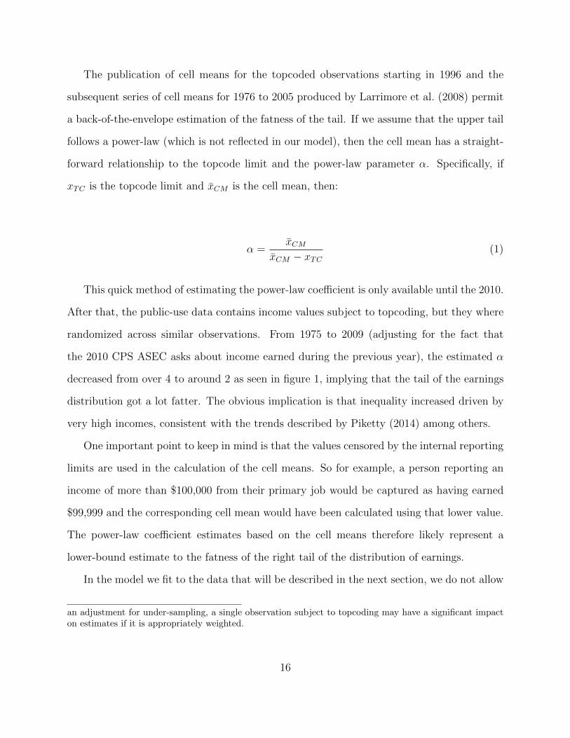
The publication of cell means for the topcoded observations starting in 1996 and the
subsequent series of cell means for 1976 to 2005 produced by Larrimore et al. (2008) permit
a back-of-the-envelope estimation of the fatness of the tail. If we assume that the upper tail
follows a power-law (which is not reflected in our model), then the cell mean has a straight-
forward relationship to the topcode limit and the power-law parameter ↵. Specifically, if
x
TC
is the topcode limit and x
CM
is the cell mean, then:
↵ =x
CM
x
CM
� x
TC
(1)
This quick method of estimating the power-law coe�cient is only available until the 2010.
After that, the public-use data contains income values subject to topcoding, but they where
randomized across similar observations. From 1975 to 2009 (adjusting for the fact that
the 2010 CPS ASEC asks about income earned during the previous year), the estimated ↵
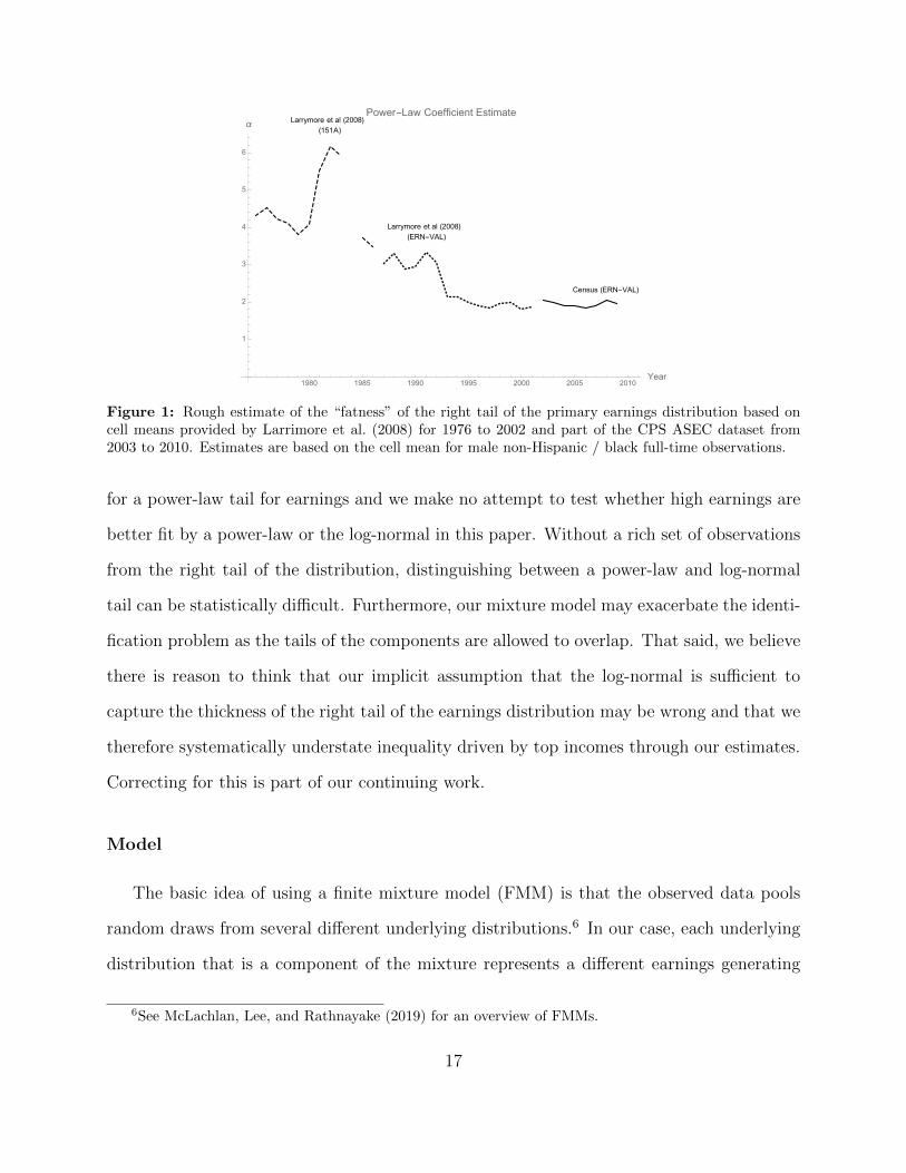
decreased from over 4 to around 2 as seen in figure 1, implying that the tail of the earnings
distribution got a lot fatter. The obvious implication is that inequality increased driven by
very high incomes, consistent with the trends described by Piketty (2014) among others.
One important point to keep in mind is that the values censored by the internal reporting
limits are used in the calculation of the cell means. So for example, a person reporting an
income of more than $100,000 from their primary job would be captured as having earned
$99,999 and the corresponding cell mean would have been calculated using that lower value.
The power-law coe�cient estimates based on the cell means therefore likely represent a
lower-bound estimate to the fatness of the right tail of the distribution of earnings.
In the model we fit to the data that will be described in the next section, we do not allow
an adjustment for under-sampling, a single observation subject to topcoding may have a significant impacton estimates if it is appropriately weighted.
16
Larrymore et al (2008)(151A)
Larrymore et al (2008)(ERN-VAL)
Census (ERN-VAL)
1980 1985 1990 1995 2000 2005 2010Year
1
2
3
4
5
6
αPower-Law Coefficient Estimate
Figure 1: Rough estimate of the “fatness” of the right tail of the primary earnings distribution based oncell means provided by Larrimore et al. (2008) for 1976 to 2002 and part of the CPS ASEC dataset from2003 to 2010. Estimates are based on the cell mean for male non-Hispanic / black full-time observations.
for a power-law tail for earnings and we make no attempt to test whether high earnings are
better fit by a power-law or the log-normal in this paper. Without a rich set of observations
from the right tail of the distribution, distinguishing between a power-law and log-normal
tail can be statistically di�cult. Furthermore, our mixture model may exacerbate the identi-
fication problem as the tails of the components are allowed to overlap. That said, we believe
there is reason to think that our implicit assumption that the log-normal is su�cient to
capture the thickness of the right tail of the earnings distribution may be wrong and that we
therefore systematically understate inequality driven by top incomes through our estimates.
Correcting for this is part of our continuing work.
Model
The basic idea of using a finite mixture model (FMM) is that the observed data pools
random draws from several di↵erent underlying distributions.6 In our case, each underlying
distribution that is a component of the mixture represents a di↵erent earnings generating
6See McLachlan, Lee, and Rathnayake (2019) for an overview of FMMs.
17
mechanism, where the di↵erence could be one simply of scale or a more fundamental di↵er-
ence. By varying the component types being considered in addition to the number of mixture
components, we can allow for heterogeneity both in terms of the number of segments as well
as their underlying generating mechanisms.
Since we are looking at fundamentally one-dimensional data (income), such mixture
models are relatively straightforward to estimate using Maximum Likelihood Estimation
(MLE) and this is typical in the literature.7 In general we specify the total distribution
of income as X where p[x] is a probability density function of X such that p[x] � 0 andRp[x]dx = 1. Assuming the distribution of income is generated by a K-component finite-
mixture distribution, this impliesX is a linear combination ofK component density functions
each with a respective weight �k
(s.t.P
K
k=1 �K
= 1), and each parameterized by a vector ✓k
.
The probability density assigned to making the observation x
i
is therefore given by:
p[xi
|✓1, . . . , ✓k] =KX
k=1
�
k
p
k
[xi
|✓k
] (2)
This model defines a likelihood for the N observed incomes {xi
}N
conditional on the
K-component mixture model:
p[{xi
}N
|✓1, . . . , ✓k] =NY
i=1
KX
k=1
�
k
p
k
[xi
|✓k
] (3)
The discovery that a finite mixture model provides a thorough and stable statistical de-
scription of the distribution of income shows that heterogeneity inherent in labor markets
and allow us to obtain good estimates of the evolution of the parameters for each distribu-
7Lubrano and Ndoye (2016) details some of the benefits from Bayesian methods as well.
18
tional form we identify as well as of their relative weights in the overall distribution. The
result is that each labor market segment is endogenously determined by the data itself.
The specific model we fit in this paper is the two-component exponential-log normal
mixture model first applied to publicly available CPS data in Schneider (2013). This model
takes the following four parameter form:
p[xi
|↵, µ, �,�] = �Exp[xi
|�] + (1� �) lgN[xi
|µ, �] (4)
The use of finite mixture models thus allows for overlapping distributions without ad
hoc sorting of workers into each proposed segment (see Osterman, 1975) with hard cut-o↵
incomes as is common in existing literature (see Dragulescu and Yakovenko, 2000).
To test what type of worker falls into each component of the mixture, we can estimate
the component weight, �, as conditional on worker type. For the initial analysis presented
here, we use an administrative dummy variable that codes all workers reporting that they
typically work less than 35 hours per week as “part-time” (PT) and all workers that typically
work 35 hours or more as “full-time” (FT). The conditional expression of � is simply:
� = �0 + �1 FT (5)
The estimated propensity for a PT worker to be in the exponential component of the
mixture is therefore given by �0 and that of a FT worker by �0 + �1. If PT workers in-
deed dominate the exponential component of the mixture, then we expect a negative and
statistically significant estimate of �1.
19
Model Results
For the sake of brevity, we do not present formal fit comparisons to other models in this
paper and instead concentrate on interpreting what the fit of the proposed mixture model
given by equation (4) tells us. However, based on Schwarz’s Bayesian Information Criteria
(BIC), the mixture model provides an overwhelmingly better fit of the earnings data than
either the exponential or log-normal components alone. It also provides a better fit than
the Gamma distribution, which only very modestly improves on the fit of the exponential.
The GB2 distribution does provide a better fit of the data, which we largely attribute to its
greater ability to fit a power-law tail.8 A systematic evaluation of the best model specification
is part of our ongoing project.
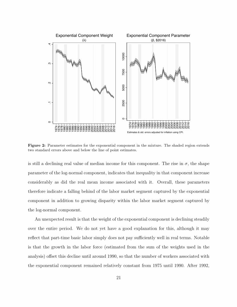
Figure 2 and 3 plots the evolution of the estimated model parameters (ML estimates are
detailed in Appendix A). The parameter � is the inverse of the exponential scale parameter
and is the mean of the exponential component of the mixture model. Both µ and � are
adjusted for inflation using the CPI.
We now note a few trends in the parameter evolutions and provide some interpretation.
The scale parameters of both components of the mixture, when adjusted for inflation, decline
over the period 1975 to 2017. This is consistent with stagnant median incomes and slow
growth in mean incomes. What our model adds is that mean and median incomes captured
in the exponential component declined significantly since 1975 (see the top right panel in
fig. 2). If, as we speculate, the exponential component is dominated by workers earning the
minimum wage or near it, then this makes sense as the minimum wage persistently eroded
in real value from its peak in 1968.
The decline in µ (bottom left panel) is less precipitous and more steady, consistent with
the log-normal component reflecting somewhat less precarious employment. The implication
8Schneider (2013) using the public-use data and a di↵erent fit criteria found that the GB2 and theexponential / lognormal mixture provided comparable fits of the data.
20
0.1
.2.3
.4
1974
1976
1978
1980
1982
1984
1986
1988
1990
1992
1994
1996
1998
2000
2002
2004
2006
2008
2010
2012
2014
2016
(λ)Exponential Component Weight
025
0050
0075
0010
000
1974
1976
1978
1980
1982
1984
1986
1988
1990
1992
1994
1996
1998
2000
2002
2004
2006
2008
2010
2012
2014
2016
Estimates & std. errors adjusted for inflation using CPI.
(β, $2016)Exponential Component Parameter
Figure 2: Parameter estimates for the exponential component in the mixture. The shaded region extendstwo standard errors above and below the line of point estimates.
is still a declining real value of median income for this component. The rise in �, the shape
parameter of the log-normal component, indicates that inequality in that component increase
considerably as did the real mean income associated with it. Overall, these parameters
therefore indicate a falling behind of the labor market segment captured by the exponential
component in addition to growing disparity within the labor market segment captured by
the log-normal component.
An unexpected result is that the weight of the exponential component is declining steadily
over the entire period. We do not yet have a good explanation for this, although it may
reflect that part-time basic labor simply does not pay su�ciently well in real terms. Notable
is that the growth in the labor force (estimated from the sum of the weights used in the
analysis) o↵set this decline until around 1990, so that the number of workers associated with
the exponential component remained relatively constant from 1975 until 1990. After 1992,
21

1010
.511
1974
1976
1978
1980
1982
1984
1986
1988
1990
1992
1994
1996
1998
2000
2002
2004
2006
2008
2010
2012
2014
2016
Estimates adjusted for inflation using CPI.
(μ, ln$2016)Log-Normal Scale Parameter
.5.6
.7.8
1974
1976
1978
1980
1982
1984
1986
1988
1990
1992
1994
1996
1998
2000
2002
2004
2006
2008
2010
2012
2014
2016
(σ)Log-Normal Shape Parameter
Figure 3: Parameter estimates for the log-normal component in the mixture. The shaded region extendstwo standard errors above and below the line of point estimates.
the number of workers in the exponential component declined from around 30 million to 20
million because labor force growth slowed. (Note that the trend in � shown in the top left
panel does not show a notable change around 1990-1992.)
1980 1990 2000 2010
-0.02
-0.01
0.00
0.01
0.02
0.03
λ cycle
Figure 4: Cyclical variation in HP filtered � against NBER business cycles.
22

We want to also note that according to Weitzman (1989)’s interpretation of his model,
we should expect the share of more contingent and precarious workers to rise at the on-
set of a recession as employers switch to production strategies that shifts risk to workers.
Since we speculate that such workers are represented by the exponential component of the
mixture, this provides a testable hypothesis about the cyclical movement of the exponential
component’s weight (�). While there are not enough business cycle downturns in our study
window to form any firm conclusions, the prediction does appear consistent with the cyclical
movement of �: each of the downturns in our data are associated with a temporary increase
�.
For further clarity we compare the density evolution of the income distribution as cap-
tured by the model in Figure 10 for 1974 and 2016.
0 20000 40000 60000 80000 100000Earnings ($2016)
1974 2016
(1974 & 2016)Fitted Earnings Density Function (Mixture)
Figure 5: Fitted earnings densities for 1974 and 2016 illustrating the evolution of the distribution of incomesbased on the two-component mixture. The thin dashed lines show the components for 1974 (weighted by �)and the thin solid lines show the components for 2016.
23
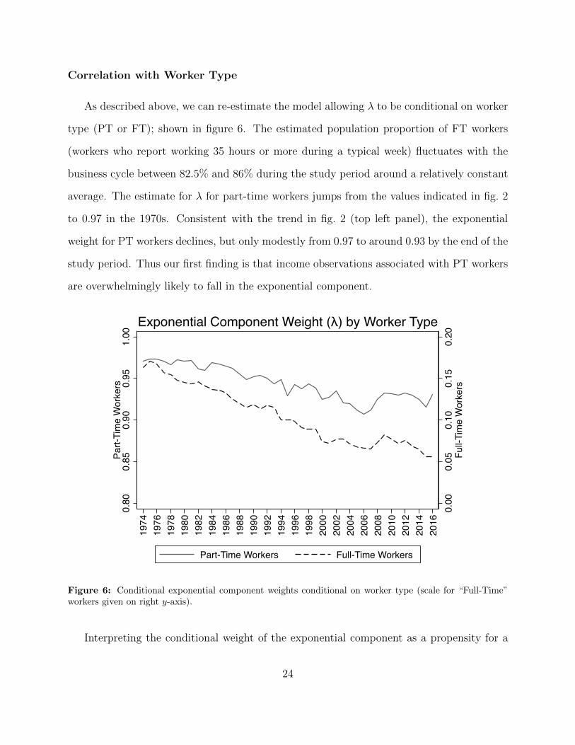
Correlation with Worker Type
As described above, we can re-estimate the model allowing � to be conditional on worker
type (PT or FT); shown in figure 6. The estimated population proportion of FT workers
(workers who report working 35 hours or more during a typical week) fluctuates with the
business cycle between 82.5% and 86% during the study period around a relatively constant
average. The estimate for � for part-time workers jumps from the values indicated in fig. 2
to 0.97 in the 1970s. Consistent with the trend in fig. 2 (top left panel), the exponential
weight for PT workers declines, but only modestly from 0.97 to around 0.93 by the end of the
study period. Thus our first finding is that income observations associated with PT workers
are overwhelmingly likely to fall in the exponential component.
0.00
0.05
0.10
0.15
0.20
Full-
Tim
e W
orke
rs
0.80
0.85
0.90
0.95
1.00
Part-
Tim
e W
orke
rs
1974
1976
1978
1980
1982
1984
1986
1988
1990
1992
1994
1996
1998
2000
2002
2004
2006
2008
2010
2012
2014
2016
Part-Time Workers Full-Time Workers
Exponential Component Weight (λ) by Worker Type
Figure 6: Conditional exponential component weights conditional on worker type (scale for “Full-Time”workers given on right y-axis).
Interpreting the conditional weight of the exponential component as a propensity for a
24
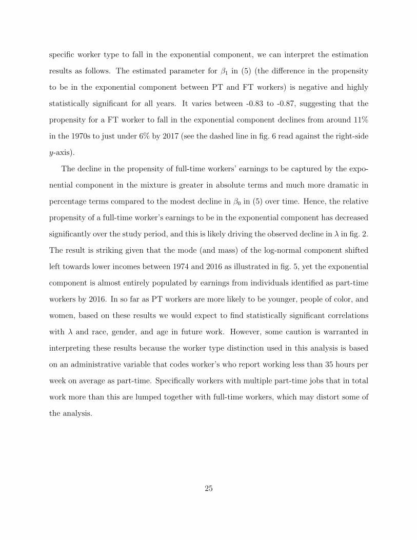
specific worker type to fall in the exponential component, we can interpret the estimation
results as follows. The estimated parameter for �1 in (5) (the di↵erence in the propensity
to be in the exponential component between PT and FT workers) is negative and highly
statistically significant for all years. It varies between -0.83 to -0.87, suggesting that the
propensity for a FT worker to fall in the exponential component declines from around 11%
in the 1970s to just under 6% by 2017 (see the dashed line in fig. 6 read against the right-side
y-axis).
The decline in the propensity of full-time workers’ earnings to be captured by the expo-
nential component in the mixture is greater in absolute terms and much more dramatic in
percentage terms compared to the modest decline in �0 in (5) over time. Hence, the relative
propensity of a full-time worker’s earnings to be in the exponential component has decreased
significantly over the study period, and this is likely driving the observed decline in � in fig. 2.
The result is striking given that the mode (and mass) of the log-normal component shifted
left towards lower incomes between 1974 and 2016 as illustrated in fig. 5, yet the exponential
component is almost entirely populated by earnings from individuals identified as part-time
workers by 2016. In so far as PT workers are more likely to be younger, people of color, and
women, based on these results we would expect to find statistically significant correlations
with � and race, gender, and age in future work. However, some caution is warranted in
interpreting these results because the worker type distinction used in this analysis is based
on an administrative variable that codes worker’s who report working less than 35 hours per
week on average as part-time. Specifically workers with multiple part-time jobs that in total
work more than this are lumped together with full-time workers, which may distort some of
the analysis.
25
Measures of Inequality
Economists study the distribution of income in order to provide a sound basis for public
policy that aims to reduce harmful social and economic e↵ects of inequality. Both earlier
empirical work on the dual-labor market (Reich et al., 1973, Osterman, 1975, Weitzman,
1989) and recent work on the dual structure of the US economy (Temin, 2017) suggests
that single summary statistics of income inequality are insu�cient for understanding the
relationship between policy and programs, and their distributional consequences.
The benefit of a segmented labor market approach is not only the ability to identify
distinct labor market segments, but also to identify a more detailed measure of inequality in
economy by examining the within and between inequalities of each component. Following
Dagum (1997) and Anderson et al. (2018) with a population of size N with total income Y
partitioned into K (possibly overlapping) subpopulations where nk
represents the population
in the k
th group such thatP
k
n
k
= N and f
k
is the distribution function of kth group then,
letting the population share and income share in group k be p
k
= nkN
and s
k
= µk
µ
, where
µ
k
is the average income in group k, and with G
k
representing the weighted Gini of the k
th
group, the total Gini coe�cient can be decomposed into three components:
G = G
w
+G
b
+G
t
(6)
Where
G
w
=KX
k=1
p
2k
s
k
G
k
(7)
measures the contribution of within subpopulation inequality to the total Gini,
G
b
=1
µ
KX
k=2
k�1X
j=i
p
k
p
j
|µk
� µ
j
| (8)
26
measures the contribution of between subpopulation inequality and
G
t
=2
µ
KX
k=2
k�1X
j=i
p
k
p
j
Z 1
0
f
k
[y]
Z 1
y
f
j
[x](x� y)dxdy (9)
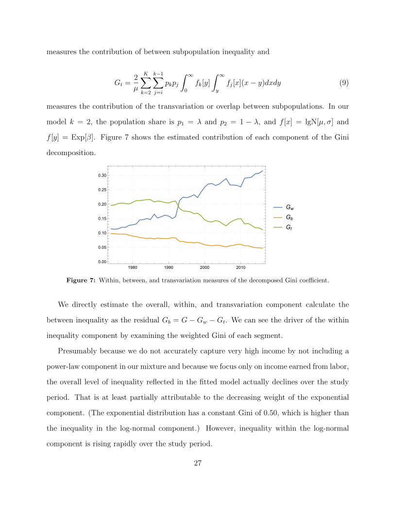
measures the contribution of the transvariation or overlap between subpopulations. In our
model k = 2, the population share is p1 = � and p2 = 1 � �, and f [x] = lgN[µ, �] and
f [y] = Exp[�]. Figure 7 shows the estimated contribution of each component of the Gini
decomposition.
1980 1990 2000 20100.00
0.05
0.10
0.15
0.20
0.25
0.30
GwGbGt
Figure 7: Within, between, and transvariation measures of the decomposed Gini coe�cient.
We directly estimate the overall, within, and transvariation component calculate the
between inequality as the residual Gb
= G � G
w
� G
t
. We can see the driver of the within
inequality component by examining the weighted Gini of each segment.
Presumably because we do not accurately capture very high income by not including a
power-law component in our mixture and because we focus only on income earned from labor,
the overall level of inequality reflected in the fitted model actually declines over the study
period. That is at least partially attributable to the decreasing weight of the exponential
component. (The exponential distribution has a constant Gini of 0.50, which is higher than
the inequality in the log-normal component.) However, inequality within the log-normal
component is rising rapidly over the study period.
27
1980 1990 2000 20100.0
0.1
0.2
0.3
0.4
0.5
Gini
GGlgNGexp
Figure 8: Total inequality and within segment inequality measured by the Gini coe�cient.
Because all three components of GINI are non-negative and 0 G
t
G, we can follow
Anderson et al. (2018) and define a segmentation index which measures of the degree to
which constituent segments do not overlap:
SI = 1� G
t
G
=2µ
PK
k=2
Pk�1j=1 pkpj
R10
f
k
[y]R1y
f
j
[x](x� y)dxdy
1� 1µ
R1�1(1� F [x])2 dx
(10)
1980 1990 2000 20100.50
0.55
0.60
0.65
0.70
0.75
SI
Figure 9: Estimated segmentation index.
Because the transvariation measure in Figure 7 is declining we see that the segmentation
index is rising, implying that the upper segment represented by the log-normal component is
28
being pulled further to the right. This picture appears consistent with the findings of Piketty
(2014) who shows the income share of the top earners as increasing dramatically after 1990.
Conclusion
The search for the best functional fit for the observed distribution of income has often
ignored fundamental di↵erences in income generating mechanisms across labor markets. The
concept of a homogeneous labor market naturally leads to explanations of the variation in
income as arising from individual characteristics. This conceptualization of a labor market
process operating uniformly on all individuals leads to the modeling of the income distri-
bution in a single encompassing functional form. The theory of labor market segmentation
identifies qualitative di↵erences between various labor market processes and has a natural
interpretation in finite mixture models. In this paper we have demonstrated the usefulness
of finite mixture modeling for analyzing a heterogeneous labor market incorporating the
complexities of the various functional forms that arise from theoretical considerations.
Using restricted-access Census data, our initial results indicate that the exponential-log
normal mixture model provides a stable fit to the distribution of income for the period 1975-
2017. Furthermore, we find that the parameter evolution clarifies details of the changing
distribution of income over this period. Most notably, incomes captured by the log-normal
component become more dispersed. The exponential component’s relative contribution to
the mixture appears to shrink while the mean and median income of that component de-
creases considerably.
Most significantly, we show that the exponential component is associated with part-time
workers, supporting our prior that it represents the labor market for workers supplying basic
labor and facing highly variable hours of work.
Decomposing the Gini coe�cient, we also demonstrate that labor markets are becoming
more segmented as indicated by the rising segmentation index. This segmentation appears
29
to be worsening considerable since 1990 in line with the rising income share of top income
earners.
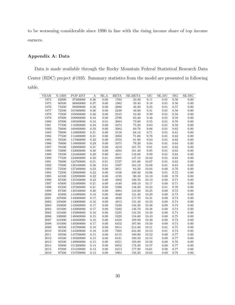
Appendix A: Data
Data is made available through the Rocky Mountain Federal Statistical Research Data
Center (RDC) project #1935. Summary statistics from the model are presented in following
table.
YEAR N OBS POP EST A SE A BETA SE BETA MU SE MU SIG SE SIG1974 62000 97400000 0.36 0.00 1763 33.40 9.11 0.01 0.56 0.001975 60500 96800000 0.37 0.00 1982 39.30 9.18 0.01 0.56 0.001976 73500 99400000 0.36 0.00 2088 40.30 9.25 0.01 0.57 0.001977 72500 101900000 0.36 0.00 2249 46.60 9.31 0.01 0.58 0.001978 73500 105000000 0.36 0.00 2545 54.00 9.39 0.01 0.58 0.001979 87000 108800000 0.34 0.00 2796 63.40 9.46 0.01 0.59 0.001980 87000 109500000 0.34 0.01 3084 73.00 9.55 0.01 0.59 0.001981 77500 110200000 0.34 0.00 3274 75.20 9.63 0.01 0.59 0.001982 76000 109400000 0.32 0.00 3082 69.70 9.66 0.01 0.62 0.001983 76000 110800000 0.31 0.00 3158 68.10 9.71 0.01 0.61 0.001984 77500 114400000 0.31 0.00 3303 71.60 9.76 0.01 0.62 0.001985 76500 117000000 0.32 0.00 3703 81.90 9.83 0.01 0.62 0.001986 76000 118800000 0.29 0.00 3475 76.20 9.84 0.01 0.64 0.001987 76500 120800000 0.31 0.00 4219 101.70 9.91 0.01 0.62 0.001988 72000 123000000 0.30 0.00 4294 101.40 9.95 0.01 0.63 0.001989 78500 124400000 0.29 0.00 4611 116.80 9.99 0.01 0.64 0.001990 77500 124600000 0.30 0.01 5095 147.10 10.02 0.01 0.63 0.001991 76000 124700000 0.31 0.01 5727 191.60 10.07 0.01 0.63 0.001992 75000 126100000 0.30 0.01 5507 164.10 10.09 0.01 0.64 0.001993 72500 127400000 0.23 0.00 3851 84.20 10.04 0.00 0.70 0.001994 72500 129900000 0.22 0.00 4100 100.30 10.06 0.01 0.72 0.001995 64500 132900000 0.22 0.00 4195 96.50 10.10 0.00 0.70 0.001996 65500 135500000 0.22 0.00 4462 106.50 10.13 0.00 0.71 0.001997 65000 135400000 0.21 0.00 4540 109.10 10.17 0.00 0.71 0.001998 65500 137200000 0.21 0.00 5396 148.20 10.24 0.01 0.70 0.001999 67500 140100000 0.20 0.00 4984 124.80 10.25 0.00 0.72 0.002000 65000 141000000 0.18 0.00 5049 131.40 10.29 0.00 0.73 0.002001 107000 143000000 0.17 0.00 4830 117.70 10.31 0.00 0.74 0.002002 105000 143000000 0.16 0.00 4913 121.40 10.33 0.00 0.74 0.002003 103000 142800000 0.17 0.00 5230 134.30 10.36 0.00 0.73 0.002004 101000 143900000 0.17 0.00 5292 136.70 10.38 0.00 0.74 0.002005 101000 145900000 0.16 0.00 5235 134.50 10.40 0.00 0.74 0.002006 100000 148000000 0.15 0.00 5220 134.80 10.43 0.00 0.75 0.002007 101000 149400000 0.16 0.00 6458 189.90 10.49 0.00 0.72 0.002008 101000 149300000 0.17 0.00 6452 187.80 10.50 0.00 0.74 0.002009 98500 145700000 0.18 0.00 6814 214.80 10.51 0.01 0.75 0.002010 95500 144300000 0.18 0.00 7205 244.20 10.53 0.01 0.74 0.002011 93500 145700000 0.15 0.00 6115 180.90 10.52 0.00 0.77 0.002012 94500 148300000 0.15 0.00 6181 180.50 10.54 0.00 0.77 0.002013 93500 149800000 0.15 0.00 6351 193.80 10.56 0.00 0.76 0.002014 93000 151200000 0.14 0.00 6052 178.30 10.57 0.00 0.77 0.002015 87000 154100000 0.13 0.00 6213 177.90 10.61 0.00 0.77 0.002016 87500 155700000 0.13 0.00 5964 156.20 10.64 0.00 0.78 0.00
30
����
����
����
����
����
����
����
����
����
0 20000 40000 60000 80000 100000 120000 140000
����
����
����
����
����
����
����
����
����
����
����
����
����
����
����
����
����
����
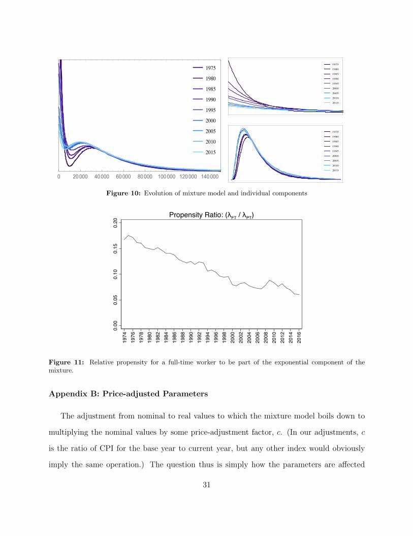
Figure 10: Evolution of mixture model and individual components
0.00
0.05
0.10
0.15
0.20
1974
1976
1978
1980
1982
1984
1986
1988
1990
1992
1994
1996
1998
2000
2002
2004
2006
2008
2010
2012
2014
2016
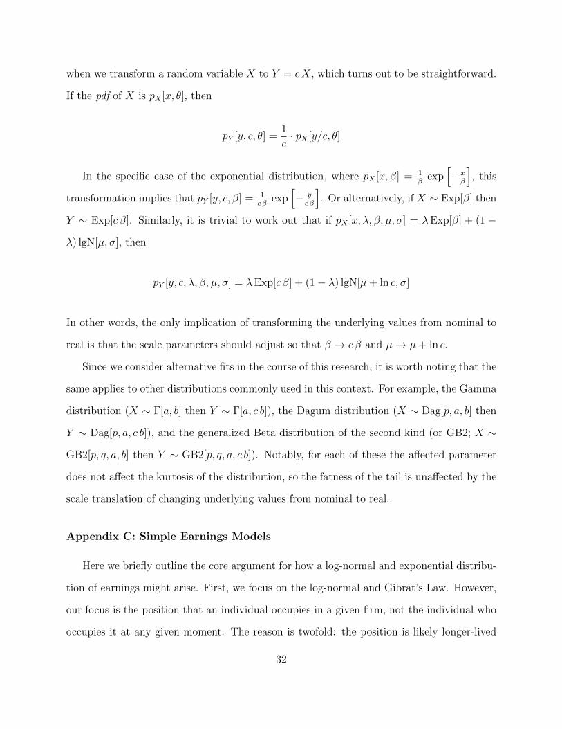
Propensity Ratio: (λFT / λPT)
Figure 11: Relative propensity for a full-time worker to be part of the exponential component of themixture.
Appendix B: Price-adjusted Parameters
The adjustment from nominal to real values to which the mixture model boils down to
multiplying the nominal values by some price-adjustment factor, c. (In our adjustments, c
is the ratio of CPI for the base year to current year, but any other index would obviously
imply the same operation.) The question thus is simply how the parameters are a↵ected
31
when we transform a random variable X to Y = cX, which turns out to be straightforward.
If the pdf of X is pX
[x, ✓], then
p
Y
[y, c, ✓] =1
c
· pX
[y/c, ✓]
In the specific case of the exponential distribution, where p
X
[x, �] = 1�
exph�x
�
i, this
transformation implies that pY
[y, c, �] = 1c�
exph� y
c�
i. Or alternatively, if X ⇠ Exp[�] then
Y ⇠ Exp[c �]. Similarly, it is trivial to work out that if pX
[x,�, �, µ, �] = �Exp[�] + (1 �
�) lgN[µ, �], then
p
Y
[y, c,�, �, µ, �] = �Exp[c �] + (1� �) lgN[µ+ ln c, �]
In other words, the only implication of transforming the underlying values from nominal to
real is that the scale parameters should adjust so that � ! c � and µ ! µ+ ln c.
Since we consider alternative fits in the course of this research, it is worth noting that the
same applies to other distributions commonly used in this context. For example, the Gamma
distribution (X ⇠ �[a, b] then Y ⇠ �[a, c b]), the Dagum distribution (X ⇠ Dag[p, a, b] then
Y ⇠ Dag[p, a, c b]), and the generalized Beta distribution of the second kind (or GB2; X ⇠
GB2[p, q, a, b] then Y ⇠ GB2[p, q, a, c b]). Notably, for each of these the a↵ected parameter
does not a↵ect the kurtosis of the distribution, so the fatness of the tail is una↵ected by the
scale translation of changing underlying values from nominal to real.
Appendix C: Simple Earnings Models
Here we briefly outline the core argument for how a log-normal and exponential distribu-
tion of earnings might arise. First, we focus on the log-normal and Gibrat’s Law. However,
our focus is the position that an individual occupies in a given firm, not the individual who
occupies it at any given moment. The reason is twofold: the position is likely longer-lived
32
than any individual’s tenure at the firm (possible longer than any individual’s lifetime) and
we would expect strong correlation of remuneration for any individual(s) occupying that po-
sition from one period to the next. (We are purposefully non-committal as to whether there
is substitutability between positions as there might be in a neoclassical setup or if positions
appear in fixed proportions within a given firm.)
The point is that a given firm requires a certain set of positions to be filled and pay
associated with each is determined by the role of that position within the firm’s production
process. Initially, that pay is y0. From one period to the next, the pay to each position
is adjusted and we let the adjustment be some random percentage increase, ✏t
, from the
original pay. So period 1 pay is:
y1 = (1� ✏
t
) y0
and after T periods, yT
=Q
T
t=1 (1� ✏
t
) y0. The heroic assumption on our part is that
each ✏
t
is i.i.d. with mean m and variance �
2< 1. To see how heroic this assumption is
consider everything that is being included in the stochastic raise: cost-of-living adjustments,
specific pay adjustments for hiring an over- or underqualified person to fill the position
(i.e. the individual characteristics of the individual filling the position and thus changes in
the individual filling the position), changes in technology that result in a revaluation of the
relative contribution of the position to production, etc. Lumping these things together and
considering them random while also postulating that across positions they are i.i.d. makes
✏
t
a very comprehensive catch-all.
Given that assumption and furthermore assuming that m is small (much closer to zero
than to unity; practically less than 0.1), we can make the usual simplification by taking the
log of the above expression and then approximating ln (1 + ✏
t
) ⇡ ✏
t
.
33
ln yT
=TX
t=1
t ln (1� ✏
t
) + ln y0 ⇡TX
t=1
✏
t
+ ln y0
Applying the Central Limit Theorem, we can make the case that ln yT
will be approxi-
mately normally distributed. Furthermore, the initial value y0 will play a vanishingly small
role in determining the mean of the distribution as long as T ·m >> y0. In other words, far
from the inception period, the distribution of pay associated with di↵erent positions is more
determined by the stochastic evolution over many periods than their original pay based
on their relative contribution to production. Here it is important, however, to remember
that the stochastic evolution itself included technological changes that rearrange the relative
value of di↵erent position within the production process. To put it concretely, a position that
started as a highly paid job might well end up towards the lower end of the pay spectrum
if technological change has made the particular skillset close to obsolete over the years. We
are treating that evolution as part of the “random” shocks ✏t
. The end result is that yT
is
asymptotically log-normally distributed and this distribution holds for a number of di↵erent
positions across the economy as long as the associated specific starting salaries associated
with them are small compared to the accumulated e↵ects of cost-of-living pay adjustments,
technological change, etc.
Maintaining a similar focus on positions at firms that are longer lived than individuals
(or anyway their tenure in a specific position), we now turn to the exponential distribution.
We posit that there is some work that can be done by any employee and e�cacy with which
it is done is the same across employees. The only thing that matters for these tasks is that
the work gets done, not by whom or their particular skill set. In very short time frames,
the total work of this nature is probably a fixed amount at the firm level. So maybe we can
imagine routinized service work that fundamentally amounts to little more than having an
employee behind the counter during open-for-business hours.
34
Formally, it may be very di�cult to assign remuneration to this type of work because it
has a discrete impact on firm operations. If it does not get done, none of the other productive
activity succeed and its marginal contribution is infinite; if it gets done, production succeeds
and any more of it leads to no more production so that it’s marginal contribution is zero.
Some firms may solve this problem by enticing or coercing existing employees in positions
not dedicated to such tasks to complete such them in addition to their direct responsibilities
essentially for free (or very low pay). Other firms, particularly in the service sector, may hire
part-time employees who are essentially interchangeable and with overall su�ciently flexible
schedules that these basic tasks can always be covered. If one employee is not available,
another gets their hours that week, for example.
In very short time frames, the total amount of time required for these tasks across em-
ployees is fixed and furthermore changes between short periods appear like a binary exchange
in hours between workers. Finally, if the workers filling these kinds of positions are paid ap-
proximately the same (which would almost certainly be the case within each establishment,
but is likely to even hold across establishments), then this all amounts to an argument how
an exponential distribution of earnings among these workers might arise.
Formally, the argument from physics that applies here is that the number of hours any two
employees (among many) supply is determined by their respective probabilities of agreeing
to work a certain number of hours, x1 and x2 respectively. We assume that the probability
functions are the same for each employee, so that the probability of them together working
x1 + x2 hours is f [x1] · f [x2]. On the other hand, the total amount of time required is
fixed, X, and thus the particular combination of x1 + x2 implies that the overall scheduling
arrangement must be such that X� (x1 + x2). If all scheduling arrangements are considered
equally likely, then the probability of such an overall scheduling arrangement must be equal
to the probability of x1 + x2. Thus, the probability distribution function we are looking for
has the property that:
35

f [x1] · f [x2] = h (x1 + x2)
The only function that will satisfy this equality is the exponential, thus suggesting that
the choice of hours across employees will have follow an exponential distribution. Further-
more, if all such employees are paid the same wage, then their earnings distribution will
also be exponential. The key to making this line of reasoning plausible is that the required
schedule fluctuations amongst employees happen at a much faster time scale than changes
in the aggregate hours of basic routine work across business. As we have presented it, we
envision schedule changes week-to-week and suspect that total hours required change no
faster than quarterly and maybe only annually. Thus the “churn” in schedules is 10 to 50
times faster than growth in the aggregate constraint.
References
Acemoglu, D., Autor, D., 2011. Skills, tasks and technologies: Implications for employmentand earnings. In: Handbook of labor economics. Vol. 4. Elsevier, pp. 1043–1171.
Anderson, G., Farcomeni, A., Pittau, M. G., Zelli, R., 2016. A new approach to measuringand studying the characteristics of class membership: Examining poverty, inequality andpolarization in urban china. Journal of Econometrics 191, 348–359.
Anderson, G., Pittau, M. G., Zelli, R., Thomas, J., 2018. Income inequality, cohesiveness andcommonality in the euro area: A semi-parametric boundary-free analysis. Econometrics6 (15).
Bishop, J., Chiou, J., Fromby, J., 1994. Truncation bias and the ordinal evaluation of incomeinequality. Journal of Business and Economic Statistics 12, 123–127.
Bordley, R. F., McDonald, J. B., Mantrala, A., 1997. Something new, something old: Para-metric models for the size of distribution of income. Journal of Income Distribution 6 (1),91–103.
Borzadaran, G., Behdani, Z., 2009. Maximum entropy and the entropy of mixing for incomedistributions. Journal of Income Distribution 18 (2), 179–186.
Burkhauser, R. V., Feng, S., Jenkins, S., Larrymore, J., 2008. Estimating trends in usincome inequality using the current population survey: The importance of controlling forcensoring. Journal of Economic Inequality 9 (3), 393–415.
36
Champernowne, D. G., Cowell, F. A., 1998. Economic Inequality and Income Distribution.Cambridge University Press, Cambridge.
Dagum, C., 1977. A new model of personal income distribution: Specification and estimation.Economie Appliquee 30, 413–426.
Dagum, C., 1997. A new approach to the decomposition of the gini income inequality ratio.Empirical Economics 22, 515–531.
Dickens, W. T., Lang, K., 1993. Labor market segmentation theory: reconsidering the evi-dence. In: Labor economics: Problems in analyzing labor markets. Springer, pp. 141–180.
dos Santos, P. L., Forthcoming 2017. The principle of social scaling. Complexity, Forthcom-ing.
Dragulescu, A., Yakovenko, V., 2000. Statistical mechanics of money. The European PhysicalJournal B - Condensed Matter and Complex Systems 17 (4), 723–729.
Dragulescu, A., Yakovenko, V. M., 2001. Evidence for the exponential distribution of incomein the usa. The European Physical Journal B 20, 585–589.
Feng, S., Burkhauser, R. V., Butler, J., 2006. Levels and long-term trneds in earnings inequal-ity: Overcoming current population survey censoring problems using the gb2 distribution.Journal of Business and Economic Statistics 24 (1), 57–62.
Fichtenbaum, R., Shahidi, H., 1988. Truncation bias and the measurement of income in-equality. Journal of Business and Economic Statistics 6, 335–337.
Foley, D. K., 1994. A statistical equilibrium theory of markets. Journal of Economic Theory62 (2), 321–345.
Gibrat, R., 1931. Les Inegalites Economiques. Librairie du Rucueil Sirey, Paris.
Jenkins, S. P., 2009. Distributionally-sensitive inequality indices and the gb2 income distri-bution. Review of Income and Wealth 55 (2), 392–298.
Jr., W. A. D., Hamilton, D., Stewart, J. B., 2015. A tour de force in understanding intergroupinequality: An introduction to stratification economics. Review of Black Political Economy42, 1–6.
Kalecki, M., 1945. On the Gibrat Distribution. Econometrica 13, 161–170.
Larrimore, J., Burkhauser, R. V., Feng, S., Zayatz, L., 2008. Consistent cell means fortopcoded incomes in the public use march cps (1976 - 2007). Journal of Economic andSocial Measurement 33 (2-3), 89–128.
37
Lubrano, M., Ndoye, A. A. J., 2016. Income inequality decomposition using a finite mixtureof log-normal distributions: A bayesian approach. Computational Statistics and DataAnalysis 100, 830–846.
Lydall, H. A., 1959. The Distribution of Employment Incomes. Econometrica 27, 110–115.
McLachlan, G. J., Lee, S. X., Rathnayake, S. I., 2019. Finite mixture models. Annual reviewof statistics and its application 6, 355–378.
Montgomery, J. D., 1991. Equilibrium wage dispersion and interindustry wage di↵erentials.The Quarterly Journal of Economics 106 (1), 163–179.
Osterman, P., 1975. An Empirical Study of Labor Market Segmentation. Industrial andLabor Relations 28, 508–523.
Parker, R. N., Fenwick, R., 1983. The pareto curve and its utility for open-ended incomedistributions in survey research. Social Forces 61 (3), 872–885.
Philip Armour, Richard V. Burkhauser, J. L., 2014. Using the pareto distribution to improveestimate of topcoded earnings. Working Paper 19846, NBER.
Piketty, T., 2014. Capital in the Twenty-First Century. Harvard University Press.
Reich, M., Gordon, D. M., Edwards, R. C., 1973. A Theory of Labor Market Segmentation.Quarterly Journal of Economics 63, 359–365.
Scharfenaker, E., Foley, D. K., 2017. Maximum entropy estimation of statistical equilib-rium in economic quantal response models. Working Paper 10, The New School for SocialResearch, Department of Economics.
Scharfenaker, E., Semieniuk, G., 2016. A statistical equilibrium approach to the distributionof profit rates. Metroeconomica Forthcoming.
Schneider, M. P. A., 2013. Evidence for Multiple Labor Market Segments: An EntropicAnalysis of US Earned Income, 1996-2007. Journal of Income Distribution 22.
Schneider, M. P. A., 2015. Revisiting the thermal/superthermal distribution of incomes: acritical response. The European Physical Journal B 88 (1).
Shaikh, A., Papanikolaou, N., Wiener, N., 2014. Race, gender and the econophysics of incomedistribution in the usa. Physica A 415, 54–60.
Sutton, J., 1997. Gibrat’s Legacy. Journal of Economic Literature 35, 40–59.
Temin, P., 2017. The Vanishing Middle Class: Prejudice and Power in a Dual Economy. MITPress.
38
Weitzman, M., 1989. A Theory of Wage Dispersion and Job Market Segmentation. TheQuarterly Journal of Economics TBD, 121–137.
Yakovenko, V. M., 2007. Econophysics, statistical mechanics approach to. In: Meyers, R. A.(Ed.), Encyclopedia of Complexity and System Science. Springer.
Yakovenko, V. M., Silva, A. C., 2005. Two-class structure of income distribution in the usa:Exponentil buld and power-law tail. In: Chatterjee, A., Yarlangadda, S., Chakrabarti,B. K. (Eds.), Econophysics of Income and Wealth Distributions. Springer, Milan, pp.15–23.
39