lab 12: sampling and interpolation - gis courses 12: sampling and interpolation what you ......

GIS Fundamentals Lab 12

1

Lab 12: Sampling and Interpolation

What You’ll Learn: -Systematic and random sampling -Stratified sampling -Majority filtering -A few basic interpolation methods Videos that show – how to copy/paste data frames, 2) creating systematic, random, and stratified sampling, 3) IDW, trend surface, spline interpolation Data for the exercise are in the L12 subdirectory. Helpful flowcharts are shown at the end of these instructions. What You’ll Produce: two maps, each with four panels. One map will have original data and various interpolates surfaces and the second map will show error surfaces. Background: Theory is covered in Chapter12 (Spatial Estimation) and 10 (Raster Analysis) of the GIS Fundamentals textbook.

Sampling and Interpolation in ArcMap We’ll create sample points, and use them to extract data from a DEM. We’ll then interpolate several surfaces. We’ll then compare the interpolated surfaces to the original DEM to calculate an error surface, and extract error statistics. We’ll apply both systematic and random sampling. We’ll also develop and apply a stratification layer, because sometimes you want to stratify your sample, which means you wish to increase sample density in some portion of your area, using a map of zones, or strata.

Create a data frame, and rename it Original. Add the DEM layer, chirdem, a region in southeast Arizona, and apply a color scheme to highlight the topography. Switch to Layout View, and set Page and Print Setup to Landscape Orientation Right click on the frame in the Layout View, and open the Properties (see right):


2

Select the Size and Position tab, and set the width to 4.2” and height to 3.5”:

In the same menus, switch to the Data Frame tab, and under the Extent Button, set a Fixed Scale of 275000 (don’t type in the 1, :, or the commas), then O.K.


3

We wish to make copies of the data frame, so that we may do three different interpolation types, each in it’s own frame (Video: Copy & Position Data Frames) Stay in the Layout View, and: right click on the Original data frame, and select Copy from the dropdown menu: Right click anywhere in the blank space of the Layout View, and select Paste from the dropdown menu: This will paste a new data frame in the layout view, mostly covering your original data frame, and adds the entry to the Table of Contents. Notice it has the same name, Original.


4

Change the name in the TOC to Inverse Distance, and left-click and hold-drag on the layout view to position the Inverse Distance frame in the upper right corner. Right click on empty space of the Layout View, and Paste another copy of the data frame. Drag to the lower left corner, and change the name to Trend Surface in the TOC. Paste another copy, and rename to Spline-Stratified. Create a hillshade, with something like a 25 degree altitude, and model shadows, and add it to your Original data frame. Your Layout view and use the Properties – Align to cleanly align the layers as below:

See the video above, or the video on sizing and aligning panels from Lab 10. Make sure the data frame windows DO NOT overlap, and the frames are equally-sized and spaced, and the data in the frames are all at the same scale.


5

Systematic Sampling and IDW Interpolation

Switch back to the Data Frame View, and Activate your Inverse Distance data frame We’ll first perform a systematic (grid) sampling. This gives us points as a basis for our interpolation. We will then apply an inverse distance interpolation (Videos: Systematic Sample, IDW), and compare the output interpolation to true values. Open ArcToolbox -> Data Management Tools -> Sampling -> Create Fishnet (see at right) In the window that appears, navigate to a directory and name your output fishnet something like fishnet1000 Set the template to extent of chirdem


6

Specify an x and y cell size of 830 Use the measure tool to estimate the number of rows (should be something like 23,680/830 or about 29), and columns (28,500/830, or about 34) Make sure box in lower left is checked to Create Label Points Leave other values at defaults, and click OK After it creates the fishnet and labels, remove the fishnet1000 from the Table of Contents, but keep the label points layer. We need to assign the elevation values below each point to the point. We can do this with ArcToolbox Spatial Analyst Tools -> Extraction -> Extract Values to Points

Once we run this tool, each point will have the elevation of the value that the point falls within.

• Specify input point feature to our target layer (fishnet1000_label), and

• Set our input raster to be sampled as chirdem, and

• an output point features of something like sys1000. This should generate a new point data layer named sys1000, and add it to the TOC. Open the table of the sys1000 layer, and verify there is an item named RASTERVALU: Remove the fishnet1000_label layer from the Data View


7

Now, perform an interpolation via

ArcToolbox ( ) Spatial Analyst Tools InterpolationIDW

Specify

• the sys1000 input point file, • Rastervalu as the Z value field

• an output cell size of 30,

• a power of between 1 and 3,

• a variable search radius type,

• and between 10 and 15 points. Note that you should name the output raster something that makes sense, but also within the limits on naming conventions. Here we named it IDWSysP2_10


8

When it finishes, make sure the IDW interpolated surface is in the Inverse Distance data frame.

Now generate contours for the interpolated surface (ArcToolbox ( )Spatial Analyst ToolsSurfaceContour).

Specify the IDW surface as input, a 100 meter contour interval, 0 base contour, and a z-factor of 1. Name the output contours appropriately. Load the sample points and contours into your new data frame, appearing similar to the figure at right.


9

Random Sampling and Trend Surface Interpolation Activate the Trend Surface data frame. Generate a set of random sampling points (Video: Random Sample):

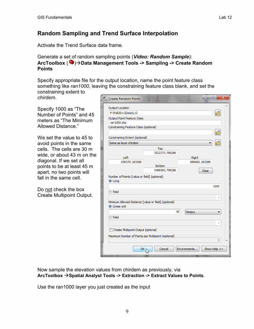
ArcToolbox ( )Data Management Tools -> Sampling -> Create Random Points Specify appropriate file for the output location, name the point feature class something like ran1000, leaving the constraining feature class blank, and set the constraining extent to chirdem. Specify 1000 as “The Number of Points” and 45 meters as “The Minimum Allowed Distance.” We set the value to 45 to avoid points in the same cells. The cells are 30 m wide, or about 43 m on the diagonal. If we set all points to be at least 45 m apart, no two points will fall in the same cell. Do not check the box Create Multipoint Output. Now sample the elevation values from chirdem as previously, via ArcToolbox Spatial Analyst Tools -> Extraction -> Extract Values to Points. Use the ran1000 layer you just created as the input


10

Name the output something like ran1000_with_elevation. Remove the ran1000 data layer. Inspect the table for the ran1000_with_elevation layer table, and note the name of the new column created that contains elevation values. Calculate an interpolation surface, this time using the ArcToolboxSpatial Analyst ToolsInterpolationTrend (Video: Trend Surface) Use the ran1000_with_elevation as your input point data. Save to a permanent output data set named something like trend_p3. Make sure you use the correct column/attribute for the Z value field of the ran1000_with_elevation data set and a cell size of 30. Set the output polynomial order to 3, and the regression type to linear. Run the interpolation, and then load the output interpolated surface into the Trend Surface data view, if it doesn’t load automatically. Create and add contour lines and specify symbology, as you did for the previous interpolation, to yield an output that looks something like that shown at the right.


11

Stratified Random Sampling of a Raster Layer (Video: StratRan1.mov) Sometimes we want to vary the sampling frequency across a map. Here, we’ll place more samples in areas that are steeper. First we’ll create three zones, or strata, and then we’ll assign samples based on these strata. Samples will be assigned proportional to both the area of the strata, and the relative steepness, with more samples in steeper strata. Our strata boundaries will be based on slope, filtered to create larger, more generalized areas. Activate your Spline Stratified Data Frame.

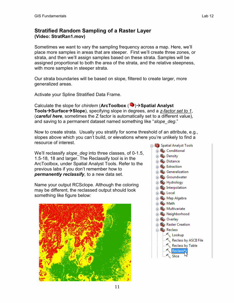
Calculate the slope for chirdem (ArcToolbox ( )Spatial Analyst ToolsSurfaceSlope), specifying slope in degrees, and a z-factor set to 1, (careful here, sometimes the Z factor is automatically set to a different value), and saving to a permanent dataset named something like “slope_deg.” Now to create strata. Usually you stratify for some threshold of an attribute, e.g., slopes above which you can’t build, or elevations where you’re unlikely to find a resource of interest. We’ll reclassify slope_deg into three classes, of 0-1.5, 1.5-18, 18 and larger. The Reclassify tool is in the ArcToolbox, under Spatial Analyst Tools. Refer to the previous labs if you don’t remember how to permanently reclassify, to a new data set. Name your output RCSclope. Although the coloring may be different, the reclassed output should look something like figure below:


12

Now we want to reduce some of the “speckle” in the reclassed slope layer (RCslope). Single pixels or long, thin areas embedded in another strata, and if we place a sample point there, we won’t be stratifying very well. The speckle isn’t bad here, but sometimes it is, and this is a good opportunity to practice smoothing (Video: Prepare Strata Base).

Use ArcToolbox ( ) Spatial Analyst ToolsGeneralizationMajority Filter. Specify a FOUR as the Number of neighbors to use and the HALF replacement threshold.

Your output should look something like the image at the right. Notice how the small speckles are removed in the majority filter output, but the long, thin reaches in valleys remain. Again, this isn’t a great issue here, but in many cases we want very general strata, so we’ll apply another step.


13

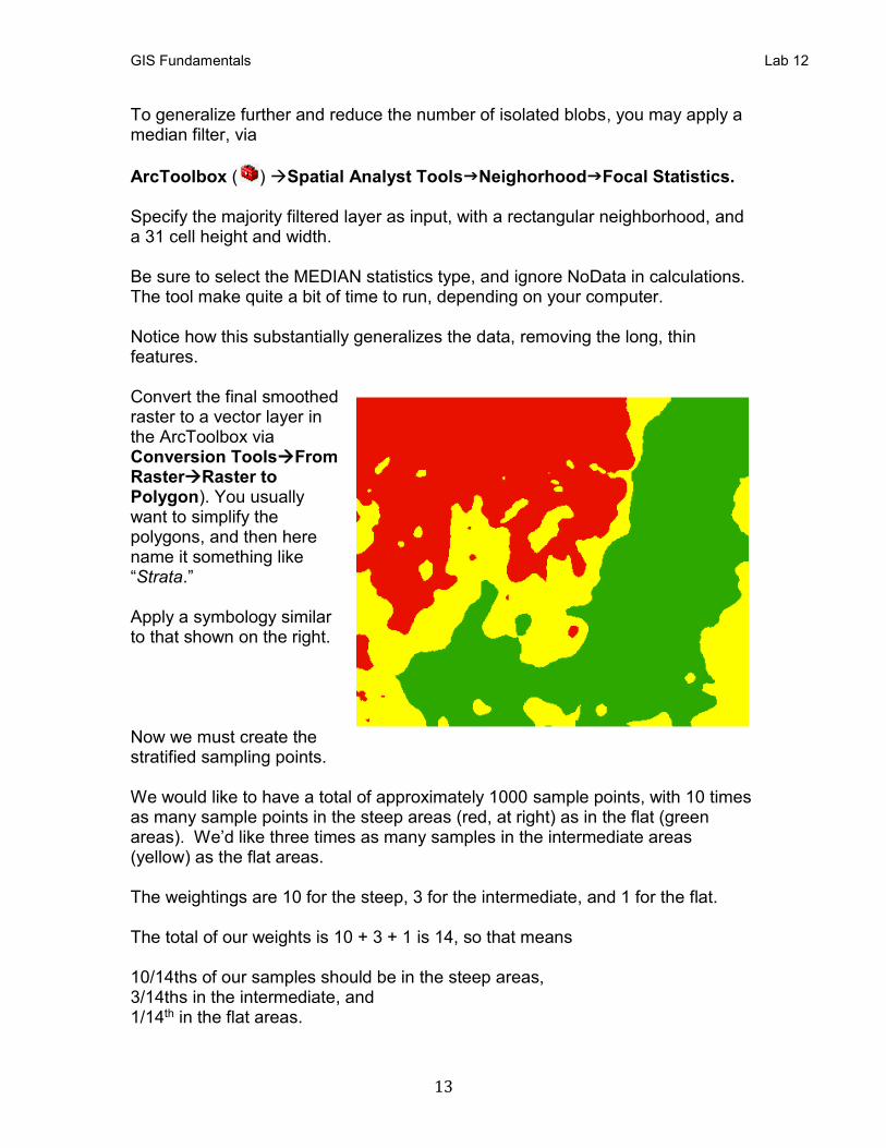
To generalize further and reduce the number of isolated blobs, you may apply a median filter, via

ArcToolbox ( ) Spatial Analyst ToolsNeighorhoodFocal Statistics. Specify the majority filtered layer as input, with a rectangular neighborhood, and a 31 cell height and width. Be sure to select the MEDIAN statistics type, and ignore NoData in calculations. The tool make quite a bit of time to run, depending on your computer. Notice how this substantially generalizes the data, removing the long, thin features. Convert the final smoothed raster to a vector layer in the ArcToolbox via Conversion ToolsFrom RasterRaster to Polygon). You usually want to simplify the polygons, and then here name it something like “Strata.” Apply a symbology similar to that shown on the right. Now we must create the stratified sampling points. We would like to have a total of approximately 1000 sample points, with 10 times as many sample points in the steep areas (red, at right) as in the flat (green areas). We’d like three times as many samples in the intermediate areas (yellow) as the flat areas. The weightings are 10 for the steep, 3 for the intermediate, and 1 for the flat. The total of our weights is 10 + 3 + 1 is 14, so that means 10/14ths of our samples should be in the steep areas, 3/14ths in the intermediate, and 1/14th in the flat areas.


14

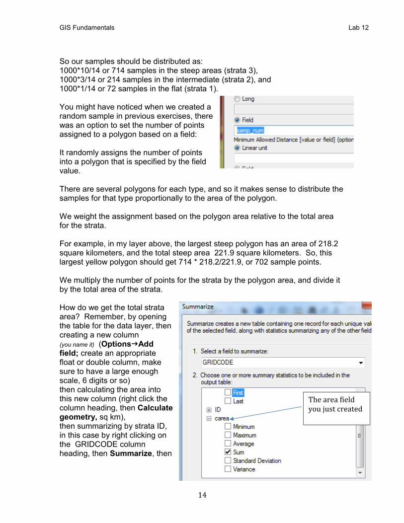
So our samples should be distributed as: 1000*10/14 or 714 samples in the steep areas (strata 3), 1000*3/14 or 214 samples in the intermediate (strata 2), and 1000*1/14 or 72 samples in the flat (strata 1). You might have noticed when we created a random sample in previous exercises, there was an option to set the number of points assigned to a polygon based on a field: It randomly assigns the number of points into a polygon that is specified by the field value. There are several polygons for each type, and so it makes sense to distribute the samples for that type proportionally to the area of the polygon. We weight the assignment based on the polygon area relative to the total area for the strata. For example, in my layer above, the largest steep polygon has an area of 218.2 square kilometers, and the total steep area 221.9 square kilometers. So, this largest yellow polygon should get 714 * 218.2/221.9, or 702 sample points. We multiply the number of points for the strata by the polygon area, and divide it by the total area of the strata. How do we get the total strata area? Remember, by opening the table for the data layer, then creating a new column (you name it) (OptionsAdd field; create an appropriate float or double column, make sure to have a large enough scale, 6 digits or so) then calculating the area into this new column (right click the column heading, then Calculate geometry, sq km), then summarizing by strata ID, in this case by right clicking on the GRIDCODE column heading, then Summarize, then

The area field you just created


15

specifying the sum for carea and an output table. In my case, this results in a calculated area of: -272.6 square kilometers for the flat (gridcode = 1) strata -178.5 square kilometers for the intermediate (gridcode = 2) strata, and -221.9 square kilometers for the steep (gridcode = 3) strata Your numbers may be slightly different, but should be with a few percent of these areas if you used the methods we described above. Write down your summary areas for all three of your classes, you will need them later We now want to calculate the number of samples per polygon. (Video: Stratified Random) Samples per polygon may be computed many ways, but we’ll: 1) Open the strata layer attribute table and add a new long integer field named

samp_num 2) Select all polygons for a given strata (gridcode) 3) Multiply the total number of points for this stratum (e.g., 714 for the steep

strata, gridcode 3) by the area of the polygon, divided by the total area of the strata (in this case 221.9). Repeat this process for strata 2 & 1.

You’ll notice in the calculation shown at right that I’ve added 0.5, and applied the Int () function. We can only assign whole sample points, and add the 0.5 for rounding. Do this for all three strata, substituting the appropriate areas and number of samples for the strata.

The area field you just created


16

Note that your numbers for the strata area and relative number of samples may be different than those shown if you apply a different set of generalization parameters.

Next perform SelectionClear Selected Features. (Video: StratRan4.mov) Now, to create the random points. We use the same tool as before, ArcToolbox -> Data Management Tools -> Sampling -> Create Random Points.

Specify an output location and file name, something like strat_ran, and a Constraining Feature Class as the vector layer called “strata” Make sure to select the Field radio button to specify the number of points, and use the number value column you calculated (samp_num in this example).


17

This should generate a sample set that looks something like that to the right, with a higher sampling density in the steeper areas. Now you should apply this stratified random sample to one last interpolation method. First, use ArcToolbox -> Spatial Analyst Tools -> Extraction -> Extract Values to

Points to assign the chirdem elevation values to each sample point (refer to the previous instructions if need be). Name the output file strat_ran_with_elevation. Next, estimate a surface using a spline interpolation routine, found in the Arc

Tools( ), Spatial Analyst ToolboxInterpolationSpline. Specify the strat_ran_with_elevation as the input for the point features, with the chirdem elevation value field (called rastvalu) as the Z value. Specify an output raster, and set the cell size to equal that of chirdem.

Use a Tension Spline type, with the default weight of 0.1, and use 20 points for the spline. After running the tool, add this output to your data frame. Calculate contours, and display these and the sample points on your layout. Arrange the layout so it looks approximately like that in the figure below, with an appropriate title, labels, scalebar, name, uniform elevation legend across all three interpolation layers, and north arrow, and turn this in.


18


19

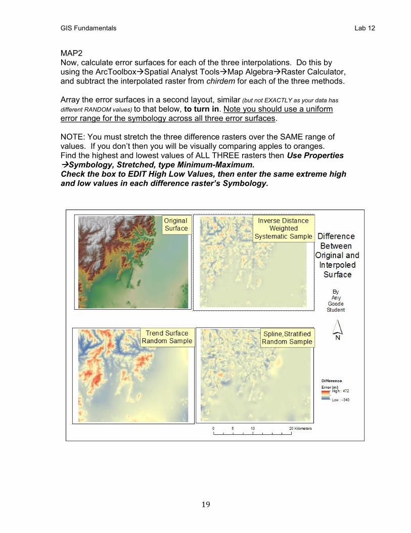
MAP2 Now, calculate error surfaces for each of the three interpolations. Do this by using the ArcToolboxSpatial Analyst ToolsMap AlgebraRaster Calculator, and subtract the interpolated raster from chirdem for each of the three methods. Array the error surfaces in a second layout, similar (but not EXACTLY as your data has

different RANDOM values) to that below, to turn in. Note you should use a uniform error range for the symbology across all three error surfaces. NOTE: You must stretch the three difference rasters over the SAME range of values. If you don’t then you will be visually comparing apples to oranges. Find the highest and lowest values of ALL THREE rasters then Use Properties Symbology, Stretched, type Minimum-Maximum. Check the box to EDIT High Low Values, then enter the same extreme high and low values in each difference raster’s Symbology.

lab 12: sampling and interpolation - gis courses 12: sampling and interpolation what you ......

Documents