l5: digital filters - texas a&m...

Introduction to Speech Processing | Ricardo Gutierrez-Osuna | CSE@TAMU 1

L5: Digital filters

• Linear time invariant systems

• Impulse response

• Transfer function

• Digital filter analysis

• Example: speech synthesis

This lecture is based on chapter 10 of [Taylor, TTS synthesis, 2009]


Filters

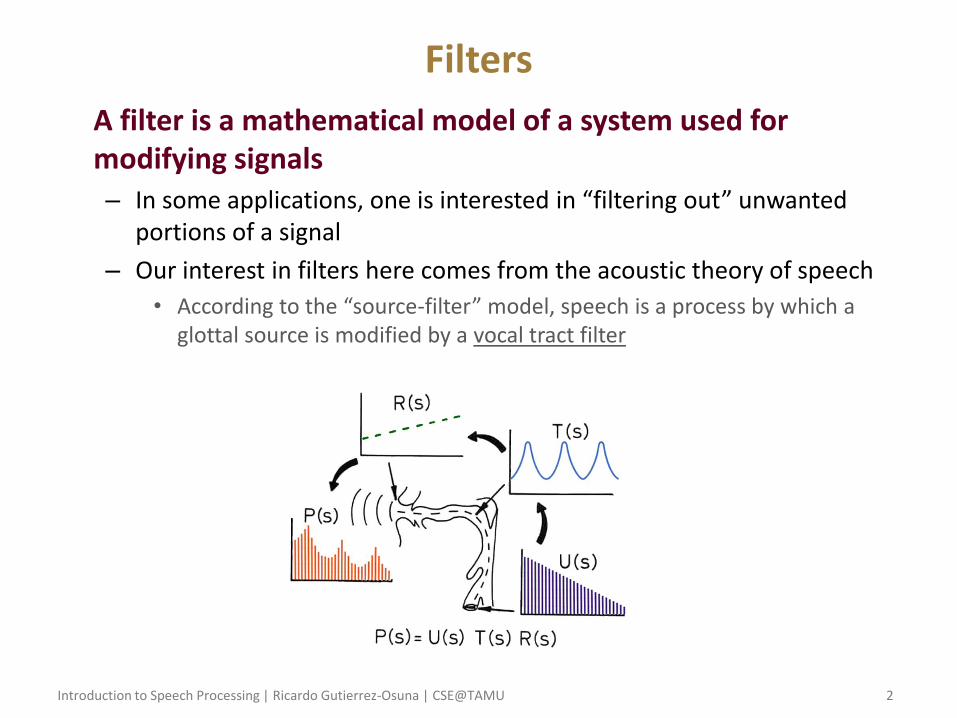
• A filter is a mathematical model of a system used for modifying signals – In some applications, one is interested in “filtering out” unwanted

portions of a signal

– Our interest in filters here comes from the acoustic theory of speech

• According to the “source-filter” model, speech is a process by which a glottal source is modified by a vocal tract filter


• Linear time invariant (LTI) filters – A class of linear filters whose behavior does not change over time

• Linearity implies that the filter meets the scaling and superposition properties

𝑥 𝑛 ↦ 𝑦 𝑛 ⟹ 𝛼𝑥1 𝑛 + 𝛽𝑥2 𝑛 ↦ 𝛼𝑦1 𝑛 + 𝛽𝑦2 𝑛

– LTI filters are generally described in terms of difference equations

• Types of LTI filters – Finite impulse response (FIR)

• Operate only on previous values of the input

𝑦 𝑛 = 𝑏𝑘𝑥 𝑛 − 𝑘𝑀

𝑘=0

– Infinite impulse response (IIR)

• Operate as well on previous values of the output

𝑦 𝑛 = 𝑏𝑘𝑥 𝑛 − 𝑘𝑀

𝑘=0+ 𝑎𝑙𝑦 𝑛 − 𝑙

𝑁

𝑙=0


http://www.mikroe.com/eng/chapters/view/73/chapter-3-iir-filters/


• The impulse response – The properties of a filter in the time domain can be described by its

response when the input is an impulse

𝛿 𝑛 = 0 𝑛 = 01 𝑛 ≠ 0

– Consider the IIR filter defined by 𝑦 𝑛 = 𝑥 𝑛 − 0.8𝑦 𝑛 − 1

• Impulse response has no fixed duration (it is infinite, hence the name)

• The response is an exponential decay controlled by 𝑎1 = −0.8

– For 𝑎1 > 1, output grows exponentially, and the filter is said to be unstable

– Now consider the IIR filter 𝑦 𝑛 = −1.8𝑦 𝑛 − 1 + 𝑦 𝑛 − 2

• In this case, the response has the shape of a sine wave

– Finally, consider the IIR filter 𝑦 𝑛 = −1.78𝑦 𝑛 − 1 + 0.9𝑦 𝑛 − 2

• In this case, the response has the shape of a decaying sine wave, a mix of the previous two signals

– Thus, the response characteristics are entirely defined by the parameters of the filter


• Example

ex5p1.m Generate example of IIR and FIR filters Show how the impulse response is

infinite for IIR but finite for FIR (examples from Taylor §10.4.1-2)


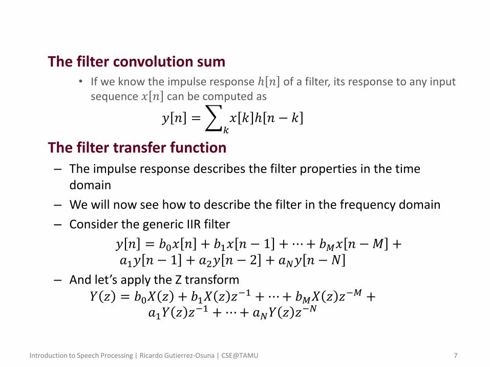
• The filter convolution sum • If we know the impulse response ℎ 𝑛 of a filter, its response to any input

sequence 𝑥 𝑛 can be computed as

𝑦 𝑛 = 𝑥 𝑘 ℎ 𝑛 − 𝑘𝑘

• The filter transfer function – The impulse response describes the filter properties in the time

domain

– We will now see how to describe the filter in the frequency domain

– Consider the generic IIR filter

𝑦 𝑛 = 𝑏0𝑥 𝑛 + 𝑏1𝑥 𝑛 − 1 + ⋯+ 𝑏𝑀𝑥 𝑛 − 𝑀 + 𝑎1𝑦 𝑛 − 1 + 𝑎2𝑦 𝑛 − 2 + 𝑎𝑁𝑦 𝑛 − 𝑁

– And let’s apply the Z transform 𝑌 𝑧 = 𝑏0𝑋 𝑧 + 𝑏1𝑋 𝑧 𝑧−1 + ⋯+ 𝑏𝑀𝑋 𝑧 𝑧−𝑀 +

𝑎1𝑌 𝑧 𝑧−1 + ⋯+ 𝑎𝑁𝑌 𝑧 𝑧−𝑁


– which, grouping terms, can be expressed as

𝑌 𝑧 =𝑏0 + 𝑏1𝑧

−1 + ⋯+ 𝑏𝑀𝑧𝑀−1

1 − 𝑎1𝑧−1 − ⋯− 𝑎𝑁𝑧𝑁−1

𝑋 𝑧

– from which the transfer function of the filter can be defined as:

𝐻 𝑧 =𝑌 𝑧

𝑋 𝑧=

𝑏𝑘𝑧−𝑘𝑀

𝑘=0

𝑎𝑙𝑧−𝑙𝑁

𝑙=0

• NOTES – As we will see in the next few slides, the transfer function 𝐻 𝑧 fully

defines the filter’s characteristics in the frequency domain

– It can be shown that the transfer function is the Z-transform of the impulse response 𝐻 𝑧 = ℎ 𝑘 𝑧−𝑘

– The transfer function is a ratio of two polynomials whose coefficients are those of the difference equation


Filter analysis and design

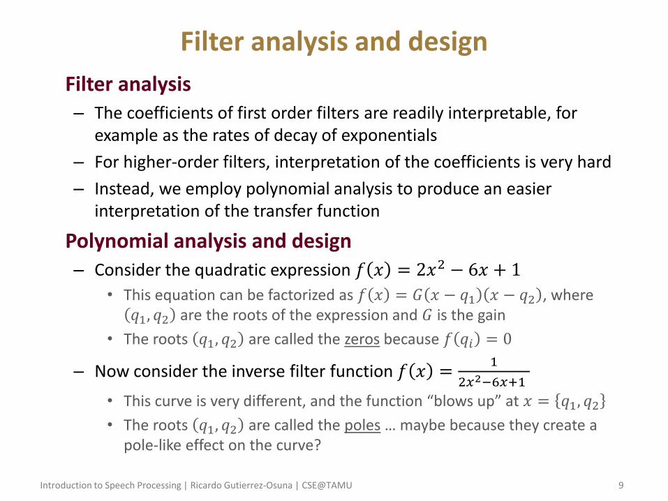
• Filter analysis – The coefficients of first order filters are readily interpretable, for

example as the rates of decay of exponentials

– For higher-order filters, interpretation of the coefficients is very hard

– Instead, we employ polynomial analysis to produce an easier interpretation of the transfer function

• Polynomial analysis and design – Consider the quadratic expression 𝑓 𝑥 = 2𝑥2 − 6𝑥 + 1

• This equation can be factorized as 𝑓 𝑥 = 𝐺 𝑥 − 𝑞1 𝑥 − 𝑞2 , where 𝑞1, 𝑞2 are the roots of the expression and 𝐺 is the gain

• The roots 𝑞1, 𝑞2 are called the zeros because 𝑓 𝑞𝑖 = 0

– Now consider the inverse filter function 𝑓 𝑥 =1

2𝑥2−6𝑥+1

• This curve is very different, and the function “blows up” at 𝑥 = 𝑞1, 𝑞2

• The roots 𝑞1, 𝑞2 are called the poles … maybe because they create a pole-like effect on the curve?


[Taylor, 2009]


– We can now use polynomials to analyze our filter’s transfer function

– Consider the transfer function

𝐻 𝑧 =1

𝑧2 − 𝑎1𝑧 −𝑎2

– Since transfer functions are generally expressed in terms of 𝑧−1, we multiply numerator and denominator by 𝑧−2 to obtain

𝐻 𝑧 =𝑧−2

1 − 𝑎1𝑧−1 − 𝑎2𝑧

−2= 𝐺

𝑧−2

1 − 𝑝1𝑧−1 1 − 𝑝2𝑧

−2

– The figures in the next slide show the shape of the transfer function for 𝑎1 = 1, 𝑎2 = −0.5

• In this case the roots of the denominator are complex 0.5 ± 𝑗0.5

• Note how the shape of the filter can be described by the position of the poles in the Z plane; we do not need to plot 𝐻(𝑧)


[Taylor, 2009]


– The same analysis can be extended to any LTI filter

𝐻 𝑧 =𝑏0 + 𝑏1𝑧

−1 + ⋯+ 𝑏𝑀𝑧𝑀

1 − 𝑎1𝑧−1 − ⋯− 𝑎𝑁𝑧𝑁

– By expressing it in terms of its factors

𝐻 𝑧 =1 − 𝑞1𝑧

−1 1 − 𝑞2𝑧−1 … 1 − 𝑞𝑀𝑧−1

1 − 𝑝1𝑧−1 1 − 𝑝2𝑧

−1 … 1 − 𝑝𝑁𝑧−1

– And then analyzing the position of its poles and zeros in the Z plane


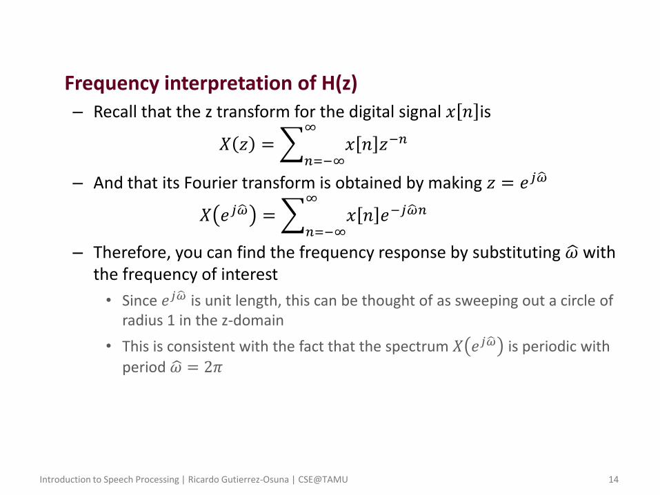
• Frequency interpretation of H(z) – Recall that the z transform for the digital signal 𝑥 𝑛 is

𝑋 𝑧 = 𝑥 𝑛 𝑧−𝑛∞

𝑛=−∞

– And that its Fourier transform is obtained by making 𝑧 = 𝑒𝑗𝜔

𝑋 𝑒𝑗𝜔 = 𝑥 𝑛 𝑒−𝑗𝜔 𝑛∞

𝑛=−∞

– Therefore, you can find the frequency response by substituting 𝜔 with the frequency of interest

• Since 𝑒𝑗𝜔 is unit length, this can be thought of as sweeping out a circle of radius 1 in the z-domain

• This is consistent with the fact that the spectrum 𝑋 𝑒𝑗𝜔 is periodic with

period 𝜔 = 2𝜋


[Taylor, 2009]


• Filter characteristics – Consider the following first-order IIR filter

ℎ 𝑛 = 𝑏0𝑥 𝑛 − 𝑎1𝑦 𝑛 − 1

𝐻 𝑧 =𝑏0

1 − 𝑎1𝑧−1

=𝑏0

1 − 𝑎1𝑒−𝑗𝜔

– The figures in the next page show the time- and frequency domain response, pole locations and pole locations in the z-domain for 𝑏1 = 1 and 𝑎1 = 0.8,0.7,0.6,0.4

• This type of filter is known as a resonator, and the peak is known as a resonance because frequencies near that peak are amplified by the filter

– Analysis

• As the length of the decay increases, the peak becomes sharper

• Large 𝑎1 corresponds to slow decays and narrow bandwidths

• Small 𝑎1 corresponds to fast decays and broad bandwidths


[Taylor, 2009]


– Resonances are generally described by three properties: amplitude, frequency, and bandwidth

• The radius of the pole controls the amplitude and bandwidth

• The angle of the pole controls the frequency; in this case 𝜔 = 0 since the pole lies on the real line

– In order to model speech resonances at non-zero frequencies, we then move the pole away from the real axis

• This will result in a complex pole 𝑝1 = 𝑟𝑒𝑗𝜃 = 𝛼 + 𝑗𝛽, which leads to a complex filter coefficient 𝑎1; see next slide

• For this reason, we introduce complex-conjugate pairs of poles 𝑟𝑒±𝑗𝜃

𝐻 𝑧 =1

1 − 𝑟𝑒𝑗𝜃𝑧−1 1 − 𝑟𝑒−𝑗𝜃𝑧−1=

1

1 − 2𝑟𝑐𝑜𝑠 𝜃 𝑧−1 + 𝑟2𝑧−1

– Examples for various pole positions are shown in the next slide

• For constant 𝜃, the filter becomes sharper as 𝑟 → 1

– For small 𝑟, the skirts of the two poles overlap and shift the resonance

• For constant 𝑟, resonances move away from 𝜔 = 0 as 𝜃 → 1


[Taylor, 2009]


– Effect of zeros

• Adding a term 𝑏1 = 1 places a zero at the origin

• Adding a term 𝑏1 = −1 places a zero at the ends of the spectrum

– Thus, zeros add anti-resonances to the spectrum

𝑏1 = 1 𝑏1 = −1


– Thus, we can build any transfer function by placing poles and zeros at the appropriate locations and then multiplying their transfer functions

– Note, though, that poles that are close together will interact, so the final resonances of a system cannot always be predicted from their poles


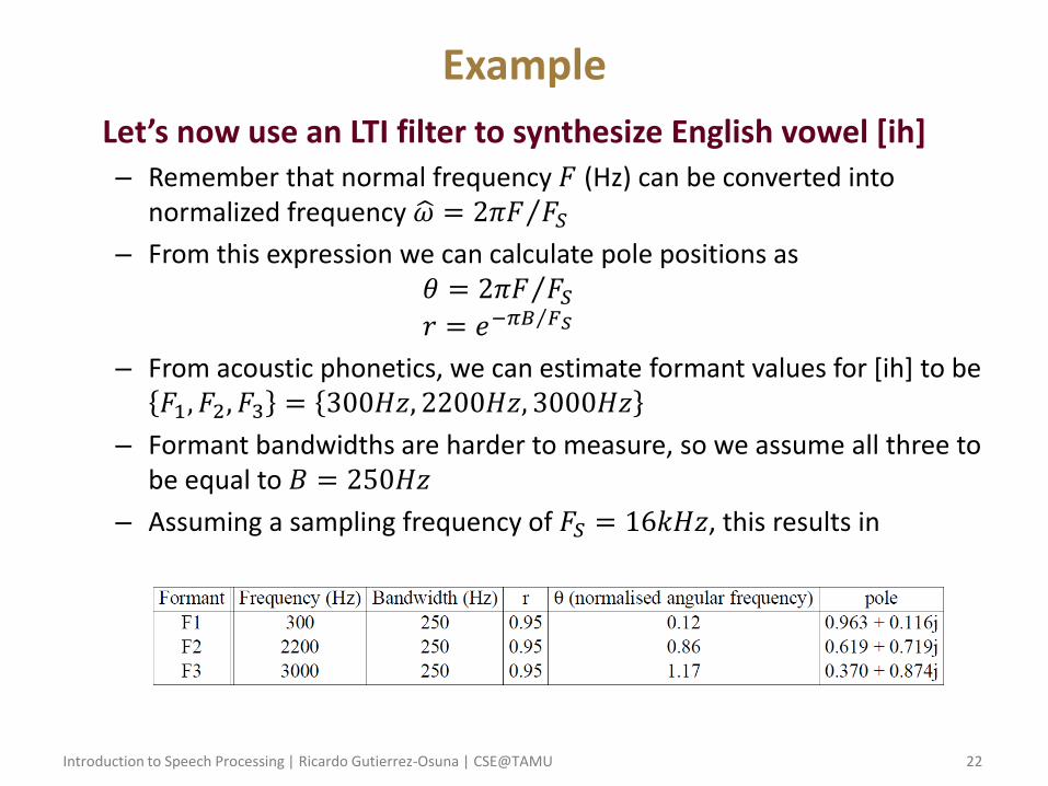
Example

• Let’s now use an LTI filter to synthesize English vowel [ih] – Remember that normal frequency 𝐹 (Hz) can be converted into

normalized frequency 𝜔 = 2𝜋𝐹 𝐹𝑆

– From this expression we can calculate pole positions as 𝜃 = 2𝜋𝐹 𝐹𝑆

𝑟 = 𝑒−𝜋𝐵 𝐹𝑆

– From acoustic phonetics, we can estimate formant values for [ih] to be 𝐹1, 𝐹2, 𝐹3 = 300𝐻𝑧, 2200𝐻𝑧, 3000𝐻𝑧

– Formant bandwidths are harder to measure, so we assume all three to be equal to 𝐵 = 250𝐻𝑧

– Assuming a sampling frequency of 𝐹𝑆 = 16𝑘𝐻𝑧, this results in


– The transfer function for each formant can be estimated as

𝐻𝑛 𝑧 =1

1 − 𝑝𝑛𝑧−1 1 − 𝑝𝑛

∗𝑧−1

– And the complete vocal tract TF can be estimated by multiplication 𝐻 𝑧 = 𝐻1 𝑧 𝐻2 𝑧 𝐻3 𝑧


• Example

ex5p2.m Synthesize speech sample using the previous vocal tract filter and a pulse train as glottal excitation

l5: digital filters - texas a&m...

Documents