l1regularizaon&introtolearningtheory lecture8ent:# eligibilityrecord: cmember&id& ......
TRANSCRIPT

L1 regulariza,on & Intro to learning theory Lecture 8
David Sontag New York University

Feature Selec9on Se7ng: Lots of possible features, many of which are irrelevant
Example:
When studying depression in teens, a researcher distributes a ques9onnaire of 250 different ques9ons, many of them related or irrelevant.
Goal: Find a small set of ques9ons that can be used to quickly determine whether or not a teen is depressed.
Mathema9cally:
min
w`(w · x, y) + �(non-zero elements in w)

L1 regulariza9on
• Penalizing the L1 norm of the weight vector leads to sparse (read: many 0’s) solu9ons for w.
• Why?
minw
`(w · x, y) + �|w|

L1 regulariza9on
• Penalizing the L1 norm of the weight vector leads to sparse (read: many 0’s) solu9ons for w.
• Why?
minw
`(w · x, y) + �|w|Minimize this:
Subject to Constant L1 norm
Subject to Constant L2 norm

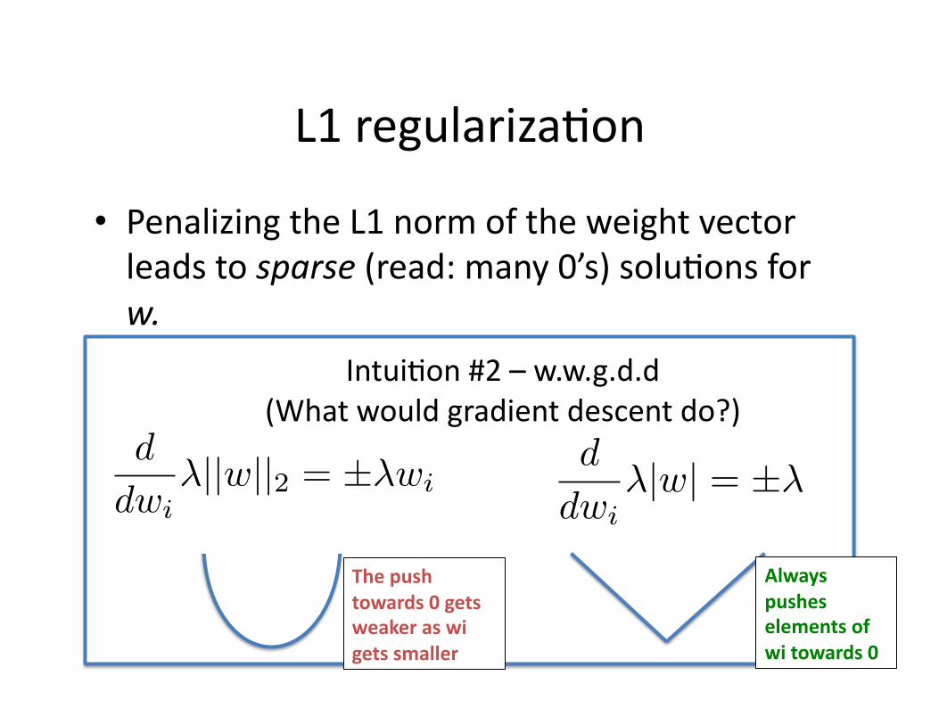
• Penalizing the L1 norm of the weight vector leads to sparse (read: many 0’s) solu9ons for w.
• Why?
minw
`(w · x, y) + �|w|Intui9on #2 – w.w.g.d.d (What would gradient descent do?)
d
dwi�|w| = ±�
L1 regulariza9on
d
dwi�||w||2 = ±�wi
• Penalizing the L1 norm of the weight vector leads to sparse (read: many 0’s) solu9ons for w.
• Why?
minw
`(w · x, y) + �|w|Intui9on #2 – w.w.g.d.d (What would gradient descent do?)
d
dwi�|w| = ±�
L1 regulariza9on
d
dwi�||w||2 = ±�wi
The push towards 0 gets weaker as wi gets smaller
Always pushes elements of wi towards 0

Example: Early Detec,on of Type 2 Diabetes
• Global prevalence will go from 171 million in 2000 to 366 million in 2030
• 25% of people in the US with diabetes are undiagnosed
• Leads to complica9ons of cardiovascular, cerebrovascular, renal, and vision systems
• Early lifestyle changes shown to prevent or delay the onset of the disease be]er than Me^ormin

Tradi9onal risk
assessment
• Use small number of risk factors (e.g. ~20)
• Easy to ask/measure in the office
• Simple model: can calculate scores by hand

Popula9on-‐Level Risk Stra9fica9on
• Key idea: Use automa9cally collected administra9ve, u9liza9on, and clinical data
• Machine learning will find surrogates for risk factors that would otherwise be missing
• Enables risk stra9fica9on at the popula9on level – millions of pa9ents
[N. Razavian, S. Blecker, A.M. Schmidt, A. Smith-‐McLallen, S. Nigam, D. Sontag. Popula9on-‐Level Predic9on of Type 2 Diabetes using Claims Data and Analysis of Risk Factors. Big Data, Jan. 2016.]

Administra9ve & Clinical Data
Pa,ent:
Eligibility Record: -‐Member ID -‐Age/gender -‐ID of subscriber -‐Company code
Medical Claims: -‐ICD9 diagnosis code -‐CPT code (procedure) -‐Specialty -‐Loca9on of service -‐Date of Service
Lab Tests: -‐LOINC code (urine or blood test name) -‐Results (actual values) -‐Lab ID -‐Range high/low-‐Date
Medica,ons: -‐NDC code (drug name) -‐Days of supply -‐Quan9ty -‐Service Provider ID -‐Date of fill
,me

1) Training Step (model fi7ng)
Machine Learning Task: predict the probability of a member developing diabetes
Training Data: Member Informa,on
Training Labels: Has the member developed Type 2 diabetes within the predic,on window?
Op,mize Model Parameters Model: L1 Regularized Logis5c Regression
Representa,on as a set of feature vectors
2) Predic,on Step
New member’s data Representa,on as a feature vector
Predict the label for the New Pa5ent
Model Parameters
650,000 members’ data

22 risk factors derived from literature (age, sex, obesity, fas9ng glucose level, cardiovascular disease, hypertension, …)
39 coverage features
457 procedure groups
228 special,es (cardiology, rheumatology, …)
Features 32 service places (urgent care, inpa9ent, outpa9ent, …)
7000 laboratory indicators
For the 1000 most frequent lab tests: • Was the test ever administered? • Was the result ever low? • Was the result ever high? • Was the result ever normal? • Is the value increasing? • Is the value decreasing? • Is the value fluctua9ng?
999 medica,on groups (laxa9ves, me^ormin, an9-‐arthri9cs, …)

22 risk factors derived from literature (age, sex, obesity, fas9ng glucose level, cardiovascular disease, hypertension, …)
39 coverage features
457 procedure groups
228 special,es (cardiology, rheumatology, …)
Features 32 service places (urgent care, inpa9ent, outpa9ent, …)
7000 laboratory indicators
999 medica,on groups (laxa9ves, me^ormin, an9-‐arthri9cs, …)
16,000 ICD-‐9 diagnosis codes (all history)
All history 24 month history
6 month history
Total features per pa,ent: 42,000

What are the discovered risk factors?
Feature Name Impaired Fasting Glucose (790.21) Abnormal Glucose NEC (790.29) Hypertension (401) Obstructive Sleep Apnea (327.23) Obesity (278) Abnormal Blood Chemistry (790.6) Hyperlipidemia (272.4) Shortness Of Breath (786.05) Esophageal Reflux (530.81) Acute Bronchitis (466.0) Actinic Keratosis (702.0)
Diagnos9c groups Procedure Group Lab Test Medica9on Group Service Place
Addi,onal risk factors iden_ied: Impaired oral glucose tolerance, Chronic liver disease, Pituitary dwarfism, Hypersomnia with sleep apnea, Joint replaced knee, Liver disorder, Iron deficiency anemia, Mitral valve disorder…
Posi,ve weights

What are the discovered risk factors?
Feature Name Hemoglobin A1c / Hemoglobin.Total - High Glucose - High Hemoglobin A1c / Hemoglobin.Total - Request For Test Cholesterol.In HDL - Low Cholesterol.Total / Cholesterol.In HDL - High Cholesterol.In VLDL - Request For Test Carbon Dioxide - Request For Test Glomerular Filtration Rate/1.73 Sq. M. Predicted Black - Request For Test
Diagnos9c groups Procedure Group Lab Test Medica9on Group Service Place
Addi,onal risk factors iden_ied: Potassium (low), Erythrocyte mean corpuscular hemoglobin concentra9on (fluctua9ng), Erythrocyte distribu9on width (high), Alanine aminotransferase (high), Cholesterol.in LDL (increasing), Crea9nine (decreasing), Albumin/Globulin (increasing)…
Posi,ve weights

What are the discovered risk factors?
Feature Name Routine Chest Xray Medication Group: Anti-arthritics Service Place: Emergency Room - Hospital Routine Medical Exam (V700) Routine Gynecological Examination (V7231) Routine Child Health Exam (V202 )
Diagnos9c groups Procedure Group Lab Test Medica9on Group Service Place
~700 risk factors selected for model
Very nega,ve
Very posi,ve

Type 2 Diabetes Predic9on Accuracy Using pa9ent data through Dec. 31, 2008, who will be newly diagnosed with Type 2 diabetes in the following years?
Model AUC Top 1000 predictions
Top 10000 predictions
Sensitivity Specificity PPV Sensitivity Specificity PPV
Literature features only 0.75 0.014 0.996 0.1 0.114 0.967 0.08
Overall Model 0.8 0.033 0.997 0.24 0.212 0.969 0.14
Literature features only 0.72 0.013 0.995 0.04 0.116 0.957 0.03
Overall Model 0.76 0.023 0.995 0.07 0.179 0.958 0.05
Area under the ROC curve (AUC) = Randomly choosing two members, one who did get diabetes and one who did not, can we predict which is which?
Highest risk popula9on
2 years lead 9me for this popula9on
2009-‐2011 (incident diabetes)
2011-‐2013 (future diabe9cs)

Type 2 Diabetes Predic9on Accuracy

Type 2 Diabetes Predic9on Accuracy Using pa9ent data through Dec. 31, 2008, who will be newly diagnosed with Type 2 diabetes in the following years?
Model AUC Top 1000 predictions
Top 10000 predictions
Sensitivity Specificity PPV Sensitivity Specificity PPV
Literature features only 0.75 0.014 0.996 0.1 0.114 0.967 0.08
Overall Model 0.8 0.033 0.997 0.24 0.212 0.969 0.14
Literature features only 0.72 0.013 0.995 0.04 0.116 0.957 0.03
Overall Model 0.76 0.023 0.995 0.07 0.179 0.958 0.05
2009-‐2011 (incident diabetes)
2011-‐2013 (future diabe9cs)
Sensitivity = TP/P “true positive rate” or “recall”
Specificity = TN/N “true negative rate”
PPV = TP/(TP+FP) “positive predictive value”

Type 2 Diabetes Predic9on Accuracy
2009-‐2011 (incident diabetes)
2011-‐2013 (future diabe9cs)
Using pa9ent data through Dec. 31, 2008, who will be newly diagnosed with Type 2 diabetes in the following years?
Model AUC Top 1000 predictions
Top 10000 predictions
Sensitivity Specificity PPV Sensitivity Specificity PPV
Literature features only 0.75 0.014 0.996 0.1 0.114 0.967 0.08
Overall Model 0.8 0.033 0.997 0.24 0.212 0.969 0.14
Literature features only 0.72 0.013 0.995 0.04 0.116 0.957 0.03
Overall Model 0.76 0.023 0.995 0.07 0.179 0.958 0.05

What’s next… • We gave several machine learning algorithms:
– Perceptron
– Linear support vector machine (SVM)
– SVM with kernels, e.g. polynomial or Gaussian
• How do we guarantee that the learned classifier will perform well on test data?
• How much training data do we need?

Example: Perceptron applied to spam classifica9on
• In your homework 1, you trained a spam classifier using perceptron – The training error was always zero – With few data points, there is a big gap between training error and
test error!
Number of training examples
Test error (percentage misclassified)
Test error -‐ training error > 0.065
Test error -‐ training error < 0.02

How much training data do you need?
• Depends on what hypothesis class the learning algorithm considers
• For example, consider a memoriza9on-‐based learning algorithm – Input: training data S = { (xi, yi) } – Output: func9on f(x) which, if there exists (xi, yi) in S such that x=xi, predicts yi,
and otherwise predicts the majority label – This learning algorithm will always obtain zero training error
– But, it will take a huge amount of training data to obtain small test error (i.e., its generaliza9on performance is horrible)
• Linear classifiers are powerful precisely because of their simplicity – Generaliza9on is easy to guarantee

1. Generaliza9on of finite hypothesis spaces
2. VC-‐dimension
• Will show that linear classifiers need to see approximately d training points, where d is the dimension of the feature vectors
• Explains the good performance we obtained using perceptron!!!! (we had a few thousand features)
3. Margin based generaliza9on
• Applies to infinite dimensional feature vectors (e.g., Gaussian kernel)
Number of training examples
Test error (percentage misclassified)
Perceptron algorithm on spam classifica9on
Roadmap of next lectures
[Figure from Cynthia Rudin]