l1 adaptive controller for a missile longitudinal ...ccao/caopaper/wangaiaa08l1.pdf · this paper...

L1 Adaptive Controller for a Missile Longitudinal Autopilot

Design

Jiang Wang∗

Virginia Tech, Blacksburg, VA 24061, USA

Chengyu Cao†

University of Connecticut, Storrs, CT, 06269, USA

Naira Hovakimyan‡

University of Illinois at Urbana-Champaign, Urbana, IL 61801, USA

Richard E. Hindman§ and D. Brett Ridgely¶

Raytheon Missile Systems, Tucson, AZ 85734, USA

This paper considers application ofL1 adaptive output feedback controller to a missile longitudinal au-

topilot design. The proposed adaptive controller has satisfactory performance in the presence of parametric

uncertainties and time-varying disturbances. Simulations demonstrate the benefits of the control method and

compare the results to Linear Quadratic Regulator (LQR) and Linear Quadratic Gaussian (LQG) with Loop

Transfer Recovery (LTR) design.

I. Introduction

This paper presents the application of anL1 adaptive output feedback controller to longitudinal autopilot design

for a missile in the presence of uncertainties in system dynamics. The uncertainties include parametric variations in

the transfer function and time-varying disturbances. The parametric variations of the system’s transfer function are

caused by changes in aerodynamic coefficients. The missile model, taken from Mracek and Ridgely [1], is an unstable

non-minimum phase system. The nominal optimal controller in Mracek and Ridgely [1] uses both system outputs

(pitch rate and normal acceleration) to compute the feedback control signal. In this paper we only use the acceleration.

The proposed adaptive output feedback controller, taken from Cao and Hovakimyan [2, 3], allows tracking of

reference systems that do not verify the SPR condition for their input-output transfer functions. Similar to the earlier∗Graduate Research Assistant, Student Member AIAA, Department of Aerospace and Ocean Engineering, 215 Randolph

Hall; [email protected] (Corresponding Author).†Research Assistant Professor, Member AIAA,Department of Mechanical Engineering; [email protected]‡Professor, Associate Fellow AIAA, Department of Mechanical Science and Engineering; [email protected]§Principal Systems Engineer, Member AIAA, [email protected]¶Senior Department Manager, Senior Member AIAA, [email protected]

1 of 21

American Institute of Aeronautics and Astronautics

AIAA Guidance, Navigation and Control Conference and Exhibit18 - 21 August 2008, Honolulu, Hawaii

AIAA 2008-6282

Copyright © 2008 by Jiang Wang. Published by the American Institute of Aeronautics and Astronautics, Inc., with permission.

results of Cao and Hovakimyan [4], theL∞-norms of both input/output error signals between the closed-loop adaptive

system and the reference system can be rendered arbitrarily small by reducing the step-size of integration. The key

difference between [2,3] and [4] is the new piece-wise continuous adaptive law which enables tracking of the reference

systems without imposing the SPR requirement on their input-output transfer function. The adaptive control is defined

as the output of a low-pass filter, resulting in a continuous signal despite the discontinuity of the adaptive law. TheL1

adaptive output feedback controller aims at achieving a guaranteed transient performance for the system’s output, and

regulating the frequency spectrum and the performance bound for the system’s input signal as well, by rendering them

arbitrarily close to the corresponding output/input signals of a bounded reference system.

We consider the longitudinal dynamics of a missile in the presence of uncertainties in aerodynamics and time-

varying disturbances. For comparison purposes, we first consider the nominal optimal controller from Mracek and

Ridgely [1], which is a “classic” three-loop topology autopilot designed by LQR methods. Then assuming only

measured acceleration is available, we design a LQG controller with Loop Transfer Recovery (LTR) to recover the

robustness of the LQR controller. This serves as the nominal output feedback controller in the absence of uncertain-

ties. We augment the baseline LQG controller byL1 adaptive output feedback loop to compensate for the modeling

uncertainties.

The paper is organized as follows. Section II presents the problem formulation. Section III shows the nominal

controller design. Section IV gives an overview of the key results from Cao and Hovakimyan [2, 3], and Section V

discusses some design solutions to achieve the desired performance specifications. Section VI presents the simulations,

while Section VII concludes the paper.

II. Problem Formulation

The missile’s longitudinal dynamics can be described using the short period approximation of the longitudinal

equations of motion [1]:

xp(t) = Apxp(t) + Bp [δp(t) + v(t, y(t))] (1)

yp(t) = Cpxp(t) + Dp [δp(t) + v(t, y(t))] (2)

y(t) = Azm(t) , (3)

whereδp(t) is the elevator input,v(t, y(t)) is time-varying disturbance and depends ony(t), xp(t) andyp(t) are the

state and the output vectors respectively, given by

xp(t) =

α(t)

q(t)

, yp(t) =

Azm(t)

qm(t)

, (4)

2 of 21


while α(t) is angle of attack,q(t) is pitch rate,Azm(t) is normal acceleration andqm(t) is measured pitch rate. In (1)

and (2) the system matrices are

Ap =

1Vm0

[QSCzα0

m −AX0

]1

QSdCmα0IY Y

0

, Bp =

QSCzδp0mVm0

QSdCmδp0IY Y

,

Cp =

QSCzα0mg − QSdCmα0 x

gIY Y0

0 1

, Dp =

QSCzδp0mg − QSdCmδp0

x

gIY Y

0

.

The numerical values of the simulation example in this paper are listed in Table 1, and are taken from Mracek and

Ridgely [1]. In this paper we consider uncertainties in the aerodynamic coefficientsCzα0 , Cmα0 , Czδp0andCmδp0

.

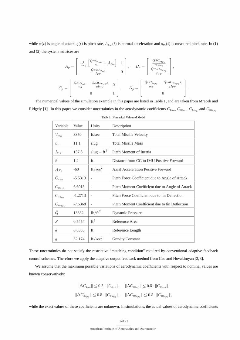
Table 1. Numerical Values of Model

Variable Value Units Description

Vm0 3350 ft/sec Total Missile Velocity

m 11.1 slug Total Missile Mass

IY Y 137.8 slug − ft2 Pitch Moment of Inertia

x 1.2 ft Distance from CG to IMU Positive Forward

AX0 -60 ft/sec2 Axial Acceleration Positive Forward

Czα0 -5.5313 - Pitch Force Coefficient due to Angle of Attack

Cmα0 6.6013 - Pitch Moment Coefficient due to Angle of Attack

Czδp0-1.2713 - Pitch Force Coefficient due to fin Deflection

Cmδp0-7.5368 - Pitch Moment Coefficient due to fin Deflection

Q 13332 lb/ft2 Dynamic Pressure

S 0.5454 ft2 Reference Area

d 0.8333 ft Reference Length

g 32.174 ft/sec2 Gravity Constant

These uncertainties do not satisfy the restrictive “matching condition” required by conventional adaptive feedback

control schemes. Therefore we apply the adaptive output feedback method from Cao and Hovakimyan [2,3].

We assume that the maximum possible variations of aerodynamic coefficients with respect to nominal values are

known conservatively:

‖∆Czα0‖ ≤ 0.5 · ‖Czα0‖, ‖∆Cmα0‖ ≤ 0.5 · ‖Cmα0‖,

‖∆Czδp0‖ ≤ 0.5 · ‖Czδp0

‖, ‖∆Cmδp0‖ ≤ 0.5 · ‖Cmδp0

‖,

while the exact values of these coefficients are unknown. In simulations, the actual values of aerodynamic coefficients

3 of 21


are selected to be

C ′zα0= 1.4 · Czα0

, C ′mα0= 1.4 · Cmα0

, C ′zδp0= 0.7 · Czδp0

, C ′mδp0= 0.7 · Cmδp0

. (5)

The control objective is to design adaptive output feedback controller to achieve satisfactory tracking performance

for the outputAzm(t), in the presence of parametric uncertainties and time-varying disturbances, using onlyAzm(t).

III. Nominal Controller Design

III.A. LQR solution

We first develop the “classical” three-loop topology for the nominal controller design [1], assuming that the required

output signals in the three-loop topology are available. The system is augmented by consideringz(t) = δp(t) +

v(t, y(t)) as an additional state:

x1(t) = A1x1(t) + B1 (u(t) + d(t, y(t)))

y1(t) = C1x1(t) , (6)

where

x1(t) =

α(t)

q(t)

z(t)

, u(t) = δp(t), d(t, y(t)) = v(t, y(t)), y1(t) =

Azm(t)

qm(t)

qm(t)

, (7)

and the transformed state space matrices are

A1 =

Ap Bp

[0] 0

, B1 =

[0]

1

, C1 =

Cp Dp

Ap(2, :) Bp(2, :)

. (8)

We also assume that the time-varying disturbanced(t, y(t)) satisfies the following assumption.

Assumption 1 There exists a constantL > 0 such that the following inequality holds uniformly int ≥ 0 for all y, y′:

|d(t, y)− d(t, y′)| ≤ L|y − y′|

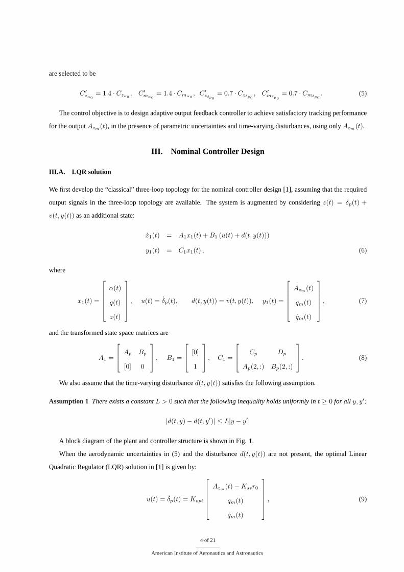
A block diagram of the plant and controller structure is shown in Fig. 1.

When the aerodynamic uncertainties in (5) and the disturbanced(t, y(t)) are not present, the optimal Linear

Quadratic Regulator (LQR) solution in [1] is given by:

u(t) = δp(t) = Kopt

Azm(t)−Kssr0

qm(t)

qm(t)

, (9)

4 of 21


),( pp BA pxpC

py

s

1 vp +δ

pD

d

uoptK

ssK~

zcA

Figure 1. Block diagram of system.

whereKss is chosen to ensure zero steady-state error for step commands, whiler0 is the steady-state value of the

reference commandr(t). Based on the nominal numerical values given in Table 1, the optimal controller gains are:

Kopt = [−1.3028 11.7544 0.3277], Kss = 1.0855.

In the current setup,qm(t) is not measurable, and the above computed optimal controller is actually the derivative

of δp(t). Since we have a linear system, we can integrate both sides of (9) to determineδp(t) (assuming constant

gains) as:

δp(t) = Kopt

∫ t

0(Azm(τ)−Kssr0) dτ

∫ t

0qm(τ)dτ

∫ t

0qm(τ)dτ

= Kopt

∫ t

0(Azm(τ)−Kssr0) dτ

∫ t

0qm(τ)dτ

qm(t)

. (10)

If the available feedback signal is onlyAzm , the above optimal controller cannot be implemented. The proposed

adaptive control method can have satisfactory tracking performance in the presence of parametric uncertainties and

disturbance, using onlyAzm as feedback signal. For comparison purposes, we design an observer that can recover

the original LQR control performance. At the same time we need to recover the inherent robustness of baseline LQR

controller as much as possible, because we are looking into the controller’s robustness to parametric uncertainties and

disturbance.

III.B. Output feedback solution: LQG/LTR

Based on the LQR solution of the above nominal optimal control, we can design a Linear Quadratic Gaussian (LQG)

with Loop Transfer Recovery (LTR) controller using only the outputAzm . Since the LQR controller is ready, we only

need to design the Kalman filter which can help recover the robustness of LQR controller. We note that due to the

non-minimum phase property of the system, the robustness recovery is limited.

In Mracek and Ridgely [1], the LQR design is based on the transformed system with state transformationx2 =

C1x1, as shown below

x2(t) = A2x2(t) + B2u(t)

y2(t) = x2(t) (11)

5 of 21


where

x2(t) =

Azm(t)

qm(t)

qm(t)

, A2 = C1A1C−11 , B2 = C1B1.

We design a Kalman filter based on this LQR solution. Plant noise and measurement noise are introduced to produce

x2(t) = A2x2(t) + B2u(t) + B2ω(t)

yk(t) = Azm(t) = [1 0 0]x2(t) + v(t) (12)

where the plant noiseω(t) and the measurement noisev(t) are white noises with the spectral densitiesSω andSv

respectively, and they are uncorrelated and orthogonal. Furthermore, the plant noise and the initial states of the system

(12) are assumed to be uncorrelated and orthogonal; so are the measurement noise and the states. The Kalman filter

equation is

˙x2(t) = A2x2(t) + B2u(t) + G (yk(t)− [1 0 0]x2(t)) (13)

whereG is the Kalman gain. The Loop Transfer Recovery design is done by increasing the spectral densitySω of

the plant noiseω(t). We choose different values ofSω to design the Kalman filter, and compare the results to the

LQR results. The spectral density of the measurement noise is set asSv = 0.1. The Kalman filter gain is obtained by

MATLAB command “kalman”. Next we show the system response of LQG/LTR control.

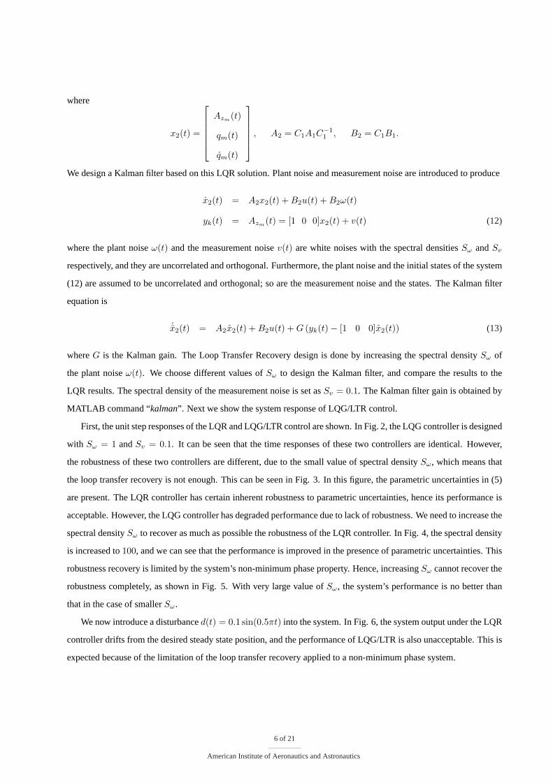
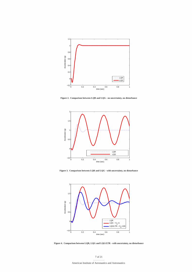
First, the unit step responses of the LQR and LQG/LTR control are shown. In Fig. 2, the LQG controller is designed

with Sω = 1 andSv = 0.1. It can be seen that the time responses of these two controllers are identical. However,

the robustness of these two controllers are different, due to the small value of spectral densitySω, which means that

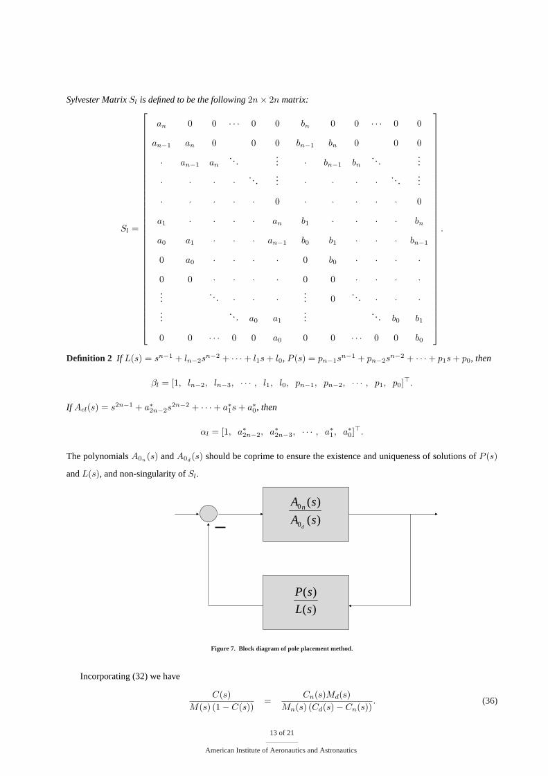
the loop transfer recovery is not enough. This can be seen in Fig. 3. In this figure, the parametric uncertainties in (5)

are present. The LQR controller has certain inherent robustness to parametric uncertainties, hence its performance is

acceptable. However, the LQG controller has degraded performance due to lack of robustness. We need to increase the

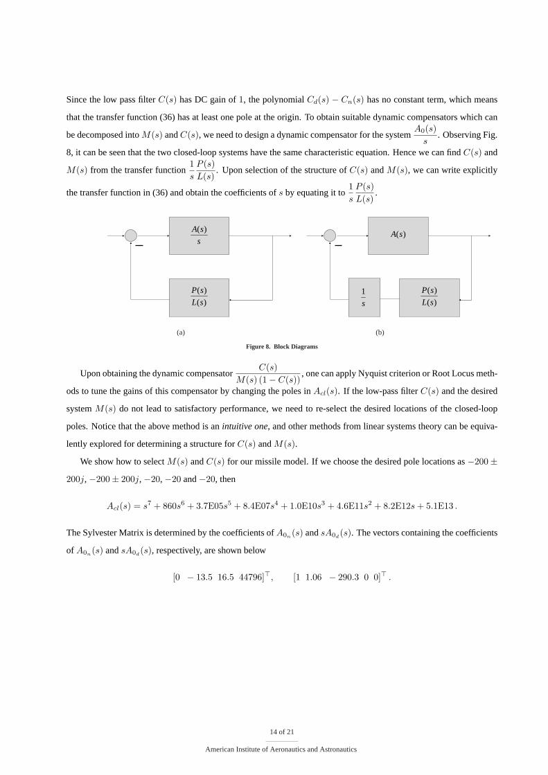
spectral densitySω to recover as much as possible the robustness of the LQR controller. In Fig. 4, the spectral density

is increased to100, and we can see that the performance is improved in the presence of parametric uncertainties. This

robustness recovery is limited by the system’s non-minimum phase property. Hence, increasingSω cannot recover the

robustness completely, as shown in Fig. 5. With very large value ofSω, the system’s performance is no better than

that in the case of smallerSω.

We now introduce a disturbanced(t) = 0.1 sin(0.5πt) into the system. In Fig. 6, the system output under the LQR

controller drifts from the desired steady state position, and the performance of LQG/LTR is also unacceptable. This is

expected because of the limitation of the loop transfer recovery applied to a non-minimum phase system.

6 of 21


0 0.2 0.4 0.6 0.8 1−0.2

0

0.2

0.4

0.6

0.8

1

1.2

time (sec)

Acc

eler

atio

n (g

)

LQRLQG

Figure 2. Comparison between LQR and LQG - no uncertainty, no disturbance

0 0.2 0.4 0.6 0.8 1−0.5

0

0.5

1

1.5

2

time (sec)

Acc

eler

aton

(g)

LQRLQG

Figure 3. Comparison between LQR and LQG - with uncertainty, no disturbance

0 0.2 0.4 0.6 0.8 1−0.5

0

0.5

1

1.5

2

time (sec)

Acc

eler

atio

n (g

)

LQR LQG − Sω=1

LQG/LTR − Sω=100

Figure 4. Comparison between LQR, LQG and LQG/LTR - with uncertainty, no disturbance

7 of 21


0 0.2 0.4 0.6 0.8 1−0.2

0

0.2

0.4

0.6

0.8

1

1.2

1.4

1.6

time (sec)

Acc

eler

atio

n (g

)

LQG/LTR − Sω=100

LQG/LTR − Sω=10000

LQG/LTR − Sω=1000000

Figure 5. Different values ofSω for LQG/LTR designs - with uncertainties, no disturbance

0 0.2 0.4 0.6 0.8 1−0.5

0

0.5

1

1.5

2

2.5

3

time (sec)

Acc

eler

aton

(g)

LQRLQG − Sω=1

LQG/LTR − Sω=100

Figure 6. Comparison between LQR, LQG and LQG/LTR - with uncertainties and disturbance

8 of 21


IV. L1 Adaptive Output Feedback Control

In system (6), if we lety(t) = C1(1, :)x1(t) = c>x1(t) = Azm(t), the longitudinal dynamics of the missile can

be presented in the following form:

y(s) = A(s) [u(s) + d(s)] , y(0) = 0 , (14)

whereu(t) = δp(t) ∈ R is the input,y(t) = Azm(t) ∈ R is the system output,A(s) = c>(sI − A1)−1B1 is the

unknown transfer function of the system,d(s) is the Laplace transform of the time-varying disturbances in (6). Notice

thatd(t, y) depends on the system outputy, and the upper bound of the growth rate ofd(t, y) with respect toy is L,

as stated in Assumption 1.

Substituting the numerical values from Table 1 into the system in (6), we get the nominal system ofA(s)

A0(s) =A0n

A0d

=−13.51s2 + 16.46s + 44800

s3 + 1.064s2 − 290.3s. (15)

To achieve the control objective, we need to design an adaptive output feedback controlleru(t) such that in the

presence of uncertainties the system outputy(t) tracks the reference inputr(t) with satisfactory performance. This can

be done by selecting a minimum-phase, strictly proper and stable transfer functionM(s), and designing an adaptive

control law to achievey(s) ≈ M(s)r(s). The selection ofM(s) needs to satisfy the sufficient conditions for stability

and performance, and we postpone the discussion on selection ofM(s) to Section V. The system in (14) can be

rewritten as:

y(s) = M(s) (u(s) + σ(s)) (16)

σ(s) =((A(s)−M(s))u(s) + A(s)d(s)

)/M(s) . (17)

Let (Am ∈ RN×N , bm ∈ RN , cm ∈ RN ) be the minimal realization ofM(s). Hence,(Am, bm, cm) is controllable

and observable, withAm being Hurwitz. Thus, the system in (16) can be rewritten as:

x(t) = Amx(t) + bm(u(t) + σ(t)) (18)

y(t) = c>mx(t) , x(0) = x0 = 0.

Next we introduce the closed-loopreference systemthat definesan achievable control objectivefor theL1 adaptive

controller.

Closed-loop reference system:The reference system is given by

yref (s) = M(s)(uref (s) + σref (s)) (19)

σref (s) =((A(s)−M(s))uref (s) + A(s)dref (s)

)/M(s)

uref (s) = C(s)(r(s)− σref (s))

whereC(s) is a low pass filter with DC gainC(0) = 1.

9 of 21


According to [2, Lemma 1] the selection ofC(s) andM(s) must ensure that

H(s) = A(s)M(s)/(C(s)A(s) + (1− C(s))M(s)

)(20)

is stable and that theL1-gain of the cascaded system is upper bounded as follows:

‖H(s)(1− C(s))‖L1L < 1 (21)

Then the reference system in (19) is stable.

The elements of theL1 adaptive controller are introduced next.

State predictor (passive identifier):Let (Am ∈ Rn×n, bm ∈ Rn, cm ∈ Rn ) be the minimal realization ofM(s).

Hence, (Am, bm, cm) is controllable and observable withAm being Hurwitz. Then the system in (14) can be rewritten

as

x(t) = Amx(t) + bm(u(t) + σ(t)) (22)

y(t) = c>mx(t)

The state predictor is given by:

˙x(t) = Amx(t) + bmu(t) + σ(t) (23)

y(t) = c>mx(t)

whereσ(t) ∈ Rn is the vector of adaptive parameters. Notice that in the state predictor equationsσ(t) is not in the

span ofbm, while in the equation (22)σ(t) is in the span ofbm. Further, lety(t) = y(t)− y(t).

Adaptation law: Let P be the solution of the following algebraic Lyapunov equation:

A>mP + PAm = −Q

whereQ > 0. From the properties ofP it follows that there always exists a nonsingular√

P such that

P =√

P>√

P .

Given the vectorc>m(√

P )−1, let D be the(n− 1)× n-dimensional nullspace ofc>m(√

P )−1, i.e.

D(c>m(√

P )−1)> = 0 (24)

and let

Λ =

c>m

D√

P

∈ Rn×n (25)

The update law forσ(t) is defined via the sampling timeT > 0a:

σ(iT ) = −Φ−1(T )µ(iT ), i = 1, 2, · · · , (26)

aT defines the sampling rate of the available CPU.

10 of 21


where

Φ(T ) =∫ T

0

eΛAmΛ−1(T−τ)Λdτ (27)

and

µ(iT ) = eΛAmΛ−1T 11y(iT ), i = 1, 2, · · · (28)

Here11 denotes the basis vector in the spaceRn with its first element equal to1 and other elements being zero.

Control law: The control law is defined via the output of the low-pass filter:

u(s) = C(s)r(s)− C(s)M(s)

c>m(sI−Am)−1σ(s) . (29)

The completeL1 adaptive controller consists of the state predictor in (23), the adaptation law in (26), and the

control law in (29), subject to theL1-gain upper bound in (21). The performance bounds of theL1 adaptive output

feedback controller are given by the following theorem.

Theorem 1

limT→0

(‖y‖L∞)

= 0

limT→0

(‖y − yref‖L∞)

= 0

limT→0

(‖u− uref‖L∞)

= 0

The result in this theorem follows immediately from [2, Theorem 1] and [2, Lemma 3].

V. Design Issues ofL1 Adaptive Output Feedback Control

V.A. Stability

The first step of designing anL1 adaptive output feedback controller is to guarantee stability of the closed-loop system.

From Theorem 1 it can be seen that the output of the closed-loop system tracks that of the closed-loop reference system

arbitrarily closely for allt > 0. Hence the goal of the first step in the design is to findC(s) andM(s) to satisfy the

sufficient conditions given in (20) and (21). These two conditions can guarantee the stability of closed-loop reference

system.

We first discuss the classes of systems that can satisfy (20) via the choice ofM(s) andC(s). We demonstrate that

stability ofH(s) is equivalent to stabilization ofA(s) by

C(s)M(s)(1− C(s))

. (30)

Consider the closed-loop system, comprised of the systemA(s) and negative feedback of (30). The closed-loop

transfer function is:A(s)

1 + A(s) C(s)M(s)(1−C(s))

. (31)

11 of 21


Letting

A(s) =An(s)Ad(s)

, C(s) =Cn(s)Cd(s)

, M(s) =Mn(s)Md(s)

, (32)

it follows from (20) that

H(s) =Cd(s)Mn(s)An(s)

Hd(s), (33)

where

Hd(s) = Cn(s)An(s)Md(s) + Mn(s)Ad(s)(Cd(s)− Cn(s)). (34)

Incorporating (32), one can verify that the denominator of the system in (31) is exactlyHd(s). Hence, stability of

H(s) is equivalent to the stability of the closed-loop system in (31).

The selection ofM(s) andC(s) can be restricted due to the properties of the plantA(s). Thus, it is not a trivial

task. However, it can be done using linear systems theory. The essential objective in this step is to design, based on the

nominal systemA0(s), a feedback controller that can be decomposed intoC(s) andM(s) according to the equation

(30), while achieving stability ofH(s) in (20) and verifying the condition in (21) based on conservative knowledge of

parametric variations inA(s). In the following subsection we describe one method towards the selection ofC(s) and

M(s).

V.A.1. Design via pole placement

We use a pole placement method (see examples in Ioannou and Sun [5]) to design a dynamic compensator forA0(s).

The block diagram in Fig. 7 shows the structure of the closed-loop system, where the dynamic controllerP (s)/L(s)

is determined by the solution of the following equation

A0n(s)P (s) + A0d(s)L(s) = Acl(s). (35)

All terms in (35) are polynomials ofs. The Hurwitz polynomialAcl(s) defines the desired pole locations of the closed-

loop system. The coefficients of polynomialsP (s) andL(s) may be obtained by solving the algebraic equation

βl = Sl−1αl

containing the Sylvester matrixSl of A0n andA0d, whileβl is a vector containing coefficients of bothP (s) andL(s),

andαl is a vector containing coefficients ofAcl(s) (defined next).

Definition 1 Given two polynomialsa(s) = ansn + an−1sn−1 + · · ·+ a0, b(s) = bnsn + bn−1s

n−1 + · · ·+ b0, the

12 of 21


Sylvester MatrixSl is defined to be the following2n× 2n matrix:

Sl =

an 0 0 · · · 0 0 bn 0 0 · · · 0 0

an−1 an 0 0 0 bn−1 bn 0 0 0

· an−1 an.. .

... · bn−1 bn. ..

...

· · · · . . .... · · · · . . .

...

· · · · · 0 · · · · · 0

a1 · · · · an b1 · · · · bn

a0 a1 · · · an−1 b0 b1 · · · bn−1

0 a0 · · · · 0 b0 · · · ·0 0 · · · · 0 0 · · · ·...

.. . · · · ... 0. .. · · ·

..... . a0 a1

.... .. b0 b1

0 0 · · · 0 0 a0 0 0 · · · 0 0 b0

.

Definition 2 If L(s) = sn−1 + ln−2sn−2 + · · ·+ l1s + l0, P (s) = pn−1s

n−1 + pn−2sn−2 + · · ·+ p1s + p0, then

βl = [1, ln−2, ln−3, · · · , l1, l0, pn−1, pn−2, · · · , p1, p0]>.

If Acl(s) = s2n−1 + a∗2n−2s2n−2 + · · ·+ a∗1s + a∗0, then

αl = [1, a∗2n−2, a∗2n−3, · · · , a∗1, a∗0]>.

The polynomialsA0n(s) andA0d(s) should be coprime to ensure the existence and uniqueness of solutions ofP (s)

andL(s), and non-singularity ofSl.

)(

)(

0

0

sA

sA

d

n

)(

)(

sL

sP

Figure 7. Block diagram of pole placement method.

Incorporating (32) we have

C(s)M(s) (1− C(s))

=Cn(s)Md(s)

Mn(s) (Cd(s)− Cn(s)). (36)

13 of 21


Since the low pass filterC(s) has DC gain of1, the polynomialCd(s) − Cn(s) has no constant term, which means

that the transfer function (36) has at least one pole at the origin. To obtain suitable dynamic compensators which can

be decomposed intoM(s) andC(s), we need to design a dynamic compensator for the systemA0(s)

s. Observing Fig.

8, it can be seen that the two closed-loop systems have the same characteristic equation. Hence we can findC(s) and

M(s) from the transfer function1s

P (s)L(s)

. Upon selection of the structure ofC(s) andM(s), we can write explicitly

the transfer function in (36) and obtain the coefficients ofs by equating it to1s

P (s)L(s)

.

s

sA )(

)(

)(

sL

sP

(a)

)(sA

)(

)(

sL

sP

s

1

(b)

Figure 8. Block Diagrams

Upon obtaining the dynamic compensatorC(s)

M(s) (1− C(s)), one can apply Nyquist criterion or Root Locus meth-

ods to tune the gains of this compensator by changing the poles inAcl(s). If the low-pass filterC(s) and the desired

systemM(s) do not lead to satisfactory performance, we need to re-select the desired locations of the closed-loop

poles. Notice that the above method is anintuitive one, and other methods from linear systems theory can be equiva-

lently explored for determining a structure forC(s) andM(s).

We show how to selectM(s) andC(s) for our missile model. If we choose the desired pole locations as−200±200j,−200± 200j,−20,−20 and−20, then

Acl(s) = s7 + 860s6 + 3.7E05s5 + 8.4E07s4 + 1.0E10s3 + 4.6E11s2 + 8.2E12s + 5.1E13 .

The Sylvester Matrix is determined by the coefficients ofA0n(s) andsA0d(s). The vectors containing the coefficients

of A0n(s) andsA0d(s), respectively, are shown below

[0 − 13.5 16.5 44796]>, [1 1.06 − 290.3 0 0]> .

14 of 21


The Sylvester MatrixSl is

Sl =

1 0 0 0 0 0 0 0

1.06 1 0 0 0 0 0 0

−290.3 1.06 1 0 −13.5 0 0 0

0 −290.3 1.06 1 16.5 −13.5 0 0

0 0 −290.3 1.06 44796 16.5 −13.5 0

0 0 0 −290.3 0 44796 16.5 −13.5

0 0 0 0 0 0 44796 16.5

0 0 0 0 0 0 0 44796

We solve the following algebraic equation

βl = Sl−1αl

to get the vectorβl:

βl = [1 858 4.6E06 2.4E08 3.1E05 1.2E07 1.8E08 1.1E09]> ,

whereαl is the vector of the coefficients ofAcl(s).

The first four elements ofβl are the coefficients ofL(s), and the rest of the elements are the coefficients ofP (s).

Hence,

L(s) = s3 + 858s2 + 4.6E06s + 2.4E08,

P (s) = 3.1E05s3 + 1.2E07s2 + 1.8E08s + 1.1E09.

If we selectC(s) to be a second order, relative degree2 transfer function, andM(s) be third order, relative degree1

transfer function, we can write explicitly the transfer function in (36) and obtain the coefficients ofM(s) andC(s) by

equating (36) to1s

P (s)L(s)

. The transfer functions forC(s) andM(s) take the form:

M(s) =s2 + 806s + 4.5E06

s3 + 39.02s2 + 585s + 3665, (37)

C(s) =3.1E05

s2 + 52.61s + 3.1E05. (38)

This selection ofM(s) andC(s) generate satisfactory performance according to simulation results shown in Section

VI.

V.A.2. Stability check

We notice that the design of the dynamic compensator is based on our knowledge of the nominal plantA0(s). We

know the bounds for the variation of the system parameters, but not the exact values of these parameters. The stability

15 of 21


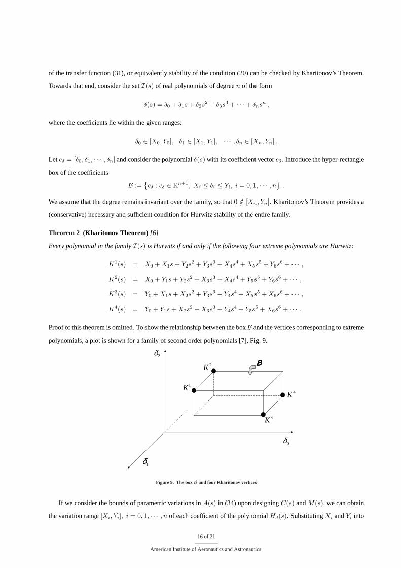
of the transfer function (31), or equivalently stability of the condition (20) can be checked by Kharitonov’s Theorem.

Towards that end, consider the setI(s) of real polynomials of degreen of the form

δ(s) = δ0 + δ1s + δ2s2 + δ3s

3 + · · ·+ δnsn ,

where the coefficients lie within the given ranges:

δ0 ∈ [X0, Y0], δ1 ∈ [X1, Y1], · · · , δn ∈ [Xn, Yn] .

Let cδ = [δ0, δ1, · · · , δn] and consider the polynomialδ(s) with its coefficient vectorcδ. Introduce the hyper-rectangle

box of the coefficients

B :={cδ : cδ ∈ Rn+1, Xi ≤ δi ≤ Yi, i = 0, 1, · · · , n

}.

We assume that the degree remains invariant over the family, so that0 /∈ [Xn, Yn]. Kharitonov’s Theorem provides a

(conservative) necessary and sufficient condition for Hurwitz stability of the entire family.

Theorem 2 (Kharitonov Theorem) [6]

Every polynomial in the familyI(s) is Hurwitz if and only if the following four extreme polynomials are Hurwitz:

K1(s) = X0 + X1s + Y2s2 + Y3s

3 + X4s4 + X5s

5 + Y6s6 + · · · ,

K2(s) = X0 + Y1s + Y2s2 + X3s

3 + X4s4 + Y5s

5 + Y6s6 + · · · ,

K3(s) = Y0 + X1s + X2s2 + Y3s

3 + Y4s4 + X5s

5 + X6s6 + · · · ,

K4(s) = Y0 + Y1s + X2s2 + X3s

3 + Y4s4 + Y5s

5 + X6s6 + · · · .

Proof of this theorem is omitted. To show the relationship between the boxB and the vertices corresponding to extreme

polynomials, a plot is shown for a family of second order polynomials [7], Fig. 9.

0δ

1δ

2δ2K

1K

3K

4K

ΒΒΒΒ

Figure 9. The boxB and four Kharitonov vertices

If we consider the bounds of parametric variations inA(s) in (34) upon designingC(s) andM(s), we can obtain

the variation range[Xi, Yi], i = 0, 1, · · · , n of each coefficient of the polynomialHd(s). SubstitutingXi andYi into

16 of 21


the four extreme polynomials, we only need to check the stability of these four polynomials. If these four polynomials

are stable, the designedC(s) andM(s) are acceptable for verification of the condition in (20).

Upon the design of transfer functionsC(s) andM(s), the condition (21) needs to be checked. This follows from

the same procedure of the results in Cao and Hovakimyan [8,9].

V.B. Performance

The second step is to ensure satisfactory performance. Upon determining the structure ofM(s) andC(s), which

can satisfy the sufficient conditions for stability, we can tune the parameters ofM(s) andC(s) within the acceptable

parameter space to achieve satisfactory performance. The tuning of parameters forM(s) follows from conventional

linear systems theory, which we omit here. The guideline for tuning the low-pass filterC(s) follows the same lines

of Cao and Hovakimyan [8, 9]. The trade-off between the time-delay margin and the performance of theL1 adaptive

controller depends solely uponC(s). Increasing the bandwidth ofC(s) leads to improved performance at the price of

reduced time-delay margin. In [10], we consider constrained optimization of the performance and/or the robustness of

L1 adaptive controller by resorting to appropriate Linear Matrix Inequality (LMI) type conditions. If the corresponding

LMI has a solution, then arbitrary desired performance bound can be achieved, while retaining a prespecified lower-

bound on the time-delay margin.

In summary, to gain more freedom in design, it is important for designers to find the largest possible acceptable

parameter space in the first step discussed in section V.A.

VI. Simulation Example

The nominal transfer function of the unstable non-minimum phase missile plant in (15) is repeated below:

A(s) =−13.51s2 + 16.46s + 44800

s3 + 1.064s2 − 290.3s, (39)

and the desired systemM(s) and the low-pass filterC(s) are taken from (37) and (38):

M(s) =s2 + 806s + 4.5E06

s3 + 39.02s2 + 585s + 3665, (40)

C(s) =3.1E05

s2 + 52.61s + 3.1E05. (41)

We selectT = 0.0001. TheL1 output feedback adaptive control approach is applied to this system. Fig. 10 shows

the system outputs withL1 controller, in the absence and in the presence of parametric uncertainties. We can see that

the system output tracks the step command satisfactorily. Although this response is different from that of the baseline

LQR controller, we demonstrate later that in different unknown scenarios, theL1 controlled system still has a uniform

response close to the one shown in Fig. 10, independent of the nature of the uncertainty. This verifies the theoretical

claim on uniform approximation of the corresponding signals of a bounded reference system. In Fig. 11 the control

signal is shown, which is guaranteed to stay in low frequency range.

17 of 21


The disturbance is then introduced, as shown in Fig. 12. Sinced(t) does not depend on the system outputy(t),

the condition in (21) is satisfied automatically. We see that the output response is slightly different than that of the

nominalL1 case, but is still satisfactory. To explain this, we look into the closed loop reference system (19). It can be

shown that

yref (s) = M(s) [C(s)r(s) + (1− C(s))σref (s)]

= M(s)[C(s)r(s) +

C(s)(1− C(s))(A(s)−M(s))M(s) + (A(s)−M(s))C(s)

r(s) +(1− C(s))A(s)

M(s) + (A(s)−M(s))C(s)d(s)

].

The transfer function fromd(s) to yref (s) can be expressed as

(Cd(s)− Cn(s))An(s)Mn(s)(Cd(s)− Cn(s))Ad(s)Mn(s) + An(s)Md(s)Cn(s)

. (42)

The magnitude curve of the Bode diagram is given in Fig. 13, which shows disturbance attenuation at low and high

frequencies. This behavior of the reference system can be improved by manipulating the bandwidths ofM(s) and

C(s). For our non-minimum phase, unstable systemA(s), the possible selections are not many.

0 0.2 0.4 0.6 0.8 1−0.2

0

0.2

0.4

0.6

0.8

1

1.2

time (sec)

Acc

eler

atio

n (g

)

L1 − no uncertainty no disturbance

L1 − with uncertainty, no disturbance

Figure 10. Closed loop response ofL1 controller - with/without uncertainties, no disturbance

Finally the parametric uncertainties are changed due to a change in aerodynamic coefficients given below:

C ′zα0= 1.2 · Czα0

, C ′mα0= 1.5 · Cmα0

, C ′zδp0= 0.8 · Czδp0

, C ′mδp0= 0.7 · Cmδp0

. (43)

The system output is shown in Fig. 14. We can see that theL1 output feedback adaptive control still has uniform

performance.

18 of 21


0 0.2 0.4 0.6 0.8 1−0.2

−0.15

−0.1

−0.05

0

0.05

0.1

0.15

time (sec)

δ p (ra

d)

L1 control signal − with uncertainty, no disturbance

Figure 11. Control signal ofL1 controller

0 0.2 0.4 0.6 0.8 1−0.2

0

0.2

0.4

0.6

0.8

1

1.2

time (sec)

Acc

eler

atio

n (g

)


L1 − with uncertainty and disturbance

Figure 12. Closed loop response ofL1 controller - with uncertainties and disturbance

10−1

100

101

102

103

104

105

−80

−70

−60

−50

−40

−30

−20

−10

0

10

Mag

nitu

de (

dB)

Bode Diagram

Frequency (rad/sec)

Figure 13. Frequency response of transfer function fromd to yref

19 of 21


0 0.2 0.4 0.6 0.8 1−0.2

0

0.2

0.4

0.6

0.8

1

1.2

time (sec)

Acc

eler

atio

n (g

)


L1 − with uncertainty case 2, and disturbance

Figure 14. Closed loop response ofL1 controller with different uncertainties

VII. Conclusion

Longitudinal autopilot design for a missile model is performed usingL1 adaptive output feedback controller,

appropriate for non-SPR reference system dynamics. The new piece-wise constant adaptive law along with the low-

pass filtered control signal ensures uniform performance bounds for system’s both input/output signals as compared

to the corresponding signals of a non-SPR reference system. The simulation responses of the proposed controller are

compared to those of baseline LQR and LQG/LTR design, and the benefits of theL1 adaptive controller are clearly

demonstrated.

VIII. Acknowledgment

This material is based upon work supported by the AFOSR under Contract FA9550-08-1-0135. Any opinions,

findings and conclusions or recommendations expressed in this material are those of the authors and do not necessarily

reflect the views of United States Air Force.

References

1C. P. Mracek and D. B. Ridgely, Missile Longitudinal Autopilots: Connections Between Optimal Control and Classical Topologies,Proceed-

ings of AIAA Guidance, Navigation, and Control Conference and Exhibit, San Francisco, CA, 2005.

2C. Cao and N. Hovakimyan,L1 Adaptive Output Feedback Controller for Systems of Unknown Relative Degree,Submitted to American

Control Conference, 2009.

3C. Cao and N. Hovakimyan,L1 Adaptive Output Feedback Controller for Non Strictly Positive Real Reference Systems,Submitted to

American Control Conference, 2009.

4C. Cao and N. Hovakimyan.L1 Adaptive Output Feedback Controller for Systems of Unknown Dimension.IEEE Transactions on Automatic

Control, 53:815–821, April 2008.

5P. A. Ioannou and J. Sun,Robust Adaptive Control. NJ, Prentice Hall, 1995.

20 of 21


6V. L. Kharitonov, Asymptotic Stability of an Equilibrium Position of a Family of Systems of Linear Differential Equations,Differential

Uravnen, 14:2086-2088, 1978.

7S. P. Bhattacharyya, H. Chapellat and L. H. Keel,Robust Control: The Parametric Approach. NJ, Prentice Hall, 1995.

8C. Cao and N. Hovakimyan, Design and Analysis of a NovelL1 Adaptive Control Architecture, Part I: Control Signal and Asymptotic

Stability, American Control Conference, pages 3397-3402, 2006.

9C. Cao and N. Hovakimyan, Design and Analysis of a NovelL1 Adaptive Control Architecture, Part II: Guaranteed Transient Performance,

American Control Conference, pages 3403-3408, 2006.

10D. Li, N. Hovakimyan, C. Cao and K. Wise, Filter Design for Feedback-loop Trade-off ofL1 Adaptive Controller: A Linear Matrix

Inequality Approach,Proceedings of AIAA Guidance, navigation and Control Conference, Honolulu, HI, August 2008.

21 of 21


l1 adaptive controller for a missile longitudinal ...ccao/caopaper/wangaiaa08l1.pdf · this paper...

Documents