l partial moments as a measure of vulnerability to poverty...

1

LOWER PARTIAL MOMENTS AS A MEASURE OF VULNERABILITY TO POVERTY IN CAMEROON

Rudolf Witt*, Hermann Waibel

Institute of Development and Agricultural Economics, Faculty of Economics and Management,

Leibniz Universität Hannover, Königsworther Platz 1, 30167 Hannover, Germany

Discussion Paper No. 434

November 2009 Abstract

In this paper the class of Lower Partial Moments (LPMs) is used for measuring vulnerability

as downside risk of household income in rural Cameroon. This class of established and

coherent risk measures has been shown to meet a number of desirable properties. Among

others, the LPMs fulfill the focus axiom, and for order greater than zero they are in harmony

with expected utility theory under the weak assumption of risk aversion. Through

combining the vulnerability measure with a portfolio approach it is possible to distinguish

different livelihood systems for which the poverty and vulnerability measures are the

explicit result of stochastic distributions of single activities in the households’ portfolio and

their covariance structure. In particular we consider the four major income generating

activities in the study area: Sorghum, millet and rice production, and fishing. The results

suggest that in the study area fishermen are less affected by adverse effects on income than

other livelihood systems, while rice growers are the poorest and most vulnerable. It is also

shown that rice and millet growers are suffering from chronic poverty, while transient

poverty is more prevalent among the group of sorghum growers and fishermen. This

implication is further confirmed by assuming a moving target equal to the mean portfolio

income for the calculation of LPMs. The results of the scenario analysis suggest that policy

interventions aiming at a reduction of the covariation structure between income flows from

different activities are quite promising.

Keywords: Vulnerability as expected poverty, Lower Partial Moments, portfolio theory,

diversification, Sub Saharan Africa

JEL Classification: I32, O13, G11, G32

*corresponding author: e-mail: [email protected]; tel.: +49-511-762-5414

2

Introduction

Research on poverty has more and more acknowledged that uncertainty and risk need to be

considered in measuring the welfare position of households. In particular, the concept of

vulnerability has recently become quite prominent in theoretical and empirical research.

Inspired by Ravallion (1988), vulnerability is mostly defined as expected poverty (VEP).

Methodologically, VEP measures extend the static Foster‐Greer‐Thorbecke (FGT) poverty

measures to make predictions on the probability of being poor in the future. Some examples

of this approach can be found in Pritchett et al. (2000), Chaudhuri et al. (2002), Christiansen

and Subbarao (2005), Kamanou and Morduch (2001), Günther and Hattgen (2006, 2009),

Günther and Maier (2008), Béné (2009), and Chiwaula et al. (2009).

Although some authors (e.g. Ligon and Schechter 2003, Calvo and Dercon 2005) have been

arguing that the VEP measure seems to be ill‐suited to represent household risk attitudes, it

fulfills many desirable properties which are also inherent to the FGT poverty measures,

including symmetry, replication invariance, subgroup consistency and decomposability

(Foster et al. 1984). In particular, the VEP is fulfilling the focus axiom, which states that

vulnerability measures should focus on downside risk only, since favorable outcomes in

good states of the world do not necessarily ensure lower vulnerability (Calvo and Dercon

2005).

To address the critique of implicit risk attitude assumptions of the VEP, we suggest that the

general concept of vulnerability, defined as an ex‐ante risk measure based on stochastic

welfare distributions, is not different from risk analysis concepts as they have been widely

applied in the finance world since the 1950s, for example to pricing, hedging, portfolio

optimization or capital allocation. In particular, we propose the use of the Lower Partial

Moments (LPMs) as a measure of vulnerability as expected poverty. Without explicitly

referring to the LPMs, this approach has also been applied in a slightly modified

specification by Christiaensen and Subbarao (2005). The LPMs are one class of coherent

measures of risk, introduced by Fishburn (1977) and Bawa (1975, 1978), which are measures

of downside or shortfall risk, where only negative deviations from a target outcome are

taken into consideration. In contrast to symmetrical risk measures, the LPMs capture the

3

common notion of risk as a negative, undesired characteristic of an alternative (Brogan and

Stidham 2005, Albrecht and Maurer 2002, Unser 2000), which is also in line with the focus

axiom. Further, LPMs have a number of convenient characteristics. First, they are consistent

to the ordering of distributions derived from stochastic dominance rules and utility

maximization for risk‐averse households. Second, LPMs are coherent risk measures,

satisfying the axioms of subadditivity, positive homogeneity, monotonicity and translation

invariance (Artzner et al. 1999, Cheng et al. 2004, Acerbi et al. 2001, Acerbi and Tasche 2002,

Peracci and Tanase 2008). This set of axioms has been widely accepted and regarded as a

landmark in the field of risk theory (Cheng et al. 2004). Third, analogous to the FGT

measures, the LPMs are additively decomposable, so that vulnerability can be measured not

only on individual or household level, but also be aggregated for different population

groups. And finally, LPMs are intuitively interpretable, an attribute that is of eminent

importance in view of policy advise. Analogous to the class of FGT poverty indicators, the

LPMs not only identify the vulnerable, but also show how pronounced vulnerability is in

terms of consumption or income under downside risk.

A related question that we also address here is, how to derive a stochastic distribution of

welfare, particularly income. This issue is critical for vulnerability assessment, since

vulnerability measures are always based on the estimated mean and variance of a welfare

indicator. However, panel data of sufficient length are virtually not existing for most

developing countries. Thus, some authors have suggested to apply econometric models such

as the 3‐step FGLS model (Just and Pope 1979), which assumes that intertemporal variation

is reflected in the cross‐sectional variation of the error term. A possible alternative presented

here is a simple risk assessment method, which is fully sufficient do derive an outcome‐

activity matrix as suggested by portfolio theory (Witt and Waibel 2009).

This paper is organized as follows: In the next section we will briefly outline the portfolio

theory which is used to calculate stochastic income distribution parameters, and also

introduce the LPM risk measure and discuss its properties. The remaining part of the paper

presents an empirical application on data from 238 rural households in Northern Cameroon

in 2008. We close with a short conclusion and suggestions for further research.

4

Portfolio theory and LPMs

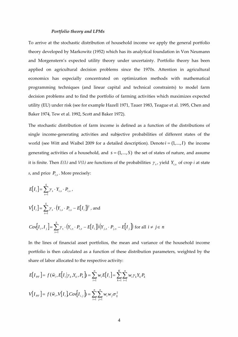
To arrive at the stochastic distribution of household income we apply the general portfolio

theory developed by Markowitz (1952) which has its analytical foundation in Von Neumann

and Morgenstern’s expected utility theory under uncertainty. Portfolio theory has been

applied on agricultural decision problems since the 1970s. Attention in agricultural

economics has especially concentrated on optimization methods with mathematical

programming techniques (and linear capital and technical constraints) to model farm

decision problems and to find the portfolio of farming activities which maximizes expected

utility (EU) under risk (see for example Hazell 1971, Tauer 1983, Teague et al. 1995, Chen and

Baker 1974, Tew et al. 1992, Scott and Baker 1972).

The stochastic distribution of farm income is defined as a function of the distributions of

single income‐generating activities and subjective probabilities of different states of the

world (see Witt and Waibel 2009 for a detailed description). Denote )...,,1( Ii = the income

generating activities of a household, and )...,,1( Ss = the set of states of nature, and assume

it is finite. Then E(Ii) and V(Ii) are functions of the probabilities sγ , yield siY , of crop i at state

s, and price siP , . More precisely:

[ ] ∑=

⋅⋅=S

ssisisi PYIE

1,,γ ,

[ ] [ ]( )∑=

−⋅⋅=S

sisisisi IEPYIV

1

2,,γ , and

[ ] [ ]( ) [ ]( )jsjsj

S

sisisisji IEPYIEPYIICov −⋅⋅−⋅⋅= ∑

=,,

1,,, γ for all nji ∈≠

In the lines of financial asset portfolios, the mean and variance of the household income

portfolio is then calculated as a function of these distribution parameters, weighted by the

share of labor allocated to the respective activity:

[ ] [ ] [ ] ∑∑∑= ==

===K

k

n

ikkki

n

iiikkkiiPF PYwIEwPYIEwfIE

1 11),,,( γγr

[ ] [ ] [ ] ∑∑= =

==n

i

n

jijjijiiiPF wwICovIVwfIV

1 1

2, ),,( σr

5

Thus, the two moments of the distribution of portfolio income describe the stochastic nature

of production, depending on the uncertain outcomes of the single activities, and the

covariance structure.

Departing from the early portfolio models which were simply based on variance (or

standard deviation) as risk measure, it has been argued that the variance of an outcome

variable is a dubious measure of risk, since making decisions on production or investment in

a risky environment is mostly concerned with expected losses rather than expected gains.

Due to the symmetrical nature of variance, this measure assigns the same weight to positive

as to negative deviations from the expected value and hence does not capture the common

notion of risk as a negative, undesired characteristic of an alternative, nor does it account for

fat tails of the underlying distribution (Cheng et al 2004, Jarrow and Zhao 2006, Brogan and

Stidham 2008, Albrecht and Maurer 2002, Unser 2000). An experimental study by Unser

(2000) shows that symmetrical risk measures can be clearly dismissed in favor of shortfall

measures like LPMs. Hence, some recent risk assessment approaches have been using Lower

Partial Moments (LPM) to describe investments in financial assets (for example Nawrocki

1999, Schubert and Bouza 2004, Ballestro et al. 2007). Qui et al. (2001), Liu et al. (2008) and

Webby et al. (2008) applied the framework of partial moments (upper partial moments or the

Conditional Value‐at‐Risk, which is a special case of the LPM measures) on agricultural

production decisions in an uncertain environment.

The Lower Partial Moment of the lth order is defined as:

[ ] ∫∞−

+ −=−=x

lll duufuxuxEuxLPM )()())((:),( , where x is a target separating gains and

losses, u is a random variable (e.g. income) and f(.) is a probability distribution function. The

reference point x can be specified as a fixed target, e.g. a given income poverty line which

applies to all households equally, or as a moving target, i.e. the target is not fixed but

depends on the household specific distribution of the random variable (Brogan and Stidham

2008). Schubert (1996) shows that for a normally distributed variable, the LPM of the lth

order can be computed as:

dueuxLPMux

ll

2

2

2)(

)(21 σ

μ

πσ

−−

∞−

⋅−= ∫

6

Setting l=0 yields the target shortfall probability1. The LPM of the order l=1 is the target

shortfall mean, often also called expected loss or expected shortfall. The LPM of order l=2 is

known as the target shortfall variance or target semi‐variance. In this case risk is measured

by squared deviations below the target x.

Applying LPMs as a measure of income risk is appealing in that there is no need to explicitly

assume an arbitrary risk aversion parameter since LPMs are consistent to the ordering of

distributions derived from stochastic dominance rules and utility maximization for risk‐

averse households (Bawa and Lindenberg 1977). Unser (2000) shows that for F to be

preferred to G it is necessary and sufficient that:

• For all { } FSDLPMLPMxuxuUxu GF ⇔≤=>′≡∈ ,0,01 :0)()()(

• For all { } SSDLPMLPMxuandxuxuUxu GF ⇔≤=<′′>′≡∈ ,1,12 :0)(0)()()(

• For all { } TSDLPMLPMxuandxuxuxuUxu GF ⇔≤=>′′′<′′>′≡∈ ,2,23 :0)(0)(;0)()()( .

Hence, the concerns raised concerning the implicit assumption of unrealistic risk attitudes by

VEP measures are invalid for the class LPMs. 1LPM is consistent with the HARA, and 2LPM

is consistent with the DARA class of utility functions (Persson 2000).

Given the assumption of normal distribution, LPMs can be easily computed by creating a

standardized variable σμ−

=xm , so that:

• )()(0 mxFLPM Φ==

• )()()(1 mmxLPM ϕσμ +Φ−=

• ( )[ ] )()()(222 mxmxLPM ϕμσσμ −+Φ+−= .

Analogous to the FGT poverty indicators, which are defined as α

α ∑=

⎟⎟⎠

⎞⎜⎜⎝

⎛ −=

N

i

i

zyz

NzP

1

*1)( ,

LPMs can be used to implement the risk dimension in measuring welfare (Table 1).

Table 1: Analogy between FGT and LPM indicators

1 The 0LPM is equivalent to the definition of vulnerability as the probability to be poor (e.g. Chaudhuri et al. 2002). Under the assumption of normal distribution, vulnerability is defined as:

⎥⎥⎦

⎤

⎢⎢⎣

⎡ −Φ=≤=

)(ˆ)(ˆ()Pr(

uV

uExxuvht .

7

FGT LPM Order Indicator Interpretation Order Indicator Interpretation

α=0 Poverty incidence Headcount ratio l=0

Shortfall probability

Probability that expected income will be lower than target

α=1 Poverty depth

Poverty Gap Index = average shortfall of living standards from the poverty line l=1

Expected Shortfall

Expected negative deviation from target

α=2 Poverty severity

Weighted sum of poverty gaps (e.g. Squared Poverty Gap Index)

l=2 Target Semi‐Variance

Squared deviations below the target.

Source: own illustration

Setting the target x equal to a given poverty line, FGT poverty measures and LPMs can be

directly compared. A potential problem with the safety‐first criterion is that the definition of

the subsistence minimum is essentially arbitrary (Alderman and Paxson 1992). The same

concern is also often raised regarding the use of a poverty line for general economic poverty

analysis. A possible solution is the use of a moving target [ ]uEx = (Brogan and Stidham

2008, Povell 2009). In the case of a normal distribution 0LPM would be 0.5 for all cases. The

1LPM however would reflect the risk of loss relative to the respective household’s living

standard and not to an arbitrary poverty line. It seems reasonable to assume that the overall

objective of an economic agent is to not fall below the expected or mean income, i.e. to

improve or at least to maintain the habitual living standard. The assumption of a poverty

line may do injustice to households that are relatively better off, but still face a high risk of

losses due to some stochastic events. Nonetheless, for the purpose of this paper we assume a

fixed income poverty line, which we define as 50% of the average portfolio income of the

sample. This assumption still permits to derive risk measures for all households irrespective

of their classification as poor or non‐poor applying the FGT measure.

Study site and data collection

The approach proposed here has been applied on data that were collected in the Logone

floodplain in the Far‐North province of Cameroon in May 2008. Ecologically, this area is

characterized by Sudano‐Sahelian climate and vegetation. The livelihoods of the people

8

living in this area (mainly subsistence agriculture and small‐scale fisheries) are heavily

dependent on natural resources and climate conditions. Due to the increasing aridification

and increased frequency of droughts and floods, agricultural production in this area has

been shifting to hardy plants with relatively low water requirements and a short growing

season, such as sorghum and millet. Fishing is a major activity for many households in terms

of nutrient supply and income generation and is carried out by almost every conceivable

means.

A two‐step weighted random sampling procedure was employed to identify the sample

households. Data were collected in May 2008. The final sample size after data entry and

cleaning is 238 households.

For the collection of data on crop yields, prices, and income flows from fishing, we applied a

visual impact method (VIM), based on Hardacker et al. (1997). VIM is an approach to elicit

subjective probabilities for stochastic outcomes, as long as the number of possible outcomes

is not too great. In our case we delimited the states of the world to S=3, i.e. “bad year”,

“normal year” and “good year”. In a risk assessment interview, three rectangles were drawn

on the soil, designating the three states of the world. After enquiring about the household’s

main income generating activity, each respondent (usually the household head) was then

asked to report how often out of the past ten years (covering the period 1998‐2008) they had

encountered a bad, normal or good year in this primary activity. For this exercise they were

given 10 stones and asked to allocate them among the three rectangles. The relative number

of stones in each state of the world represents the subjective probability of facing a certain

climatic event (either normal, adverse or favorable). Referring to this probability distribution,

several questions followed concerning the average yield levels for the primary crop (as well

as for all complementary activities carried out by the household) in each state of the world.

The data that was generated through this exercise was used to derive probability density

functions for each activity, as well as the correlation coefficients between the activities.

A limitation of this approach is that it is not possible to cover the tails of the yield

distributions for complementary activities, since the primary activity is taken as a reference.

However, in the presence of data limitations this constraint had to be accepted for the benefit

of capturing the correlation structure between different activities.

9

The labor input data that was used for portfolio analysis has been reported in mandays for

the year 2007, covering all seasons. This data has been used as an approximation for the

average labor input.

Results

Overall, the results show similar behavior of the poverty (FGT) and vulnerability (LPM)

measures, which is in line with the majority of research findings. Vulnerability is nonetheless

found to be higher than poverty over the whole range of indicators. This is largely due to the

fact that we consider downside risk in the analysis on dynamic poverty. To test for the

sensibility of results to the definition of the poverty line, a sensitivity analysis has been

conducted (Table 2). Taking the average portfolio income of 354USD, the poverty line is

shifted upwards by 10 percentage points from 10 to 90 percent of the mean income. To

account for the fact that the expected shortfall is computed for all households, while the

poverty gap only holds for the poor household, we present both indicators for the group of

poor households, which increases from almost zero to over 54 percent of the sampled

households. The results show that the expected shortfall (LPM1) is in all cases greater than

the average poverty gap (FGT1). Hence, the definition of the poverty line is not supposed to

alter the ordering of households by applying poverty and vulnerability measures. In the

following we therefore apply a relative poverty line of 50 percent of the mean income for

comparison purposes.

Table 2: Sensitivity analysis of FGT and LPM indicators to an increase of the poverty line

Threshold of mean income

Poverty line

[PPP USD]

Poverty head count ratio

Average poverty gap [PPP USD] (poor only)

Shortfall probability

Expected Shortfall [PPP USD] (poor only)

0.1 35.4 0.00 14.87 0.03 14.87 0.2 70.8 0.06 11.76 0.09 21.94 0.3 106.2 0.14 32.25 0.17 37.54 0.4 141.6 0.20 46.05 0.24 56.06 0.5 177 0.28 67.48 0.31 70.99 0.6 212.4 0.36 76.05 0.38 89.14 0.7 247.8 0.40 94.77 0.44 114.04 0.8 283.2 0.47 107.45 0.50 131.22 0.9 318.6 0.54 122.58 0.55 148.51

Source: own data

10

Households have been categorized into four livelihood groups, i.e. sorghum, millet and rice

farmers, or fishermen, if the major part of household labor is allocated to the respective

activity. Table 3 presents the moments of the income distribution, i.e. the average annual

portfolio income per capita and the standard deviation of income, as well as the FGT poverty

indicators and LPM vulnerability indicators for each group.

Table 3: Moments of portfolio income distribution and poverty line

Poor

Sorghum growers

Millet growers

Rice growers Fishermen Total

N 9 10 45 3 67 Mean portfolio income 129.99 126.31 101.60 111.37 109.54 Standard deviation of portfolio income 41.05 32.34 30.54 40.12 32.65

α=0 Poverty head count ratio 1.00 1.00 1.00 1.00 1.00 α=1 Average poverty gap 30.03 50.69 60.44 35.63 67.48

FGT poverty indicators α=2 Squared poverty gap 3675.36 4016.23 7311.49 6288.17 6285.40

l=0 Shortfall probability 0.80 0.85 0.91 0.84 0.88 l=1 Expected Shortfall 53.42 54.29 78.21 71.01 70.99

Lower partial moments l=2 Target Semi‐Variance 5305.84 5084.39 8425.94 7619.93 7471.99

Non‐Poor

Sorghum growers

Millet growers

Rice growers

Fishermen Total



Lower partial moments l=2 Target Semi‐Variance 2526.48 422.47 301.52 669.11 1438.53

Poor and Non‐poor

Sorghum growers

Millet growers

Rice growers Fishermen Total


α=0 Poverty head count ratio 0.10 0.37 0.50 0.10 0.28 α=1 Average poverty gap 4.65 18.78 37.71 6.56 19.00

FGT poverty indicators α=2 Squared poverty gap 363.50 1487.49 3655.74 628.82 1769.42


Lower partial moments l=2 Target Semi‐Variance 2801.36 2149.11 4363.73 1364.19 3137.02 Source: own data

11

We find that 28 percent of the sampled farmers are poor2 with an average poverty gap of

64.5USD. Poverty however is unequally distributed among the livelihood groups. While only

about 10 percent of sorghum growers and fishermen have a (time‐mean) income below the

poverty line, poverty incidence among millet and rice growers is 37 and 50 percent,

respectively. The same pattern is observed in terms of the average poverty gap, where rice

growers have the largest poverty gap with 60.44USD per capita among the poor and

37.71USD per capita for the whole sample.

In terms of vulnerability, the average shortfall probability is 31 percent with an expected

shortfall of about 71USD. However, vulnerability comparison between the poor and the non‐

poor reveals that poor fishermen are second in terms of the expected shortfall with 71USD,

while the loss risk for poor sorghum and millet growers is much lower with about 54USD.

This indicates that poor farmers growing millet and sorghum as their primary crop are less

liable to production risk than fishermen. Compared to the group of non‐poor farmers, the

results become substantially different. In this group sorghum growers are the most

vulnerable (with 11 percent average shortfall probability and 10.3USD expected shortfall),

and rice farmers are the least vulnerable in terms of expected shortfall. While non‐poor

fishermen generate the highest income (631.4USD) the variability of income is comparatively

high and makes these households more vulnerable to risk. To the contrary, non‐poor rice

farmers have a relatively low income, but the standard deviation of income results in low

vulnerability levels. Nevertheless, due to the high proportion of poor within the group of

rice growers, average poverty and vulnerability incidence is highest for this livelihood

group.

If we interpret the FGT measure as chronic poverty, it can be concluded that rice and millet

farmers are suffering from chronic poverty, while transient poverty is more prevalent among

the group of sorghum farmers and fishermen. Overall, the per capita values of the LPMs (i.e.

including poor and non‐poor households) show that fishermen are clearly dominating other

livelihood strategies by second as well as third order stochastic dominance. Rice farmers are

dominated by all other groups, while there is a change in ordering for sorghum and millet

growers, by 1LPM and 2LPM , which implies that, although the average expected shortfall

2 Since we use the time-mean household income, the poverty measures can be interpreted in the sense of Jalan and Ravallion’s (2000) chronic poverty measure.

12

is higher for millet growers, the 2LPM values indicate that the inequality of income

distribution is expected to be higher for sorghum growers and the relatively high variation

makes these households more vulnerable to poverty even if their time‐mean portfolio

income lies above the poverty line.

The vulnerability results for the group on non‐poor (or transiently poor) households already

show that downside risk is an issue for all households irrespective of their position around

the poverty line. As we have argued before, a reasonable assumption for the analysis of

downside risk could be that households seek to maintain the habitual living standard, i.e. the

expected shortfall could also be analyzed with respect to the mean portfolio income instead

of a fixed poverty line. Thus, comparing LPMs with fixed and moving target we find that the

expected negative deviation from the poverty line is decreasing in income, while with a

moving target, the expected loss is increasing in income, i.e. households with a higher

portfolio income face on average a larger income risk (Figure 1).

0

50

100

150

200

250

300

LPM1,PL

LPM1,mean

E[IPF]

PL = 0.5*IPF

PHCR = 28.15%

US$PPP

Population

Figure 1: Distribution of first order LPM (expected shortfall) with fixed and moving target

Source: own data

For the proportion of households below the poverty line, expected shortfall (LPM1,PL) and

poverty gap are moving very closely together. For the moving target (LPM1,mean), results show

that the risk‐income ratio (where risk is represented by expected shortfall) is on average

constant (about 0.122) over the whole range of the income distribution.

13

Splitting the expected shortfall (LPM1,PL and LPM1,mean) by livelihood group, we find

remarkable differences in risk, depending on the definition of the target (Table 4). In general,

for the poor households, expected shortfall is significantly lower if the target x is defined as

E[u], the time mean income, as compared to the poverty line target. This result is consistent

with expectations, because mean income for the poor lies below the poverty line per

definition. To the contrary, LPM1,mean is significantly higher than LPM1,PL for the non‐poor, as

indicated by Figure 1.

Table 4: First order LPM (expected shortfall) with fixed and moving target, by poverty and livelihood group

Poor

Sorghum growers

Millet growers

Rice growers

Fishermen Total

N 9 10 45 3 67 Mean portfolio income 129.99 126.31 101.60 111.37 109.54 Standard deviation of portfolio income

41.05 32.34 30.54 40.12 32.65

Expected Shortfall PL 53.42 54.29 78.21 71.01 70.99 E[u] 16.38** 12.90*** 12.18*** 16.01 13.03

Non‐Poor

Sorghum growers

Millet growers

Rice growers

Fishermen Total


163.52 91.61 77.97 191.20 138.23

Expected Shortfall PL 10.28 4.22 3.24 4.68 6.94 E[u] 65.23*** 36.55*** 31.11*** 76.28*** 55.14

Poor and Non‐poor

Sorghum growers

Millet growers

Rice growers

Fishermen Total


151.41 69.66 54.26 176.10 108.51

Expected Shortfall PL 14.54 22.76 40.73 11.31 24.97 E[u] 60.40*** 27.79 21.64*** 70.25*** 43.29 Source: own data Note: *, **, *** indicate significance levels of difference in mean at 0.1, 0.5 and 0.01, respectively (paired T‐test)

A comparison between livelihood groups shows that the ordering of distributions changes

dramatically if the target is set as the time‐mean income of the household. Now, rice farmers

are dominating other groups by second order stochastic dominance for LPM1,mean, i.e. rice

14

farmers are less liable to adverse production conditions in terms of negative deviations from

the usual living standard than other livelihood groups. While the difference for millet

farmers (poor and non‐poor) is not significant, rice farmers show even a reduction in

vulnerability if the target is defined at the time‐mean income. To the contrary, we find that

sorghum farmers and fishermen are now most affected by negative events and hence most

likely to fall below the target.

These results show that fishermen are able to generate higher incomes, which comes at the

cost of high variation in income. While these households are thus less vulnerable to poverty

(if poverty is defined at a fixed threshold, below which households are considered as poor),

they nonetheless face a high risk of not attaining the time‐mean income. Transient poverty

however is nonetheless a non‐negligible issue for fishery‐dependent households. In order to

counteract the high income variability, fishermen and sorghum farmers may resort to

livestock as a form of informal savings and credit market. However, while this may be true

for sorghum farmers, fishermen are found to be least endowed with livestock The value of

livestock (including small ruminants) as reported by respondents is 3339, 2352, 1603 and 940

USD for sorghum, millet, rice farmers and fishermen, respectively. That result implies that

fishermen may need different policy interventions (e.g. establishing functioning credit

markets) than agriculture oriented households.

Scenario analysis

In order to test, how certain hypothetical interventions would affect income and risk, a

scenario analysis has been conducted based on research findings and policy propositions,

which are presented below.

Following forecasts on climate change it can be assumed that extreme events, such as

flooding and drought will occur more often in the future. As exemplified by McCarl et al.

(2008) higher variance in climate conditions tends to lower average crop yield and increase

the variability of crop yield distributions. In combination with ongoing aridification and

desertification of the study area, we can presume that the probabilities of extreme events will

increase in the future. To simulate such changes on the portfolio outcomes, we assume a shift

of probabilities from a “normal” year to “good” and “bad” years in our subjective

15

probabilities distribution by 50% respectively. The first scenario therefore shows the trend in

income and risk changes due to climate change.

Addressing climate risks, autonomous adaptation strategies, such as changing crop varieties,

altering the timing or location of cropping activities, or diversification, are highly relevant for

smallholder farmers (IFAD 2008). Certainly, in the context of agricultural production under

water stress and increasing climate variability, a promising adaptation method is improved

crop and soil water management (Giorgis et al. 2006, Molua 2008). According to Ellis (1993),

perhaps the most obvious policy response to natural uncertainty is that of irrigation as an

answer to rainfall variability, which may not only alleviate the risk of drought but also

smooth out within‐season fluctuations of water supply. A number of qualitative and

quantitative studies have shown that irrigation is an effective means to countervail the

adverse effects of climate variability, such as loss of rainfall and high temperatures (e.g.

Molua 2008, Hassan and Nhemachena 2008, Carsky et al. 1995). Kurukulasuriya and

Mendelsohn (2006), for example, examine how climate affects the net revenues of dryland

and irrigated land controlling for the endogeneity of irrigation. They find that precipitation

has virtually no effect on the net revenues of irrigated farms, implying that irrigation serves

as a buffer against rainfall variation. Similar findings are provided by Kurukulasuriya and

Mendelsohn (2008). A trial experiment in the Maroua‐Salak region by Carsky et al. (1995)

demonstrated that the response of dry season sorghum to supplemental irrigation is

substantial with up to 60 percent yield increases. They therefore suggest that research should

focus on improvements in soil moisture availability. For the second scenario we therefore

test the effects of a project on improved irrigation in sorghum production as a model case for

other similar development projects. Based on Carsky et al. (1995) we assume a 55% increase

in sorghum yields in bad years by improved soil moisture. Apart from the income‐increasing

effect such an improvement in sorghum cultivation would also most certainly result in lower

correlation of sorghum yields with other crops.

Another proposition to address the problem of poverty and vulnerability is to provide

additional income for the poor through diversification in fish production (CGIAR 2005).

However, a major obstacle to risk‐reduction via diversification is the almost perfect

correlation of crops and fishing activities for our sample population. If the dependency of

fishers on climatic conditions such as rainfall could be alleviated, income variation from

16

fishing could be disconnected from the variation in agricultural income. This effect is

assumed to be best achieved through aquaculture and bringing new small bodies of

freshwater into fish production (CGIAR 2005). Similar to the effect of irrigation, which

smoothes crop yields, fish production through aquaculture is assumed to significantly

reduce the dependence on rainfall and reproduction rates of the fish stock in the Maga Lake,

the Logone and its tributaries, and would hence particularly address the problem of high

correlation of income. Since making assumptions concerning the income‐increasing effect of

an aquaculture project would be elusive, we simply estimate the risk‐reducing effect of

decreasing covariation between fish and crop production by setting the correlation factor to

zero.

The results of scenario analysis are presented for both, the LPM1,PL and LPM1,mean. The

difference between the vulnerability indicator at x=PL and x=E[u] is that the former captures

both, shifts in the mean of income as well as the variance, while the latter is showing the

effect of changes in variance only, since shifts in the mean do not have an impact on negative

deviations from E[u]. The results of the scenario analysis are presented in Table 5.

The simulated effects of different scenarios are overall comparable between the poor and the

non‐poor households. Increasing climate variability (extreme events scenario) has a risk

increasing impact on all households, except for poor households at x=PL. We find that the

expected shortfall from the poverty line is decreasing for this group. Hence, despite

increasing variance and LPM1,mean, weather shocks might have a slight positive effect in terms

of poverty reduction (although statistically not significant). This is mainly due to the scenario

specification, where we assume an increase of both, adverse and favorable climatic

conditions. The small‐scale irrigation scenario for sorghum production (sorghum increases)

has a vulnerability‐decreasing effect across the board, but naturally more so for sorghum

farmers. Particularly the poor would benefit most from such development interventions

(shortfall probability is decreasing by 15 and the expected shortfall by 26 percent compared

to the original scenario). The aquaculture project scenario (assuming zero correlation

between fishing and crop incomes) is also working in a favorable direction, i.e. the expected

shortfall is decreasing for all groups, primarily for fishermen.

17

Table 5: Expected shortfall (LPM1) for two targets: PL = poverty line (50% of average income) and E[u] = time‐mean household portfolio income, by livelihood group and scenario

Poor

Sorghum growers

Millet growers

Rice growers

Fishermen

PL 53.42 54.29 78.21 71.01 Original scenario

E[u] 16.38 12.90 12.18 16.01 PL 52.57 55.41 77.94 69.20 Extreme events

scenario E[u] 21.54*** 16.34*** 14.21*** 19.97** PL 39.39*** 53.80 78.06 67.07 Sorghum increases

scenario E[u] 12.89*** 12.77 12.15 14.75 PL 53.20 54.05 77.83*** 70.27 Aquaculture project

scenario E[u] 15.88 12.37* 11.50*** 13.90**

Non‐poor

Sorghum growers

Millet growers

Rice growers

Fishermen


E[u] 65.23 36.55 31.11 76.28 PL 14.23*** 5.98** 5.69*** 7.37*** Extreme events

scenario E[u] 80.25*** 42.40*** 37.75*** 92.84*** PL 6.86*** 4.22 3.01* 4.43** Sorghum increases

scenario E[u] 57.19*** 36.55 30.66** 74.95** PL 10.04* 3.57*** 2.80*** 3.40*** Aquaculture project

scenario E[u] 64.68** 33.52*** 28.87*** 67.44***

Poor and Non‐poor

Sorghum growers

Millet growers

Rice growers

Fishermen


E[u] 60.40 27.79 21.64 70.25 PL 18.02*** 24.29** 41.81 13.55*** Extreme events

scenario E[u] 74.44*** 32.75*** 25.98*** 85.56*** PL 10.07*** 22.58 40.54** 10.69 Sorghum increases

scenario E[u] 52.81*** 27.74 21.41** 68.93*** PL 14.30** 22.27*** 40.31*** 10.09*** Aquaculture project

scenario E[u] 59.85** 25.68*** 20.18*** 62.09*** Source: own data Note: *, **, *** indicate significance levels of difference in mean to original scenario at 0.1, 0.5 and 0.01, respectively (paired T‐test).

Figure 2 illustrates the impact of the assumed scenarios on LPM1 for the total sample.

18

‐10

‐5

0

5

10

15

20

PL E[u] PL E[u] PL E[u]

Extreme events scenario Sorghum increases scenario Aquaculture project scenario

Change in LPM

1 (in USD PPP)

Sorghum growers Millet growers Rice growers Fishermen

Figure 2: Changes of LPM1 in USD, by livelihood group and scenario

Source: own data

Thus, increasing climate variability would first and foremost affect sorghum growers and

fishermen, and particularly increase transient poverty. This could be offset by irrigation for

sorghum farmers and aquaculture projects for the fishermen.

Conclusions

In this paper we use the class of Lower Partial Moments (LPMs) for measuring vulnerability

as downside risk of household income in rural Cameroon. This class of established and

coherent risk measures is mainly used in the analysis of financial assets and has been shown

to meet a number of desirable properties or axioms. Among others, the LPMs fulfill the focus

axiom, and for order greater than zero they are in harmony with expected utility theory

under the weak assumption of risk aversion. Through combining the vulnerability measure

with a portfolio approach we are able to distinguish different livelihood systems for which

the poverty and vulnerability measures are the explicit result of stochastic distributions of

single activities in the households’ portfolio and their covariance structure. Comparing LPMs

of different order also allows to make conclusions concerning the risk of income loss

(expected shortfall below the poverty line) as well as the distribution of vulnerability.

The results presented here basically show the structural probability to be poor and the risk of

income losses, given the households production system and the variation in yield levels and

19

prices in the past 10 years. As such, the vulnerability estimates reflect expected time‐mean

poverty. The results suggest that fishermen are less affected by adverse effects on income

than other livelihood systems, while rice farmers are the poorest and most vulnerable. If we

interpret the FGT measure as chronic poverty, it can be concluded that rice and millet

farmers are suffering from chronic poverty, while transient poverty is more prevalent among

the group of sorghum farmers and fishermen. This implication is further confirmed by

assuming a moving target equal to the mean portfolio income for the calculation of LPMs.

The results show that fishermen face a high risk of not maintaining the time‐mean welfare

level, despite low vulnerability to poverty (if poverty is defined at a fixed threshold, below

which households are considered as poor). This trend is likely to become more intense, if

climate variability will further increase, as suggested by climate change research. However,

the results of the scenario analysis suggest that policy interventions aiming at a reduction of

the covariation structure between income flows from different activities are quite promising.

20

References

Acerbi, C., C. Nordio and C. Sirtori (2001): Expected shortfall as a tool for financial risk management, Working paper, arXiv:cond-mat/0105191v1

Acerbi C. and D. Tasche (2002): Expected Shortfall: a natural coherent alternative to Value at Risk, Economic Notes, 31(2), pp. 379-388

Albrecht, P and R. Maurer (2002): Investment- und Risikomanagement – Modelle, Methoden, Anwendungen, Schäffer-Poeschel Verlag, Stuttgart

Alderman and Paxson (1992) Do the poor insure? : A synthesis of the literature on risk and consumption in developing countries, Policy research working papers WPS 1008, Agricultural and Rural Development, World Bank, 44 p.

Artzner, P., F. Delbaen, J.-M. Eber and D. Heath (1999): Coherent measures of risk, Mathematical Finance, t, pp.203-228

Ballestro, E., M. Günther, D. Pla-Santamaria and C. Stummer (2007): Portfolio selection under strict uncertainty: A multi-criteria methodology and its application to the Frankfurt and Vienna Stock Exchanges, European Journal of Operational Research 181(3), pp. 1476-1487

Bawa, V.S. (1975): Optimal rules for ordering uncertain prospects, Journal of Financial Economics, 2, pp.95-121

Bawa, V.S. (1978): Safety first, stochastic dominance and optimal portfolio choice, Journal of Financial and Quantitative Analysis, 13(2), pp. 255-271

Bawa, V.S. and E.B. Lindenberg (1977): Capital market equilibrium in a mean-lower partial moment framework, Journal of Financial Economics, 5, pp.189-200

Béné, C. (2009): Are Fishers Poor or Vulnerable? Assessing Economic Vulnerability in Small-Scale Fishing Communities, Journal of Development Studies, 45(6), pp. 911–933

Brogan, A.J. and S. Stidham (2008): Non-separation in the mean-lower-partial-moment portfolio optimization problem, European Journal of Operational Research, 184, pp.701-710

Calvo, C. and Dercon, S. (2005) Measuring Individual Vulnerability. Discussion Paper No.229, University of Oxford, Oxford.

Carsky, R.J., R. Ndikawa, L. Singh and M.R. Rao (1995): Response of dry season sorghum to supplemental irrigation and fertilizer N and P on Vertisols in northern Cameroon, Agricultural Water Management, 28, pp.1-8

CGIAR (2005): System Priorities for CGIAR Research 2005-2015, Science Council Secretariat: Rome, Italy

21

Chaudhuri, S., Jalan, J. and Suryahadi, A. (2002) Assessing Household Vulnerability to Poverty from Cross-Sectional Data: A Methodology and Estimates from Indonesia. Discussion Paper No. 0102-52. Columbia University.

Chen, J.T. and C.B. Baker (1974): Marginal risk constraint linear program for activity analysis, American Journal of Agricultural Economics, 56(3), pp.622-627

Cheng, S, Y. Liu and S. Wang (2004): Progress in risk measurement, Advanced Modelling and Optimization, 6(1), pp.1-20

Chiwaula, L.S., R. Witt and H. Waibel (2009): Vulnerability to poverty and household livelihoods in small-scale fishing areas in Africa: An asset-based approach. Paper presented at the Courant Research Centre 'Poverty, Equity and Growth' Inaugural Conference, 1-3 July 2009, Göttingen

Christiaensen, L.J. and Subbarao, K. (2005) Toward an Understanding of Household Vulnerability in Rural Kenya. Journal of African Economies, 14(4), pp. 520-558.

Ellis, F. (1993): Peasant economics – Farm households and agrarian development, 2nd Edition, Cambridge, Cambridge University Press, 1993

Fishburn P.C. (1977): Mean-risk analysis with risk associated with below-target returns, The Amercan Economic Review, 67(2), pp. 116-126

Foster, J., J. Greer and E. Thorbecke (1984): A Class of Decomposable Poverty Measures, Econometrica, 52(3), pp. 761-765

Giorgis, K., A. Tadege and D. Tibebe (2006): Estimating crop water use and simulating yield reduction for maize and sorghum in Adama and Miesso Districts using the CROPWAT model, CEEPA Discussion Paper No. 31, 14pp.

Günther, I. and K. Harttgen (2009): Estimating Households Vulnerability to Idiosyncratic and Covariate Shocks: A Novel Method Applied in Madagascar, World Development, 37(7), pp. 1222–1234

Günther, I. and Harttgen, K. (2006) Households’ Vulnerability to Covariate and Idiosyncratic Shocks. Proceedings of the German Development Economics Conference, Berlin 2006 10, Verein für Socialpolitik, Research Committee Development Economics.

Günther, I. and Maier, J. (2008) Poverty, Vulnerability and Loss Aversion. Paper presented at the UNU-WIDER conference “Frontiers of Poverty Analysis”, 26-27 September 2008, Helsinki.

Hardacker, J.B., R.B.M. Huirne and J.R. Anderson (1997): Coping with risk in agriculture, Wallingford, CAB International, 1997

Hassan, R. and C. Nhemachena (2008): Determinants of African farmers’ strategies for adapting to climate change: Multinomial choice analysis, African Journal of Agricultural and Resource Economics, 2(1), pp. 83-104

Hazell, P.B.R. (1971): A linear alternative to quadratic and semivariance programming for farm planning under uncertainty, American Journal of Agricultural Economics, 53(1), pp.53-62

22

Jalan, J. and Ravallion, M. (2000): Is Transient Poverty Different? Evidence for Rural China, Journal of Development Studies 36, pp. 82-99.

Jarrow, R. and F. Zhao (2006): Downside Loss Aversion and Portfolio Management, Management Science, 52(4), pp. 558-566

Just, R.E. and Pope, R.D. (1979) Agricultural Risk Analysis: Adequacy of Models, data and Issues, American Journal of Agricultural Economics, 85(5), pp. 1249-1256

Kamanou, G. and Morduch, J. (2002) Measuring Vulnerability to Poverty. World Institute for Development Economics Research Discussion Paper, 2002/58.

Kurukulasuriya, P. and R. Mendelsohn (2006): Endogenous irrigation: The impact of climate change on farmers in Africa, CEEPA Discussion Paper No. 18, 27pp.

Kurukulasuriya, P. and R. Mendelsohn (2008): A Ricardian analysis of the impact of climate change on African cropland, African Journal of Agricultural and Resource Economics, 2(1), pp.1-23

Ligon, E. and Schechter, L. (2003) Measuring Vulnerability. The Economic Journal, 113, pp. C95-C102.

Liu J., C. Men, V.E. Cabrera, S. Uryasev and C.W. Fraisse (2008): Optimizing Crop Insurance under Climate Variability, Journal of Applied Meteorology and Climatology 47(10), pp. 2572–2580

Markowitz, H. (1952): Portfolio Selection, Journal of Finance, 7, pp.77-91

McCarl, B.A., X. Villavicencio and X. Wu (2008): Climate change and future analysis: Is stationarity dying?, American Journal of Agricultural Economics, 90(5), pp.1241-1247

Molua, E.L. (2008): Turning up the heat on African agriculture: The impact of climate change on Cameroon’s agriculture, African Journal of Agricultural and Resource Economics, 2(1), pp.45-64

Nawrocki D.N. (1999): The characteristics of portfolios selected by n-degree Lower Partial Moment, International Review of Financial Analysis, 1(3), pp. 195-209

Peracchi, F. and A.V. Tanase (2008): On estimating the conditional expected shortfall, CEIS Tor Vergata, Research paper series, Vol. 6, Issue 6, No. 122, 29 p.

Persson, M. (2000): Estimation Risk and Portfolio Selection in the Lower Partial Moment. Available at SSRN: http://ssrn.com/abstract=233896 or DOI: 10.2139/ssrn.233896

Povell, F. (2009): Perceived vulnerability to downside risk, Paper presented at the Courant Research Centre 'Poverty, Equity and Growth' Inaugural Conference, 1-3 July 2009, Göttingen

Pritchett, L., Suryahadi, A. and Sumarto, S. (2000) Quantifying Vulnerability to Poverty: A Proposed Measure with Application to Indonesia. SMERU Working Paper. Social Monitoring and Early Response Unit (SMERU) World Bank. Washington D.C.

23

Qui Z., T. Prato and F. McCamley (2001): Evaluating environmental risks using safety-first constraints, American Journal of Agricultural Economics, 83(2), pp. 402-413

Ravallion, M. (1988): Expected poverty under risk-induced welfare variability, The Economic Journal 98(393), pp.1171-1182

Schubert, L. (1996): Lower Partial Moments in Mean-Varianz-Portfeuilles, Finanzmarkt und Portfolio Management, 4, pp. 496-509

Schubert, L and C.N. Bouza (2004): Portfolio optimization with target-shortfall-probability vector, Universidad de la Habana – Departamento de Matemática Aplicada, Vol. 25, No 1, 2004, S. 76-83.

Scott, J.T. and C.B. Baker (1972): A practical way to select an optimum farm plan under risk, American Journal of Agricultural Economics, 54(4), pp.657-660

Tauer, L.W. (1983): Target Motad, American Journal of Agricultural Economics, 65, pp.606-610

Teague, M.L., D.J. Bernardo and H.P. Mapp (1995): Farm-level economic analysis incorporating stochastic environmental risk assessment, American Journal of Agricultural Economics 77(1), pp.8-19

Tew, B.V., D.W. Reid and G.T. Rafsnider (1992): Rational Mean-Variance Decisions for Subsistence Farmers, Management Science 38(6), pp. 840-845

Unser, M. (2000): Lower partial moments as measures of perceived risk: An experimental study, Journal of Economic Psychology, 21, pp.253-280

Webby, R.B., J. Boland, P.G. Howlett and A.V. Metcalfe (2008): Stochastic linear programming and Conditional Value-at-Risk for water resources management, Anziam Journal 48 (CTAC2006), pp C885-C898

Witt, R. and H. Waibel (2009): Climate risk and farming systems in rural Cameroon, Discussion paper No 423, Faculty of Economics and Management, Leibniz University of Hannover

l partial moments as a measure of vulnerability to poverty...

Documents