l mic e - polito.it · d= {d(t 1),d(t 2),...,d(t n)} ... −1 if s∈ b= {1,3,5} a random source of...
TRANSCRIPT

ESTIMATION THEORY
Michele TARAGNA
Dipartimento di Automatica e Informatica
Politecnico di Torino
Corso di Laurea Magistrale in Ingegneria Informatica (Computer Engineering)
Corso di Laurea Magistrale in Ingegneria Meccatronica
01NREOV / 01NREOR “Metodologie di identificazione e control lo”
Anno Accademico 2011/2012

Politecnico di Torino - DAUIN M. Taragna
Estimation problemThe estimation problem refers to the empirical evaluation of an uncertain variable, like
an unknown characteristic parameter or a remote signal, on the basis of observations
and experimental measurements of the phenomenon under investigation.
An estimation problem always assumes a suitable mathematical description (model)
of the phenomenon:
• in the classical statistics, the investigated problems usually involve static models,
characterized by instantaneous (or algebraic) relationships among variables;
• in this course, estimation methods are introduced also for phenomena that are
adequately described by discrete-time dynamic models, characterized by
relationships among variables that can be represented by means of difference
equations (i.e., for simplicity, the time variable is assumed to be discrete).
01NREOV / 01NREOR - Metodologie di identificazione e controllo 1

Politecnico di Torino - DAUIN M. Taragna
Estimation problemθ(t) : actual variable to be estimated, scalar or vector, constant or time-varying;
d(t) : available data, acquired at N time instants t1, t2, . . . , tN ;
T = {t1, t2, . . . , tN} : set of time instants used for observations, distributed with
regularity (in this case, T = {1, 2, . . . , N}) or non-uniformly;
d = {d(t1) , d(t2) , . . . , d(tN )} : observation set.
An estimator (or estimation algorithm ) is a function f(·) that, starting from data,
associates a value to the variable to be estimated:
θ(t) = f(d)
The estimate term refers to the particular value given by the estimator when applied
to the particular observed data.
01NREOV / 01NREOR - Metodologie di identificazione e controllo 2

Politecnico di Torino - DAUIN M. Taragna
Estimation problem classification
1) θ(t) is constant => parametric identification problem:
• the estimator is denoted by θ or by θT ;
• the true value of the unknown variable is denoted by θo;
2) θ(t) is a time-varying function:
• the estimator is denoted by θ (t|T ) , or by θ (t|N) if the time instants for
observations are uniformly distributed;
• according to the temporal relationship between t and the last time instant tN :
2.a) if t > tN => prediction problem;
2.b) if t = tN => filtering problem;
2.c) if t1<t<tN => regularization or interpolation or smoothing problem.
01NREOV / 01NREOR - Metodologie di identificazione e controllo 3

Politecnico di Torino - DAUIN M. Taragna
Example of prediction problem: time series analysis
Given a sequence of observations (time series or historical data set) of a variable y:
y(1) , y(2) , . . . , y(t)
the goal is to evaluate the next value y(t+ 1) of this variable
⇓
it is necessary to find a good predictor y(t+ 1|t), i.e., a function of available data
that provides the most accurate evaluation of the next value of the variable y:
y(t+ 1|t) = f (y(t) , y(t− 1) , . . . , y(1)) ∼= y(t+ 1)
A predictor is said to be linear if it is a linear function of data:
y(t+1|t) = a1(t)y(t)+a2(t)y(t− 1)+. . .+at(t)y(1) =t∑
k=1
ak(t)y(t−k+1)
01NREOV / 01NREOR - Metodologie di identificazione e controllo 4

Politecnico di Torino - DAUIN M. Taragna
A linear predictor has a finite memory n if it is a linear function of the last n data only:
y(t+1|t)=a1(t)y(t)+a2(t)y(t−1)+. . .+an(t)y(t−n+1)=n∑
k=1
ak(t)y(t−k+1)
If all the parameters ai(t) are constant, the predictor is also time-invariant :
y(t+1|t)= a1y(t) + a2y(t−1) + . . .+ any(t−n+1)=n∑
k=1
aky(t− k + 1)
and it is characterized by the vector of constant parameters
θ = [ a1 a2 · · · an ]T ∈ Rn
⇓
The prediction problem becomes a parametric identification problem.
Questions:
• how to measure the predictor quality?
• how to derive the “best” predictor?
01NREOV / 01NREOR - Metodologie di identificazione e controllo 5

Politecnico di Torino - DAUIN M. Taragna
If the predictive model is linear, time-invariant, with finite memory n much shorter
than the number of data measured up to time instant t, its predictive capability over
the available data y(i), i = 1, 2, . . . , t, can be evaluated in the following way:
• at each instant i ≥ n, the prediction y(i+ 1|i) of the next value is computed:
y(i+1|i)=a1y(i)+a2y(i−1)+. . .+any(i−n+1)=∑n
k=1aky(i−k+1)
and its prediction error ε (i+ 1) with respect to y(i+ 1) is evaluated:
ε(i+ 1) = y(i+ 1)− y(i+1|i)
• the model described by θ is a good predictive model if the error ε is “small” over
all the available data ⇒ the following figure of merit is introduced:
J(θ) =t∑
k=n+1
ε(k)2
• the best predictor is the one that minimizes J and the value of its parameters is:
θ∗ = argminθ∈Rn
J(θ)
01NREOV / 01NREOR - Metodologie di identificazione e controllo 6

Politecnico di Torino - DAUIN M. Taragna
Fundamental question: is the predictor minimizing J necessarily a “good” model?
The predictor quality depends on the fact that the temporal behaviour of the
prediction error sequence ε(·) has the following characteristics:
• its mean value is zero, i.e., it does not show a systematic error;
• it is “fully random”, i.e., it does not contain any regularity element.
In probabilistic terms, this corresponds to require that the behaviour of the error ε(·)
is that of a white noise (WN ) process, i.e., a sequence of independent random
variables with zero mean value and constant variance σ2:
ε(·) =WN(0, σ2
)
⇓
A predictor is a “good” model if ε(·) has the white noise probabilistic characteristics.
01NREOV / 01NREOR - Metodologie di identificazione e controllo 7

Politecnico di Torino - DAUIN M. Taragna
Then, the prediction problem can be recast as the study of a stochastic system , i.e.,a dynamic system whose inputs are probabilistic signals; in fact:
y(t|t− 1) = a1y(t− 1) + a2y(t− 2) + . . .+ any(t−n)
ε(t) = y(t)− y(t|t− 1)⇒
y(t) = y(t|t− 1) + ε (t) = a1y(t− 1) + a2y(t− 2) + . . .+ any(t−n) + ε(t)
represents a discrete-time LTI dynamic system with output y(t) and input ε(t)
⇓
Z-transforming, with Z[y(t−k)] = z−kY(z) and z−1 the unitary delay operator:
Y (z) = a1z−1Y (z) + a2z
−2Y (z) + . . .+ anz−nY (z) + ε(z)
⇓
G(z)=Y(z)
ε(z)=
1
1− a1z−1− a2z−2−. . .− anz−n=
zn
zn− a1zn−1− a2zn−2−. . .− an
represents the transfer function of a LTI dynamic system ⇒ in order to be a “good”
model, its input ε(·) shall have the white noise probabilistic characteristics.
01NREOV / 01NREOR - Metodologie di identificazione e controllo 8

Politecnico di Torino - DAUIN M. Taragna
Classification of data descriptions
• The actually available information is always:
– bounded ⇒ the measurement number N is necessarily finite;
– corrupted by different kinds of uncertainty (e.g., measurement noise).
• The uncertainty affecting the data can be described:
– in probabilistic terms ⇒ we talk about statistical or classical estimation ;
– in terms of set theory, as a member of some bounded set ⇒
we talk about Set Membership or Unknown But Bounded (UBB) estimation .
01NREOV / 01NREOR - Metodologie di identificazione e controllo 9

Politecnico di Torino - DAUIN M. Taragna
Random experiment and random source of data
S : outcome space , i.e., the set of possible outcomes s of the random experiment;
F : space of results of interest , i.e., the set of the combinations of interest
where the outcomes in S can be clustered;
P (·) : probability function defined in F that associates to any event in F
a real number between 0 and 1.
E = (S,F , P (·)) : random experiment
Example: throw a dice with six sides to see if an odd or even number is drawn ⇒
• S = {1, 2, 3, 4, 5, 6} is the set of 6 sides of the dice;
• F = {A,B, S, ∅}, with A = {2, 4, 6} and B = {1, 3, 5} the results of
interest, i.e., the even and odd number sets;
• P (A) = P (B) = 1/2 (if the dice is not fixed), P (S) = 1, P (∅) = 0.
01NREOV / 01NREOR - Metodologie di identificazione e controllo 10

Politecnico di Torino - DAUIN M. Taragna
A random variable of the experiment E is a variable v whose values depend on the
outcome s of E through of a suitable function ϕ(·) : S → V , where V is the set of
possible values of v:v = ϕ(s)
Example: the random variable depending on the outcome of the throw of a dice with
six sides can be defined as
v = ϕ(s) =
+1 if s ∈ A = {2, 4, 6}
−1 if s ∈ B = {1, 3, 5}
A random source of data produces data that, besides the process under
investigation characterized by the unknown true value θo of the variable to be
estimated, are also functions of a random variable; in particular, at the time instant t,
the datum d(t) depends on the random variable v(t).
01NREOV / 01NREOR - Metodologie di identificazione e controllo 11

Politecnico di Torino - DAUIN M. Taragna
Probabilistic description of data
In the probabilistic (or classical or statistical) framework, data d are assumed to be
produced by a random source of data S , influenced by:
• the outcome s of a random experiment E
• the “true” value θo of the unknown variable to be estimated
d = d (s, θo)
⇓data d are random variables, since they are functions of the outcome s
⇓
A full probabilistic description of data is constituted by
• its probability distribution F (q) = Prob {d (s, θo) ≤ q} or
• its probability density function f(q) =dF (q)
dq, often denoted by p.d.f.
01NREOV / 01NREOR - Metodologie di identificazione e controllo 12

Politecnico di Torino - DAUIN M. Taragna
Estimator characteristics
A random source of data S , influenced by the outcome s of a random experiment E
and by the “true” value θo of the unknown variable to be estimated, produces data d:
d = d (s, θo)
⇓
data d are random variables, since they are functions of the outcome s
⇓
the estimator f(·) and the estimate θ are random variables too, being functions of d:
θ = f(d) = f(d (s, θo))
⇓
the quality of f(·) and θ depends on their probabilistic characteristics.
01NREOV / 01NREOR - Metodologie di identificazione e controllo 13

Politecnico di Torino - DAUIN M. Taragna
Estimator probabilistic characteristics
• No bias (in order to avoid to introduce any systematic estimation error)
• Minimum variance (smaller scattering around the mean value guarantees higher
probability of obtaining values close to the “true” value θo)
• Asymptotic characteristics (for N → ∞):
– quadratic-mean convergence
– almost-sure convergence
– consistency
01NREOV / 01NREOR - Metodologie di identificazione e controllo 14

Politecnico di Torino - DAUIN M. Taragna
Estimator probabilistic characteristicsAn estimator is said to be unbiased (or correct ) if
E[
θ]
= θo
−2 0 2 4 6 8 100
0.05
0.1
0.15
0.2
0.25
0.3
0.35
0.4
0.45
ϑ
f (ϑ
)
E [ϑ (1) ] = ϑo^ E [ϑ (2) ] ≠ ϑo^
f (ϑ (1) )^ f (ϑ (2) )^
An unbiased estimator does not introduce any systematic estimation error.
01NREOV / 01NREOR - Metodologie di identificazione e controllo 15

Politecnico di Torino - DAUIN M. Taragna
Estimator probabilistic characteristics
An unbiased estimator θ(1)
is said to be efficient (or with minimum variance ) if
V ar[θ(1)
] ≤ V ar[θ(2)
], ∀θ(2)
6= θ(1)
−2 −1 0 1 2 3 4 50
0.1
0.2
0.3
0.4
0.5
0.6
0.7
0.8
ϑ
f (ϑ
)
E [ϑ (1) ] = E [ϑ (2) ] = ϑo^ ^
Σϑ (1) < Σϑ (2) ^ ^
f (ϑ (1) )^
f (ϑ (2) )^
Smaller scattering around the mean value ⇒ higher probability of approaching θo.
01NREOV / 01NREOR - Metodologie di identificazione e controllo 16

Politecnico di Torino - DAUIN M. Taragna
Estimator probabilistic characteristicsAn unbiased estimator converges in quadratic mean to θo, i.e., l.i.m.
N→∞θN =θo, if
limN→∞
E[
‖θN − θo‖2]
= 0
where ‖x‖ =√
∑ni=1 x
2i , ∀x ∈ Rn, is the Euclidean norm.
An unbiased estimator such that limN→∞
V ar[
θN
]
= 0 converges in quadratic mean:
1 1.2 1.4 1.6 1.8 2 2.2 2.4 2.6 2.8 30
1
2
3
4
5
6
7
8
9
10
ϑ
f (ϑ
)
N = 10
N = 100
N = 1000
N = 10000
01NREOV / 01NREOR - Metodologie di identificazione e controllo 17

Politecnico di Torino - DAUIN M. Taragna
Sure and almost-sure convergence, consistency
An estimator is function of both the outcome s of a random experiment E and θo:
θ = f(d) = f(d (s, θo)) ⇒ θ = θ (s, θo)
If a particular outcomes∈S is considered and the sequence of estimates θN (s,θo)
is evaluated for increasing N , a numerical series θ1(s,θo), θ2(s,θo), . . ., is derived
that may converge to θo for some s, and may not converge for some other s.
Let A be the set of outcomes s guaranteeing the convergence to θo:
• if A ≡ S, then we have sure convergence , since it holds ∀s ∈ S;
• if A ⊂ S, considering A like an event, the probability P (A) may be defined;
if A is such that P (A) = 1, we say that θN converges to θo with probability 1:
limN→∞
θN = θo w.p.1
we have almost-sure convergence ⇒ the algorithm is said to be consistent .
01NREOV / 01NREOR - Metodologie di identificazione e controllo 18

Politecnico di Torino - DAUIN M. Taragna
Example
Problem: N scalar data di with the same mean value E [di] = θo, with variances
V ar [di] possibly different but bounded (∃σ ∈ R+ : V ar [di] ≤ σ2 <∞, ∀i);
data are uncorrelated, i.e.:
E [{di − E [di]} {dj −E [dj ]}] = 0, ∀i 6= j
Estimator #1 (sample mean):
θN =1
N
N∑
i=1
di
• it is an unbiased estimator:
E[
θN
]
= E[
1N
∑Ni=1 di
]
= 1N
∑Ni=1 E [di] =
1N
∑Ni=1 θo = θo
• it converges in quadratic mean:
01NREOV / 01NREOR - Metodologie di identificazione e controllo 19
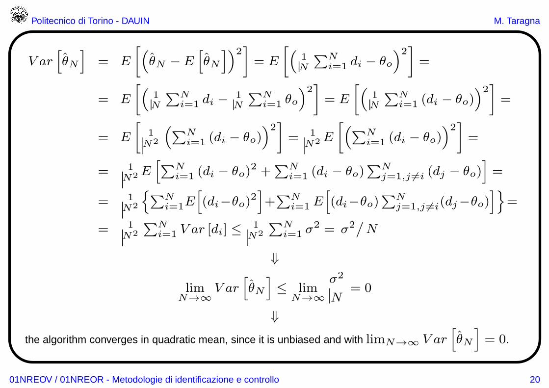
Politecnico di Torino - DAUIN M. Taragna
V ar[
θN
]
= E
[
(
θN − E[
θN
])2]
= E
[
(
1N
∑Ni=1 di − θo
)2]
=
= E
[
(
1N
∑Ni=1 di −
1N
∑Ni=1 θo
)2]
= E
[
(
1N
∑Ni=1 (di − θo)
)2]
=
= E
[
1N2
(
∑Ni=1 (di − θo)
)2]
= 1N2
E
[
(
∑Ni=1 (di − θo)
)2]
=
= 1N2
E[
∑Ni=1 (di − θo)
2 +∑N
i=1 (di − θo)∑N
j=1,j 6=i (dj − θo)]
=
= 1N2
{
∑Ni=1E
[
(di−θo)2]
+∑N
i=1 E[
(di−θo)∑N
j=1,j 6=i(dj−θo)]}
=
= 1N2
∑Ni=1 V ar [di] ≤
1N2
∑Ni=1 σ
2 = σ2/
N
⇓
limN→∞
V ar[
θN
]
≤ limN→∞
σ2
N= 0
⇓
the algorithm converges in quadratic mean, since it is unbiased and with limN→∞ V ar[
θN
]
= 0.
01NREOV / 01NREOR - Metodologie di identificazione e controllo 20

Politecnico di Torino - DAUIN M. Taragna
Estimator #2:
θN = dj
• it is an unbiased estimator:
E[
θN
]
= E [dj ] = θo
• it does not converge in quadratic mean:
V ar[
θN
]
= E
[
(
θN − E[
θN
])2]
= E[
(dj − θo)2]
= V ar [dj ] ≤ σ2
and then it does not vary with the number N of data
⇓
the estimation uncertainty is constant and, in particular, it does not decrease
when the number of data grows.
01NREOV / 01NREOR - Metodologie di identificazione e controllo 21

Politecnico di Torino - DAUIN M. Taragna
Estimator #3 (weighted sample mean):
θN =N∑
i=1
αidi
• it is an unbiased estimator if and only if∑N
i=1 αi = 1, because
E[
θN
]
= E[
∑Ni=1 αidi
]
=∑N
i=1 αiE [di] = θo∑N
i=1αi = θo ⇔∑N
i=1αi = 1
Note: the algorithm #1 corresponds to the case αi =1N
, ∀i;
the algorithm #2 corresponds to the case αj = 1 and αi = 0, ∀i 6= j
• it can be proven that the minimum variance unbiased estimator has weights
αi =α
V ar [di], α =
[N∑
i=1
1
V ar [di]
]−1
intuitively, more uncertain data are considered as less trusted, with lower weights
01NREOV / 01NREOR - Metodologie di identificazione e controllo 22

Politecnico di Torino - DAUIN M. Taragna
• the variance of the minimum variance unbiased estimator is
V ar[
θN
]
= E
[
(
θN − E[
θN
])2]
= E
[
(
∑Ni=1 αidi − θo
)2]
=
= E
[
(
∑Ni=1 αidi −
∑Ni=1 αiθo
)2]
= E
[
(
∑Ni=1 αi (di − θo)
)2]
=
= E[
∑Ni=1 α
2i (di−θo)
2 +∑N
i=1 αi(di−θo)∑N
j=1,j 6=i αj(dj−θo)]
=
=∑N
i=1α2iE[
(di−θo)2]
+∑N
i=1αiE[
(di−θo)∑N
j=1,j 6=iαj(dj−θo)]
=
=∑N
i=1α2i V ar [di]=
∑Ni=1
α2
V ar[di]2V ar[di]= α2
∑Ni=1
1
V ar[di]=
= α =
[
∑Ni=1
1
V ar [di]
]−1
≤
[
∑Ni=1
1
σ2
]−1
=σ2
N
• the minimum variance unbiased algorithm converges in quadratic mean, since
limN→∞
V ar[
θN
]
≤ limN→∞
σ2
N= 0
01NREOV / 01NREOR - Metodologie di identificazione e controllo 23

Politecnico di Torino - DAUIN M. Taragna
Cramer-Rao inequalityThe estimation precision has its own intrinsic limits, due to the random source of data:
in fact, the variance of any estimator cannot be less than a certain value, since data are
always affected by noises and the corresponding uncertainty reflects into a structural
estimate uncertainty, which cannot be suppressed simply by changing the estimator:
• in the scalar case θ ∈ R, the following Cramer-Rao inequality holds
for any unbiased estimator θ:
V ar[
θ]
≥ m−1
where m is the Fisher information quantity defined as
m = E
[
{
∂∂θ
ln f(d(θ), θ)}2]
θ=θo
= −E[
∂2
∂θ2ln f(d(θ), θ)
]
θ=θo≥ 0
d(θ)∈ RN are the data generated by the random source for a generic value θ of the unknown
variable, not necessarily the “true” value θo; f(q,θ), q∈RN, is the probability density function of q;
01NREOV / 01NREOR - Metodologie di identificazione e controllo 24

Politecnico di Torino - DAUIN M. Taragna
• in the vector case θ ∈ Rn, for any unbiased estimator θ,
the Cramer-Rao inequality becomes
V ar[
θ]
≥M−1
where M is the nonsingular Fisher information matrix
M = [mij ] ∈ Rn×n
mij = −E[
∂2
∂θi∂θjln f(d(θ), θ)
]
θ=θo
, ∀i, j = 1, 2, . . . , n
From this inequality it follows that
V ar[
θi
]
≥[M−1
]
ii, ∀i = 1, 2, . . . , n
An unbiased estimator is efficient if it provides the minimum variance, i.e., if its varianceachieves the minimal theoretic value assessed by the Cramer-Rao inequality:
V ar[
θ]
= m−1 or V ar[
θ]
=M−1
01NREOV / 01NREOR - Metodologie di identificazione e controllo 25

Politecnico di Torino - DAUIN M. Taragna
Least Squares estimation methodLinear regression problem : given the measurements of n+ 1 real variables y(t),
u1(t), . . . , un(t) over a time interval (e.g., for t = 1, 2, . . . , N ), find if possible the
values of n real parameters θ1, θ2, . . . , θn such that the following relationship holds
y(t) = θ1u1(t) + . . .+ θnun(t)
In matrix terms, by defining the real vectors
θ =
θ1...θn
∈ R
n, ϕ(t) =
u1(t)...
un(t)
∈ R
n ⇒ y(t) = ϕ(t)Tθ
In the actual problems, there exists always a nonzero error ε(t)=y(t)− ϕ(t)Tθ
⇓
by defining J(θ)=N∑
t=1ε(t)
2, the problem is solved by finding θ∗= argmin
θ∈Rn
J(θ).
01NREOV / 01NREOR - Metodologie di identificazione e controllo 26

Politecnico di Torino - DAUIN M. Taragna
In order to find the minimum of the figure of merit J , we have to require that
dJ(θ)
dθ=
[
dJ(θ)
dθ1. . .
dJ(θ)
dθn
]
= 0 ⇔
dJ(θ)
dθi=
d
dθi
[
N∑
t=1ε(t)2
]
=N∑
t=1
d
dθi
[
ε(t)2]
=N∑
t=1
d
dθi
[
(
y(t)− ϕ(t)T θ)2]
=
= −2N∑
t=1
(
y(t)− ϕ(t)T θ)
ui(t) = 0, i = 1, 2, . . . , n ⇔
dJ(θ)
dθ= −2
N∑
t=1
(
y(t)− ϕ(t)T θ)
ϕ(t)T = 0 ⇔
N∑
t=1
(
y(t)ϕ(t)T − ϕ(t)T θϕ(t)T)
=N∑
t=1y(t)ϕ(t)T −
N∑
t=1ϕ(t)T θϕ(t)T = 0 ⇔
N∑
t=1ϕ(t)T θϕ(t)T =
N∑
t=1y(t)ϕ(t)T ⇔
N∑
t=1
[
ϕ(t)ϕ(t)T]
θ =N∑
t=1ϕ(t) y(t)
01NREOV / 01NREOR - Metodologie di identificazione e controllo 27

Politecnico di Torino - DAUIN M. Taragna
The relationshipN∑
t=1
[
ϕ(t)ϕ(t)T]
θ =N∑
t=1ϕ(t) y(t)
is a system of n scalar equations involving n scalar unknowns θ1, θ2, . . . , θn that is
called normal equation system :
• if the matrixN∑
t=1ϕ(t)ϕ(t)
Tis nonsingular (⇔ det
N∑
t=1ϕ(t)ϕ(t)
T 6= 0, known
as identifiability condition), then the normal equation system has a single unique
solution given by the Least Squares (LS) estimate :
θ =
[N∑
t=1ϕ(t)ϕ(t)
T
]−1 [N∑
t=1ϕ(t) y(t)
]
• ifN∑
t=1ϕ(t)ϕ(t)
Tis singular, it can be proved that the normal equations have an
infinite number of solutions, due to their particular structure.
01NREOV / 01NREOR - Metodologie di identificazione e controllo 28

Politecnico di Torino - DAUIN M. Taragna
The stationarity conditiondJ(θ)dθ
=0 does not guarantee that θ is a minimum of J(θ)⇒ we have to consider the Hessian matrix
d2J(θ)
dθ2=
d
dθ
[
dJ(θ)
dθ
]T
=d
dθ
[
−2∑N
t=1
(
y(t)− ϕ(t)T θ)
ϕ(t)T]T
=
=d
dθ
[
−2∑N
t=1
(
y(t)ϕ(t)T − θTϕ(t)ϕ(t)T)T]
=
=d
dθ
[
−2∑N
t=1 y(t)ϕ(t) + 2∑N
t=1 ϕ(t)ϕ(t)T θ]
=
= 2N∑
t=1
d
dθϕ(t)ϕ(t)T θ = 2
N∑
t=1ϕ(t)ϕ(t)T
that turns out to be positive semidefinite, since ∀x ∈ Rn
xT d2J(θ)
dθ2x = xT 2
N∑
t=1ϕ(t)ϕ(t)T x = 2
N∑
t=1xTϕ(t)ϕ(t)T x = 2
N∑
t=1
(
xTϕ(t))2
≥ 0
⇓
θ is certainly a (local or global) minimum of J(θ).
01NREOV / 01NREOR - Metodologie di identificazione e controllo 29

Politecnico di Torino - DAUIN M. Taragna
The Taylor series expansion of J(θ) in the neighborhood of θ allows to understand if
θ is a local or global minimum:
J(θ)=J(θ)+dJ(θ)dθ
∣
∣
∣
θ(θ− θ)+ 1
2(θ− θ)T
d2J(θ)
dθ2
∣
∣
∣
θ(θ− θ)+ . . .=J(θ)+1
2(θ− θ)T
d2J(θ)
dθ2
∣
∣
∣
θ(θ− θ)
since the termdJ(θ)dθ
∣
∣
∣
θ=θis zero (θ is a minimum) as well as all the J(θ) derivatives of order greater
than two (J(θ) is a quadratic function of θ)⇓
J(θ)− J(θ) = 12(θ − θ)T
d2J(θ)
dθ2
∣
∣
∣
θ(θ − θ),
d2J(θ)
dθ2
∣
∣
∣
θ= 2
∑Nt=1 ϕ(t)ϕ(t)
T ,
is a positive semidefinite quadratic form, sinced2J(ϑ)dϑ2
∣∣∣θ
is positive semidefinite:
• if∑N
t=1 ϕ(t)ϕ(t)T
is nonsingular ⇒ d2J(θ)dθ2
∣∣∣θ
is positive definite ⇒
the quadratic form is positive definite and it is a paraboloid with a unique minimum
⇒ θ is the global minimum of J(θ);
• if∑N
t=1 ϕ(t)ϕ(t)T
is singular ⇒ the quadratic form is positive semidefinite
and it has an infinite number of local minima, aligned over a line tangent to J(θ).
01NREOV / 01NREOR - Metodologie di identificazione e controllo 30

Politecnico di Torino - DAUIN M. Taragna
The obtained results may be rewritten in a compact matrix form by defining:
Φ=
ϕ(1)T...
ϕ(N)T
=
u1(1) . . . un(1)...
.
.
.u1(N) . . . un(N)
∈ R
N×n, y =
y(1)...
y(N)
∈ R
N
⇓
y(t) = ϕ(t)Tθ, t = 1, 2, . . . , N ⇔ y = Φθ
⇓∑N
t=1 ϕ(t)ϕ(t)T= ΦTΦ,
∑N
t=1 ϕ(t) y(t) = ΦT y
⇓the normal equation system becomes:
ΦTΦθ = ΦT yand, if ΦTΦ is nonsingular (identifiability condition), it has a unique solution given by
the least squares estimate:
θLS =[ΦTΦ
]−1ΦTy
01NREOV / 01NREOR - Metodologie di identificazione e controllo 31

Politecnico di Torino - DAUIN M. Taragna
Probabilistic characteristics of least squares estimator
Assumptions:
• the identifiability condition holds: ∃[ΦTΦ
]−1;
• the random source of data has the following structure
y(t) = ϕ(t)T θo + v(t) , t = 1, 2, . . . , N
where v(t) is a zero-mean random disturbance ⇒
the relationship between y and u1, u2, . . . , un is assumed to be linear ⇒
there exists a “true” value θo of the unknown variable;
in compact matrix form, it results that:
y = Φθo + v
where v =
v(1)...
v(N)
∈ R
N is a vector random variable with E [v] = 0.
01NREOV / 01NREOR - Metodologie di identificazione e controllo 32

Politecnico di Torino - DAUIN M. Taragna
Under these assumptions, the least squares estimator becomes:
θ = [ΦTΦ]−1ΦT y = [ΦTΦ]−1ΦT (Φθo + v) =
= [ΦTΦ]−1ΦTΦθo + [ΦTΦ]−1ΦT v = θo + [ΦTΦ]−1ΦT v
and it has the following probabilistic characteristics:
• it is unbiased , since its mean value E[θ ] = θo
E[θ ] = E[
[
ΦTΦ]−1
ΦT y]
=[
ΦTΦ]−1
ΦTE[y] =[
ΦTΦ]−1
ΦTE[Φθo + v] =
=[
ΦTΦ]−1
ΦT (Φθo +E[v]) =[
ΦTΦ]−1
ΦTΦθo = θo
• if v is a vector of zero-mean random variables that are uncorrelated and with thesame varianceσ2
v (V ar[v]=E[
vvT]
=σ2vIN ), as in the case of disturbance v(·)
given by a white noise WN(0, σ2v) ⇒ V ar[θ ] = σ2
v[ΦTΦ]−1
V ar[θ ] = E[
(θ −E[θ])(θ −E[θ])T]
= E[
(θ − θo)(θ − θo)T]
=
= E[
(
[ΦTΦ]−1ΦTv)(
[ΦTΦ]−1ΦTv)T]
=E[
[ΦTΦ]−1ΦTvvTΦ[ΦTΦ]−1]
=
= [ΦTΦ]−1ΦTE[
vvT]
Φ[ΦTΦ]−1 = [ΦTΦ]−1ΦT σ2vINΦ[ΦTΦ]−1 =
= σ2v[Φ
TΦ]−1ΦTΦ[ΦTΦ]−1 = σ2v[Φ
TΦ]−1
01NREOV / 01NREOR - Metodologie di identificazione e controllo 33

Politecnico di Torino - DAUIN M. Taragna
• The variance σ2v of the disturbance v is usually unknown ⇒
under the same previous assumptions, a “reasonable” unbiased estimate σ2v
(such that E[σ2v] = σ2
v) can be directly derived from data as
σ2v =
J(θ)
N − nwhere N = measurement number, n = number of unknown parameters of θ,
J(θ) =∑N
t=1 ε(t)2∣
∣
∣
θ=θ=∑N
t=1
[
y(t)− ϕ(t)T θ]2
= [y − Φθ]T [y − Φθ] =
=(
(IN − Φ[ΦTΦ]−1ΦT )y)T
(IN − Φ[ΦTΦ]−1ΦT )y =
= yT (IN − Φ[ΦTΦ]−1ΦT )(IN − Φ[ΦTΦ]−1ΦT )y =
= yT (IN − 2Φ[ΦTΦ]−1ΦT + Φ[ΦTΦ]−1ΦTΦ[ΦTΦ]−1ΦT )y =
= yT (IN − Φ[ΦTΦ]−1ΦT )y
⇓
V ar[θ ] = σ2v[Φ
TΦ]−1 ∼= σ2v[Φ
TΦ]−1
01NREOV / 01NREOR - Metodologie di identificazione e controllo 34

Politecnico di Torino - DAUIN M. Taragna
Weighted Least Squares estimation method
With the least squares estimation method, all the errors have the same relevance,
since the figure of merit to be minimized is
JLS(θ)=∑N
t=1ε(t)2
, where ε(t)=y(t)− ϕ(t)Tθ, t = 1, 2, . . . , N.
However, if some measurements are more accurate than some others, different
relevance can be assigned to the errors, by defining the figure of merit
JWLS(θ)=N∑
t=1q(t) ε(t)
2= εTQε
where q(t) are the weighting coefficients (or weights ) for t = 1, 2, . . . , N ,
Q = diag (q(t)) =
q(1) 0 . . . 0
0 q(2) . . . 0
. . . . . . . . . . . .
0 0 . . . q(N)
∈ RN×N , ε =
ε(1)...
ε(N)
∈ R
N .
01NREOV / 01NREOR - Metodologie di identificazione e controllo 35

Politecnico di Torino - DAUIN M. Taragna
The Weighted Least Squares (WLS) estimate minimizes the figure of meritJWLS(θ):
θWLS=[ΦTQΦ
]−1ΦTQy
If the disturbance v is a vector of zero-mean uncorrelated random variables withvariance Σv , the estimator θWLS has the following probabilistic characteristics:
• it is unbiased , since its mean value E[θWLS ] = θo
E[θWLS ] =E[
[
ΦTQΦ]−1
ΦTQy]
=[
ΦTQΦ]−1
ΦTQE[y]=[
ΦTQΦ]−1
ΦTQE[Φθo+v]=
=[
ΦTQΦ]−1
ΦTQ (Φθo +E[v]) =[
ΦTQΦ]−1
ΦTQΦθo = θo
• its variance is
V ar[θWLS ] =E[(θWLS−E[θWLS ])(θWLS−E[θWLS ])T ] =
=E[(θWLS−θo)(θWLS−θo)T ] = E[
(
[ΦTQΦ]−1ΦTQv)(
[ΦTQΦ]−1ΦTQv)T]
=
=E[
[ΦTQΦ]−1ΦTQvvTQTΦ[ΦTQΦ]−1]
=
=[ΦTQΦ]−1ΦTQE[
vvT]
QΦ[ΦTQΦ]−1 = [ΦTQΦ]−1ΦTQΣvQΦ[ΦTQΦ]−1
and then it depends on the disturbance variance Σv ;
01NREOV / 01NREOR - Metodologie di identificazione e controllo 36

Politecnico di Torino - DAUIN M. Taragna
• it can be proved that the best choice for Q that minimizes V ar[θWLS ] is
Q∗ = argminQ=diag(q(t))∈Rn×n
V ar[θWLS ] = Σ−1v
and in this case we obtain the so-called Gauss-Markov estimate :
θGM=[ΦTΣ−1
v Φ]−1
ΦTΣ−1v y
whose variance is
V ar[θGM ]= [ΦTQΦ]−1ΦTQΣvQΦ[ΦTQΦ]−1 =
= [ΦTΣ−1v Φ]−1ΦTΣ−1
v ΣvQΦ[ΦTΣ−1v Φ]−1
= [ΦTΣ−1v Φ]−1 ;
If in particular it results that Σv = σ2vIN ⇒
θGM =[
ΦT 1σ2v
INΦ]−1
ΦT 1σ2v
INy =[ΦTΦ
]−1ΦT y = θLS
01NREOV / 01NREOR - Metodologie di identificazione e controllo 37

Politecnico di Torino - DAUIN M. Taragna
Maximum Likelihood estimatorsThe actual data are generated by a random source, which depends on the outcome s
of a random experiment and on the “true” value θo of the unknown to be estimated.
However, if a generic value θ of the unknown parameter is considered, the data can
be seen as function of both the value θ and the outcome s ⇒
the data can be denoted by d(θ)(s), with p.d.f. f(q, θ) that is function of θ too.
Let δ be the particular data observation that corresponds to a particular outcome s of
the random experiment:δ = d(θ)(s)
The so-called likelihood function is given by the p.d.f. of the data evaluated in δ:
L(θ) = f(q, θ)|q=δ
The Maximum Likelihood (ML) estimate is defined as:
θML= argmaxθ∈Rn
L(θ)
01NREOV / 01NREOR - Metodologie di identificazione e controllo 38
Politecnico di Torino - DAUIN M. Taragna
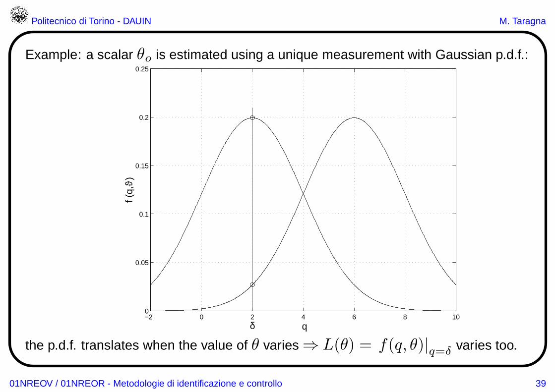
Example: a scalar θo is estimated using a unique measurement with Gaussian p.d.f.:
−2 0 2 4 6 8 100
0.05
0.1
0.15
0.2
0.25
q
f (q,
ϑ)
δ
the p.d.f. translates when the value of θ varies ⇒ L(θ) = f(q, θ)|q=δ varies too.
01NREOV / 01NREOR - Metodologie di identificazione e controllo 39

Politecnico di Torino - DAUIN M. Taragna
Maximum Likelihood estimator properties
The estimate θML is:
• asymptotically unbiased: E(
θML
)
−−−−−−→N → ∞
θo
• asymptotically efficient: ΣθML
≤ Σθ
∀θ if N → ∞
• consistent: limN→∞
ΣθML
= 0
• asymptotically Gaussian (for N → ∞)
01NREOV / 01NREOR - Metodologie di identificazione e controllo 40

Politecnico di Torino - DAUIN M. Taragna
Example : let us assume that the random source of data has the following structure:
y(t) = ψ(t, θo) + v(t) , t = 1, 2, . . . , N ⇔ y = Ψ(θo) + v
where ψ(t, θo) is a generic nonlinear function of θo and the disturbance v is a
vector of zero-mean Gaussian random variables with variance Σv and p.d.f.
f(q) = N (0,Σv) =1
√
(2π)N detΣv
exp(
− 12qTΣ−1
v q)
Since v = y −Ψ(θo)⇒ the p.d.f. of data generated by a random source where a
generic value θ is considered instead of θo is then given by
f(q, θ) =1
√
(2π)N detΣv
exp(
− 12[q −Ψ(θ)]T Σ−1
v [q −Ψ(θ)])
⇓
L(θ) = f(q, θ)|q=δ
=1
√
(2π)N detΣv
exp(
− 12[δ −Ψ(θ)]T Σ−1
v [δ −Ψ(θ)])
01NREOV / 01NREOR - Metodologie di identificazione e controllo 41

Politecnico di Torino - DAUIN M. Taragna
L(θ) = f(q, θ)|q=δ
=1
√
(2π)N detΣv
exp(
− 12[δ −Ψ(θ)]T Σ−1
v [δ −Ψ(θ)])
⇓
f(q, θ)|q=δ is an exponential function of θ
⇓
θML= argmaxθ∈Rn
L(θ) =argminθ∈Rn
{
[δ −Ψ(θ)]TΣ−1
v [δ −Ψ(θ)]
︸ ︷︷ ︸
R(θ)
}
Problem: the global minimum of R(θ) has to be found with respect to θ, but R(θ)
may have many local minima if Ψ(θ) is a generic nonlinear function of the unknown
variable; the standard nonlinear optimization algorithms do not guarantee to find
always the global minimum.
01NREOV / 01NREOR - Metodologie di identificazione e controllo 42

Politecnico di Torino - DAUIN M. Taragna
Particular case: Ψ(θ) = linear function of the unknown parameters = Φθ
⇓
R (θ) is a quadratic function of θ : R (θ) = [δ − Φθ]TΣ−1
v [δ − Φθ]
⇓
there exists a unique minimum of R (θ)
⇓
θML =(ΦTΣ−1
v Φ)−1
ΦTΣ−1v δ = Gauss-Markov estimate = θGM =
= Weighted Least Squares estimate using the disturbance variance
If Σv = σ2vIN , i.e., independent identically distributed (i.i.d.) disturbance:
θML = θGM =(ΦTΦ
)−1ΦT δ = Least Squares estimate
01NREOV / 01NREOR - Metodologie di identificazione e controllo 43

Politecnico di Torino - DAUIN M. Taragna
Gauss-Markov estimate properties
The estimate θGM is:
• unbiased: E(
θGM
)
= θo
• efficient: ΣθGM
≤ Σθ
∀θ
• consistent: limN→∞
ΣθGM
= 0
• Gaussian
01NREOV / 01NREOR - Metodologie di identificazione e controllo 44

Politecnico di Torino - DAUIN M. Taragna
Bayesian estimation method
The Bayesian method allows one to take into account experimental data and a priori
information on the unknown of the estimation problem that, if well exploited, can
improve the estimate and make up for possible random errors corrupting the data:
• the unknown θ is considered as a random variable, whose a priori p.d.f. (i.e.,
in absence of data) has some given behaviour, mean value and variance
⇓
the mean value is a possible estimate of θ and the variance represents a priori
uncertainty;
• as new experimental data arrive, the p.d.f. of θ is updated on the basis of the new
information: the mean value changes with respect to the a priori one, while the
variance is expected to decrease thanks to the information provided by data.
01NREOV / 01NREOR - Metodologie di identificazione e controllo 45

Politecnico di Torino - DAUIN M. Taragna
A joint random experiment E = E1 × E2 is assumed to exist, whose joint outcome sis the couple of single outcomes s1 and s2: s = (s1, s2):
• the unknown θ is generated by a first random source S1 on the basis ofthe outcome s1 of the first random experiment E1 ⇒ θ = θ(s1);
• the data d are generated by the second random source S2, influenced by
– the outcome s2 of the second random experiment E2– the value θ(s1) of the unknown to be estimated
d = d(s2, θ(s1))
A generic estimator is a function of data θ = h(d) and its performances improveas much as the estimate θ is closer to the unknown to be estimated
⇓by considering as figure of merit
J(h(·)) = E[‖θ − h(d)‖2]the Bayesian optimal estimator is the particular function h∗(·) such that
E[‖θ − h∗(d)‖2] ≤ E[‖θ − h(d)‖2], ∀h(·)
01NREOV / 01NREOR - Metodologie di identificazione e controllo 46

Politecnico di Torino - DAUIN M. Taragna
It can be proved that such an optimal estimator exists and it is given by:
h∗(x) = E [θ| d = x]
where x is the current value that the data d may take.
The Bayesian estimator (or conditional mean estimator ) is the function
θ = E [θ|d]
and the Bayesian estimate (or conditional mean estimate ) is the numeric value
θ = E [θ| d = δ]
where δ is the value of the data d that corresponds to a particular outcome of the
joint random experiment E .
01NREOV / 01NREOR - Metodologie di identificazione e controllo 47

Politecnico di Torino - DAUIN M. Taragna
Bayesian estimator in the Gaussian case
Assumption : the data d and the unknown θ are scalar random variables with zero
mean value and both are individually and jointly Gaussian:[
d
θ
]
∼ N
([
0
0
]
,Σ=V ar
[
d
θ
]
=
[
σdd σdθ
σθd σθθ
])
⇒ their joint p.d.f. is given by:
f(d, θ) = C exp
{
−1
2[ d θ ] Σ
−1 [ d θ ]T
}
, C : suitable constant
Since
detΣ = det
[
σdd σdθ
σθd σθθ
]
= σddσθθ−σ2dθ = σdd
(
σθθ−σ2θd
σdd
)
= σdd σ2,
where σ2 = σθθ− σ2θd
/
σdd ≤ σθθ
⇓
Σ−1 =1
detΣ
[
σθθ −σdθ
−σθd σdd
]
=1
σ2
[
σθθ/σdd −σdθ/σdd
−σθd/σdd 1
]
01NREOV / 01NREOR - Metodologie di identificazione e controllo 48

Politecnico di Torino - DAUIN M. Taragna
⇓
f(d, θ) =C exp
{
−1
2σ2[ d θ ]
[
σθθ/σdd −σdθ/σdd
−σθd/σdd 1
][
d
θ
]}
=
=C exp
{
−1
2σ2[ d θ ]
[
σθθ/σdd d− σdθ/σdd θ
−σθd/σdd d+ θ
]}
=
=C exp
{
−1
2σ2
(
σθθ
σdd
d2 − 2σθd
σdd
dθ + θ2)}
The p.d.f. of the data d is given by:
f(d) = C′ exp
{
−d2
2σdd
}
, C′ : suitable constant
⇓
the p.d.f. of the unknown θ conditioned by data d is equal to:
f(θ|d) =f(d, θ)
f(d)=
C
C′exp
{
−1
2σ2
(
σθθ
σdd
d2 − 2σθd
σdd
dθ + θ2)
+d2
2σdd
}
=
=C′′exp
{
−1
2σ2
[
σ2dθ
σ2dd
d2− 2σθd
σdd
dθ + θ2
]}
=C′′exp
{
−1
2σ2
[
θ −σθd
σdd
d
]2}
01NREOV / 01NREOR - Metodologie di identificazione e controllo 49

Politecnico di Torino - DAUIN M. Taragna
⇓
f(θ|d) = C′′exp
{
− 12σ2
[
θ − σθd
σdd
d]2}
∼ N(
σθd
σdd
d, σ2)
The Bayesian estimator is the function
θ = E [θ| d] = σθd
σddd
while the Bayesian estimate corresponding to the particular observation δ of data dis the numerical value
θ = E [θ| d = δ] = σθd
σddδ
Since E [d] = E [θ] = 0⇒
E[θ] = E[
σθd
σddd]
= σθd
σddE [d] = 0
V ar[θ ] = E[(θ −E[θ ])2] = E[θ2] = E
[
σ2
θd
σ2
dd
d2]
=σ2
θd
σ2
dd
E[
d2]
=σ2
θd
σdd
V ar[θ − θ ] =E[(θ − θ)2] = E[(θ − σθd
σdd
d)2] = E[θ2− 2σθd
σdd
θd+σ2
θd
σ2
dd
d2] =
=E[
θ2]
− 2σθd
σdd
E [θd ] +σ2
θd
σ2
dd
E[
d2]
= σθθ − 2σθd
σdd
σθd +σ2
θd
σ2
dd
σdd =
=σθθ − 2σ2
θd
σdd
+σ2
θd
σdd
= σθθ −σ2
θd
σdd
= σ2
01NREOV / 01NREOR - Metodologie di identificazione e controllo 50

Politecnico di Torino - DAUIN M. Taragna
Optimal linear estimatorAssumption : both the data d and the unknown θ are scalar random variables with
zero mean value and variance matrix V ar
[
d
θ
]
=
[
σdd σdθ
σθd σθθ
]
.
Goal: estimate θ by means of a linear estimator whose structure is
θ = αd+ β
with α, β real parameters, estimated by minimizing the mean squared error (MSE):
J = E[(θ − θ)2] = E[(θ − αd− β)2] = J(α, β)m
∂J∂α
= ∂∂α
E[
(θ − αd− β)2]
= E[
∂∂α
(θ − αd− β)2]
= E [−2(θ − αd− β)d] =
= −2E [θd] + 2αE[
d2]
+ 2βE [d] = −2σdθ + 2ασdd = 0
∂J∂β
= ∂∂β
E[
(θ − αd− β)2]
= E[
∂∂β
(θ − αd− β)2]
= E [−2(θ − αd− β)] =
= −2E [θ] + 2αE [d] + 2β = 2β = 0
m{
α = σθd/σdd
β = 0⇒ θ = σdθ
σddd ≡ E [θ| d]
01NREOV / 01NREOR - Metodologie di identificazione e controllo 51
Politecnico di Torino - DAUIN M. Taragna
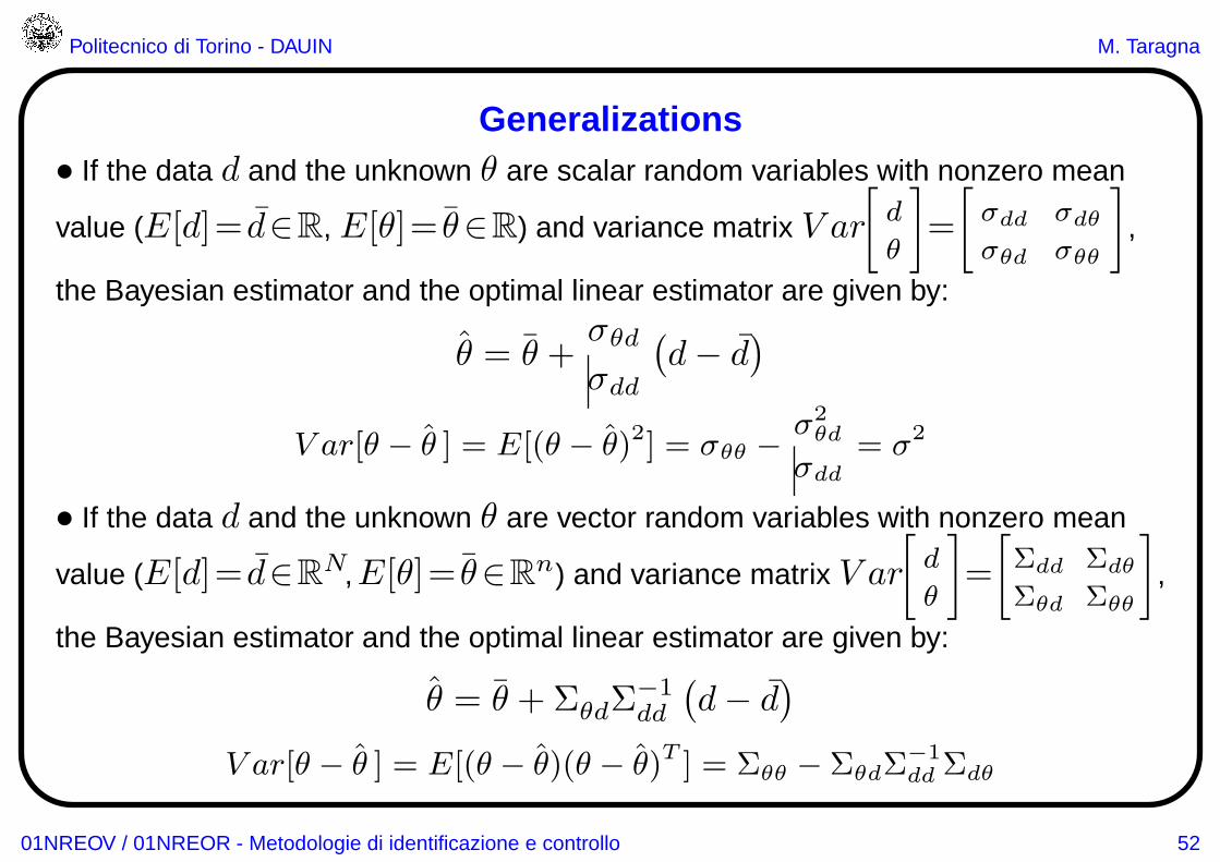
Generalizations• If the data d and the unknown θ are scalar random variables with nonzero mean
value (E[d]= d∈R, E[θ]= θ∈R) and variance matrix V ar
[
d
θ
]
=
[
σdd σdθ
σθd σθθ
]
,
the Bayesian estimator and the optimal linear estimator are given by:
θ = θ +σθd
σdd
(d− d
)
V ar[θ − θ ] = E[(θ − θ)2] = σθθ −σ2θd
σdd
= σ2
• If the data d and the unknown θ are vector random variables with nonzero mean
value (E[d]= d∈RN,E[θ]= θ∈R
n) and variance matrix V ar
[
d
θ
]
=
[
Σdd Σdθ
Σθd Σθθ
]
,
the Bayesian estimator and the optimal linear estimator are given by:
θ = θ + ΣθdΣ−1dd
(d− d
)
V ar[θ − θ ] = E[(θ − θ)(θ − θ)T ] = Σθθ − ΣθdΣ−1dd Σdθ
01NREOV / 01NREOR - Metodologie di identificazione e controllo 52

Politecnico di Torino - DAUIN M. Taragna
Remarks
Remark #1 :
• Using the a priori information only (i.e., in absence of data), a reasonable initialestimate of the unknown is given by the a priori estimate
θ = θprior
= E [θ] = θ
and the corresponding a priori uncertainty is V ar[θ] = Σθθ
• Using also the a posteriori information (i.e., the data), the estimate changes andthe a posteriori estimate in the scalar case is given by
θ = θposterior
= θ +σθd
σdd
(d− d
)= θ
prior+σθd
σdd
(d− d
)
– if σθd = 0, i.e., if d and θ are uncorrelated ⇒ θposterior
= θprior
– if σθd > 0 ⇒ θposterior
− θprior
and d−d have the same sign
– if σθd < 0 ⇒ θposterior
− θprior
and d−d have opposite sign
01NREOV / 01NREOR - Metodologie di identificazione e controllo 53

Politecnico di Torino - DAUIN M. Taragna
Remark #2 : the a posteriori estimate in the scalar case is given by
θ = θposterior
= θ + σθd
σdd
(d− d
)= θ
prior+ σθd
σdd
(d− d
)
– if σdd is high, i.e., if the observation d is affected by great uncertainty ⇒
θ mainly depends on θprior
instead on the term σθd
σdd
(d− d
)
– if σdd is low, i.e., if the observation d is affected by small uncertainty ⇒
θ strongly depends on the term σθd
σdd
(d− d
)that corrects θ
prior
Remark #3 : the estimation error variance represents the a posteriori uncertainty :
V ar[θ− θ ] = E[(θ− θ)2] = σθθ−σ2
θd
σdd= σθθ
(
1− σ2
θd
σθθσdd
)
= σθθ
(1− ρ2
)
where ρ= σθd√σθθσdd
is the correlation coefficient between θ and d, such that |ρ|≤1
– if ρ = 0, i.e., if d and θ are uncorrelated ⇒the a posteriori uncertainty turns out to be equal to the a priori one
– if ρ 6= 0 ⇒ the a posteriori uncertainty is smaller than the a priori one
01NREOV / 01NREOR - Metodologie di identificazione e controllo 54

Politecnico di Torino - DAUIN M. Taragna
Geometrical interpretation
• Let G be the set of the real scalar random variables v with zero mean value, whosevalue v(s) depends on the outcome s of the underlying random experiment E .
• Let G be the vector space defined on G such that, ∀v1, v2∈G and ∀µ∈R, thenv1+v2∈G and µv1∈G; let G be equipped with the inner (or scalar) product:
〈v1, v2〉 = E [v1v2]
that satisfies the following properties, ∀v, v1, v2 ∈ G and ∀µ ∈ R:
(i) 〈v, v〉 = V ar[v] ≥ 0 (nonnegativity)(ii) 〈v, v〉 = 0 if and only if v ∼ (0, 0)
}
(positive-definiteness)
(iii) 〈v, v1 + v2〉 = 〈v, v1〉+ 〈v, v2〉 (additivity)(iv) 〈v1, µv2〉 = µ 〈v1, v2〉 (homogeneity)(v) 〈v1, v2〉 = 〈v2, v1〉 (symmetry)
Such an inner product allows to naturally define a norm on G as:
‖v‖ =√
〈v, v〉 =√
V ar[v]
01NREOV / 01NREOR - Metodologie di identificazione e controllo 55

Politecnico di Torino - DAUIN M. Taragna
• Any random variable v is a vector in the space G with “length” ‖v‖ =√
V ar[v]
• Given two random variables v1 and v2, the angle α between the corresponding
vectors in G is involved in the inner product, since:
〈v1, v2〉 = ‖v1‖ ‖v2‖ cosα
⇓
cosα =〈v1, v2〉
‖v1‖ ‖v2‖=
E [v1v2]√
V ar[v1]√
V ar[v2]= ρ
– ρ = 0 ⇔ v1 and v2 are uncorrelated ⇔the corresponding vectors in G are orthogonal, i.e., v1 ⊥ v2
– ρ = ±1 ⇔ the vectors corresponding to v1 and v2 are parallel, i.e., v1//v2 :
if v2 = αv1 + β, with α, β∈R and α > 0, then ρ = +1if v2 = αv1 + β, with α, β∈R and α < 0, then ρ = −1
01NREOV / 01NREOR - Metodologie di identificazione e controllo 56

Politecnico di Torino - DAUIN M. Taragna
• In the scalar Gaussian case, the Bayesian estimate of v2 given v1 is:
v2 = E [v2| v1] =σ21
σ11
v1, where σ21 = E [v1v2] , σ11 = V ar[v1]
⇓
v2=E[v1v2]
V ar[v1]v1=
〈v1,v2〉
‖v1‖2 v1=
1
‖v1‖
〈v1,v2〉
‖v1‖
1
‖v2‖︸ ︷︷ ︸
cosα
‖v2‖v1=‖v2‖ cosαv1‖v1‖
the Bayesian estimate v2 has the same direction of v1 with “length” ‖v2‖ cosα,i.e., v2 is the orthogonal projection of v2 over v1
αv1
v2
1 1v v 2 1
E v v
αv1
v2
1 1v v 2 1
E v v
01NREOV / 01NREOR - Metodologie di identificazione e controllo 57

Politecnico di Torino - DAUIN M. Taragna
•The estimation error variance of v2 given v1 (i.e., the a posteriori uncertainty) is:
V ar[v2−E[v2|v1]]=σ22−σ2
21
σ11
, with σ22=V ar[v2],σ21=E[v1v2] ,σ11=V ar[v1]
⇓
V ar[v2−E[v2|v1]]=V ar[v2]−E[v1v2]
2
V ar[v1]=‖v2‖
2−‖E[v2|v1]‖2=‖v2−E[v2|v1]‖
2
i.e., it can be computed by evaluating the “length” of the vector v2 −E [v2| v1]
through the Pythagorean theorem
αv1
v2
1 1v v 2 1
E v v
2 2 1v E v v
−α
v1
v2
1 1v v 2 1
E v v
2 2 1v E v v
−
•The generalization of the geometric interpretation to the vector case is straightforward
01NREOV / 01NREOR - Metodologie di identificazione e controllo 58

Politecnico di Torino - DAUIN M. Taragna
Recursive Bayesian estimation: scalar case
Assumptions : the unknownθ is a scalar random variable with zero mean value; the datavector d is a random variable having 2 components d(1),d(2), with zero mean value:
θ
d(1)
d(2)
∼
0
0
0
,Σ=V ar
θ
d(1)
d(2)
=
σθθ σθ1 σθ2
σ1θ σ11 σ12
σ2θ σ21 σ22
,
σθ1=σ1θ
σθ2=σ2θ
σ12=σ21
• The optimal linear estimate of θ based on d(1) only is given by:
E [θ| d(1)] =σθ1
σ11d(1)
• The optimal linear estimate of θ based on d(1) and d(2) is given by:
E [θ| d(1), d(2)] = ΣθdΣ−1dd d = [σθ1 σθ2 ]
[
σ11 σ12
σ21 σ22
]−1 [
d(1)
d(2)
]
01NREOV / 01NREOR - Metodologie di identificazione e controllo 59

Politecnico di Torino - DAUIN M. Taragna
Since
detΣdd = det
σ11 σ12
σ21 σ22
= σ11σ22−σ221 = σ11
(
σ22−σ221
σ11
)
= σ11 σ2,
where σ2 = σ22−σ221
σ11
⇓
Σ−1dd
=1
detΣdd
σ22 −σ12
−σ21 σ11
=1
σ2
σ22/σ11 −σ12/σ11
−σ21/σ11 1
⇓
E [ θ| d(1), d(2)] = Σθd
Σ−1dd
d = [ σθ1 σθ2 ]1
σ2
σ22/σ11 −σ12/σ11
−σ21/σ11 1
[
d(1)
d(2)
]
=
=1
σ2
[
σθ1σ22
σ11− σθ2
σ21
σ11σθ2 − σθ1
σ12
σ11
]
[
d(1)
d(2)
]
=
=1
σ2
(
σθ1σ22
σ11− σθ2
σ21
σ11
)
d(1) +1
σ2
(
σθ2 − σθ1σ12
σ11
)
d(2)
01NREOV / 01NREOR - Metodologie di identificazione e controllo 60

Politecnico di Torino - DAUIN M. Taragna
By adding and subtracting the term E [θ| d(1)] =σθ1
σ11d(1) and recalling that
σ12 = σ21 and σ2 = σ22−σ221
σ11, it results that:
E [ θ| d(1), d(2)] =
= 1σ2
(
σθ1σ22
σ11
−σθ2σ21
σ11
)
d(1) + 1σ2
(
σθ2−σθ1σ12
σ11
)
d(2) + σθ1
σ11
d(1)− σθ1
σ11
d(1)=
= σθ1
σ11
d(1) + 1σ2
(
σθ1σ22
σ11
−σθ2σ21
σ11
− σθ1
σ11
σ2)
d(1) + 1σ2
(
σθ2−σθ1σ12
σ11
)
d(2)=
= σθ1
σ11
d(1) + 1σ2
(
σθ1σ22
σ11
−σθ2σ21
σ11
− σθ1
σ11
σ22+σθ1
σ11
σ2
21
σ11
)
d(1) + 1σ2
(
σθ2−σθ1σ12
σ11
)
d(2)
= σθ1
σ11
d(1) + 1σ2
(
−σθ2σ21
σ11
+ σθ1σ2
21
σ2
11
)
d(1) + 1σ2
(
σθ2 − σθ1σ12
σ11
)
d(2)=
= σθ1
σ11
d(1)− 1σ2
σ21
σ11
(
σθ2 − σθ1σ21
σ11
)
d(1) + 1σ2
(
σθ2 − σθ1σ12
σ11
)
d(2)=
= σθ1
σ11
d(1) + 1σ2
(
σθ2 − σθ1σ21
σ11
) [
d(2)− σ21
σ11
d(1)]
=
=E [ θ| d(1)] + 1σ2
(
σθ2 − σθ1σ21
σ11
)
[d(2)− E [d(2)| d(1)]]
01NREOV / 01NREOR - Metodologie di identificazione e controllo 61

Politecnico di Torino - DAUIN M. Taragna
Definition : given two scalar random variables d(1) and d(2) with zero mean value,
the innovation of d(2) given d(1) is the scalar random variable defined by:
e = d(2)− E [d(2)| d(1)] = d(2)− σ21
σ11
d(1)
• E[e] = E[
d(2)− σ21
σ11
d(1)]
= E[d(2)]− σ21
σ11
E[d(1)] = 0
• σee = V ar[e] = E[
(e−E [e])2]
= E[
e2]
= E
[
(
d(2)− σ21
σ11
d(1))2]
=
=E
[
d2(2)−2σ21
σ11
d(2)d(1)+σ2
21
σ2
11
d2(1)
]
=E[
d2(2)]
−2σ21
σ11
E[d(2)d(1)]+σ2
21
σ2
11
E[
d2(1)]
=σ22 − 2σ21
σ11
σ21 +σ2
21
σ2
11
σ11 = σ22 −σ2
21
σ11
= σ2
• σθe = E[θe] = E[
θ(
d(2)− σ21
σ11
d(1))]
= E[θd(2)]− σ21
σ11
E[θd(1)] = σθ2−σθ1σ21
σ11
• σ1e = E[d(1)e] = E[
d(1)(
d(2)− σ21
σ11
d(1))]
= E[d(1)d(2)]− σ21
σ11
E[
d2(1)]
=
=σ12−σ21
σ11
σ11 = 0 ⇔ d(1) and e are uncorrelated, as well as E [d(2)| d(1)] and e are
From the definition, it follows that: d(2) = E [d(2)| d(1)] + e ⇒the term e represents the only new information provided by d(2) with respect to d(1)
01NREOV / 01NREOR - Metodologie di identificazione e controllo 62

Politecnico di Torino - DAUIN M. Taragna
By exploiting the definition and the properties of the innovation e, it follows that:
E[θ| d(1), d(2)] =E[θ| d(1)]+1
σ2︸︷︷︸
1/σee
(
σθ2−σθ1σ21
σ11
)
︸ ︷︷ ︸
σθe
[d(2)−E[d(2)| d(1)]]︸ ︷︷ ︸
e
=
=E[θ| d(1)] +σθe
σee
e =
=E[θ| d(1)] +E[θ| e]
i.e., the optimal linear estimate of θ based on d(1) and d(2) is equal to the sum of:
• the optimal linear estimate of θ based on the observation d(1) only
• the optimal linear estimate of θ based on the innovation e = d(2)− σ21
σ11
d(1),
which depends on data d(1) and d(2)
It can be proved as well that:
E [θ|d(1), e] = E [θ|d(1),d(2)] = E [θ|d(1)] +E [θ| e]
01NREOV / 01NREOR - Metodologie di identificazione e controllo 63

Politecnico di Torino - DAUIN M. Taragna
Geometrical interpretation
• Let us consider any random variable as a vector in the normed vector space G⇒ the Bayesian estimate of θ given d is the orthogonal projection of θ over d
• Let H[d(1), d(2)] be the plane defined by the vectors d(1) and d(2)
• The Bayesian estimate E[d(2)| d(1)] is the projection of d(2) over d(1)
• The innovation e = d(2)− E[d(2)| d(1)] is the vector given by the differencebetween d(2) and the projection of d(2) over d(1) and it is orthogonal to d(1)
d (1)d (2)
e
θ
E[θ | d (1)]
E[θ | e]
H [d (1),d (2)]
E[θ | d (1), d (2)]
G
d (1)d (2)
e
θ
E[θ | d (1)]
E[θ | e]
H [d (1),d (2)]
E[θ | d (1), d (2)]
G
01NREOV / 01NREOR - Metodologie di identificazione e controllo 64

Politecnico di Torino - DAUIN M. Taragna
• The Bayesian estimate E[θ| d(1)] is the projection of θ over d(1)
• The Bayesian estimate E[θ| e] is the projection of θ over e and it is orthogonalto E[θ| d(1)]
• The Bayesian estimate E[θ| d(1), d(2)] is the projection of θ over the planeH[d(1), d(2)] and it is the vector given by the sum of E[θ| d(1)] and E[θ| e]:
E[θ| d(1), d(2)] = E[θ| d(1)] + E[θ| e] = E[θ| d(1), e]
d (1)d (2)
e
θ
E[θ | d (1)]
E[θ | e]
H [d (1),d (2)]
E[θ | d (1), d (2)]
G
d (1)d (2)
e
θ
E[θ | d (1)]
E[θ | e]
H [d (1),d (2)]
E[θ | d (1), d (2)]
G
01NREOV / 01NREOR - Metodologie di identificazione e controllo 65

Politecnico di Torino - DAUIN M. Taragna
Recursive Bayesian estimation: vector case
• If the unknown θ and the data d are vector random variables with zero mean value:
θ
d(1)
d(2)
∼
0
0
0
,Σ=V ar
θ
d(1)
d(2)
=
Σθθ Σθ1 Σθ2
Σ1θ Σ11 Σ12
Σ2θ Σ21 Σ22
,
Σθ1=ΣT1θ
Σθ2=ΣT2θ
Σ12=ΣT21
by defining the innovation of d(2) given d(1) as the vector random variable:
e = d(2)−E [d(2)| d(1)] = d(2)− Σ21Σ−111 d(1)
the optimal linear estimate of θ based on d(1) and d(2) is given by:
E[θ| d(1), d(2)] = Σθ1Σ−111 d(1) + ΣθeΣ
−1ee e = E[θ| d(1)] + E[θ| e]
where
Σee = Σ22 − Σ21Σ−111 Σ12, Σθe = Σθ2 − Σθ1Σ
−111 Σ12
01NREOV / 01NREOR - Metodologie di identificazione e controllo 66

Politecnico di Torino - DAUIN M. Taragna
• If the unknownθ and the datad are vector random variables with nonzero mean value:
θ
d(1)
d(2)
∼
θ
d(1)
d(2)
,Σ=V ar
θ
d(1)
d(2)
=
Σθθ Σθ1 Σθ2
Σ1θ Σ11 Σ12
Σ2θ Σ21 Σ22
,
Σθ1=ΣT1θ
Σθ2=ΣT2θ
Σ12=ΣT21
by defining the innovation of d(2) given d(1) as the vector random variable:
e = d(2)−d(2)−E[d(2)−d(2) |d(1)−d(1)] = d(2)−d(2)−Σ21Σ−111 [d(1)−d(1)]
the optimal linear estimate of θ based on d(1) and d(2) is given by:
E[θ| d(1), d(2)] = θ +Σθ1Σ−111 [d(1)− d(1)]
︸ ︷︷ ︸
E[θ| d(1)]
+ΣθeΣ−1ee e =
= E[θ| d(1)] + ΣθeΣ−1ee e+ θ
︸ ︷︷ ︸
E[θ| e]
−θ =
= E[θ| d(1)] + E[θ| e]− θ
01NREOV / 01NREOR - Metodologie di identificazione e controllo 67