l-22 sensor networks. 2 overview ad hoc routing sensor networks directed diffusion aggregation tag ...
TRANSCRIPT

15-446 Distributed Systems
Spring 2009
L-22 Sensor Networks

2
Overview
Ad hoc routing
Sensor Networks
Directed Diffusion
Aggregation TAG Synopsis Diffusion
3
Ad Hoc Routing
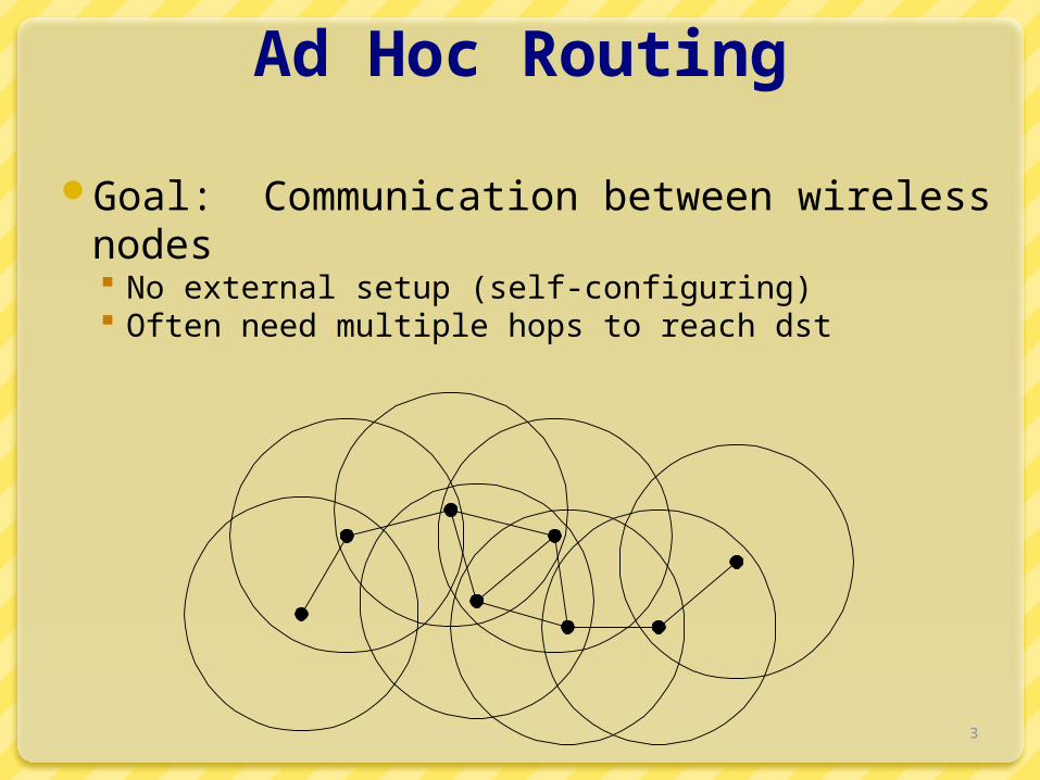
Goal: Communication between wireless nodes No external setup (self-configuring) Often need multiple hops to reach dst
4
Ad Hoc Routing
Create multi-hop connectivity among set of wireless, possibly moving, nodes
Mobile, wireless hosts act as forwarding nodes as well as end systems
Need routing protocol to find multi-hop paths Needs to be dynamic to adapt to new routes,
movement Interesting challenges related to interference and
power limitations Low consumption of memory, bandwidth, power Scalable with numbers of nodes Localized effects of link failure

5
Challenges and Variants
Poorly-defined “links” Probabilistic delivery, etc. Kind of n2 links
Time-varying link characteristicsNo oracle for configuration (no ground
truth configuration file of connectivity)Low bandwidth (relative to wired)Possibly mobilePossibly power-constrained

6
Problems Using DV or LS
DV protocols may form loops Very wasteful in wireless: bandwidth, power Loop avoidance sometimes complex
LS protocols: high storage and communication overhead
More links in wireless (e.g., clusters) - may be redundant higher protocol overhead
7
Problems Using DV or LS
Periodic updates waste power Tx sends portion of battery power into air Reception requires less power, but periodic updates
prevent mobile from “sleeping”Convergence may be slower in conventional
networks but must be fast in ad-hoc networks and be done without frequent updates
8
Proposed Protocols
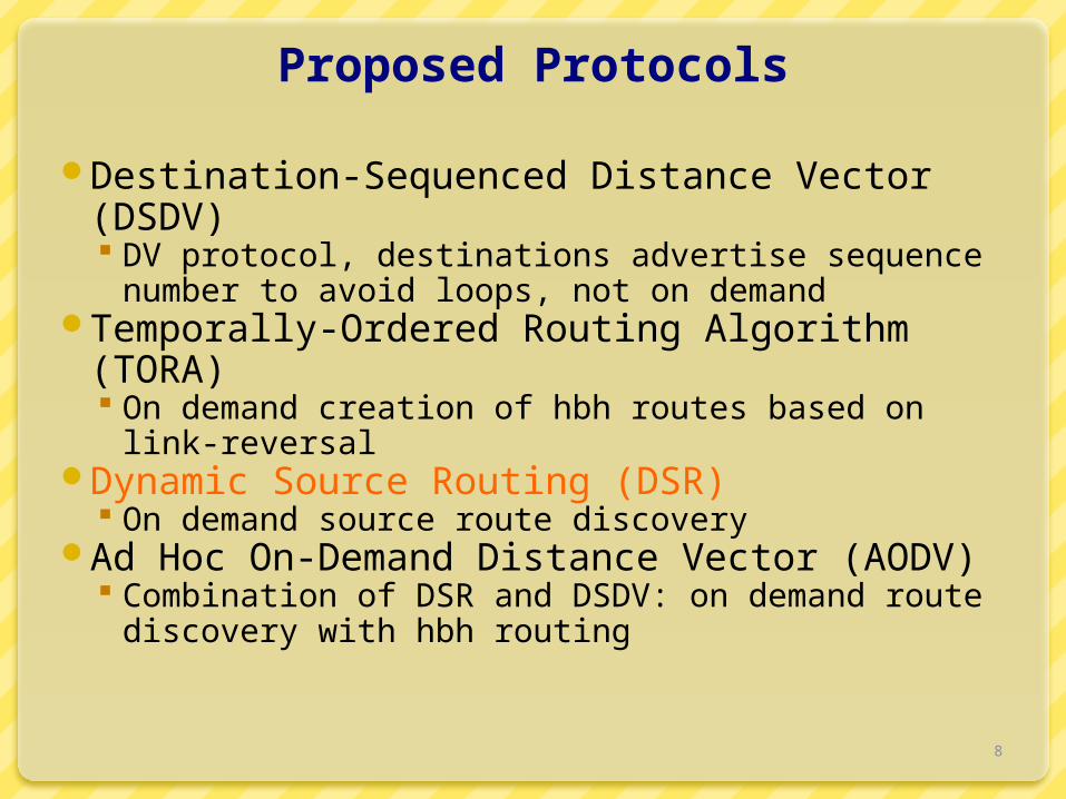
Destination-Sequenced Distance Vector (DSDV) DV protocol, destinations advertise sequence
number to avoid loops, not on demandTemporally-Ordered Routing Algorithm
(TORA) On demand creation of hbh routes based on link-
reversalDynamic Source Routing (DSR)
On demand source route discoveryAd Hoc On-Demand Distance Vector (AODV)
Combination of DSR and DSDV: on demand route discovery with hbh routing

9
DSR Concepts
Source routing No need to maintain up-to-date info at intermediate
nodesOn-demand route discovery
No need for periodic route advertisements
10
DSR Components
Route discovery The mechanism by which a sending node obtains a
route to destinationRoute maintenance
The mechanism by which a sending node detects that the network topology has changed and its route to destination is no longer valid
11
DSR Route Discovery
Route discovery - basic idea Source broadcasts route-request to Destination Each node forwards request by adding own address
and re-broadcasting Requests propagate outward until:
Target is found, or A node that has a route to Destination is found

12
C Broadcasts Route Request to F
A
SourceC
G H
DestinationF
E
D
BRoute Request

13
C Broadcasts Route Request to F
A
SourceC
G H
DestinationF
E
D
BRoute Request

14
H Responds to Route Request
A
SourceC
G H
DestinationF
E
D
B
G,H,F

15
C Transmits a Packet to F
A
SourceC
G H
DestinationF
E
D
B
FH,F
G,H,F

16
Forwarding Route Requests
A request is forwarded if: Node is not the destination Node not already listed in recorded source route Node has not seen request with same sequence
number IP TTL field may be used to limit scope
Destination copies route into a Route-reply packet and sends it back to Source

17
Route Cache
All source routes learned by a node are kept in Route Cache Reduces cost of route discovery
If intermediate node receives RR for destination and has entry for destination in route cache, it responds to RR and does not propagate RR further
Nodes overhearing RR/RP may insert routes in cache

18
Sending Data
Check cache for route to destinationIf route exists then
If reachable in one hop Send packet
Else insert routing header to destination and sendIf route does not exist, buffer packet and
initiate route discovery
19
Discussion
Source routing is good for on demand routes instead of a priori distribution
Route discovery protocol used to obtain routes on demand Caching used to minimize use of discovery
Periodic messages avoided

20
Overview
Ad Hoc Routing
Sensor Networks
Directed Diffusion
Aggregation TAG Synopsis Diffusion

21
Smart-Dust/Motes
First introduced in late 90’s by groups at UCB/UCLA/USC Published at Mobicom/SOSP conferences
Small, resource limited devices CPU, disk, power, bandwidth, etc.
Simple scalar sensors – temperature, motionSingle domain of deployment (e.g. farm,
battlefield, etc.) for a targeted task (find the tanks)
Ad-hoc wireless network
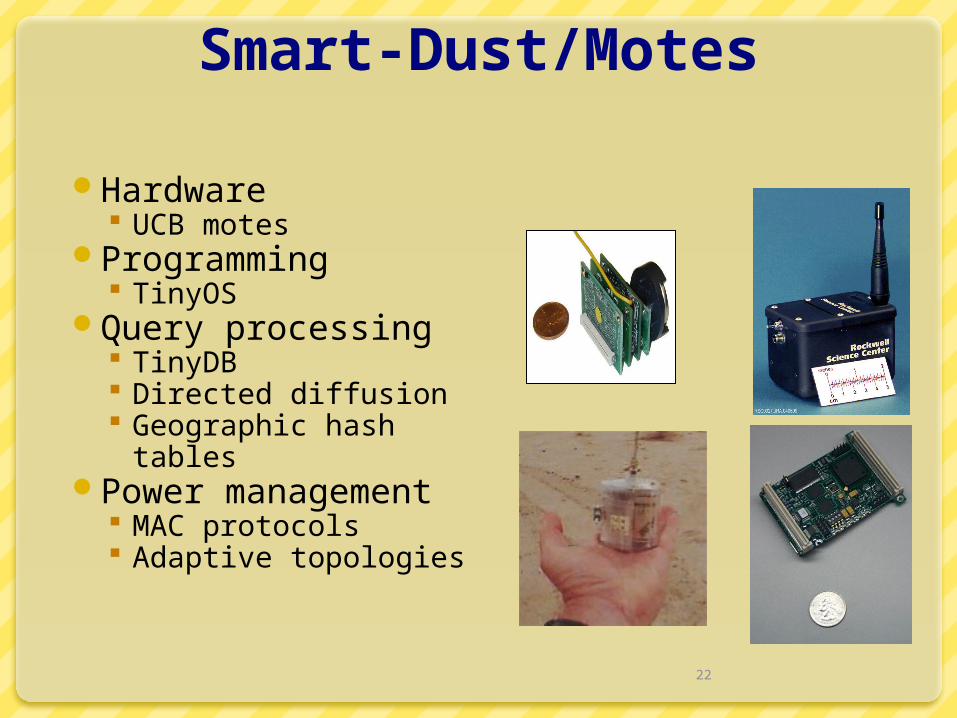
Smart-Dust/Motes
Hardware UCB motes
Programming TinyOS
Query processing TinyDB Directed diffusion Geographic hash
tablesPower management
MAC protocols Adaptive topologies
22

23
Berkeley Motes
Devices that incorporate communications, processing, sensors, and batteries into a small package
Atmel microcontroller with sensors and a communication unit RF transceiver, laser module,
or a corner cube reflector Temperature, light, humidity,
pressure, 3 axis magnetometers, 3 axis accelerometers

Berkeley Motes (Levis & Culler,
ASPLOS 02)
24
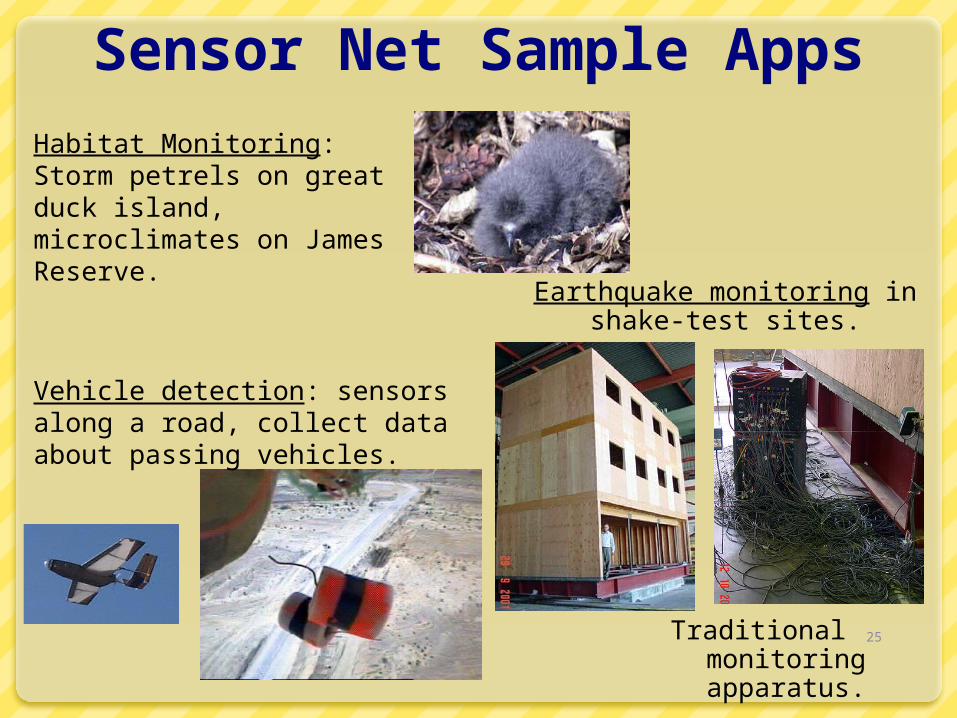
Sensor Net Sample Apps
25Traditional monitoring apparatus.
Earthquake monitoring in shake-test sites.
Vehicle detection: sensors along a road, collect data about passing vehicles.
Habitat Monitoring: Storm petrels on great duck island, microclimates on James Reserve.

26
Metric: Communication
Lifetime from one pair of AA batteries 2-3 days at full
power 6 months at 2%
duty cycleCommunication
dominates cost < few mS to
compute 30mS to send
message
Time v. Current Draw During Query Processing
0
5
10
15
20
0 0.5 1 1.5 2 2.5 3Time (s)
Cu
rre
nt
(mA
) Snoozing
Processing
Processingand Listening
Transmitting

27
Communication In Sensor Nets
Radio communication has high link-level losses typically about 20%
@ 5m
Ad-hoc neighbor discovery
Tree-based routing
A
B C
D
FE
28
Overview
Ad Hoc Routing
Sensor Networks
Directed Diffusion
Aggregation TAG Synopsis Diffusion

The long term goal
29
Disaster Response
Circulatory Net
Embed numerous distributed devices to monitor and interact with physical world: in work-spaces, hospitals, homes, vehicles, and “the environment” (water, soil, air…)
Network these devices so that they can coordinate to perform higher-level tasks.
Requires robust distributed systems of tens of thousands of devices.

Motivation
Properties of Sensor Networks Data centric, but not node centric Have no notion of central authority Are often resource constrained
Nodes are tied to physical locations, but: They may not know the topology They may fail or move arbitrarily
Problem: How can we get data from the sensors?
30

Directed Diffusion
Data centric – nodes are unimportantRequest driven:
Sinks place requests as interests Sources are eventually found and satisfy interests Intermediate nodes route data toward sinks
Localized repair and reinforcementMulti-path delivery for multiple sources,
sinks, and queries
31

Motivating Example
Sensor nodes are monitoring a flat space for animals
We are interested in receiving data for all 4-legged creatures seen in a rectangle
We want to specify the data rate
32

Interest and Event Naming
Query/interest:1. Type=four-legged animal2. Interval=20ms (event data rate)3. Duration=10 seconds (time to cache)4. Rect=[-100, 100, 200, 400]
Reply:1. Type=four-legged animal2. Instance = elephant3. Location = [125, 220]4. Intensity = 0.65. Confidence = 0.856. Timestamp = 01:20:40
Attribute-Value pairs, no advanced naming scheme
33

Diffusion (High Level)
Sinks broadcast interest to neighborsInterests are cached by neighborsGradients are set up pointing back to where
interests came from at low data rateOnce a sensor receives an interest, it routes
measurements along gradients
34

35
Illustrating Directed Diffusion
Sink
Source
Setting up gradients
Sink
Source
Sending data
Sink
Source
Recoveringfrom node failure
Sink
Source
Reinforcingstable path

Summary
Data Centric Sensors net is queried for specific data Source of data is irrelevant No sensor-specific query
Application Specific In-sensor processing to reduce data transmitted In-sensor caching
Localized Algorithms Maintain minimum local connectivity – save energy Achieve global objective through local coordination
Its gains due to aggregation and duplicate suppression may make it more viable than ad-hoc routing in sensor networks
36

37
Overview
Ad Hoc Routing
Sensor Networks
Directed Diffusion
Aggregation TAG Synopsis Diffusion

TAG Introduction Programming sensor nets is hard! Declarative queries are easy
Tiny Aggregation (TAG): In-network processing via declarative queries
In-network processing of aggregates Common data analysis operation Communication reducing
Operator dependent benefit Across nodes during same epoch
Exploit semantics improve efficiency!
Example: Vehicle tracking application: 2 weeks
for 2 students Vehicle tracking query: took 2 minutes
to write, worked just as well!
38
SELECT MAX(mag) FROM sensors WHERE mag > threshEPOCH DURATION 64ms
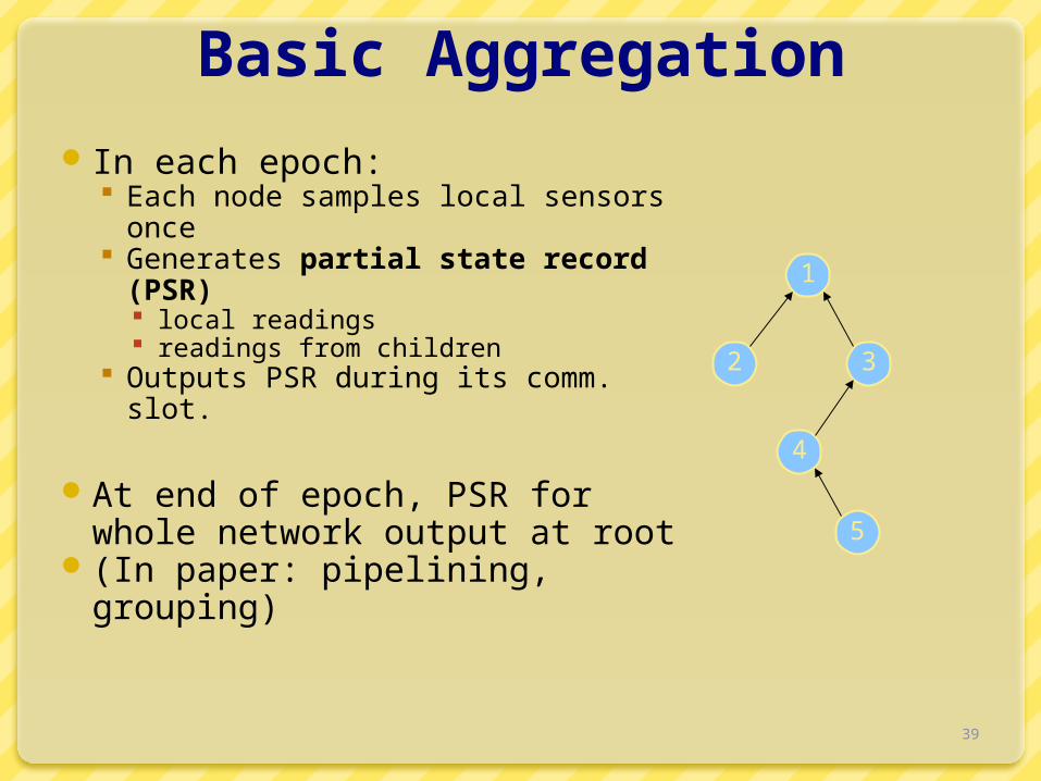
Basic Aggregation In each epoch:
Each node samples local sensors once Generates partial state record
(PSR) local readings readings from children
Outputs PSR during its comm. slot.
At end of epoch, PSR for whole network output at root
(In paper: pipelining, grouping)
39
1
2 3
4
5

40
Illustration: Aggregation
1 2 3 4 5
1 1
2
3
4
1
1
2 3
4
5
1
Sensor #
Slo
t #
Slot 1SELECT COUNT(*) FROM sensors

41
Illustration: Aggregation
1 2 3 4 5
1 1
2 2
3
4
1
1
2 3
4
5
2
Sensor #
Slo
t #
Slot 2SELECT COUNT(*) FROM sensors

42
Illustration: Aggregation
1 2 3 4 5
1 1
2 2
3 1 3
4
1
1
2 3
4
5
31
Sensor #
Slo
t #
Slot 3SELECT COUNT(*) FROM sensors

43
Illustration: Aggregation
1 2 3 4 5
1 1
2 2
3 1 3
4 5
1
1
2 3
4
5
5
Sensor #
Slo
t #
Slot 4SELECT COUNT(*) FROM sensors

44
Illustration: Aggregation
1 2 3 4 5
1 1
2 2
3 1 3
4 5
1 1
1
2 3
4
5
1
Sensor #
Slo
t #
Slot 1SELECT COUNT(*) FROM sensors

45
Types of Aggregates
SQL supports MIN, MAX, SUM, COUNT, AVERAGE
Any function can be computed via TAG
In network benefit for many operations E.g. Standard deviation, top/bottom N, spatial
union/intersection, histograms, etc. Compactness of PSR

Taxonomy of Aggregates
TAG insight: classify aggregates according to various functional properties Yields a general set of optimizations that can
automatically be applied
46
Property Examples AffectsPartial State MEDIAN : unbounded,
MAX : 1 recordEffectiveness of TAG
Duplicate Sensitivity
MIN : dup. insensitive,AVG : dup. sensitive
Routing Redundancy
Exemplary vs. Summary
MAX : exemplaryCOUNT: summary
Applicability of Sampling, Effect of Loss
Monotonic COUNT : monotonicAVG : non-monotonic
Hypothesis Testing, Snooping

47
Benefit of In-Network Processing
Total Bytes Xmitted vs. Aggregation Function
0
10000
20000
30000
40000
50000
60000
70000
80000
90000
100000
EXTERNAL MAX AVERAGE COUNT MEDIANAggregation Function
Tota
l Byt
es X
mitt
ed
Simulation Results
2500 Nodes
50x50 Grid
Depth = ~10
Neighbors = ~20
Some aggregates require dramatically more state!

48
Optimization: Channel Sharing (“Snooping”)
Insight: Shared channel enables optimizations
Suppress messages that won’t affect aggregate E.g., MAX Applies to all exemplary, monotonic aggregates

Optimization: Hypothesis Testing
Insight: Guess from root can be used for suppression E.g. ‘MIN < 50’ Works for monotonic & exemplary aggregates
Also summary, if imprecision allowed
How is hypothesis computed? Blind or statistically informed guess Observation over network subset
49

50
Optimization: Use Multiple Parents
For duplicate insensitive aggregatesOr aggregates that can be expressed as a
linear combination of parts Send (part of) aggregate to all parents
In just one message, via broadcast Decreases variance
A
B C
A
B C
A
B C
1
A
B C
A
B C
1/2 1/2

51
Overview
Ad Hoc Routing
Sensor Networks
Directed Diffusion
Aggregation TAG Synopsis Diffusion

52
Aggregation in Wireless Sensors
Aggregate data is often more important
1 1
31
1
37
1
2 1
103Count =
In-network aggregation over tree with unreliable communication
Not robust against node- or link-failures
Used by current systems, TinyDB [Madden et al. OSDI’02] Cougar [Bonnet et al. MDM’01]
10

53
Traditional Approach
Reliable communication E.g., RMST over Directed Diffusion [Stann’03]
High resource overhead 3x more energy consumption 3x more latency 25% less channel capacity
Not suitable for resource constrained sensors

54
Exploiting Broadcast Medium
Robust multi-path Energy-efficient
14
7
152
20 23
Count =
1
3
2
58
Double-counting Different ordering
Challenge: order and duplicate insensitivity(ODI)
10
Challenge

55
A Naïve ODI Algorithm
Goal: count the live sensors in the network
0 1 0 0 0 0 0 0 0 0 1 0
0 0 1 0 0 0 0 0 0 0 0 1
id Bit vector

56
Synopsis Diffusion (SenSys’04)
Goal: count the live sensors in the network
0 1 0 0 0 0 0 0 0 0 1 0
0 0 1 0 0 0 0 0 0 0 0 1
id Bit vector
0 1 0 0 0 0 BooleanOR
0 1 0 0 1 0
0 1 1 0 0 0
0 1 0 0 0 0 0 1 0 0 1 0
0 1 1 0 1 0
0 1 0 0 1 0
0 1 0 0 1 1
0 1 1 0 1 1 Count 1 bits
4
Synopsis should be small
Approximate COUNT algorithm: logarithmic size bit vector
Challenge

Synopsis Diffusion over Rings
A node is in ring i if it is i hops away from the base-station
Broadcasts by nodes in ring i are received by neighbors in ring i-1
Each node transmits once = optimal energy cost (same as Tree)
57
Ring 2

58
Evaluation
Approximate COUNT with Synopsis Diffusion
Scheme Energy
Tree 41.8 mJ
Syn. Diff. 42.1 mJ
0
0.25
0.5
0.75
1
0 0.25 0.5 0.75 1
Loss Rate
RM
S E
rro
r
Tree Syn. Diff.
More robust than Tree
Almost as energy efficient as Tree
Per node energy
Typicalloss rates