Kyoto University, Graduate School of Economics Research Project Center Discussion Paper Series

Electricity demand response in Japan:

Experimental evidence from a residential photovoltaic generation system

Takanori Ida, Kayo Murakami , Makoto Tanaka

Discussion Paper No. E-15-006

Research Project Center Graduate School of Economics

Kyoto University Yoshida-Hommachi, Sakyo-ku Kyoto City, 606-8501, Japan

August, 2015

1

Electricity demand response in Japan: Experimental evidence from a residential photovoltaic generation system Takanori Ida1 Graduate School of Economics, Kyoto University, Japan Kayo Murakami2 Chikushi Jogakuen University, Japan Makoto Tanaka3 National Graduate Institute for Policy Studies, Japan Abstract: We report on a randomized controlled trial used to examine the effect of dynamic pricing when applied to households with rooftop photovoltaic (PV) power-generation systems. Using high-frequency data on household-level electricity use, PV generation, purchases, and sales, we find that critical peak pricing induced significant usage reductions of 3-4% among households with PV systems, a quarter of the effect size seen among average households without solar PV systems. In addition, we investigate the influence of the amount of PV power generated on treatment effects and the potential heterogeneity caused by participating households’ attributes. This is the first large-scale field experiment evaluating the demand response of households with PV generation capabilities. JEL classification codes: D1 - Household Behavior; Q4 - Energy Keywords: randomized controlled trial, field experiment, photovoltaic generation, dynamic pricing

1 Yoshida, Sakyo-ku, Kyoto 606-8501, Japan.

E-mail: ida@econ.kyoto-u.ac.jp 2 2-12-1 Ishizaga, Dazaifu City, Fukuoka 818-0192, Japan.

E-mail: murakamikayo@gmail.com 3 7-22-1 Roppongi, Minato-ku, Tokyo 106-8677, Japan.

E-mail: mtanaka@grips.ac.jp

2

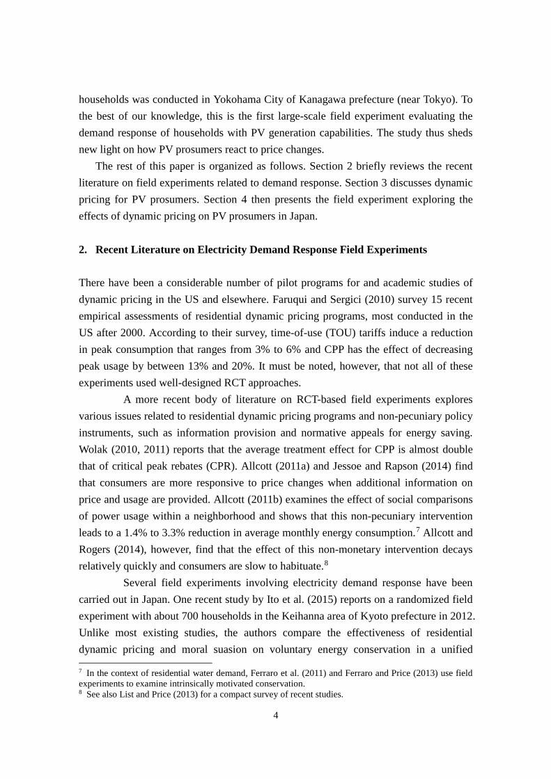
1. Introduction In March 2011, the Great East Japan Earthquake and subsequent tsunami seriously damaged the Fukushima Daiichi Nuclear Power Station. Prior to these disasters in 2010, 29% of Japan’s electricity was supplied by nuclear energy, while the shares provided by fossil fuels and renewable energy sources were, respectively, 62% (liquefied natural gas (LNG), 29%; coal, 25%; oil, 8%) and 10% (hydropower, 9%; other renewables, 1%). This had changed widely by 2013, when nuclear generation accounted for only 1% of total power supply and the share obtained from fossil fuel sources had increased significantly to 88% (LNG, 43%; coal, 30%; oil, 15%), while that from renewables remained at 11% (hydropower, 9%; other renewables, 2%).4

The dramatic fall in nuclear power generation was due to a suspension of operations after the disasters. The nuclear power plants that were not directly damaged by the earthquake were gradually shut down for scheduled maintenance. Finally in September 2013, the last two nuclear reactors were shut down; thus, all of Japan’s 48 reactors were suspended until given approval to restart from the Nuclear Regulation Authority (NRA). Almost half of those reactors were undergoing NRA safety assessments as of early 2015, but their restarted operation will not be fully approved for a long time because of an envisaged six-month (or much longer) timeline for rigorously assessing each case. In addition, local governments’ agreement and local communities’ acceptance are necessary for the nuclear reactors to resume operations.

As a result, Japan has been faced with challenges in restructuring its energy and environment systems to achieve both short- and long-run sustainability. The amount of power supplied by fossil fuel sources has dramatically increased, pushing up import costs of these fuels and hence raising power generation costs. The cost of nuclear power generation has also risen because of the stricter safety measures required for operation under the NRA’s new safety standards. On the other hand, there is pressure to reduce greenhouse gas emissions from the power sector to combat climate change.

In recent years, renewable energy and demand-side resources have been key issues as Japan (and the US, EU, and many other countries) attempts to tackle the dilemma of securing its energy supply without further increasing its environmental footprint; these challenges have become particularly acute after the energy crisis. The Japanese government seeks to double the share of renewable energy in national consumption to reach 24% in 2030 while increasing nuclear power to about 20%, still

4 The Federation of Electric Power Companies (FEPC) reports the composition of annual electricity generated in Japan (http://www.fepc.or.jp/about_us/pr/pdf/kaiken_s1_20140523.pdf).

3

below the pre-Fukushima level. 5 Although there is little scope for increasing hydroelectric power (9%) in Japan, the government envisages the share of solar photovoltaic (PV) power rising to 7% in 2030, followed by 5% from biomass, 2% from wind power, and 1% from geothermal power.6 Specifically, PV power generation capacity is expected to increase from 13GW in 2013 to 64GW in 2030, a fivefold increase.

Considering demand-side management, the Japanese government expects 17% energy savings compared to the reference case. One key target is to improve efficiency in residential energy management. Most Japanese residential consumers are currently charged flat-rate tariffs for electricity using conventional analog electric meters, but the government plans to install digital smart meters in all households (about 50 million) in Japan by 2024. Along with smart meters and possibly home energy management system (HEMS), dynamic pricing schemes, such as critical peak pricing (CPP) and real time pricing (RTP), are expected to induce residential consumers to use electricity more efficiently.

The past decade has seen a growing body of literature reporting on field experiments with electricity demand response; we will briefly survey these in the next section, with a focus on the Japanese case. However, we are not aware of any study documenting large-scale field experiments investigating demand response among households with rooftop PV generation systems. A household with a PV generation system can be regarded as a “prosumer” (i.e., a combination of a producer and a consumer). A PV prosumer can generate electricity using a solar panel and sell it to power companies while also consuming electricity in the home. This prosumer can be a net buyer or seller of electricity, depending on weather conditions and the solar panel’s capacity. As discussed above, significant increases in both PV generation and demand-side resources are expected by 2030 in Japan. Given this, it is useful to understand the impact of dynamic pricing on PV prosumers’ behavior.

In this paper, we use a randomized controlled trial (RCT) to examine the effect of dynamic pricing, specifically CPP, when applied to households with rooftop PV generation systems. In 2013, a randomized field experiment with about 1,200

5 Murakami et al. (2015) examine consumers’ willingness to pay for nuclear and renewable electricity as two alternatives to fossil fuel sources. Based on a choice experiment using consumer-stated preferences, they demonstrate that Japanese consumers have a strong aversion to nuclear energy but a strong acceptance of emissions reductions through the use of renewable energy sources. 6 In April 2015, Japan’s Ministry of Economy, Trade and Industry (METI) announced a plan for the country’s energy portfolio in 2030 (http://www.enecho.meti.go.jp/committee/council/basic_policy_subcommittee/mitoshi/008/pdf/008_07.pdf).

4

households was conducted in Yokohama City of Kanagawa prefecture (near Tokyo). To the best of our knowledge, this is the first large-scale field experiment evaluating the demand response of households with PV generation capabilities. The study thus sheds new light on how PV prosumers react to price changes.

The rest of this paper is organized as follows. Section 2 briefly reviews the recent literature on field experiments related to demand response. Section 3 discusses dynamic pricing for PV prosumers. Section 4 then presents the field experiment exploring the effects of dynamic pricing on PV prosumers in Japan.

2. Recent Literature on Electricity Demand Response Field Experiments There have been a considerable number of pilot programs for and academic studies of dynamic pricing in the US and elsewhere. Faruqui and Sergici (2010) survey 15 recent empirical assessments of residential dynamic pricing programs, most conducted in the US after 2000. According to their survey, time-of-use (TOU) tariffs induce a reduction in peak consumption that ranges from 3% to 6% and CPP has the effect of decreasing peak usage by between 13% and 20%. It must be noted, however, that not all of these experiments used well-designed RCT approaches.

A more recent body of literature on RCT-based field experiments explores various issues related to residential dynamic pricing programs and non-pecuniary policy instruments, such as information provision and normative appeals for energy saving. Wolak (2010, 2011) reports that the average treatment effect for CPP is almost double that of critical peak rebates (CPR). Allcott (2011a) and Jessoe and Rapson (2014) find that consumers are more responsive to price changes when additional information on price and usage are provided. Allcott (2011b) examines the effect of social comparisons of power usage within a neighborhood and shows that this non-pecuniary intervention leads to a 1.4% to 3.3% reduction in average monthly energy consumption.7 Allcott and Rogers (2014), however, find that the effect of this non-monetary intervention decays relatively quickly and consumers are slow to habituate.8

Several field experiments involving electricity demand response have been carried out in Japan. One recent study by Ito et al. (2015) reports on a randomized field experiment with about 700 households in the Keihanna area of Kyoto prefecture in 2012. Unlike most existing studies, the authors compare the effectiveness of residential dynamic pricing and moral suasion on voluntary energy conservation in a unified 7 In the context of residential water demand, Ferraro et al. (2011) and Ferraro and Price (2013) use field experiments to examine intrinsically motivated conservation. 8 See also List and Price (2013) for a compact survey of recent studies.

5

field-experimental framework. They report that the average treatment effects of CPP and moral suasion without economic incentives are about 16% and 3%, respectively, which are consistent with the results of existing studies.9 Moreover, they compare the persistence of treatment effects between monetary and non-monetary interventions. The moral suasion group shows a usage reduction of 8% during the first few treatment days, but the effect quickly diminishes to zero with repeated interventions. In contrast, the effect of CPP is much larger and more persistent over repeated interventions. The authors further find significant habit formation among the CPP group but no habit formation for the moral suasion group after the final intervention. Their follow-up survey data indicates that most of the persistent changes likely originate in behavioral lifestyle changes (e.g., more efficient use of air conditioners) rather than investment in durable goods.

3. Dynamic Pricing for PV Prosumers Several countries have already adopted feed-in tariff (FIT) policies to encourage adoption of renewable energy sources. In a typical FIT scheme, a household with a PV system receives a set rate for all of the electricity it generates, regardless of whether it consumes part of it within the house. The household continues to pay the retail price for all electricity that it consumes at home, like a typical electric utility customer. Under this typical scheme, it is straightforward to apply dynamic pricing to the retail price for power purchases in order to induce a demand response.

Under another type of FIT scheme, a household receives a set rate only for the “surplus” electricity it provides to the grid (i.e., PV generation – in-home consumption). Even under this scheme, dynamic pricing could be applied to the retail purchase price at times when the household is a net electricity buyer (e.g., during cloudy weather). However, when the household is a net seller (e.g., during sunny weather), standard dynamic pricing cannot be used because the household does not purchase electricity during that period. One natural extension of dynamic pricing to apply to this case would be to raise the sale price for the surplus electricity above the set FIT rate. Then, even a net seller household would have an incentive to reduce its home power consumption in order to sell more PV electricity at a higher price (see Fig. 1).

9 In their study, the baseline price was 25 cents/kWh and the CPP group experienced three different levels of critical peak prices: 65, 85, and 105 cents/kWh. The size of the reduction in peak consumption monotonically increased as customers were charged higher prices. This price schedule can be called “variable CPP.” The same authors also applied variable CPP to a field experiment in Kitakyushu City, Japan and obtained consistent results for demand response.

6

<Insert Fig. 1>

Japan uses the latter FIT scheme form for its residential solar PV systems: the

FIT rate is set for surplus electricity provided by households.10 At the time of our experiment in Yokohama City, the set FIT rate was 42 cents/kWh, while the retail purchase price of electricity was about 25 cents/kWh. In our experiment, we applied variable CPP with two different price levels: 60 and 100 cents/kWh. The surplus electricity selling price faced by a net seller and the retail purchase price faced by a net buyer are raised to the same price level (60 or 100 cents/kWh) to ensure the same marginal incentives apply to every PV household. 4. The Randomized Field Experiment

The field experiment reported here was conducted on PV prosumers in

Yokohama, Kanagawa Prefecture in the summer of 2013. The experiment was implemented in collaboration with METI, The New Energy Promotion Council (NEPC), the city of Yokohama, Tokyo Electric Power Company (TEPCO), Toshiba, Ltd., and Panasonic, Ltd. Smart meters recording households’ electricity consumption at 30-minute intervals and HEMS recording PV generation at 30-minute intervals were installed in the 1,202 households who own rooftop PV generation systems and reside in the city of Yokohama. In addition, the total amounts of electricity purchased and sold were observed using PV monitoring devices in each household. We then used an RCT approach to examine the effect of CPP tariffs. This section describes our experimental design, data, treatment, hypotheses, and results. 4.1 Experimental Design and Data

We recruited participants using a public relations campaign publicizing the field experiment. To engage as broad a set of households as possible, we provided generous participation rewards, including free installation of a smart meter and a HEMS and a participation reward of $100 per year. Information on household consumption and real-time prices were always available online for participants to access. In the end, 1,202 customers confirmed their participation. In an RCT, individuals are randomly assigned to the treatment and control groups to avoid selection bias (Duflo et al. 2007).

10 METI launched the current FIT scheme in 2012 (http://www.meti.go.jp/english/policy/energy_environment/renewable/).

7

We thus randomly assigned the 1,202 households to one of three groups: control (C), treatment 1 (T1), and treatment 2 (T2). Figure 2 shows the experimental design and group assignment; the groups are described as follows.

1. Control Group (C): 353 households were assigned to the control group. Of these, 32 were excluded because of changing to another plan or missing data due to technical troubles with the HEMS. Of the remaining participants, 164 households had made contracts using the Yokohama flat rate and 157 had made contracts using the TOU rate as the regular price. This group received no additional treatment.

2. Treatment Group 1 (T1): 427 households were assigned to this treatment group. Of these, 26 were excluded because of changing to another plan or missing data due to technical troubles with the HEMS. Of the remaining participants, 211 households had made contracts using the Yokohama flat rate and 190 had made contracts using the TOU rate as the regular price. In addition, this group received the “CPP 60 treatment,” as described below, on treatment days.

3. Treatment Group 2 (T2): 422 households were assigned to this treatment group. Of these, 31 households were excluded because of changing to another plan or missing data due to technical troubles with the HEMS. Of the remaining participants, 210 households had made contracts using the Yokohama flat rate and 181 had made contracts using the TOU rate as the regular price. In addition, this group received the “CPP 100 treatment,” as described below, on treatment days.

<Insert Fig. 2>

The study thus uses high-frequency data on household electricity usage, PV

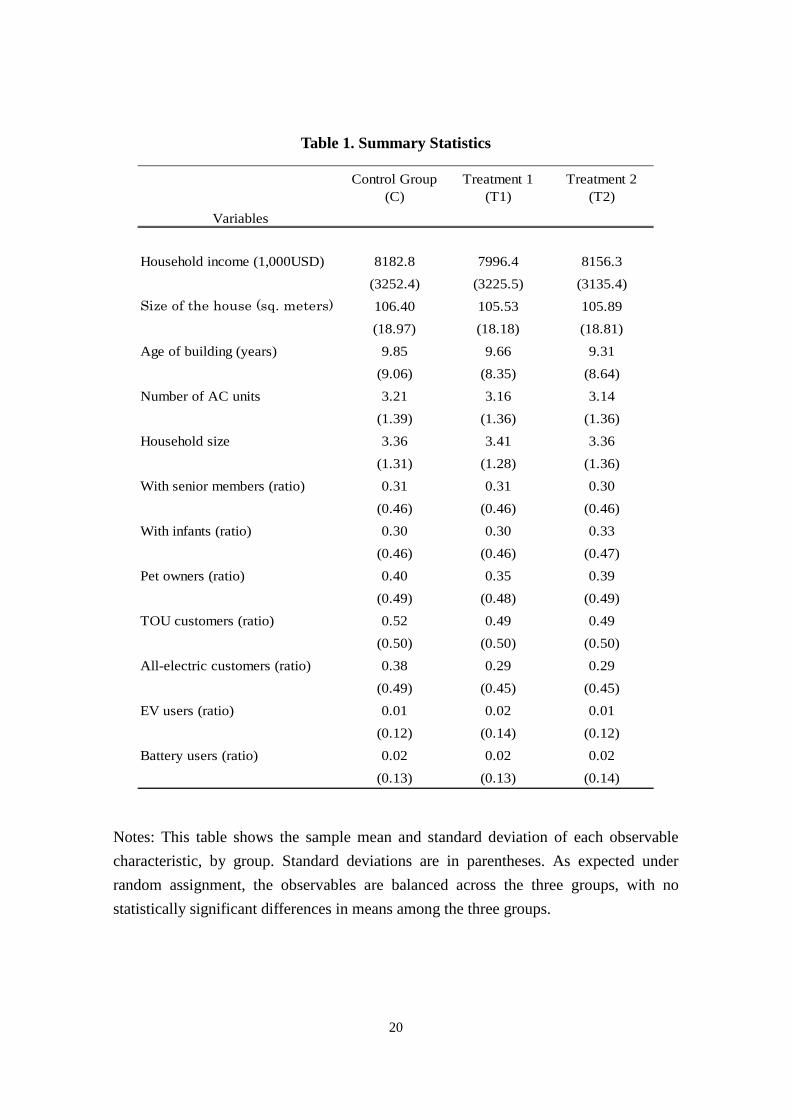
generation, purchases, and sales for 68 days from June 1 to September 6, 2013. We conducted a survey prior to treatment assignment to collect demographic information. Table 1 shows summary statistics for the three groups. As expected given the random assignment of the groups, none of the means are statistically different among the three groups.

<Insert Table 1>

8

4.2 Treatment In this experiment, we explore the effect of the CPP tariff on cutting peak

power demand (henceforth “the peak-cut effect”). A fundamental economic inefficiency in electricity markets is that electricity consumers generally do not pay prices that reflect the high marginal cost of generating electricity during peak demand hours (Borenstein 2002; Joskow 2012). A CPP tariff is a variable electricity rate program that reflects the marginal power generation costs in different time periods; a unit cost several times higher than the normal electricity rate is used during these time periods on designated high demand days. In this experiment, electricity rates were set to 60 or 100 cents/kWh from 1:00 to 4:00 PM (the system peak in Japan) on the treatment days, in contrast to the standard flat rate of 25 cents/kWh for Yokohama customers.

Figure 3 shows the dynamic electricity-pricing schedule used in each group. First, within the control group, a constant price of 25 cents/kWh was applied for participants using a flat-rate system as their regular rate, while a price of 38 cents/kWh was applied during peak time periods for participants using a TOU rate system as their regular rate. A rate of either 60 or 100 cents/kWh was applied to participants assigned to the treatment groups during peak time periods on treatment days.

＜Insert Figure 3a＞ ＜Insert Figure 3b＞

In this experiment, all customers had rooftop PV generation systems installed.

Figure 4 shows the average amount of PV generation in each time period and the share of households that sold more electricity than they bought (that is, the net sellers) for the selected time periods. Many households produced surplus electricity during the treatment period (1:00 to 4:00 PM, the peak time period) on treatment days, with the majority being net electricity sellers. While the purchase price set by the electric company based on the FIT at the time was 42 cents/kWh across the board, the rate for electricity sold during peak time periods on treatment days was set to 60 or 100 cents/kWh. If customers consumed less power than they generated during peak time periods, they were paid in the form of rebates for the surplus electricity sold to the electric company. This can be referred to as a CPR tariff: an electricity rate system in which, rather than raising electricity rates during peak time periods, customers are given rebates for bringing their consumption below a predetermined electricity consumption baseline. In other words, the experiment was set up so that, when customers reduced consumption during peak time periods, a CPP program using the electricity purchase

9

price was applied if electricity consumed exceeded self-generated electricity, while a CPR program using the electricity sale price was applied when electricity consumed was less than self-generated electricity.

Accordingly, the price incentives (price changes) applied to the treatment groups on treatment days are as follows. Participants using the default flat-rate plan had price incentives of 35 or 75 cents/kWh when purchasing electricity and 18 or 58 cents/kWh when selling electricity. Participants using the default TOU rate plan had price incentives of 22 or 62 cents/kWh when purchasing electricity and 18 or 58 cents/kWh when selling electricity. Therefore, while participants in both rate plans encountered the same incentives when selling electricity, different incentives based on the plan were applied when purchasing electricity. We predicted that households participating in the flat-rate plan would show a larger marginal change in demand and a comparatively larger peak-cut effect.11

＜Insert Figure 4＞

We informed customers about how they would be receiving the treatment. First, the treatment hours were predetermined (1:00 to 4:00 PM). Second, we defined the treatment days as follows. A treatment day had to be a weekday upon which the day-ahead maximum temperature forecast exceeded 31°C (88°F). Some adjustments were made in order to secure sufficient data about treatment days, such as by planning treatment days when high demand was expected based on weather even if the expected maximum temperature was between 29°C (86°F) and 30°C (87°F). As a result, the treatment groups experienced 14 treatment days during the period. Customers were told that they would receive day-ahead and same-day notices about treatment days via e-mail. 4.3 Hypotheses

The field experiment is used to test several hypotheses. First, we estimate the treatment effect of a CPP tariff targeting PV prosumers and investigate whether the effect differs from a program targeting average households. Second, we study whether customers respond to different price incentives—i.e., if they respond differently to

11 To determine whether a participant is in a state of buying or selling electricity, it is necessary each time to access the online HEMS information and compare electricity consumption and self-generated electricity. As such, it is unlikely that most customers were able to correctly determine whether they were buying or selling electricity at any given moment; this may weaken the asymmetric effect of incentives for buying and selling.

10

marginal prices differing from the separate rates (60 or 100 cents) set in the CPP tariffs or if they simply respond to a pricing event. Furthermore, we investigate whether treatment effects differ based on the rate plan (flat or TOU) used to define the customer’s regular rate. As described above, customers enrolled in each plan encounter price changes that differ on treatment days; the implications of the results for policymakers differ based on whether customers respond differently to these different incentives. Third, in order to study how possession of a PV system—a feature of the experiment—influences treatment effects, we estimate the influence of PV power generation amounts on treatment effects. Lastly, to investigate heterogeneity in treatment, we estimate the influence of participating households’ attributes on the treatment effects. 4.4 Empirical Analysis and Results

We estimate the peak-cut effects using the following panel data regressions controlling for household and time fixed effects.

ln 𝑦𝑦𝑖𝑖𝑖𝑖 = ∑ 𝛼𝛼𝑔𝑔 ∙ 𝐼𝐼𝑖𝑖𝑖𝑖𝑔𝑔

𝑔𝑔∈{𝐶𝐶𝐶𝐶𝐶𝐶60,𝐶𝐶𝐶𝐶𝐶𝐶100} + 𝜃𝜃𝑖𝑖 + 𝜆𝜆𝑖𝑖 + 𝜀𝜀𝑖𝑖𝑖𝑖 (1)

where ln 𝑦𝑦𝑖𝑖𝑖𝑖 is the natural log of electricity consumption of household 𝑖𝑖 during a 30-minute interval 𝑡𝑡12

P. 𝐼𝐼𝑖𝑖𝑖𝑖𝑔𝑔 equals 1 if household 𝑖𝑖 is in the treatment group 𝑔𝑔 with

𝑔𝑔 ∈ {𝐶𝐶𝐶𝐶𝐶𝐶60, 𝐶𝐶𝐶𝐶𝐶𝐶100} and if a dynamic pricing event occurs for 𝑖𝑖 in 𝑡𝑡. Here, “𝐶𝐶𝐶𝐶𝐶𝐶60” and “𝐶𝐶𝐶𝐶𝐶𝐶100” denote the CPP 60 and CPP 100 groups, respectively. 𝜃𝜃𝑖𝑖 denotes a household fixed effect that controls for persistent differences in consumption across households, and 𝜆𝜆𝑖𝑖 denotes a time fixed effect for 30-minute interval 𝑡𝑡 that accounts for weather and other shocks specific to 𝑡𝑡. 𝜀𝜀𝑖𝑖𝑖𝑖 is an unobserved, mean-zero error term controlling for serial correlation and heteroscedasticity.

Table 2 shows the results for the peak-cut effect (percentage), estimated using verified data from summer 2013 (weekdays only). Each treatment group reduced its consumption of electricity during peak time periods with a high level of statistical significance. Recall that the baseline marginal price was 25 cents/kWh and that the treatment groups experienced the two critical peak prices: 60 and 100 cents/kWh. The results in Table 2 indicate that consumption reductions monotonically increase when customers are charged higher marginal prices. As shown in column (1), for example, critical peak prices of 60 and 100 cents/kWh produced reductions in usage of 2.7% and 12 We use the natural log of usage for the dependent variable so that we can interpret the treatment effects in approximate percentage terms. The treatment effects in exact percentage terms can be obtained by 𝑒𝑒𝑒𝑒𝑒𝑒(𝛼𝛼𝑔𝑔) − 1.

11

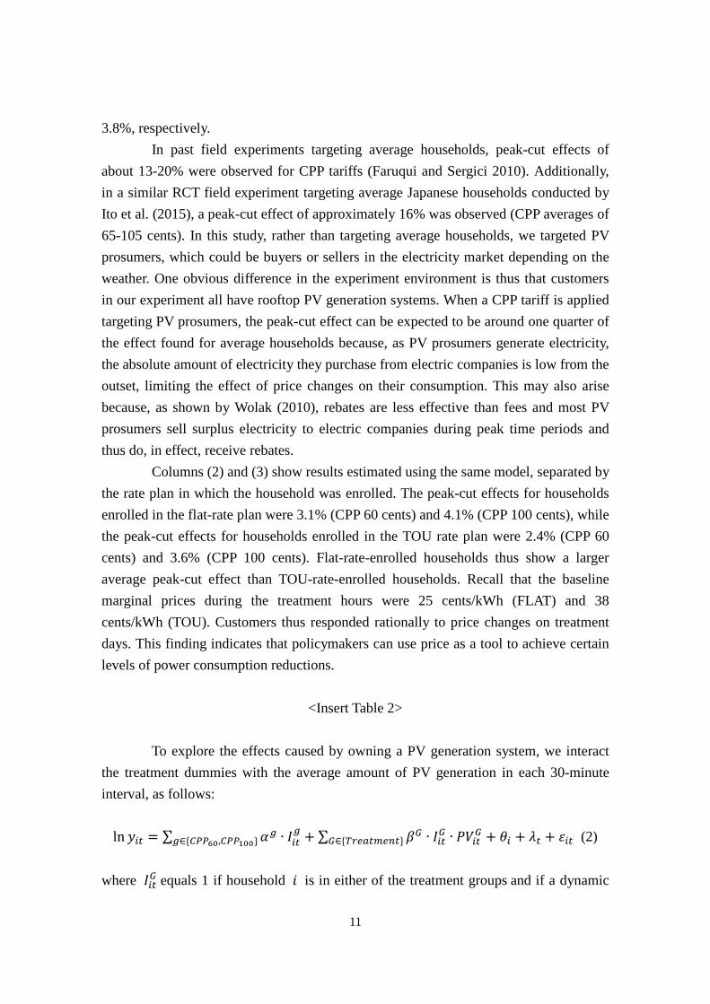
3.8%, respectively. In past field experiments targeting average households, peak-cut effects of

about 13-20% were observed for CPP tariffs (Faruqui and Sergici 2010). Additionally, in a similar RCT field experiment targeting average Japanese households conducted by Ito et al. (2015), a peak-cut effect of approximately 16% was observed (CPP averages of 65-105 cents). In this study, rather than targeting average households, we targeted PV prosumers, which could be buyers or sellers in the electricity market depending on the weather. One obvious difference in the experiment environment is thus that customers in our experiment all have rooftop PV generation systems. When a CPP tariff is applied targeting PV prosumers, the peak-cut effect can be expected to be around one quarter of the effect found for average households because, as PV prosumers generate electricity, the absolute amount of electricity they purchase from electric companies is low from the outset, limiting the effect of price changes on their consumption. This may also arise because, as shown by Wolak (2010), rebates are less effective than fees and most PV prosumers sell surplus electricity to electric companies during peak time periods and thus do, in effect, receive rebates.

Columns (2) and (3) show results estimated using the same model, separated by the rate plan in which the household was enrolled. The peak-cut effects for households enrolled in the flat-rate plan were 3.1% (CPP 60 cents) and 4.1% (CPP 100 cents), while the peak-cut effects for households enrolled in the TOU rate plan were 2.4% (CPP 60 cents) and 3.6% (CPP 100 cents). Flat-rate-enrolled households thus show a larger average peak-cut effect than TOU-rate-enrolled households. Recall that the baseline marginal prices during the treatment hours were 25 cents/kWh (FLAT) and 38 cents/kWh (TOU). Customers thus responded rationally to price changes on treatment days. This finding indicates that policymakers can use price as a tool to achieve certain levels of power consumption reductions.

<Insert Table 2>

To explore the effects caused by owning a PV generation system, we interact the treatment dummies with the average amount of PV generation in each 30-minute interval, as follows:

ln 𝑦𝑦𝑖𝑖𝑖𝑖 = ∑ 𝛼𝛼𝑔𝑔 ∙ 𝐼𝐼𝑖𝑖𝑖𝑖𝑔𝑔

𝑔𝑔∈{𝐶𝐶𝐶𝐶𝐶𝐶60,𝐶𝐶𝐶𝐶𝐶𝐶100} + ∑ 𝛽𝛽𝐺𝐺 ∙ 𝐼𝐼𝑖𝑖𝑖𝑖𝐺𝐺 ∙ 𝐶𝐶𝑃𝑃𝑖𝑖𝑖𝑖𝐺𝐺𝐺𝐺∈{𝑇𝑇𝑇𝑇𝑇𝑇𝑇𝑇𝑖𝑖𝑇𝑇𝑇𝑇𝑇𝑇𝑖𝑖} + 𝜃𝜃𝑖𝑖 + 𝜆𝜆𝑖𝑖 + 𝜀𝜀𝑖𝑖𝑖𝑖 (2) where 𝐼𝐼𝑖𝑖𝑖𝑖𝐺𝐺 equals 1 if household 𝑖𝑖 is in either of the treatment groups and if a dynamic

12

pricing event occurs for 𝑖𝑖 in period 𝑡𝑡, and 𝐶𝐶𝑃𝑃𝑖𝑖𝑖𝑖𝐺𝐺 denotes the amount of PV generation by household 𝑖𝑖 in period 𝑡𝑡. Therefore, 𝛽𝛽𝐺𝐺 is a parameter denoting the effect of PV generation on electricity usage. When 𝛽𝛽𝐺𝐺 is positive (negative), this can be interpreted as electricity consumption being high (low) during time periods when a household’s PV generation is high and the peak-cut effect being small (large).

Table 3 shows the results of estimating regressions that include interaction terms for average PV generation. The sign on 𝛽𝛽𝐺𝐺 is positive, indicating that the higher a household’s PV generation amount, the smaller the peak-cut effect. As shown in Figure 4, during time periods of high PV generation, most PV prosumers produce electricity surpluses and are net electricity sellers. This can be interpreted in two ways. First, the peak-cut effect is small when the net selling ratio is high (that is, framed as a gain) and, conversely, the peak-cut effect is large when the net buying ratio is high (that is, framed as a loss).13 Second, recalling that under both rate plans the price incentives are stronger for purchasing electricity, our findings can also be interpreted as stemming from different marginal price changes. We cannot differentiate these two reasonable interpretations based on our estimation results.

<Insert Table 3>

To explore the effects caused by potential heterogeneity in the CPP tariff treatment effects, we interact the treatment dummies with several household characteristics, as shown in Table 1. ln 𝑦𝑦𝑖𝑖𝑖𝑖 = ∑ 𝛼𝛼𝑔𝑔 ∙ 𝐼𝐼𝑖𝑖𝑖𝑖

𝑔𝑔𝑔𝑔∈{𝐶𝐶𝐶𝐶𝐶𝐶60,𝐶𝐶𝐶𝐶𝐶𝐶100} + ∑ 𝛽𝛽𝐺𝐺 ∙ 𝐼𝐼𝑖𝑖𝑖𝑖𝐺𝐺 ∙ 𝐶𝐶𝑃𝑃𝑖𝑖𝑖𝑖𝐺𝐺𝐺𝐺∈{𝑇𝑇𝑇𝑇𝑇𝑇𝑇𝑇𝑖𝑖𝑇𝑇𝑇𝑇𝑇𝑇𝑖𝑖} + ∑ 𝛾𝛾𝐺𝐺 ∙𝐺𝐺∈{𝑇𝑇𝑇𝑇𝑇𝑇𝑇𝑇𝑖𝑖𝑇𝑇𝑇𝑇𝑇𝑇𝑖𝑖}

𝐼𝐼𝑖𝑖𝑖𝑖𝐺𝐺 ∙ 𝐻𝐻𝑖𝑖𝐺𝐺 + 𝜃𝜃𝑖𝑖 + 𝜆𝜆𝑖𝑖 + 𝜀𝜀𝑖𝑖𝑖𝑖 (3) Because 𝐻𝐻𝑖𝑖𝐺𝐺 denotes household 𝑖𝑖’s characteristics, as shown in Table 1, 𝛾𝛾𝐺𝐺 indicates the effects of their heterogeneity.

Table 4 shows the results of estimating regressions including such interaction terms for several household characteristics. We find consistent relationships between treatment effects and income and other household characteristics. The CPP treatment

13 Kahneman and Tversky (1979), Kahneman et al. (1991), and Tversky and Kahneman (1991) are the representative papers on reference-dependent preferences; their results demonstrate that individual behavior is consistent with the notion of loss aversion. For recent field experiments testing framing effects in the context of losses versus gains, see Hossain and List (2012), Fryer et al. (2012), Ida and Wang (2014).

13

effect is lower for higher-income households than for lower-income households.14 Similarly, the CPP treatment effect is larger for households with physically larger houses and smaller household sizes. In addition, the CPP treatment effect is smaller for households including those over sixty years old and electric vehicle (EV) owners.

<Insert Table 4> 5. Conclusion In this paper, we conducted a large-scale field experiment to evaluate the impact of dynamic pricing on the behavior of PV prosumers. Using high-frequency data on electricity use, PV generation, purchases, and sales at the household level, we found that CPP tariffs induced significant usage reductions of 3-4% among PV prosumers, a quarter of the effect seen for average households without solar PV systems. Additionally, the higher a household’s PV generation amount, the smaller the estimated peak-cut effect.

PV prosumers can be considered “green” households that, from the outset, consume less fossil fuel-generated energy than standard households, and they show potential as suppliers of renewable energy. Additionally, this paper’s results demonstrate that a certain peak-cut effect can be expected from dynamic pricing. Furthermore, the results show a useful trend: the peak-cut effect is small when the net selling ratio is high (that is, framed as a gain) and is large when the net buying ratio is high (that is, framed as a loss). However, it is not possible to differentiate this loss-aversion trend from another trend in which customers simply respond to different price changes. These insights should prove useful for policymakers as they work to increase Japan’s use of renewable energy.

14 Note that our dependent variable is the log of electricity usage and the treatment variables are dummy variables. Therefore, for example, the coefficient (0.0469 log points) in column (1) implies that an increase in household income by $10,000 is associated with a 0.00469 log-point decrease in the treatment effect.

14

References [1] Allcott, H. (2011a) “Rethinking Real-Time Electricity Pricing.” Resource and

Energy Economics 33: 820–842. [2] Allcott, H. (2011b) “Social Norms and Energy Conservation.” Journal of Public

Economics 95 (9-10): 1082–95. [3] Allcott, H., and T. Rogers (2014) “The Short-Run and Long-Run Effects of

Behavioral Interventions: Experimental Evidence from Energy Conservation.” American Economic Review, 104(10): 3003–37.

[4] Borenstein, S. (2002) “The Trouble with Electricity Markets: Understanding California’s Restructuring Disaster.” Journal of Economic Perspectives, 16(1): 191–211.

[5] Duflo, E., R. Glennerster, and M. Kremer. (2007) “Using Randomization in Development Economics Research: A Toolkit.” Chapter 61 in Handbook of Development Economics Vol. 4, ed. T. Schultz, P., and J. A. Strauss, 3895–3962. Elsevier.

[6] Faruqui, A. and S. Sergici (2010) “Household Response to Dynamic Pricing of Electricity: A Survey of 15 Experiments.” Journal of Regulatory Economics 38: 193–225.

[7] Ferraro, P. J., and M. K. Price (2013) “Using Nonpecuniary Strategies to Influence Behavior: Evidence from a Large-Scale Field Experiment.” Review of Economics and Statistics 95(1): 64–73.

[8] Ferraro, P. J., J. J. Miranda, and M. K. Price (2011) “The Persistence of Treatment Effects with Norm-Based Policy Instruments: Evidence from a Randomized Environmental Policy Experiment.” American Economic Review 101(3): 318–322.

[9] Fryer Jr., R. G., S. D. Levitt, J. List, and S. Sadoff (2012) “Enhancing the Efficacy of Teacher Incentives Through Loss Aversion: A Field Experiment,” Working Paper 18237, National Bureau of Economic Research.

[10] Hossain, T., and J. A. List (2009) “The Behavioralist Visits the Factory: Increasing Productivity using Simple Framing Manipulations,” Management Science 58(12): 2151–2167.

[11] Ida, T., and W. Wang (2014) “A Field Experiment on Dynamic Electricity Pricing in Loss Alamos: Opt-in Versus Opt-out,” Project Center, Graduate School of Economics, Kyoto University, Working Paper E14-010.

[12] Ito, K., T. Ida, and M. Tanaka (2015) “The Persistence of Moral Suasion and Economic Incentives: Field Experimental Evidence from Energy Demand.” NBER

15

Working Paper Series, Working Paper 20910. [13] Jessoe, K., and D. Rapson (2014) “Knowledge is (Less) Power: Experimental

Evidence from Residential Energy Use.” American Economic Review 104(4): 1417–38.

[14] Joskow, P. L. (2012) “Creating a Smarter U.S. Electricity Grid.” Journal of Economic Perspectives 26(1): 29–48.

[15] Kahneman, D., and A. Tversky (1979) “Prospect Theory: An Analysis of Decision Under Risk,” Econometrica 47(2): 263–291.

[16] Kahneman, D., J. L. Knetsch, and R. H. Thaler (1991) “Anomalies: The Endowment Effect, Loss Aversion, and Status Quo Bias,” The Journal of Economic Perspectives 5(1): 193–206.

[17] List J. A., and M. K. Price (2013) “Using Field Experiments in Environmental and Resource Economics.” NBER Working Paper No. 19289.

[18] Murakami, K., T. Ida, M. Tanaka, and L. S. Friedman (2015) “Consumers' Willingness to Pay for Renewable and Nuclear Energy: A Comparative Analysis between the US and Japan.” Energy Economics 50: 178–189.

[19] Tversky, A. and D. Kahneman (1991) “Loss Aversion in Riskless Choice: A Reference-Dependent Model,” The Quarterly Journal of Economics 106(4): 1039–1061.

[20] Wolak, F. A. (2010) “An Experimental Comparison of Critical Peak and Hourly Pricing: The PowerCentsDC Program.” Stanford University Working Paper.

[21] Wolak, F. A. (2011) “Do Residential Customers Respond to Hourly Prices? Evidence from a Dynamic Pricing Experiment.” The American Economic Review: Papers & Proceedings 101(3): 83–87.

16

Figure 1. Dynamic Pricing under a FIT Scheme for Surplus Electricity

17

Figure 2. Experimental Design and Group Assignment

18

Figure 3a. Dynamic Electricity Pricing under the Flat-rate Plan

Figure 3b. Dynamic Electricity Pricing under the TOU Plan

19

Figure 4. PV Generation and Net Seller Ratio

Notes: This figure shows the average amount of PV generation and the net seller ratios for each 30-minute interval. The amount of PV generation is based on a 68-day average, and net seller ratios are weekday averages during the treatment period.

20

Table 1. Summary Statistics

Control Group(C)

Treatment 1(T1)

Treatment 2(T2)

Variables

Household income (1,000USD) 8182.8 7996.4 8156.3(3252.4) (3225.5) (3135.4)

Size of the house (sq. meters) 106.40 105.53 105.89(18.97) (18.18) (18.81)

Age of building (years) 9.85 9.66 9.31(9.06) (8.35) (8.64)

Number of AC units 3.21 3.16 3.14(1.39) (1.36) (1.36)

Household size 3.36 3.41 3.36(1.31) (1.28) (1.36)

With senior members (ratio) 0.31 0.31 0.30(0.46) (0.46) (0.46)

With infants (ratio) 0.30 0.30 0.33(0.46) (0.46) (0.47)

Pet owners (ratio) 0.40 0.35 0.39(0.49) (0.48) (0.49)

TOU customers (ratio) 0.52 0.49 0.49(0.50) (0.50) (0.50)

All-electric customers (ratio) 0.38 0.29 0.29(0.49) (0.45) (0.45)

EV users (ratio) 0.01 0.02 0.01(0.12) (0.14) (0.12)

Battery users (ratio) 0.02 0.02 0.02(0.13) (0.13) (0.14)

Notes: This table shows the sample mean and standard deviation of each observable characteristic, by group. Standard deviations are in parentheses. As expected under random assignment, the observables are balanced across the three groups, with no statistically significant differences in means among the three groups.

21

Table 2. Effects of Price Incentives on Electricity Usage

ALL Panel FLAT Panel TOU

CPP (price = 60) -0.0271** -0.0305* -0.0238(0.0135) (0.0185) (0.0197)

CPP (price = 100) -0.0383*** -0.0410** -0.0361**(0.0132) (0.0192) (0.0179)

Household/Time Fixed Effect Yes Yes Yes

Observations 290,110 152,385 137,725

Notes: This table shows the estimation results for equation (1) for treatment hours. The dependent variable is the log of household-level 30-minute-interval electricity consumption. We include household and time fixed effects for each 30-minute interval. The standard errors are clustered at the household level to adjust for serial correlation. Standard errors, given in parentheses, are clustered at the household level to adjust for serial correlation. *, **, and *** indicate statistical significance at the 10%, 5%, and 1% level.

22

Table 3. Effects of PV Generation on Electricity Usage

ALL Panel FLAT Panel TOU

CPP (price = 60) -0.0524*** -0.0510* -0.0546**(0.0191) (0.0282) (0.0261)

CPP (price = 100) -0.0682*** -0.0637** -0.0749***(0.0191) (0.0278) (0.0262)

Treatment × PVgeneration 0.0524*** 0.0527* 0.0532**(0.0189) (0.0296) (0.0244)

Household/Time Fixed Effect Yes Yes Yes

Observations 240,944 123,835 117,109 Notes: This table shows the estimation results for equation (2) for treatment hours. The PV generation variable is the average amount of PV generation (kWh) in each 30-minute interval. The dependent variable is the log of household-level 30-minute-interval electricity consumption. We include household and time fixed effects for each 30-minute interval. The standard errors are clustered at the household level to adjust for serial correlation. Standard errors, given in parentheses, are clustered at the household level to adjust for serial correlation. *, **, and *** indicate statistical significance at the 10%, 5%, and 1% level.

23

Table 4. Heterogeneity in Treatment Effects

ALL Panel FLAT Panel TOU

CPP (price = 60) -0.0527 -0.0462 -0.0698(0.0443) (0.0645) (0.0642)

CPP (price = 100) -0.0721 -0.0565 -0.0943(0.0448) (0.0646) (0.0665)

Treatment × PV generation 0.0443** 0.0449 0.0445*(0.0193) (0.0294) (0.0251)

Treatment × Income 0.0469* 0.0901** 0.0207(0.0249) (0.0391) (0.0326)

Treatment × Size of the house -0.000894** -0.00112* -0.000892*(0.000407) (0.000650) (0.000516)

Treatment × Age of building -0.000830 -0.000405 -0.00128(0.000877) (0.00111) (0.00136)

Treatment × Number of AC 0.00150 -0.00928 0.0119(0.00547) (0.00837) (0.00741)

Treatment × Household size 0.0140** 0.0181* 0.0119(0.00593) (0.00943) (0.00764)

Treatment × With senior 0.0513*** 0.0657*** 0.0457*(0.0167) (0.0230) (0.0238)

Treatment × With infants 0.0103 0.00613 0.0178(0.0169) (0.0236) (0.0248)

Treatment × Pet owners 0.0151 -0.00214 0.0314(0.0152) (0.0223) (0.0206)

Treatment × All-Electric customers -0.0164 -0.0190 -0.00245(0.0148) (0.0514) (0.0202)

Treatment × EV users 0.0895** -0.00507 0.147***(0.0404) (0.0620) (0.0373)

Treatment × Battery users -0.0385 -0.153 -0.0175(0.0447) (0.125) (0.0348)

Household/Time Fixed Effect Yes Yes Yes

Observations 240,944 123,835 117,109 Notes: This table shows the estimation results for equation (3) for treatment hours. The PV generation variable is the average amount of PV generation (Wh) in each 30-minute interval. The income variable is in $100,000. Other variables are in the units shown in Table 1. The dependent variable is the log of household-level 30-minute-interval electricity consumption. We include household and time fixed effects for each 30-minute interval. The standard errors are clustered at the household level to adjust for serial correlation. Standard errors, given in parentheses, are clustered at the household

24

level to adjust for serial correlation. *, **, and *** indicate statistical significance at the 10%, 5%, and 1% level.