kyoto u., inst. economic research 2014-03-20 bifurcation
TRANSCRIPT

Kyoto U., Inst. Economic Research 2014-03-20
Bifurcation Theory for
Hexagonal Agglomeration in
Economic Geography
Kazuo Murota (室田一雄)
Joint work with
Kiyohiro Ikeda (池田清宏)
1

Southern GermanyChristaller 1933
Munich
Nuremberg
Frankfurt
Stuttgart
2
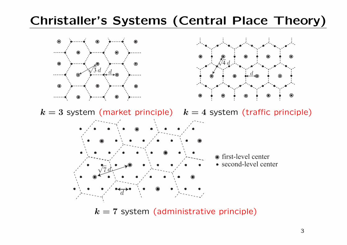
Christaller’s Systems (Central Place Theory)
3
4
k = 3 system (market principle) k = 4 system (traffic principle)
first-level center
second-level center
k = 7 system (administrative principle)
3

Benard Convection in Fluid Dynamics
Hexagonal tessellation
Successful math analysis by
group-theoreticbifurcation theory
(群論的分岐理論)
Koschmieder (1974) Benard convection, Adv in Chemical Physics
4

Bifurcation Theory for (分岐理論)Hexagonal Agglomeration in (人口集積)Economic Geography (経済地理学)
Part 1: (background)
Economic Geography
Part 2: (result)
Hexagonal Agglomeration
Part 3: (methodology)
Group-Theoretic Bifurcation Theory
5

Part 1.
Economic Geography
6

Economic Geography (経済地理学)
von Thunen (1826): von Thunen Ring
Christaller (1933), Losch (1940):Central Place Theory (中心地理論)
New Economic Geography (新経済地理学)
Krugman (1991):Increasing returns and economic geography
Fujita, Krugman, Venables (1999):The Spatial Economy:Cities, Regions, and International Trade(空間経済学:都市・地域・国際貿易の新しい分析)
Fujita (2010): The evolution of spatial economics:
from Thunen to the New Economic Geography
7

Southern GermanyChristaller 1933
Munich
Nuremberg
Frankfurt
Stuttgart
8

Christaller’s Systems (Central Place Theory)
Christaller’s k = 3 system Christaller’s k = 4 system
Christaller’s k = 7 system
9

Losch’s Hexagons
d/ 2d/ 2
d/ 2
d/ 2d/ 2d/ 2
d/ 2d/ 2
d/ 2
d/ 2
10

Economic Geography / Central Place Theory
- descriptive / normative approach
- no mechanism (micro-economic, mathematical)
New Econ. Geography / Spatial Economics
- micro-economic mechanism
core-periphery model: transport cost,market equilibrium, population migration
Our Study
- mathematical mechanism
pattern formation, bifurcation
-
6economic
modeling
spatialplatform
11

Core–Periphery Model
An economy with n places: i = 1, . . . , n
Two industrial sectors:
- agriculture: perfectly competitive, · · ·- manufacturing: imperfectly competitive,
transport cost, increasing returns, · · ·Two types of labour:
- farmers: immobile
- workers: mobile
.......................
.......................
12

Core-Periphery Model
• Market equilibrium (short-run)
Given: λi: population in place i (= 1, 2, . . . , n)
τ : transport cost parameter
• Population migration (long-run)dλi
dt= Fi(λ, τ ) i = 1, . . . , n
e.g.: Replicator dynamics (Krugman, 1991)
Fi(λ, τ ) = (ωi(λ, τ )− ω(λ, τ ))λi, i = 1, . . . , n
− Market equil. =⇒ real wage ωi = ωi(λ, τ )
− Average real wage ω =n∑
i=1
λiωi
13

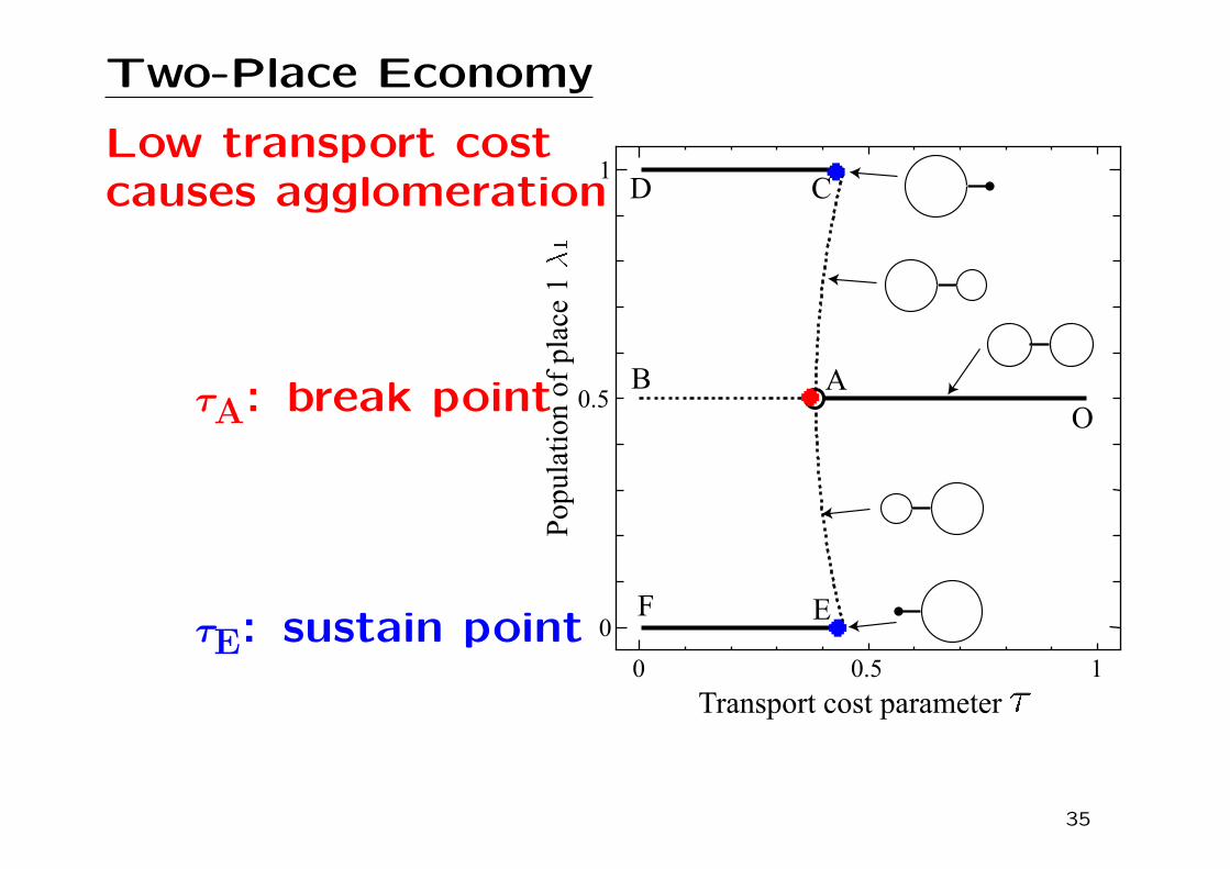
Two-Place Economy
λ1 + λ2 = 1, λ1, λ2 ≥ 0
transport cost:T = 1/(1− τ )
(a) λ1 = λ2 (b) λ1 = λ2
Y1 = µλ1w1 +1− µ
2, Y2 = µλ2w2 +
1− µ
2
G1 = [λ1w11−σ + λ2(w2T )1−σ]
11−σ
G2 = [λ1(w1T )1−σ + λ2w21−σ]
11−σ
w1 = [Y1G1σ−1 + Y2G2
σ−1T 1−σ]1σ
w2 = [Y1G1σ−1T 1−σ + Y2G2
σ−1]1σ
ω1 = w1G1−µ, ω2 = w2G2
−µ
dλ1
dt= (ω1(λ, τ )− ω2(λ, τ ))λ1λ2
14

Two-Place Economy
Low transport costcauses agglomeration
0 0.5 1
0
0.5
1
O
AB
CD
EF
Transport cost parameter
Popula
tion o
f pla
ce 1
τA: break point ●
τE: sustain point ●
●
15

New Econ. Geography: State-of-the-Art
- Micro-economic model:
core-periphery → refinements
- Spatial platform:
two-place → long narrow, racetrack
Krugman (1996): The Self-organizing EconomyI have demonstrated the emergence of a regular lattice only for
a one-dimensional economy, but I have no doubt that a better
mathematician could show that a system of hexagonal market
areas will emerge in two dimensions.
16

Long Narrow Economy
Fujita, Mori (1997): Regional Sci Urban Econ
Structural stability and evolution of urban systems
Fujita, Krugman, Mori (1999): Euro Econ Review
On the evolution of hierarchical urban systems
Racetrack EconomyKrugman (1993): Euro Econ Review
On the number and location of cities
Mossay (2003): Regional Sci Urban Econ
Increasing returns and heterogeneity in a spatial economy
Picard, Tabuchi (2010): Economic Theory
Self-organized agglomerations and transport costs
Tabuchi, Thisse (2011): J. Urban EconomicsA new economic geography model of central places
17

Part 2.
Hexagonal Agglomeration
18
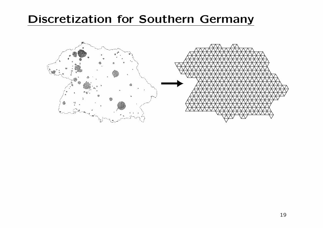
Discretization for Southern Germany
19

Initial Stages (high transport cost)
= 14.00 −→ = 12.74 −→ = 11.97
(D=3)√L/d= 3
A B C (l/d =√3)
= 11.16 −→ = 10.23 −→ = 9.57
L/d=2(D=12)
√ 3
D E F (l/d = 2√3)
20

Final Stages (low transport cost)
= 2.73 −→ = 2.57 −→ = 2.30
G H I
= 2.00 −→ = 1.60 −→ = 0.03
J K L
21

Numerical Analysis for Southern Germanypopulation vs transport cost
0.2
0.4
0.6
0.8
0 2 4 6 8 10 12 14
I
1.0
BCDFG
E
H
J
K
L
Transport cost parameter
i
A
14
C
12 13
0.01
0
A
B
BA
F E
0.03
0
(a)
(b)
9.5 10 10.5
(c)
2.3 2.5 2.70
0.5
G
H
0
K
(Forslid–Ottaviano model (2003), logit choice function)
22

Modeling by Periodic Finite Hexagonal Lattice
2
15 16
1
2 x
y
1
1 2
15 16
1 2
15 16
1 2
15 16
1 2
15 16
(a) 4× 4 lattice (b) Periodically repeated
23

Emergence of Central Places (1)market principle k = 3
multiplicity M = 2
9× 9 lattice
0 1 2 3 4
0
0.2
0.4
0.6
0.8
1
Transport cost parameter
max
M = 2
M = 6
M = 12
ABCD E
FG
H
AE
I
F
k = 3 (D = 3)
D = 1
D = 81
D = 9 D = 27
O
1/81
(Forslid–Ottaviano model (2003), logit choice function)
24

Emergence of Central Places (2)
traffic principle k = 4
multiplicity M = 3
16× 16 lattice
0 2 4 610
−3
10−2
10−1
1
OAB
CD
M=6
M=3 E
FGH
IJ
max
D 1
D 4
D 16
D 64
Transport cost parameter
25

Emergence of Central Places (3)
1
ACO
D
F
2 3
max
0
0.2
0.1
B
E
M = 6
M = 12
Transport cost parameter
k = 7 (D =7)
1/49
administrativeprinciple k = 7
multiplicityM = 12
7× 7 lattice
26

Summary of Our Results
Christaller’s size n Mult Mk = 3 (market) 3 × 2k = 4 (traffic) 2 × 3k = 7 (administrative) 7 × 12
Losch’s D size n Mult M9 (traffic-like) 3 × 612 (market-like) 6 × 613 (admin-like) 13 × 1216 (traffic-like) 4 × 619 (admin-like) 19 × 1221 (admin-like) 21 × 1225 (traffic-like) 5 × 6
27

Lattice Economy• Ikeda, Murota, Akamatsu, Kono, Takayama,Sobhaninejad, Shibasaki (2010):
Self-organizing hexagons in economic agglomeration: core-periphery
models and central place theory, METR 2010-28, U. Tokyo.
Discovery of hexagonal patterns (numerical, theoretical)
• Takayama, Akamatsu (2010): 土木計画学研究・論文集.
• Ikeda, Murota, Akamatsu (2012): Self-organization of
Losch’s hexagons in economic · · · , Int. J. Bifurcation & Chaos.
• Ikeda, Murota, Akamatsu, Kono, Takayama (2014):Self-organization of hexagonal · · · , J. Economic Behav. & Organiz.
• Ikeda, Murota (2014):Bifurcation Theory for Hexagonal Agglomeration inEconomic Geography.Systematic presentation of the theory
28
Part 3.
Group-Theoretic
Bifurcation Theory
29
Group-theoretic Bifurcation Theory
• Sattinger (1979):Group Theoretic Methods in Bifurcation Theory.
(Lecture Notes in Mathematics)
• Golubitsky, Schaeffer (1985):Singularities and Groups in Bifurcation Theory, Vol. 1
• Golubitsky, Stewart, Schaeffer (1988):Singularities and Groups in Bifurcation Theory, Vol. 2
30

Bifurcation Analysis of Two-Place Economy
poplutation λ = (λ1, λ2), transport cost τ
F (λ, τ ) =
[F1(λ1, λ2, τ )F2(λ1, λ2, τ )
]= 0
F1(λ1, λ2, τ ) = (ω1(λ1, λ2, τ )− ω(λ1, λ2, τ ))λ1
F2(λ1, λ2, τ ) = (ω2(λ1, λ2, τ )− ω(λ1, λ2, τ ))λ2
average real wage ω(λ1, λ2, τ ) = λ1ω1 + λ2ω2
Symmetry: F2(λ1, λ2, τ ) = F1(λ2, λ1, τ )
31

Formulation of Symmetry
Symmetry: F2(λ1, λ2, τ ) = F1(λ2, λ1, τ )
⇐⇒ [0 11 0
] [F1(λ, τ )F2(λ, τ )
]= F
( [0 11 0
]λ, τ
)⇐⇒Equivariance: T (g)F (λ, τ ) = F (T (g)λ, τ ), g ∈ G
G = {e, s}: group, s : (1, 2) 7→ (2, 1),
T (e) =
[1 00 1
], T (s) =
[0 11 0
]
32

Reduction to Bifurcation Equation
Critical point (λc, τc) = (1/2, 1/2, τc) at some τ = τc
New variable w = λ1 − λ2; f = τ − τc
λ1 =1 + w
2, λ2 =
1− w
2
⇓ Bifurcation equation:
F (w, f) = F1
(1 + w
2,1− w
2, f
)− F2
(1 + w
2,1− w
2, f
)= w[A f + Bw2 + · · · ] = 0
⇓ Two kinds of solutions (equilibria):{w = 0, trivial equilibria (λ1 = λ2),
f = −BAw2 + · · · bifurcating equilibria (λ1 = λ2)
33

Pitchfork Bifurcation
subcritical supercritical
(A < 0, B > 0) (A < 0, B < 0)
◦: bifurcation point, —: stable, −−−: unstable
� �
34
Two-Place Economy
Low transport costcauses agglomeration
0 0.5 1
0
0.5
1
O
AB
CD
EF
Transport cost parameter
Popula
tion o
f pla
ce 1
τA: break point ●
τE: sustain point ●
●
35

Methodological Characteristics
Group-theoretic method shows:
(1) Reduction to bifurcation equationdimension (# vars/eqns), choice of vars
(2) Possible bifurcating equilibriasymmetry/pattern (e.g., Christaller’s systems)
(3) Generic (structural) properties under symmetry,independent of individual models and parametersstructural degeneracy vs accidental coincidence
Does not capture:
(1) Specific value of τc
(2) Specific values of A, B, etc.
(3) Stability of equilibria-
6
economicmodeling
(spatial)symmetry
36

Equivariance for Hexagonal Lattice
T (g)F (λ, τ ) = F (T (g)λ, τ ), g ∈ G
G = · · ·
T (g) = · · ·
37

Symmetry of 3 x 3 Lattice G = ⟨r, s, p1, p2⟩
21 3
4 5 6
7 8 9
21 3
4 5 6
7 8 9
rotation r reflection s
21 3
4 5 6
7 8 9
21 3
4 5 6
7 8 9
translation p1 translation p2
38

Representation Matrices T (n = 3)
r 7→
11
11
11
11
1
, s 7→
11
11
11
11
1
p1 7→
11
11
11
11
1
, p2 7→
11
11
11
11
1
G = ⟨r, s, p1, p2⟩
39

Equivariance for Hexagonal Lattice
T (g)F (λ, τ ) = F (T (g)λ, τ ), g ∈ G
G = ⟨r, s, p1, p2⟩
T (g) =
1
11
11
11
11
(etc.)
40

Symmetry of n× n Lattice
2
15 16
1
2 x
y
1
r: rotation (π/3 rad)
s: reflection
p1, p2: translations
G = ⟨r, s, p1, p2⟩= D6 ⋉ (Zn × Zn)
r6 = s2 = (rs)2 = p1n = p2
n = e, p2p1 = p1p2,
rp1 = p1p2r, rp2 = p−11 r, sp1 = p1s, sp2 = p−11 p−12 s
41

Subgroups for Christaller’s Systems
Symmetry: G = ⟨r, s, p1, p2⟩ = D6 ⋉ (Zn × Zn)
Partial Symmetry:
⟨r, s, p21p2, p−11 p2⟩ ⟨r, s, p21, p
22⟩ ⟨r, p31p2, p
−11 p22⟩
k = 3 k = 4 k = 7
42

Reduction to Bifurcation Equation
Liapunov-Schmidt reductioneliminates variables by implicit function thm
Which variables remain?
Jc: Jacobian at critical point
dim Ker(Jc) = dim of bifur.eqn (# eqns/vars)
Ker(Jc): invariant subspace ←→ irred representation(generically)
dim bifur.eqn = dim irred rep in T
= 2, 3, 6, 12 [NOT: 4]
Bifurcation eqn: F (λ, τ ) = 0
Equivariance: T (g)F (λ, τ ) = F (T (g)λ, τ ), g ∈ G
43

Group Representation
Representation of G is a mapping T : G→ GL(N,R):
T (gh) = T (g)T (h), g, h ∈ G.
Invariant subspace: w ∈W ⇒ T (g)w ∈W (∀g ∈ G)
Irreducible rep: does not have invariant subspaces
A finite family determined by G
Decomposition into irred reps: (essent.) unique for T
Q−1TQ = T (1) ⊕ T (2) ⊕ T (3) ⊕ · · ·
44

Irreducible Decomposition (n = 3)
Q−1T (g)Q = Q−1
11
11
11
11
1
Q
=
∗∗ ∗∗ ∗
∗ ∗ ∗ ∗ ∗ ∗∗ ∗ ∗ ∗ ∗ ∗∗ ∗ ∗ ∗ ∗ ∗∗ ∗ ∗ ∗ ∗ ∗∗ ∗ ∗ ∗ ∗ ∗∗ ∗ ∗ ∗ ∗ ∗
dim: 1 + 2 + 6
45

Procedure of Group-th. Bifurcation Analysis
• Find symmetry group G & representation T
• Enumerate all irred reps µ of G
1,2,3,4,6,12-dim (by method of little groups)
• Decompose T into irred reps µ
• For each irred rep µ:
A: Derive and solve bifurcation eqnto find bifur. solution and see the symmetry
B: Apply equivariant branching lemmato see the existence of specified symmetry
46

Irreducible Representations of G = ⟨r, s, p1, p2⟩
n dim1 dim2 dim3 dim4 dim 6 dim 12
6m 4 4 4 1 2n− 6 (n2 − 6n + 12)/12
6m± 1 4 2 0 0 2n− 2 (n2 − 6n + 5)/12
6m± 2 4 2 4 0 2n− 4 (n2 − 6n + 8)/12
6m± 3 4 4 0 1 2n− 4 (n2 − 6n + 9)/12
• dim 6 exist for n ≥ 3 • dim 12 exist for n ≥ 6
n dim1 dim2 dim3 dim4 dim 6 dim 123 4 4 0 1 2 06 4 4 4 1 6 17 4 2 0 0 2 1
47

3-dim Irreducible Rep
r : (w1, w2, w3) 7→ (w3, w1, w2)s : (w1, w2, w3) 7→ (w3, w2, w1)
p1 : (w1, w2, w3) 7→ (−w1, w2,−w3)p2 : (w1, w2, w3) 7→ (w1,−w2,−w3)
T (r) =
11
1
T (s) =
11
1
T (p1) =
−1 1−1
T (p2) =
1−1−1
(3;+,+)
48

Bifurcation Equations for M = 3 (1)
Fi(w1, w2, w3, τ ) = 0 (i = 1, 2, 3)
Equivariance conditions:
r : F3(w1, w2, w3) = F1(w3, w1, w2)
F1(w1, w2, w3) = F2(w3, w1, w2)
F2(w1, w2, w3) = F3(w3, w1, w2)
s : F3(w1, w2, w3) = F1(w3, w2, w1)
F2(w1, w2, w3) = F2(w3, w2, w1)
F1(w1, w2, w3) = F3(w3, w2, w1)
p1 : −F1(w1, w2, w3) = F1(−w1, w2,−w3)
F2(w1, w2, w3) = F2(−w1, w2,−w3)
−F3(w1, w2, w3) = F3(−w1, w2,−w3)
p2 : F1(w1, w2, w3) = F1(w1,−w2,−w3)
−F2(w1, w2, w3) = F2(w1,−w2,−w3)
−F3(w1, w2, w3) = F3(w1,−w2,−w3)
49

Bifurcation Equations for M = 3 (2)
Conditions connecting F2 to (F1, F3):
F1(w1, w2, w3) = F2(w3, w1, w2)
F3(w1, w2, w3) = F2(w2, w3, w1)
Conditions on F2:
F2(w1, w2, w3) = F2(−w1, w2,−w3)
−F2(w1, w2, w3) = F2(w1,−w2,−w3)
F2(w1, w2, w3) = F2(w3, w2, w1)
⇓F2 = w2
∑a=0
∑b=0
∑c=0
A2a,2b+1,2c(τ )w12aw2
2bw32c
+ w1w3
∑a=0
∑b=0
∑c=0
A2a+1,2b,2c+1(τ )w12aw2
2bw32c
50

Bifurcation Equations for M = 3 (3)
F2 = w2
∑∑∑A2a,2b+1,2c(τ )w1
2aw22bw3
2c
+ w1w3
∑∑∑A2a+1,2b,2c+1(τ )w1
2aw22bw3
2c
F1 = F2(w3, w1, w2), F3 = F2(w2, w3, w1)
Trivial solution: w1 = w2 = w3 = 0
Bifurcating solution: w1 = w2 = w3 = 0
0 =∑∑∑
A2a,2b+1,2c(τ )w12(a+b+c)
+ w1
∑∑∑A2a+1,2b,2c+1(τ )w1
2(a+b+c)
≈ Aτ + Bw1
−→ w1 ≈ −(A/B)τ
51

Bifurcation Equations for M = 3 (4)
Symmetry of (w,w,w) = ⟨r, s, p21, p22⟩
⟨r, s, p21p2, p−11 p2⟩ ⟨r, s, p21, p
22⟩ ⟨r, p31p2, p
−11 p22⟩
k = 3 k = 4 k = 7
52

Bifurcation Equations for M = 3 (5)
F2 = w2
∑∑∑A2a,2b+1,2c(τ )w1
2aw22bw3
2c
+ w1w3
∑∑∑A2a+1,2b,2c+1(τ )w1
2aw22bw3
2c
F1 = F2(w3, w1, w2), F3 = F2(w2, w3, w1)
Another bifurcating solution: w2 = 0, w1 = w3 = 0
0 =∑
A0,2b+1,0(τ )w22b ≈ Aτ + Bw2
2
−→ τ ≈ −(B/A)Bw22
⟨r3, s, p1, p22⟩53

12-dim Irreducible Rep(12; k, ℓ) (1 ≤ ℓ ≤ k − 1, 2k + ℓ ≤ n− 1)
r 7→
S
SS
SS
S
, s 7→
I
II
II
I
p1 7→ p2 7→
Rk
Rℓ
R−k−ℓ
Rk
Rℓ
R−k−ℓ
,
Rℓ
R−k−ℓ
Rk
R−k−ℓ
Rk
Rℓ
R =
[cos(2π/n) − sin(2π/n)sin(2π/n) cos(2π/n)
], S =
[1−1
], I =
[1
1
]54

12-dim Irreducible Rep (complex variables)
(12; k, ℓ) (1 ≤ ℓ ≤ k − 1, 2k + ℓ ≤ n− 1)
r :
z1z2z3z4z5z6
7→z3z1z2z5z6z4
s :
z1z2z3z4z5z6
7→z4z5z6z1z2z3
p1 :
z1z2z3z4z5z6
7→
ωk z1ωℓ z2
ω−k−ℓ z3ωk z4ωℓ z5
ω−k−ℓ z6
p2 :
z1z2z3z4z5z6
7→
ωℓ z1ω−k−ℓ z2ωk z3
ω−k−ℓ z4ωk z5ωℓ z6
ω = exp(i2π/n)
55
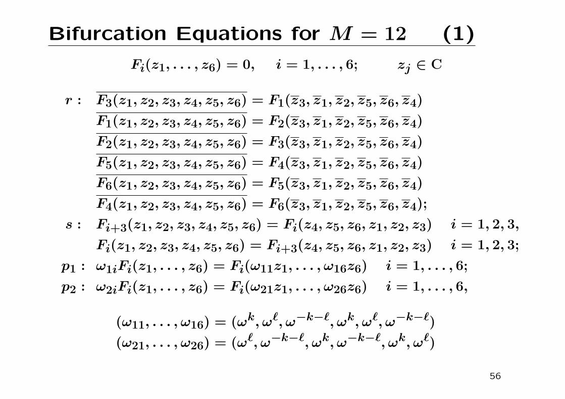
Bifurcation Equations for M = 12 (1)
Fi(z1, . . . , z6) = 0, i = 1, . . . , 6; zj ∈ C
r : F3(z1, z2, z3, z4, z5, z6) = F1(z3, z1, z2, z5, z6, z4)
F1(z1, z2, z3, z4, z5, z6) = F2(z3, z1, z2, z5, z6, z4)
F2(z1, z2, z3, z4, z5, z6) = F3(z3, z1, z2, z5, z6, z4)
F5(z1, z2, z3, z4, z5, z6) = F4(z3, z1, z2, z5, z6, z4)
F6(z1, z2, z3, z4, z5, z6) = F5(z3, z1, z2, z5, z6, z4)
F4(z1, z2, z3, z4, z5, z6) = F6(z3, z1, z2, z5, z6, z4);
s : Fi+3(z1, z2, z3, z4, z5, z6) = Fi(z4, z5, z6, z1, z2, z3) i = 1, 2, 3,
Fi(z1, z2, z3, z4, z5, z6) = Fi+3(z4, z5, z6, z1, z2, z3) i = 1, 2, 3;
p1 : ω1iFi(z1, . . . , z6) = Fi(ω11z1, . . . , ω16z6) i = 1, . . . , 6;
p2 : ω2iFi(z1, . . . , z6) = Fi(ω21z1, . . . , ω26z6) i = 1, . . . , 6,
(ω11, . . . , ω16) = (ωk, ωℓ, ω−k−ℓ, ωk, ωℓ, ω−k−ℓ)
(ω21, . . . , ω26) = (ωℓ, ω−k−ℓ, ωk, ω−k−ℓ, ωk, ωℓ)
56

Bifurcation Equations for M = 12 (2)
Conditions connecting F1 to (F2, . . . , F6):
F2(z1, z2, z3, z4, z5, z6) = F1(z2, z3, z1, z6, z4, z5)
F3(z1, z2, z3, z4, z5, z6) = F1(z3, z1, z2, z5, z6, z4)
F4(z1, z2, z3, z4, z5, z6) = F1(z4, z5, z6, z1, z2, z3)
F5(z1, z2, z3, z4, z5, z6) = F1(z5, z6, z4, z3, z1, z2)
F6(z1, z2, z3, z4, z5, z6) = F1(z6, z4, z5, z2, z3, z1)
Conditions on F1:
F1(z1, z2, . . . , z6) = F1(z1, z2, . . . , z6)
ω11F1(z1, z2, . . . , z6) = F1(ω11z1, ω12z2, . . . , ω16z6)
ω21F1(z1, z2, . . . , z6) = F1(ω21z1, ω22z2, . . . , ω26z6)
(ω11, . . . , ω16) = (ωk, ωℓ, ω−k−ℓ, ωk, ωℓ, ω−k−ℓ)(ω21, . . . , ω26) = (ωℓ, ω−k−ℓ, ωk, ω−k−ℓ, ωk, ωℓ)
57

Bifurcation Equations for M = 12 (3)k = 7
⟨r, p31p2, p−11 p22⟩ = symmetry of (x, x, x, 0, 0, 0)
Targeted solution: (z1, z2, z3, z4, z5, z6) = (x, x, x, 0, 0, 0)
Bifur. eqn: Fi(z1, z2, z3, z4, z5, z6) = 0 (i = 1, . . . , 6)
⇐⇒ F1(x, x, x, 0, 0, 0) = 0, F1(0, 0, 0, x, x, x) = 0
58

Bifurcation Equations for M = 12 (4)For (k, ℓ, n) = (2, 1, 7):
F1 = A1z1 + (A2z2z3 + A3z1z3 + A4z22)
+ (A5z21z1 + A6z1z2z2 + A7z1z3z3 + A8z1z4z4
+ A9z1z5z5 + A10z1z6z6 + A11z1z2z3 + A12z2z23
+ A13z22z3 + A14z
21z2 + A15z
33) + · · ·
⇓F1(x, x, x, 0, 0, 0) = A1x + (A2 + A3 + A4)x
2
+ (A5 + A6 + · · ·+ A15)x3 + · · ·
≈ x(Aτ + Bx)
F1(0, 0, 0, x, x, x) = 0=⇒ x ≈ −(A/B)τ
59

Bifurcation Equations for M = 12 (5)For (k, ℓ, n) = (2, 1, 6):
F1 = A1z1 + A2z2z3 + (A3z21z1 + A4z1z2z2 + A5z1z3z3
+ A6z1z4z4 + A7z1z5z5 + A8z1z6z6 + A9z2z4z6
+ A10z3z4z5 + A11z1z2z6 + A12z23z4 + A13z1z
25)
+ [A14z4z26 + A15z5z
36 + A16z5z
36 + · · · ] + · · ·
⇓F1(x, x, x, 0, 0, 0) = A1x + A2x
2 + (A3 + A4 + A5)x3 + · · ·
F1(0, 0, 0, x, x, x) = A14x3 + (A15 + A16)x
4 + · · ·
Two equations in one variable x
=⇒ No solution exists
60

Bifurcation at 12-fold Critical Point
Irred rep: (12; k, ℓ)
gcd(k − ℓ, n) ∈ 3Z gcd(k − ℓ, n) ∈ 3ZD ∈ 3Z D ∈ 3Z
GCD-div traffic-like market-like
(type V) (type M)
GCD-div traffic-like (V) market-like (M)
admin-like (T) admin-like (T)
k =k
gcd(k, ℓ, n), ℓ =
ℓ
gcd(k, ℓ, n), n =
n
gcd(k, ℓ, n)
GCD-div:(k − ℓ) gcd(k, ℓ) is divisible by gcd(k2 + kℓ + ℓ2, n)
61

Summary of Our Results (again)
Christaller’s size n Mult Mk = 3 (market) 3 × 2k = 4 (traffic) 2 × 3k = 7 (administrative) 7 × 12
Losch’s D size n Mult M9 (traffic-like) 3 × 612 (market-like) 6 × 613 (admin-like) 13 × 1216 (traffic-like) 4 × 619 (admin-like) 19 × 1221 (admin-like) 21 × 1225 (traffic-like) 5 × 6
62

Group Appendix
(i) Associative law: (g h) k = g (h k)
(ii) ∃ identity element e: e g = g e = g (∀g ∈ G)
(iii) ∀g ∈ G, ∃h (inverse of g): g h = h g = e
Dihedral group D6
D6 = ⟨r, s⟩ = {e, r, r2, . . . , r5, s, sr, sr2, . . . , sr5}
r6 = s2 = (sr)2 = e
Semidirect product G = D6⋉(Zn × Zn)• Zn × Zn is a normal subgroup of G
• unique representation g = ha (h ∈ D6, a ∈ Zn × Zn)
63

Equivariant Branching Lemma Appendix
Assume that rep T is absolutely irreducible and the
bifurcation equation is “generic.”
For an isotropy subgroup Σ with dim Fix(Σ) = 1,
there exists a unique smooth solution branch s.t.
Σ(w) = Σ for each solution w on the branch.
Σ(w) = {g ∈ G | T (g)w = w}
Fix(Σ) = {w | T (g)w = w for all g ∈ Σ}
64