kurs komputerowy s - mathematica - cz. 3 -...
TRANSCRIPT

OBLICZENIA NUMERYCZNE, Karolina Mikulska-Ruminska
Kurs komputerowy S - Mathematica
- cz. 3
Suma i iloczyn elementow ciagu
NSum[wyr, {zm, w_pocz, w_konc}], NProduct[wyr, {zm, w_pocz,
w_konc}]
? *Sum*
System‘
DivisorSum NSumTerms RootSum SumConvergence
NSum ParallelSum Sum
UniformSumDistributio-
n
NSum@1 � x^3, 8x, 1, 20<D
1.20087
NSum@1 � x^2, 8x, 1, Infinity<D
1.64493
Sum@1 � x^2, 8x, 1, Infinity<D
Π2
6
Pi^2 � 6.0
1.64493
Options@NSumD
8AccuracyGoal ® ¥, Compiled ® Automatic, EvaluationMonitor ® None,
Method ® Automatic, NSumTerms ® 15, PrecisionGoal ® Automatic,
VerifyConvergence ® True, WorkingPrecision ® MachinePrecision<
NSum@1 � x^2, 8x, 1, Infinity<, WorkingPrecision ® 30D
1.644934066848226436472

NSum@1 � x^2, 8x, 1, 5<, WorkingPrecision ® 20,
EvaluationMonitor :> Print@"x = ", x, "\t", N@1 � x^2, 5DDD
x = 1.0000000000000000000 1.0000
x = 2.0000000000000000000 0.25000
x = 3.0000000000000000000 0.11111
x = 4.0000000000000000000 0.062500
x = 5.0000000000000000000 0.040000
1.4636111111111111111
NProduct@x^2 � Hx + 10L, 8x, 1, 10<D
19.641
Product@x^2 � Hx + 10L, 8x, 1, 10<D
907 200
46 189
N@%D H* otrzymamy numeryczna postac wyrazenia *L
19.641
Rozwiazywanie rownan
NSolve[rown, zm]
rown = 2 x^2 + 8 x - 2 � 0
-2 + 8 x + 2 x2
� 0
NSolve@rown, xD
88x ® -4.23607<, 8x ® 0.236068<<
Solve@rown, xD
99x ® -2 - 5 =, 9x ® -2 + 5 ==
Clear@a, b, cD
2 KursS_cz3.nb

NSolve@a x^2 + b x + c � 0, xD
::x ®
0.5 -1. b - 1. b2 - 4. a c
a
>, :x ®
0.5 -1. b + b2 - 4. a c
a
>>
FindRoot[wielomian, zm]
w = x^4 - 4 x^3 - 5 x^2 + 5 x + 3
FindRoot@w, 8x, 1<D
3 + 5 x - 5 x2
- 4 x3
+ x4
8x ® 1.<
FindRoot@w, 8x, -1<D
8x ® -1.32632<
Plot@w, 8x, -2, 2<D
-2 -1 1 2
-20
-10
10
20
KursS_cz3.nb 3

Interpolacja, ekstrapolacja, aproksymacja
Interpolation[dane], gdzie dane = {k1,k2,k3} lub dane={{x1,y1},
{x2,y2}, {x3,y3}, .. , {xn, yn}} lub dane = {{{x1,k1, ...}, y1},
{{x2,k2,..},y2}, ...}
Interpolation[dane, wart]
f = Interpolation@81, 3, 5, 8, 5, 2, 5, 7, 5<D
InterpolatingFunction@881, 9<<, <>D
3.9375
Plot@f@xD, 8x, 1, 9<D
4 6 8
2
3
4
5
6
7
8
4 KursS_cz3.nb

Show@%, ListPlot@81, 3, 5, 8, 5, 2, 5, 7, 5<DD
4 6 8
2
3
4
5
6
7
8
k = 881, 1<, 82, 4<, 85, 3<, 86, 8<, 84, 3<, 87, 4<<
881, 1<, 82, 4<, 85, 3<, 86, 8<, 84, 3<, 87, 4<<
f1 = Interpolation@kD
InterpolatingFunction@881, 7<<, <>D
Show@Plot@f1@xD, 8x, 1, 7<D, ListPlot@kDD
2 3 4 5 6 7
2
3
4
5
6
7
8
Options@InterpolationD
8InterpolationOrder ® 3, Method ® Automatic, PeriodicInterpolation ® False<
o = 81, 3, 5, 8, 5, 2, 5, 7, 5<
81, 3, 5, 8, 5, 2, 5, 7, 5<
KursS_cz3.nb 5
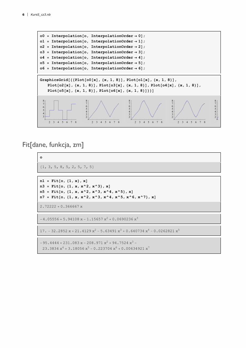
o0 = Interpolation@o, InterpolationOrder ® 0D;
o1 = Interpolation@o, InterpolationOrder ® 1D;
o2 = Interpolation@o, InterpolationOrder ® 2D;
o3 = Interpolation@o, InterpolationOrder ® 3D;
o4 = Interpolation@o, InterpolationOrder ® 4D;
o5 = Interpolation@o, InterpolationOrder ® 5D;
o6 = Interpolation@o, InterpolationOrder ® 6D;
GraphicsGrid@88Plot@o0@xD, 8x, 1, 8<D, Plot@o1@xD, 8x, 1, 8<D,
Plot@o2@xD, 8x, 1, 8<D, Plot@o3@xD, 8x, 1, 8<D, Plot@o4@xD, 8x, 1, 8<D,
Plot@o5@xD, 8x, 1, 8<D, Plot@o6@xD, 8x, 1, 8<D<<D
2 3 4 5 6 7 8
3
4
5
6
7
8
2 3 4 5 6 7 8
2
3
4
5
6
7
8
2 3 4 5 6 7 8
2
3
4
5
6
7
8
2 3 4 5 6 7 8
2
3
4
5
6
7
8
2
3
4
5
6
7
8
Fit[dane, funkcja, zm]
o
81, 3, 5, 8, 5, 2, 5, 7, 5<
n1 = Fit@o, 81, x<, xDn3 = Fit@o, 81, x, x^2, x^3<, xDn5 = Fit@o, 81, x, x^2, x^3, x^4, x^5<, xDn7 = Fit@o, 81, x, x^2, x^3, x^4, x^5, x^6, x^7<, xD
2.72222 + 0.366667 x
-4.05556 + 5.94108 x - 1.15657 x2
+ 0.0690236 x3
17. - 32.2852 x + 21.4129 x2
- 5.63491 x3
+ 0.640734 x4
- 0.0262821 x5
-95.4444 + 231.083 x - 208.971 x2
+ 94.7524 x3
-
23.3834 x4
+ 3.18056 x5
- 0.223704 x6
+ 0.00634921 x7
6 KursS_cz3.nb

GraphicsGrid@88Show@Plot@n1, 8x, 0, 9<, PlotRange -> 880, 9<, 8-5, 15<<D, ListPlot@oDD,
Show@Plot@n3, 8x, 0, 9<, PlotRange -> 880, 9<, 8-5, 15<<D, ListPlot@oDD<,
8Show@Plot@n5, 8x, 0, 9<, PlotRange -> 880, 9<, 8-5, 15<<D, ListPlot@oDD,
Show@Plot@n7, 8x, 0, 9<, PlotRange -> 880, 9<, 8-5, 15<<D, ListPlot@oDD<<D
2 4 6 8
-5
0
5
10
15
2 4 6 8
-5
0
5
10
15
2 4 6 8
-5
0
5
10
15
2 4 6 8
-5
0
5
10
15
FindFit[dane, funkcja, param, zm]
FindFit[dane, {funkcja, warunki}, param, zm]
d@x1_, x2_, x3_D := x1 H1 - E^H-x2 Hx - x3LLL^2
dd = d@1, 0.5, 2D
I1 - ã-0.5 H-2+xLM2
KursS_cz3.nb 7

Plot@dd, 8x, 0, 10<D
2 4 6 8 10
0.5
1.0
1.5
2.0
wartosci = Table@8x, dd<, 8x, 0, 10<D
880, 2.95249<, 81, 0.420839<, 82, 0.<,
83, 0.154818<, 84, 0.399576<, 85, 0.603527<, 86, 0.747645<,
87, 0.842568<, 88, 0.902905<, 89, 0.940517<, 810, 0.963704<<
fdd = Fit@wartosci, 81, x, x^2, x^3, x^4, x^5<, xDShow@Plot@fdd, 8x, 0, 10<D, ListPlot@wartosciDD
2.92535 - 3.81667 x + 1.70151 x2
- 0.324345 x3
+ 0.0284033 x4
- 0.000936548 x5
2 4 6 8 10
0.5
1.0
1.5
2.0
2.5
8 KursS_cz3.nb

Clear@a, b, cDffdd = FindFit@wartosci, a H1 - E^H-b Hx - cLLL^2, 8a, b, c<, xDShow@Plot@d@a, b, cD �. ffdd, 8x, 0, 10<D, ListPlot@wartosciDD
8a ® 1., b ® 0.5, c ® 2.<
2 4 6 8 10
0.5
1.0
1.5
2.0
Maksimum i minimum funkcji
FindMinimum[funkcja, {zm, wartosc}], NMinimize[funkcja, zm],
FindMaximum[funkcja, {zm, wartosc}], NMaximize[funkcja, zm].
g = x^4 - 5 x^3 - x^2 + 2 x - 1
Plot@g, 8x, -2, 5.5<D
-1 + 2 x - x2
- 5 x3
+ x4
-2 -1 1 2 3 4 5
-60
-40
-20
20
40
60
FindMinimum@g, 8x, 0<D
8-1.61526, 8x ® -0.411847<<
KursS_cz3.nb 9

FindMinimum@g, 8x, 1<D
8-73.7496, 8x ® 3.8462<<
NMinimize@g, xD
8-73.7496, 8x ® 3.8462<<
FindMaximum@g, 8x, -1<D
FindMaximum::cvmit : Failed to converge to the requested accuracy or precision within 100 iterations. �
95.770242244403928 ´ 10417
, 9x ® -2.75612 ´ 10104==
NMaximize@g, xD
NMaximize::cvdiv : Failed to converge to a solution. The function may be unbounded. �
92.902057384546909 ´ 10422
, 9x ® -4.1274 ´ 10105==
i = 1;
FindMinimum@g, 8x, 1<,
EvaluationMonitor :> HPrint@"i=", i, " ", "x=", xD; i++LD
i=1 x=1.
i=2 x=1.5
i=3 x=3.5
i=4 x=12.1245
i=5 x=4.28748
i=6 x=3.82898
i=7 x=4.12001
i=8 x=3.84547
i=9 x=3.84621
i=10 x=3.8462
8-73.7496, 8x ® 3.8462<<
Calkowanie i rownania rozniczkowe
W wyniku obliczen symbolicznych jako rozwiazanie otrzymujemy
funkcje w postaci symbolicznej, a wyniku obliczen numerycznych
otrzymujemy przyblizone warto�ci funkcji dla pewnych wybranych
punktow z jej dziedziny.
/http://pl.wikipedia.org/wiki/Obliczenia_symboliczne/
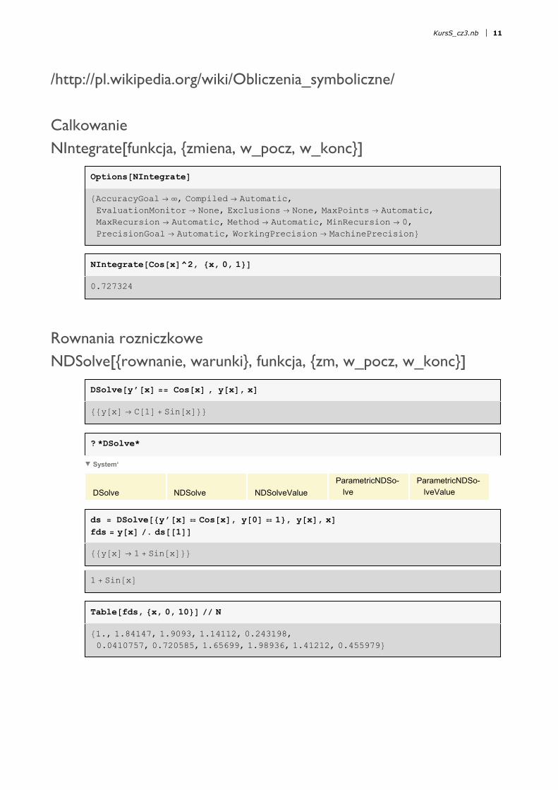
Calkowanie
NIntegrate[funkcja, {zmiena, w_pocz, w_konc}]
10 KursS_cz3.nb
Calkowanie i rownania rozniczkowe
W wyniku obliczen symbolicznych jako rozwiazanie otrzymujemy
funkcje w postaci symbolicznej, a wyniku obliczen numerycznych
otrzymujemy przyblizone warto�ci funkcji dla pewnych wybranych
punktow z jej dziedziny.
/http://pl.wikipedia.org/wiki/Obliczenia_symboliczne/
Calkowanie
NIntegrate[funkcja, {zmiena, w_pocz, w_konc}]
Options@NIntegrateD
8AccuracyGoal ® ¥, Compiled ® Automatic,
EvaluationMonitor ® None, Exclusions ® None, MaxPoints ® Automatic,
MaxRecursion ® Automatic, Method ® Automatic, MinRecursion ® 0,
PrecisionGoal ® Automatic, WorkingPrecision ® MachinePrecision<
NIntegrate@Cos@xD^2, 8x, 0, 1<D
0.727324
Rownania rozniczkowe
NDSolve[{rownanie, warunki}, funkcja, {zm, w_pocz, w_konc}]
DSolve@y’@xD == Cos@xD , y@xD, xD
88y@xD ® C@1D + Sin@xD<<
? *DSolve*
System‘
DSolve NDSolve NDSolveValue
ParametricNDSo-
lve
ParametricNDSo-
lveValue
ds = DSolve@8y’@xD � Cos@xD, y@0D � 1<, y@xD, xDfds = y@xD �. ds@@1DD
88y@xD ® 1 + Sin@xD<<
1 + Sin@xD
Table@fds, 8x, 0, 10<D �� N
81., 1.84147, 1.9093, 1.14112, 0.243198,
0.0410757, 0.720585, 1.65699, 1.98936, 1.41212, 0.455979<
KursS_cz3.nb 11
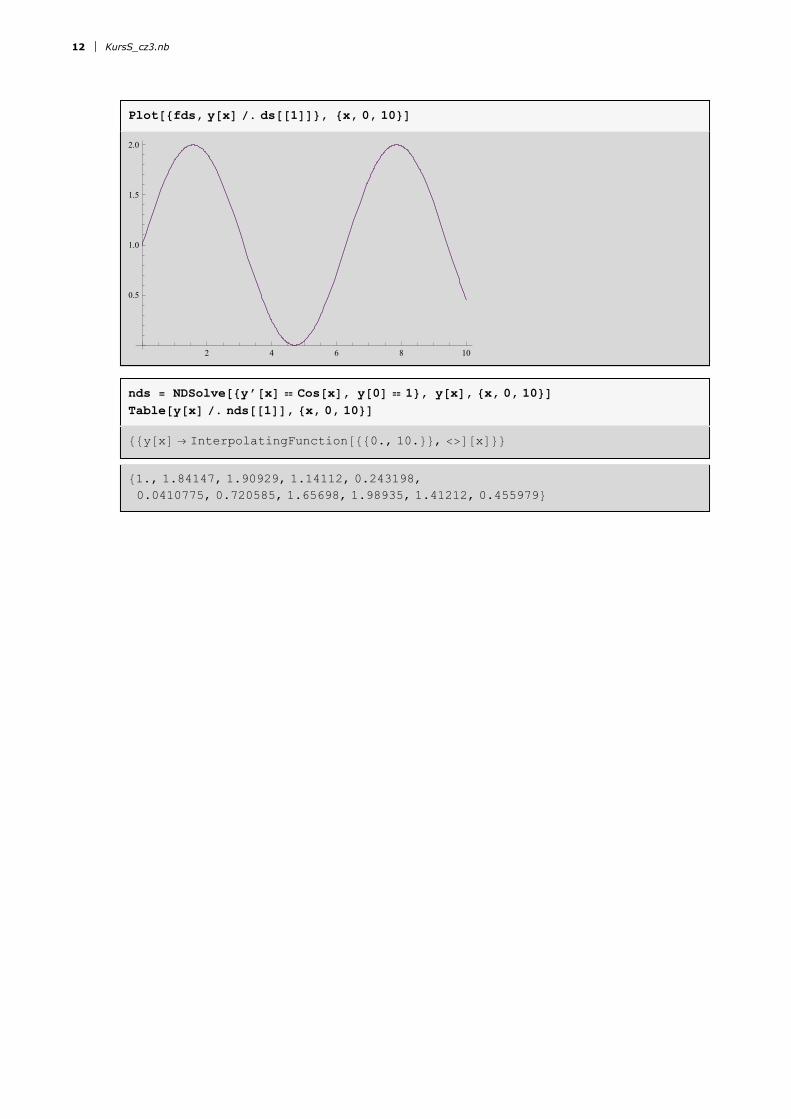
Plot@8fds, y@xD �. ds@@1DD<, 8x, 0, 10<D
2 4 6 8 10
0.5
1.0
1.5
2.0
nds = NDSolve@8y’@xD � Cos@xD, y@0D � 1<, y@xD, 8x, 0, 10<DTable@y@xD �. nds@@1DD, 8x, 0, 10<D
88y@xD ® InterpolatingFunction@880., 10.<<, <>D@xD<<
81., 1.84147, 1.90929, 1.14112, 0.243198,
0.0410775, 0.720585, 1.65698, 1.98935, 1.41212, 0.455979<
12 KursS_cz3.nb