kronecker products image restoration - emory university
TRANSCRIPT

Kronecker Productsin
Image Restoration
James G. Nagy
Emory University
Atlanta, GA
Julie Kamm (Raytheon)
Lisa Perrone (Emory)
Michael Ng (HKU)
Misha Kilmer (Tufts)

Kronecker Product
C ⊗D =
c11D c12D · · · c1nDc21D c22D · · · c2nD
... ... ...cm1D cm2D · · · cmnD
Properties: • (C ⊗D)T = CT ⊗DT
• (C ⊗D)−1 = C−1 ⊗D−1
• (CDE)⊗(FGH) = (C⊗F )(D⊗G)(E⊗H)
• (C ⊗D)x ⇔ DXCT , x = vec(X)

Image Restoration
Given distorted image, reconstruct picture of original scene
b = Ax + n
b = distorted (blurred and noisy) image
x = true image
n = noise
A = matrix modeling distortion process
Computational Problem:
Given b, A, find an approximation of x

Regularization
• Problem: Given b = Ax + n, compute x
• Ill-conditioned A ⇒ x̂ = A−1b is bad!
• Regularization ⇒ math trick to stabilize numerical scheme.
– Regularization by filtering
e.g., using singular value decomposition (SVD)

Regularization
• Problem: Given b = Ax + e, compute x
• Ill-conditioned A ⇒ x̂ = A−1b is bad!
• Regularization ⇒ math trick to stabilize numerical scheme.
– Regularization by filtering
e.g., using singular value decomposition (SVD)
– Regularization by iteration
e.g., using conjugate gradients (CG)

Outline
1. Regularization by filtering.
2. Constructing the matrix A.
(Kronecker products)
3. Regularization by iteration.
4. Summary.

Regularization by Filtering
Suppose A = UΣV T , UTU = I, V TV = I
Σ =diagonal matrix
Then the ”inverse” solution is
x = A−1b
= V Σ−1UTb
=n∑
i=1
uTi b
σivi
Regularization by Filtering
Suppose A = UΣV T , UTU = I, V TV = I
Σ =diagonal matrix
Then the ”inverse” solution is
x̂ = A−1(b + ε)
= V Σ−1UT (b + ε)
=n∑
i=1
uTi (b + ε)
σivi

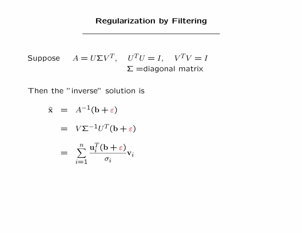
Regularization by Filtering
Suppose A = UΣV T , UTU = I, V TV = I
Σ =diagonal matrix
Then the ”inverse” solution is
x̂ = A−1(b + ε)
= V Σ−1UT (b + ε)
=n∑
i=1
uTi (b + ε)
σivi
=n∑
i=1
uTi b
σivi +
n∑i=1
uTi ε
σivi
= x + error

Regularization by Filtering
Basic Idea: Filter out problems caused by small singular values.
That is, compute:
xreg =N∑
i=1
φiuT
i b
σivi
where the “filter factors” satisfy:
φi ≈{
1 if σi is large0 if σi is small

Regularization by Filtering
• Truncated SVD (of pseudo inverse filter)
xtsvd =k∑
i=1
uTi b
σivi
• Tikhonov
xtik =N∑
i=1
σ2i
σ2i + α2
uTi b
σivi

Regularization by Filtering
One method to choose regularization parameters is:
Generalized Cross Validation
For example, in Tikhonov, choose α to minimize
GCV (α) =
NN∑
i=1
(uT
i b
σ2i + α2
)2
N∑i=1
1
σ2i + α2
2

Regularization by Filtering
How to efficiently compute SVD of large matrix?
Exploit structure of A:
1. Circulant ⇒ use Fourier transform:
A = F∗ΛF
2. ”Symmetric” Toeplitz + Hankel ⇒ use cosine transform:
A = CTΛC
3. Kronecker product ⇒ use SVD:
A = C ⊗D = (UcΣcVTc )⊗ (UdΣdV
Td )
= (Uc ⊗ Ud)(Σc ⊗Σd)(Vc ⊗ Vd)T

Constructing matrix A
• Assume distortion operation is ”spatially invariant”
• Choose an appropriate boundary condition
( e.g., zero, periodic, reflexive)
• Build matrix one column at a time:
i-th column = Aei ,
where ei = i-th unit vector

Constructing matrix A
Build matrix one column at a time, using imaging system:
• Suppose ei = ith unit vector
point source

Constructing matrix A
Build matrix one column at a time, using imaging system:
• Suppose ei = ith unit vector
• Then Aei = ith column of A
point source point spread function (PSF)

Constructing matrix A
Spatially invariant ⇒ distortion independent of position

Constructing matrix A
Spatially invariant ⇒ distortion independent of position

Constructing matrix A
Spatially invariant ⇒ distortion independent of position
Each column of A is identical, modulo shift
⇒ one PSF is enough to describe A
⇒ A has Toeplitz structure

Constructing matrix A: Example 1
e5 =
000010000
→
0 0 00 1 00 0 0
→ blur →
p11 p12 p13
p21 p22 p23
p31 p32 p33
→ Ae5 =
p11
p12
p13
p21
p22
p23
p31
p32
p33
A =
p11
p12
p13
p21
p22
p23
p31
p32
p33

Constructing matrix A: Example 1
e5 =
000010000
→
0 0 00 1 00 0 0
→ blur →
p11 p12 p13
p21 p22 p23
p31 p32 p33
→ Ae5 =
p11
p12
p13
p21
p22
p23
p31
p32
p33
A =
p12 p11
p13 p12 p11
p13 p12
p22 p21
p23 p22 p21
p23 p22
p32 p31
p33 p32 p31
p33 p32

Constructing matrix A: Example 1
e5 =
000010000
→
0 0 00 1 00 0 0
→ blur →
p11 p12 p13
p21 p22 p23
p31 p32 p33
→ Ae5 =
p11
p12
p13
p21
p22
p23
p31
p32
p33
A =
p22 p21 p12 p11
p23 p22 p21 p13 p12 p11
p23 p22 p13 p12
p32 p31 p22 p21 p12 p11
p33 p32 p31 p23 p22 p21 p13 p12 p11
p33 p32 p23 p22 p13 p12
p32 p31 p22 p21
p33 p32 p31 p23 p22 p21
p33 p32 p23 p22
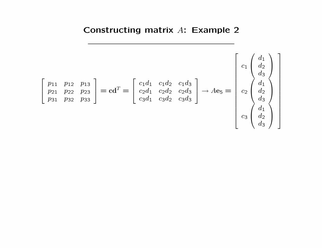
Constructing matrix A: Example 2
p11 p12 p13
p21 p22 p23
p31 p32 p33
= cdT =
c1d1 c1d2 c1d3
c2d1 c2d2 c2d3
c3d1 c3d2 c3d3
→ Ae5 =
c1
d1
d2
d3
c2
d1
d2
d3
c3
d1
d2
d3

Constructing matrix A: Example 2
p11 p12 p13
p21 p22 p23
p31 p32 p33
= cdT =
c1d1 c1d2 c1d3
c2d1 c2d2 c2d3
c3d1 c3d2 c3d3
→ Ae5 =
c1
d1
d2
d3
c2
d1
d2
d3
c3
d1
d2
d3
c1
d1
d2
d3
c2
d1
d2
d3
c3
d1
d2
d3

Constructing matrix A: Example 2
p11 p12 p13
p21 p22 p23
p31 p32 p33
= cdT =
c1d1 c1d2 c1d3
c2d1 c2d2 c2d3
c3d1 c3d2 c3d3
→ Ae5 =
c1
d1
d2
d3
c2
d1
d2
d3
c3
d1
d2
d3
c1
d2 d1
d3 d2 d1
d3 d2
c2
d2 d1
d3 d2 d1
d3 d2
c3
d2 d1
d3 d2 d1
d3 d2

Constructing matrix A: Example 2
p11 p12 p13
p21 p22 p23
p31 p32 p33
= cdT =
c1d1 c1d2 c1d3
c2d1 c2d2 c2d3
c3d1 c3d2 c3d3
→ Ae5 =
c1
d1
d2
d3
c2
d1
d2
d3
c3
d1
d2
d3
c2
d2 d1
d3 d2 d1
d3 d2
c1
d2 d1
d3 d2 d1
d3 d2
c3
d2 d1
d3 d2 d1
d3 d2
c2
d2 d1
d3 d2 d1
d3 d2
c1
d2 d1
d3 d2 d1
d3 d2
c3
d2 d1
d3 d2 d1
d3 d2
c2
d2 d1
d3 d2 d1
d3 d2
= C ⊗D

Kronecker Product Summary
If point spread function satisfies: P = cdT , then
• Zero BC ⇒ A = C ⊗D, where C and D are Toeplitz
• Periodic BC ⇒ A = C ⊗D, where C and D are circulant
• Reflexive BC⇒ A = C⊗D, where C and D are Toeplitz+Hankel

General Kronecker Product Decomposition
• If point spread function satisfies: P =r∑
k=1
ckdTk , then
A =r∑
k=1
Ck ⊗Dk
• Optimal approximation using work by Pitsianis and Van Loan
(Kamm, N., 2000; N., Ng, Perrone, 2003)
• For 3-dimensional problems, need tensor decompositions.

Kronecker Product Approximations
Optimal approximations (2-D problems):
• P =r∑
k=1
σkukvTk ⇒ σ1u1v
T1 = best rank-1 approximation
• Setting c1 =√
σ1u1 and d1 =√
σ1v1, then
A ≈ C1 ⊗D1 = best Kronecker product approximation

Kronecker Product Approximations
Optimal approximations (2-D problems):
• P =r∑
k=1
σkukvTk ⇒ σ1u1v
T1 = best rank-1 approximation
• Setting c1 =√
σ1u1 and d1 =√
σ1v1, then
A ≈ C1 ⊗D1 = best Kronecker product approximation
= (UcΣcVTc )⊗ (UdΣdV
Td ) = SVD approximation

Kronecker Product Approximations
Optimal approximations (2-D problems):
• P =m∑
k=1
σkukvTk ⇒
m∑k=1
σkukvTk = rank-m approximation
• Setting ck =√
σkuk and dk =√
σkvk, then
A ≈m∑
k=1
Ck ⊗Dk = sum of Kronecker product approximation

Kronecker Product Approximations
Optimal approximations (2-D problems):
A =r∑
k=1
Ck ⊗Dk ≈ (Uc ⊗ Ud)Σ(Vc ⊗ Vd)T
where C1 = UcΣcVTc , D1 = UdΣdV
Td
minΣ
||A− (Uc ⊗ Ud)Σ(Vc ⊗ Vd)T ||F
Σ = diag((Uc ⊗ Ud)
TA(Vc ⊗ Vd))
= diag
(Uc ⊗ Ud)T
r∑k=1
Ck ⊗Dk
(Vc ⊗ Vd)

Kronecker Product Approximations
For 3-D problems:
• Need orthogonal tensor decompositions
SIMAX: de Lathauwer, de Moor, Vandewalle, ’00;
Kolda, ’01;
Zhang, Golub, ’01
• We use HOSVD (de Lathauwer, de Moor, Vandewalle, ’00):
P =r1∑
i=1
r2∑j=1
r3∑k=1
σijkui ◦ vj ◦wk .
• These vectors define matrices Ci, Dj and Fk, with
A =∑ ∑
σijk 6=0
∑Ci ⊗Dj ⊗ Fk ,

SVD Summary
The PSF and boundary condition define A:
• Periodic BC ⇒ FFT decomposition O(n2 logn)
• Reflexive BC, symmetric PSF⇒ DCT decomposition O(n2 logn)
• Otherwise Kronecker product approximation⇒ SVD O(n3)

SVD Summary
The PSF and boundary condition define A:
• Periodic BC ⇒ FFT decomposition O(n2 logn)
• Reflexive BC, symmetric PSF⇒ DCT decomposition O(n2 logn)
• Otherwise Kronecker product approximation⇒ SVD O(n3)
In MATLAB:
>> A = psfMatrix(PSF, ’boundary condition’);
>> [U, S, V] = svd(A);
>> x = TSVD(U, S, V, b);

Iterative Regularization
We consider algorithms (e.g., conjugate gradients) of the form
x0 = initial estimate of xfor j = 0,1,2, . . .
• xj+1 = computations involving xj, A,preconditioner matrix, M
• determine if stopping criteria are satisfiedend
Need to efficiently:
multiply with A, AT
solve linear systems with M , MT .

Multiply with A
• Use FFTs to form convolutions on padded arrays
• Padding depends on:
– boundary condition
– support (size) of PSF
• Can also do spatially variant blurs.

Preconditioning
Typical approach for Ax = b
Find matrix M satisfying the following properties:
• Inexpensive to “construct” M .
• Inexpensive to solve Mz = w.
• M−1A ≈ I (singular values of M−1A cluster around 1).

Preconditioning
“Ideal” preconditioner: M = A = UΣV T
• Solving Mz = w ⇒ z = V Σ−1UTw.
• For ill-posed problems, noise/errors in w are amplified.

Preconditioning
“Ideal” preconditioner: M = A = UΣV T
• Solving Mz = w ⇒ z = V Σ−1UTw.
• For ill-posed problems, noise/errors in w are amplified.
• Remedy: Regularize using truncated SVD
z = V Σ†UTw
where Σ† =diag(1/σ1, . . . ,1/σk,0, . . . ,0)
• Problem: The matrix M is singular.

Preconditioning Ill-Posed Problems
Modify TSVD idea (Hanke, N., Plemmons, ’93)
z = V Σ−1τ UTw
where
• Σ−1τ =diag(1/σ1, . . . ,1/σk,1, . . . ,1)
• σk ≥ τ > σk
That is, the preconditioner is:
Mτ = UΣτV T

Preconditioning Ill-Posed Problems
Notice that the preconditioned system is:
M−1τ A = (UΣτV T )−1(UΣV T )
= V Σ−1τ ΣV T
= V ∆V T
where ∆ =diag(1, . . . ,1, σk+1, . . . , σn)
That is,
• Large (good) singular values clustered at 1.
• Small (bad) singular values not clustered.

Preconditioning Summary
• Construct preconditioner by approximating A with either
FFT, DCT or SVD
• Use modified TSVD to regularize preconditioner.
In MATLAB:
>> A = psfMatrix(PSF, ’boundary condition’);
>> M = svdPrec(A, b);
The End!
• Exploiting Kronecker product structure in image restoration
– Can be effective in filtering methods that use SVD
– Can be effective as preconditioners
• Matlab software:
http://www.mathcs.emory.edu/∼nagy/RestoreTools/
• Related software for ill-posed problems (Hansen, Jacobsen)
http://www.imm.dtu.dk/∼pch/Regutools/