Kronecker Product Matrices for Compressive Sensing

Marco F. Duarte and Richard G. Baraniuk∗

Technical Report TREE-1105Department of Electrical and Computer Engineering

Rice University

March 17, 2011

Abstract

Compressive sensing (CS) is an emerging approach for the acquisition of signals havinga sparse or compressible representation in some basis. While the CS literature has mostlyfocused on problems involving 1-D signals and 2-D images, many important applications involvemultidimensional signals; in this case, CS works best with representations that encapsulate thestructure of such signals in every dimension. We propose the use of Kronecker product matricesin CS for two purposes. First, such matrices can act as sparsifying bases that jointly modelthe different types of structure present in the signal. Second, the measurement matrices usedin distributed settings can be easily expressed as Kronecker product matrices. The Kroneckerproduct formulation in these two settings enables the derivation of analytical bounds for sparseapproximation of multidimensional signals and CS recovery performance as well as a means toevaluate novel distributed measurement schemes.

1 Introduction

1.1 CS and multidimensional signals

Compressive sensing (CS) is a new approach to simultaneous sensing and compression that enablesa potentially large reduction in the sampling and computation costs at a sensor for a signal xhaving a sparse or compressible representation θ in some basis Ψ (i.e. x = Ψθ) [1, 2]. By a sparserepresentation, we mean that only K out of the N signal coefficients in θ are nonzero, with K N .By a compressible representation, we mean that the coefficient’s magnitudes, when sorted, have afast power-law decay, i.e.,

|θ(i)| < Ci−1/p (1)

∗MFD is with the Department of Computer Science, Duke University, Durham, NC 27708. RGB is with the Depart-ment of Electrical and Computer Engineering, Rice University, Houston, TX 77005. Email: marco.duarte@duke.edu,richb@rice.edu. Web: dsp.rice.edu. This work was completed while MFD was a Ph.D. student at Rice University, andwas supported by grants NSF CCF-0431150 and CCF-0728867, DARPA/ONR N66001-08-1-2065, ONR N00014-07-1-0936 and N00014-08-1-1112, AFOSR FA9550-07-1-0301, ARO MURIs W911NF-07-1-0185 and W911NF-09-1-0383,and the Texas Instruments Leadership Program.

for p ≤ 1 and C <∞. Many natural signals are sparse or compressible; for example, smooth signalsare compressible in the Fourier basis, while piecewise smooth signals and images are compressiblein a wavelet basis.

CS builds on the work of Candes, Romberg, and Tao [1] and Donoho [2], who showed that asignal having a sparse or compressible representation in one basis can be recovered from its linearprojections onto a small set of M = O (K log(N/K)) measurement vectors that are incoherent withthe sparsifying basis, meaning that the representation of the measurement vectors in this basis isnot sparse. When the measurement vectors are stacked as rows of a measurement matrix Φ, theCS measurements can be expressed as a vector

y = Φx (2)

of length M . CS acquisition devices multiplex the signal, as they read inner products of the signalvector against the measurement vectors instead of reading the signal vector itself [3]. We can obtaina compressed representation of the signal by obtaining a number of inner products smaller than thesignal length. Random vectors play a central role as universal measurements in the sense that theyare incoherent with any fixed basis with high probability. The CS measurement process is nonadap-tive, and the recovery process is nonlinear; there exist a variety of CS recovery algorithms inspiredby sparse approximation techniques [1, 2, 4, 5]. To recover the signal from the measurements, wesearch for the sparsest signal among all those that yield the observed measurement values.

The CS literature has mostly focused on problems involving single sensors and one-dimensional(1-D) signal or 2-D image data. However, some important applications that hold the most promisefor CS involve higher-dimensional signals. The coordinates of these signals may span several physi-cal, temporal, or spectral dimensions. Additionally, these signals are often captured in a progressivefashion, in a sequence of captures corresponding to subsets of the coordinates. Examples includehyperspectral imaging (with spatial and spectral dimensions), video acquisition (with spatial andtemporal dimensions), and synthetic aperture radar imaging (with progressive acquisition in thespatial dimensions). Another class of promising applications for CS involves distributed networksor arrays of sensors, including for example environmental sensors, microphone arrays, and cameraarrays.

These properties of multidimensional data and the corresponding acquisition hardware compli-cate the design of both the measurement matrix Φ and the sparsifying basis Ψ to achieve maximumefficiency in CS.

1.2 CS measurement matrices for multidimensional signals

For signals of any dimension, global CS measurements that multiplex most or all of the values ofthe signal together (corresponding to dense matrices Φ) are required for universality, since theyare needed to capture arbitrary sparsity structure [6]. However, for multidimensional signals, suchmeasurements require the use of multiplexing sensors that operate simultaneously along all datadimensions, increasing the physical complexity or acquisition time/latency of the CS device. Inmany settings it can be difficult to implement such multiplex sensors due to the large dimensionalityof the signals involved and the ephemeral availability of the data during acquisition. For example,each image frame in a video sequence is available only for a limited time; therefore, any multiplexingsensor that calculates global CS measurements would have to sum of the M partial inner productsfrom each of the frames from the beginning to the end of the video sequence. Similarly, global CS

2

measurements of a hyperspectral datacube would require simultaneous multiplexing in the spectraland spatial dimensions, which is a challenge with current optical and spectral modulators [7, 8];such separate multiplexing nature limits the structure of the measurements obtained.

These application-specific limitations naturally point us in the direction of measurement systemsΦ that depend only on a portion of the entries of the multidimensional signal being acquired. Manyapplications and practical hardware designs demand partitioned measurements that process only aportion of the multidimensional signal at a time. Each portion usually corresponds to a section ofthe signal along a given dimension, such as one frame in a video signal or the image of one spectralband of a hyperspectral datacube.

1.3 Sparsifying bases for multidimensional signals

For multidimensional signals, we can often characterize the signal structure present on each of itsdifferent dimensions or coordinates in terms of a sparse representation. For example, each imageframe in a video sequence is often sparse or compressible in a wavelet basis, since it correspondsto an image obtained at a particular time instant. Simultaneously, the temporal structure of eachpixel in a video sequence is often smooth or piecewise smooth, due to camera movement, objectmotion and occlusion, illumination changes, etc. A similar situation is observed in hyperspectralsignals: the reflectivity values at a given spectral band correspond to an image with known structure;additionally, the spectral signature of a given pixel is usually smooth or piecewise smooth, dependingon the spectral range and materials present in the observed area.

Initial work on the sparsity and compressibility of multidimensional signals and signal ensemblesfor CS [9–21] has provided new sparsity models for multidimensional signals. These models considersections of the multidimensional data corresponding to fixed values for a subset of the coordinatesas separate signals and pose correlation models between the values and locations of their sparserepresentations. To date, the resulting models are rather limited in the types of structures admitted.For almost all models, theoretical guarantees on signal recovery have been provided only for strictlysparse signals, for noiseless measurement settings, or in asymptotic regimes. Additionally, almostall of these models are tied to ad-hoc signal recovery procedures.

Clearly, more generic models for sparse and compressible multidimensional signals are needed inorder to leverage the CS framework to a higher degree of effective compression. Ideally, we shouldbe able to formulate a sparsifying basis for the entire multidimensional signal that simultaneouslyaccounts for all the types of structure present in the data.

In this paper, we show that Kronecker product matrices offer a natural means to generate bothsparsifying bases Ψ and measurement matrices Φ for CS of multidimensional signals, resulting ina formulation that we dub Kronecker Compressive Sensing (KCS). Kronecker product sparsifyingbases combine the structures encoded by the sparsifying bases for each signal dimension into a singlematrix. Kronecker product measurement matrices can be implemented by performing a sequenceof separate multiplexing operations on each signal dimension. The Kronecker product formulationfor sparsifying bases and measurement matrices enables the derivation of analytical bounds forrecovery of compressible multidimensional signals from randomized or incoherent measurements.

1.4 Stylized applications

To better motivate the KCS concept, we consider now in more detail three relevant multidimensionalCS applications: hyperspectral imaging, video acquisition, and distributed sensing.

3

(a) (b) (c)

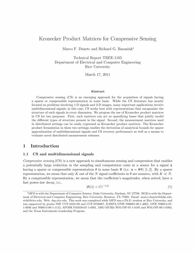
Figure 1: Example capture from a single-pixel hyperspectral camera [22] at resolution N = 128 × 128 pixels × 64spectral bands (220 voxels) for the 450nm–850nm wavelength range from M = 4096 CS measurements per band (4×sub-Nyquist) [23]. (a) Mandrill test image printed and illuminated by a desk lamp for acquisition. (b) Hyperspectraldatacube obtained via independent CS recovery of each spectral band as a separate image. (c) Hyperspectral datacubeobtained via KCS; marked improvement is seen in bands with low signal-to-noise ratios. Data courtesy of Kevin Kelly,Ting Sun, and Dharmpal Takhar from Rice University.

1.4.1 Hyperspectral imaging

Consider the single-pixel hyperspectral camera (SPHC) [7, 22], where the hyperspectral lightfieldis focused onto a digital micromirror device (DMD). The DMD acts as a optical spatial modula-tor and reflects part of the incident lightfield into a scalar spectrometer. In this way, the DMDcomputes inner products of the image of each spectral band in the hyperspectral lightfield againsta measurement vector with 0/1 entries, coded in the orientation of the mirrors. Each spectralband’s image is multiplexed by the same binary functions, since the DMD reflects all of the imagedspectra simultaneously. This results in the same measurement matrix Φ being applied to eachspectral band image. The resulting measurement matrix applied to the hyperspectral datacubecan be represented as a Kronecker product IS ⊗ Φ, where IS is an S × S identity matrix and Sdenotes the number of spectral bands recorded. Additionally, there are known sparsifying bases foreach spectral band image as well as each pixel’s spectral signature, which can be integrated into asingle Kronecker product sparsifying basis. An example datacube captured with a SPHC via KCSis shown in Fig. 1 [23].

1.4.2 Video acquisition

Consider the example of compressive video acquisition, where a single-pixel camera applies the sameset of measurements to each image frame in the video sequence, resulting once again in a Kroneckerproduct measurement matrix [10]. We can sparsify or compress the temporal structure at eachpixel using a Fourier or wavelet transform depending on the video characteristics. Furthermore,we can sparsify each image frame using a standard cosine or wavelet transform. We can then usea Kronecker product of these two bases to sparsify or compress the video sequence.

4

1.4.3 Distributed sensing

In distributed sensing problems, we aim to acquire an ensemble of signals x1, . . . ,xJ ∈ RN thatvary in time, space, etc. We assume that each signal’s structure can be encoded using sparsitywith an appropriate basis Ψ1. This ensemble of signals can be expressed as a N × J matrix

X = [x1 x2 . . . xJ ] = [x1T x2T . . . xNT

]T , where the individual signals x1, . . . ,xj correspondingto columns of the matrix, and where the rows x1, . . . ,xN of the matrix correspond to differentsnapshots of the signal ensemble at different values of time, space, etc. Under this construction,the structure of each signal is observable on each of the columns of the matrix, while the structureof each snapshot (spanning all the signals) is present on each of the rows of the matrix X.

We expect that, in certain applications, the snapshot structure can also be modeled using spar-sity; that is, that a basis or frame Ψ2 can be used to compress or sparsify x1, . . . xN . For example,in sensor network applications, the structure of each snapshot is determined by the geometry ofthe sensing deployment, and can also be captured by a sparsity basis [24]. In such cases, we obtaina single sparsifying basis Ψ1 ⊗ Ψ2 for the signal ensemble x that encodes the structure of boththe signals and the snapshots; such representation significantly simplifies the analysis of the signalensemble sparsity and compressibility. Furthermore, if separate measurements yj = Φxj of eachsignal are obtained using the same measurement Φ, we can express the resulting measurementmatrix acting on the signal ensemble as the Kronecker product IJ ⊗ Φ.

1.5 Contributions

This paper has three main contributions. First, we propose Kronecker product matrices as sparsi-fying bases for multidimensional signals to jointly model the signal structure along each one of itsdimensions. In some cases, such as Kronecker product wavelet bases, we can to obtain bounds forthe magnitude rate of decay of the signal coefficients for certain kinds of data. This rate of decayis dependent on the rates of decay for the coefficients of sections of the signals across the differentdimensions using the individual bases. When the rates of decay using the corresponding bases foreach of the dimensions are different, we show that the Kronecker product basis rate falls betweenthe maximum and minimum rates among the different dimensions; when the rates of decay are allthe same, they are matched by that of the Kronecker product basis.

Second, we show that several different CS measurements schemes proposed for multidimensionalsignals can be easily expressed in our Kronecker product framework. In particular, when partitionedmeasurements are used and the same measurement matrix is applied to each portion of the signal,the resulting measurement matrix can be expressed as the Kronecker product of an identity matrixwith the measurement matrix. We can also build new D-stage CS acquisition devices that useKronecker measurement matrices: the first stage applies the same lower-dimensional measurementmatrix on each portion of the signal along its first dimension, and each subsequent stage appliesadditional low-dimensional measurement matrices on previously obtained measurements along theremaining dimensions of the signal. The resulting measurement matrix for the high-dimensionalsignal is simply the Kronecker product of the low-dimensional matrices used at each stage.

Third, we provide metrics to evaluate partitioned measurement schemes against Kroneckermeasurement matrices, as well as guidance on the improvements that may be afforded by the useof such multidimensional structures. In particular, we provide some initial results by studyingthe special case of signals that are compressible in a Kronecker product of wavelet bases. We alsocompare the rate of decay for the recovery error of KCS to the rate of decay for the recovery error of

5

standard CS recovery from separate measurements of each portion of the signal. Finally, we verifyour theoretical findings using experimental results with synthetic and real-world multidimensionalsignals.

This paper is organized as follows. Section 2 provides background in compressive sensing andtensor and Kronecker products. Section 3 introduces Kronecker compressive sensing, and Section 4provides initial results for wavelet-sparse signals. Section 5 provides experimental results, Section 6summarizes related work, and Section 7 closes the document with conclusions and suggestions forfuture work.

2 Background

2.1 Compressive sensing

Compressive sensing (CS) is a efficient signal acquisition framework for signals that are sparse orcompressible in an appropriate domain. Let x ∈ RN be the signal of interest. We say that anorthonormal basis1 Ψ ∈ RN×N sparsifies the signal x if θ = ΨTx has only K nonzero entries, withK N and ΨT denoting the transpose of Ψ. We then say that x is K-sparse or has sparsity Kin Ψ. Similarly, we say that Ψ compresses x if the entries of θ, when sorted by magnitude, decayaccording to (1). In this case, we say that θ is in weak `p (noted as θ ∈ w`p) or, alternatively,that θ is s-compressible in Ψ, with s = 1/p− 1/2. Such vectors can be compressed using transformcoding by preserving only the coefficients with largest absolute magnitude; we term by θK theapproximation with the K largest coefficients of θ. Thus, for a K-sparse signal, the approximationerror σK(θ) := ‖θ − θK‖2 = 0, where ‖ · ‖2 denotes the `2 or Euclidean norm. For s-compressiblesignals, σK(θ) ≤ C ′K−s, i.e., the approximation error decays exponentially. Many types of signalsof interest are known to be compressible in appropriate bases. For example, smooth signals suchas audio recordings are compressible in the Fourier basis, and piecewise smooth signals such asnatural images are compressible in a wavelet basis.

The CS acquisition procedure consists of measuring inner products of the signal against a set ofmeasurement vectors φ1, . . . , φM; when M < N , the acquisition procedure effectively compressesthe signal. By collecting the measurement vectors as rows of a measurement matrix Φ ∈ RM×N ,the acquisition procedure can be written as y = Φx = ΦΨθ, with the vector y ∈ RM containingthe CS measurements.

The goal of CS is to recover the full signal x from the fewest possible measurements y. Infinitelymany vectors x can yield the recorded measurements y due to the rank deficiency of the matrixΥ = ΦΨ. One of the main enablers of CS was the discovery that when the signal being observed issparse enough, it can be exactly recovered by solving the linear program [1, 2, 25]

θ = arg min ‖θ‖1 s.t. y = Υθ. (3)

In this case, ‖ · ‖1 denotes the `1 norm, which is equal to the sum of the absolute values of thevector entries.

In the real world, the CS measurements are corrupted by noise. This provides us with CSmeasurements y = Φx + n, with n denoting the noise vector. In this case, the signal can also be

1In the sequel, we will use the same notation Ψ to refer to the set of basis vectors and to the matrix having thesebasis vectors as columns.

6

successfully recovered using the quadratic program [1]

θ = arg min ‖θ‖1 s.t. ‖y −Υθ‖2 ≤ ε, (4)

where ε is an upper bound on the `2 norm of the noise vector n. The penalty paid is an additionaldistortion in the recovered version of the signal proportional to ε in the worst case.

Previous contributions have posed conditions on the number and type of measurement vectorsnecessary for signal recovery [1, 26]. The Restricted Isometry Property (RIP) has been proposedto measure the fitness of a matrix Υ for CS.

Definition 2.1 The K-restricted isometry constant for the matrix Υ, denoted by δK , is the small-est nonnegative number such that, for all θ ∈ RN with ‖θ‖0 = K,

(1− δK)‖θ‖22 ≤ ‖Υθ‖22 ≤ (1 + δK)‖θ‖22.

Once the RIP constants are determined, they can be used to provide guarantees for CS recovery.

Theorem 2.1 [27] If the matrix Υ has δ2K <√

2− 1, then the solution θ to (4) obeys

‖θ − θ‖2 ≤ C0‖θ − θK‖1K1/2

+ C1ε,

where C0 and C1 are fixed constants dependent on δ2K .

In words, Theorem 2.1 guarantees that sparse signals can be recovered perfectly from noiselessmeasurements; that compressible signals can be recovered to a distortion similar to that of thetransform coding compression; and that the recovery process is robust to the presence of noisein the measurements. Unfortunately, calculating the RIP constants for a given matrix requirescombinatorially complex computation. Interestingly, many probabilistic classes of matrices havebeen advocated. For example, a matrix of size M ×N with independent and identically distributednormal entries with variance 1/M obeys the condition of Theorem 2.1 with very high probability ifK ≤ O (M/ log(N/M)) [1, 2, 6]. The same is true of matrices following Rademacher or subgaussiandistributions.

In some applications, the sensing system constrains the types of measurement matrices that arefeasible. This could be due either to the computational power needed to generate the matrix, ordue to limitations in the sensing modalities. For example, the single pixel camera [7] uses a subsetof the Hadamard transform basis vectors as a measurement matrix. To formalize this framework,we can assume that a basis Φ ∈ RN×N is provided for measurement purposes, and we have theoption to choose a subset of the signal’s coefficients in this transform as measurements. That is,we let Φ be an N ×M submatrix of Φ that preserves the basis vectors with indices Γ ⊆ 1, . . . , N,|Γ| = M , and y = ΦTx. In this case, a different metric arises to evaluate the performance of CS.

Definition 2.2 The mutual coherence of the orthonormal bases Φ ∈ RN×N and Ψ ∈ RN×N is themaximum absolute value for the inner product between elements of the two bases:

µ(Φ,Ψ) = max1≤i,j≤N

|〈φi, ψj〉| .

7

The mutual coherence then determines the number of measurements necessary for accurate CSrecovery:

Theorem 2.2 [26] Let x = Ψθ be a K-sparse signal in Ψ with support Ω ⊂ 1, . . . , N, |Ω| = K,and with entries having signs chosen uniformly at random. Choose a subset Γ ⊆ 1, . . . , N forthe set of observed measurements, with M = |Γ|. Suppose that M ≥ CKNµ2(Φ,Ψ) log(N/δ) andM ≥ C ′ log2(N/δ) for fixed values of δ < 1, C, C ′. Then with probability at least 1 − δ, θ is thesolution to (3).

Since the range of possible mutual coherence values µ(Φ,Ψ) is [N−1/2, 1], the number of mea-surements required by Theorem 2.2 ranges from O(K log(N)) to O(N). It is possible to expandthe guarantee of Theorem 2.2 to compressible signals by adapting an argument of Rudelson andVershynin in [28] that links mutual coherence and restricted isometry constants.

Theorem 2.3 [28, Remark 3.5.2] Choose a subset Γ ⊆ 1, . . . , N for the set of observed mea-surements, with M = |Γ|, uniformly at random. Suppose that

M ≥ CK√Ntµ(Φ,Ψ) log(tK logN) log2K (5)

for a fixed value of C. Then with probability at least 1 − 5e−t over the choice of Γ, the resultingmatrix ΦT

ΓΨ has the RIP with constant δ2K ≤√

2− 1, where ΦΓ denotes the restriction of Φ to thecolumns indexed by Γ.

Using this theorem, we obtain the guarantee of Theorem 2.1 for compressible signals with thenumber of measurements M dictated by the mutual coherence value µ(Φ,Ψ).

2.2 Tensor and Kronecker products

Let V and W represent Hilbert spaces. The tensor product of V and W is a new vector spaceV ⊗W together with a bilinear map T : V ×W → V ⊗W such that for every vector space X andevery bilinear map S : V ×W → X there is a unique linear map S′ : V ⊗W → X such that for allv ∈ V and w ∈W , S(v, w) = S′(T(v, w)).

For example, the Kronecker product of two matrices A and B of sizes P × Q and R × S,respectively, is defined as

A⊗B :=

A(1, 1)B A(1, 2)B . . . A(1, Q)BA(2, 1)B A(2, 2)B . . . A(2, Q)B

......

. . ....

A(P, 1)B A(P, 2)B . . . A(P,Q)B

. (6)

Thus, A ⊗ B is a matrix of size PR × QS. The definition has a straightforward extension to theKronecker product of vectors a⊗ b. In the case where V = Rv and W = Rw, it can be shown thatV ⊗W ∼= Rvw, and a suitable map T : Rv ×Rw → Rv ⊗Rw is defined by the Kronecker product asT(a, b) := a⊗ b.

Let ΨV = ψV,1, ψV,2, . . . and ΨW = ψW,1, ψW,2, . . . be bases for the spaces V and W ,respectively. Then one can find a basis for V ⊗W as ΨV⊗W = T(ψv, ψw) : ψv ∈ ΨV , ψw ∈ ΨW .Once again, when V = Rv and W = Rw, we will have ΨV⊗W = ΨV ⊗ΨW .

8

3 Kronecker Product Matrices for Multidimensional CompressiveSensing

We now describe our framework for the use of Kronecker product matrices in multidimensional CS.We term the restriction of a multidimensional signal to fixed indices for all but its dth dimensiona d-section of the signal. For example, for a 3-D signal x ∈ RN1×N2×N3 , the portion xi,j,· :=[x(i, j, 1) x(i, j, 2) . . . x(i, j,N3)] is a 3-section of x. The definition can be extended to subsets ofthe dimensions; for example, x·,·,i = [x(1, 1, i) x(1, 2, i) . . . x(N1, N2, i)] is a 1, 2-section of x.

3.1 Kronecker product sparsifying bases

We can obtain a single sparsifying basis for an entire multidimensional signal as the Kroneckerproduct sparsifying bases for each of its d-sections. This encodes all of the available structure using

a single transformation. More formally, we let x ∈ RN1 ⊗ . . .⊗ RNd = RN1×...×Nd ∼= R∏D

d=1Nd andassume that each d-section is sparse or compressible in a basis Ψd. We then pose a sparsifying basisfor x obtained from Kronecker products as Ψ = Ψ1⊗. . .⊗ΨD = ψ1⊗. . .⊗ψD, ψd ∈ Ψd, 1 ≤ d ≤ D,and obtain a coefficient vector Θ for the signal ensemble so that x = ΨΘ, where x is a vector-reshaped representation of x.

3.2 Kronecker product measurement matrices

We can also design measurement matrices that are Kronecker products; such matrices correspondto measurement processes that operate individually on portions of the multidimensional signal.For simplicity, we assume in this section that each portion consists of a single d-section of themultidimensional signal, even though other configurations are possible (see Section 5 for examples).The resulting measurement matrix can be expressed as Φ = Φ1⊗ . . .⊗ΦD. Consider the example ofdistributed sensing of signal ensembles from Section 1.4 where we obtain separate measurements, inthe sense that each measurement depends on only one of the signals. More formally, for each signal(or 1-section) x·,j , 1 ≤ j ≤ J we obtain separate measurements yj = Φjx·,j with an individualmeasurement matrix being applied to each 1-section. The structure of such measurements can besuccinctly captured by Kronecker products. To compactly represent the signal and measurementensembles, we denote

Y =

y1

y2...

yJ

and Φ =

Φ1 0 . . . 00 Φ2 . . . 0...

.... . .

...0 0 . . . ΦJ

, (7)

with 0 denoting a matrix of appropriate size with all entries equal to 0. We then have Y =Φx. Equation (7) shows that the measurement matrix that arises from distributed sensing has acharacteristic block-diagonal structure when the entries of the sparse vector are grouped by signal.If a matrix Φj = Φ′ is used at each sensor to obtain its individual measurements, then we canexpress the joint measurement matrix as Φ = IJ ⊗Φ′, where IJ denotes the J × J identity matrix.

9

3.3 CS performance for Kronecker product matrices

We now derive results for metrics of Kronecker product sparsifying and measurement matricesrequired by the CS recovery guarantees provided in Theorems 2.1 and 2.3. The results obtainedprovide a link between the performance of the Kronecker product matrix and that of the individualmatrices used in the product for CS recovery.

3.3.1 Mutual coherence

Consider a Kronecker sparsifying basis Ψ = Ψ1⊗ . . .⊗ΨD and a global measurement basis obtainedthrough a Kronecker product of individual measurement bases: Φ = Φ1⊗. . .⊗ΦD, with each pair Φd

and Ψd being mutually incoherent for d = 1, . . . , D. The following lemma provides a conservationof mutual coherence across Kronecker products (see also [29, 30]).

Lemma 3.1 Let Φd, Ψd be bases or frames for RNd for d = 1, . . . , D. Then

µ(Φ1 ⊗ . . .⊗ ΦD,Ψ1 ⊗ . . .⊗ΨD) =D∏d=1

µ(Φd,Ψd).

Proof. We rewrite the coherence as

µ(Φ,Ψ) = ‖ΦTΨ‖max,

where ‖ · ‖max denotes the matrix max norm, i.e., the largest entry of the matrix. Since

(Φ1 ⊗ . . .⊗ ΦD)T (Ψ1 ⊗ . . .⊗ΨD) = ΦT1 Ψ1 ⊗ . . .⊗ ΦT

DΨD,

and since ‖Φ⊗Ψ‖max = ‖Φ‖max‖Ψ‖max, the theorem follows. Since the mutual coherence of each d-section’s sparsifying basis and measurement matrix is up-

per bounded by one, the number of Kronecker product-based measurements necessary for successfulrecovery of the multidimensional signal is always lower than or equal to the corresponding numberof necessary partitioned measurements. This reduction is maximized when the measurement matrixΦe for the dimension e along which measurements are to be partitioned is maximally incoherentwith the e-section sparsifying basis Ψe.

3.3.2 Restricted isometry constants

The restricted isometry constants for a matrix Φ are intrinsically tied to the singular values of allsubmatrices of Φ of a certain size. The structure of Kronecker product matrices enables simplebounds for their restricted isometry constants.

Lemma 3.2 Let Φ1, . . . ,ΦD be matrices with restricted isometry constants δK(Φ1), . . . , δK(ΦD),respectively. Then,

δK(Φ1 ⊗ Φ2 ⊗ . . .⊗ ΦD) ≤D∏d=1

(1 + δK(Φd))− 1.

10

Proof. We begin with the case D = 2 and denote by ΦΩ the K-column submatrix of Φcontaining the columns φt, t ∈ Ω; its nonzero singular values obey

1− δK(Φ) ≤ σmin(ΦΩ) ≤ σmax(ΦΩ) ≤ 1 + δK(Φ).

Since each φt = φ1,u ⊗ φ2,v for specific u, v, we can build sets Ω1, Ω2 of cardinality up to K thatcontain the values of u, v, respectively, corresponding to the indices t ∈ Ω. Then, it is easy to seethat ΦΩ is a submatrix of Φ1,Ω1⊗Φ2,Ω2 , which has up to K2 columns. Furthermore, it is well knownthat σmin(Φ1⊗Φ2) = σmin(Φ1)σmin(Φ2) and σmax(Φ1⊗Φ2) = σmax(Φ1)σmax(Φ2). Additionally, therange of singular values of a submatrix are interlaced inside those of the original matrix [31]. Thus,

σmin(Φ1,Ω1 ⊗ Φ2,Ω2) ≤ σmin(ΦΩ) ≤ σmax(ΦΩ) ≤ σmax(Φ1,Ω1 ⊗ Φ2,Ω2),

σmin(Φ1,Ω1)σmin(Φ2,Ω2) ≤ σmin(ΦΩ) ≤ σmax(ΦΩ) ≤ σmax(Φ1,Ω1)σmax(Φ2,Ω2).

By using the K-restricted isometry constants for Φ1 and Φ2, we obtain the following bounds:

(1− δK(Φ1))(1− δK(Φ2)) ≤ σmin(ΦΩ) ≤ σmax(ΦΩ) ≤ (1 + δK(Φ1))(1 + δK(Φ2)).

For D > 2 an inductive argument provides

D∏d=1

(1− δK(Φd)) ≤ σmin(ΦΩ) ≤ σmax(ΦΩ) ≤D∏d=1

(1 + δK(Φd)),

and so we must have

δK(Φ1 ⊗ Φ2 ⊗ . . .⊗ ΦD) = max

(1−

D∏d=1

(1− δK(Φd)),D∏d=1

(1 + δK(Φd))− 1

).

It is simple to show that the second term is always larger than the first, proving the lemma. When Φ1 is an orthonormal basis, it has restricted isometry constant δK(Φ1) = 0 for all K ≤ N .

Therefore the restricted isometry constant of the Kronecker product of an orthonormal basis anda measurement matrix is equal to that of the measurement matrix. While the bound is in generalloose due to the use of a matrix with K2 columns in the proof, we note that the RIP constant of theKronecker product matrix is bounded below, by construction, by the largest RIP constant amongthe individual matrices; that is, δK(Φ1 ⊗ Φ2 ⊗ . . .⊗ ΦD) ≥ max1≤d≤D δK(Φd) [32]. Therefore, theresulting pair of bounds is tight in the case where there is a dominant (larger) RIP constant amongthe matrices ΦdDd=1 involved in the product.

3.4 Computational Aspects

We briefly consider the computational complexity of KCS. There exist several solvers of the op-timization programs (3-4), such as interior point methods, that have computational complexityO(N3), where N denotes the length of the vector θ [33]. Thus, independent recovery of each

e-section of a multidimensional dataset yields total complexity O(N3e

∏d 6=eNd

). In contrast, the

KCS approach relies on solving a single higher-dimensional optimization problem of complexity

O(∏D

d=1N3d

), providing a computational overhead of O

(∏d6=eN

2d

)for the improved performance

afforded by the Kronecker product sparsity/compressibility basis (as detailed in the next section).

11

When the measurement matrix (and its transpose) can be applied efficiently to a vector (withcomplexity A(N) < O

(N2)), the computational complexity of the optimization solver drops to

O(NA(N)) and the computational overhead of KCS is reduced to O (A(N)/A(Ne)). There existCS matrices with efficient implementations featuring A(N) = O (N logN), which yield a compu-

tational cost for KCS of approximately O(∏

d6=eNd

∑Dd=1 log(Nd)log(Ne)

). A rough interpretation of this

result (for data of similar size among all dimensions) is that the computational cost of KCS is pro-portional to the dimensionality of the data times the number of data partitions in the eth dimension,i.e., DN/Ne.

4 Case Study: CS with Multidimensional Wavelet Bases

Kronecker products are prevalent in the extension of wavelet transforms to multidimensional set-tings. There are several different multidimensional wavelet basis constructions depending on thechoice of basis vectors involved in the Kronecker products. For these constructions, our interestis in the relationship between the compressibility of the multidimensional signal in the Kroneckerproduct wavelet basis vs. the compressibility of a partitioned version of the same multidimensionalsignal in “partial” wavelet bases that cover fewer data dimensions. In this section we assumethat the N -length, D-D signal x is a sampled representation of a continuous-indexed D-D signalf(t1, ...tD), with td ∈ Ω := [0, 1], 1 ≤ d ≤ D, such that x(n1, . . . , nD) = f(n1/N1, . . . , nd/ND), withN = N1 × . . .×ND.

4.1 Isotropic, anisotropic, and hyperbolic wavelets

Consider a 1-D signal f(t) : Ω→ R with Ω = [0, 1]; its wavelet representation is given by

f = v0ν +∑i≥0

2i−1∑j=0

wi,jψi,j ,

where ν is the scaling function and ψi,j is the wavelet function at scale i and offset j. The wavelettransform consists of the scaling coefficient v0 and wavelet coefficients wi,j at scale i, i ≥ 0, andposition j, 0 ≤ j < 2i; the support of the corresponding wavelet ψi,j is roughly [2−ij, 2−i(j + 1)].In terms of our earlier matrix notation, the sampled signal x has the representation x = Ψθ, whereΨ is a matrix containing the sampled scaling and wavelet functions for scales 1, . . . , L = log2Nas columns, and θ = [v0, w0,0, w1,0, w1,1, w2,0, . . .]

T is the vector of corresponding scaling andwavelet coefficients. We are, of course, interested in sparse and compressible θ.

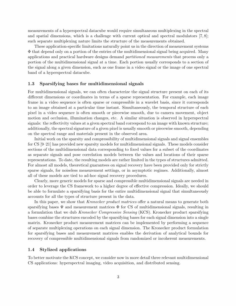
Several different extensions exist for the construction of D-D wavelets as a Kronecker product of1-D wavelet functions [34–36]. In each case, a D-D wavelet is obtained from the Kronecker productof D 1-D wavelets: ψi1,j1,...,iD,jD = ψi1,j1 ⊗ . . . ⊗ ψiD,jD . Different bases for the multidimensionalspace can then be obtained through the use of appropriate combinations of 1-D wavelets in theKronecker product. For example, isotropic wavelets arise when the same scale i = i1 = . . . = iD isselected for all wavelet functions involved, while anisotropic wavelets force a fixed factor betweenany two scales, i.e. ad,d′ = id/id′ , 1 ≤ d, d′ ≤ D. Additionally, hyperbolic wavelets result when norestriction is placed on the scales i1, . . . , iD. Therefore, a hyperbolic wavelet basis for RN1⊗. . .⊗RND

is obtained as the Kronecker product of the individual wavelet bases for RNd , 1 ≤ d ≤ D. In thesequel, we identify the isotropic, anisotropic, and hyperbolic wavelet bases as ΨI , ΨA, and ΨH ,

12

(a) (b) (c)

Figure 2: Example basis elements from 2-D wavelet bases. In each case, green (light) pixels represent zeros,while blue and red (dark) pixels represent large positive and negative values, respectively. (a) Isotropicwavelets have the same degree of smoothness on all dimensions, and are obtained from the Kronecker productof two 1-D wavelets of the same scale; (b) Anisotropic wavelets have different degrees of smoothness in eachdimension, but with a constant ratio, and are obtained from the Kronecker product of two 1-D waveletsat ratio-matching scales; (c) Hyperbolic wavelets have different degrees of smoothness in each dimensionwithout restrictions and are obtained from the Kronecker product of two 1-D wavelets of all scales.

respectively; example basis elements for each type of multidimensional wavelet basis are shown inFig. 2.

4.2 Isotropic Besov spaces

Isotropic wavelets have been popularized by their suitability for analysis of 2-D signals (images).Significant study has been devoted to identify the types of signals that are sparse or compressiblein an isotropic wavelet basis. A fundamental result in this direction states that the discretizationsof signals in isotropic Besov spaces are compressible in an isotropic wavelet basis using a sufficientlysmooth wavelet function. Such signals have the same degree of smoothness in all dimensions. Webegin by providing a brief formal definition of Besov spaces; see [35–37] for details.

We define the directional derivative of f in the direction h as (∆hf)(t) := f(t + h) − f(x),with higher-degree derivatives defined as (∆m

h f)(t) := (∆h(∆m−1h f))(t), m ≥ 2. Here and later we

define (∆hf)(t) = 0 if t + h /∈ ΩD. For r ∈ R+, m ∈ N and 0 < p < ∞, we define the modulus ofsmoothness as

ωm(f, r,ΩD)p = sup|h|≤r

‖∆mh f‖p,ΩD .

It is easy to see that ωm(f, r,ΩD)p → 0 as r → 0; smoother functions have faster decay in thisasymptotic behavior.

A signal can be classified according to its smoothness simply by imposing conditions on therate of decay of its moduli of smoothness. The resulting classes are known as Besov spaces. ABesov space Bs

p,q contains D-D functions that have (roughly speaking) s derivatives in Lp(ΩD);

this smoothness is measured by the rate of decay of the modulus of smoothness as a function of

13

the step size r. The Besov quasi-seminorm is then defined as

|f |Bsp,q

=

(∫ 1

0

[r−sωm(f, r,ΩD)p

]q drr

)1/q

.

Here the parameter q provides finer distinctions of smoothness. Thus, we say that a signal f ∈ Bsp,q

if it has finite Besov norm, defined as ‖f‖Bsp,q

= ‖f‖p + |f |Bsp,q.

Similarly to the discrete signal case, we define the best K-term approximation error in the basisΨ as

σK(f,Ψ)p = min

‖f − g‖p, g =

K∑k=1

cjψik , ψik ∈ Ψ for each i = 1, . . . ,K

.

Such isotropic wavelet-based nonlinear approximations provide provable decay rates for the approx-imation error.

Theorem 4.1 [37] If the scaling function ν ∈ Bsp,q, ν has at least s vanishing moments, and

f ∈ Brp,q, with r ≥ D/p−D/2 and 0 < r < s, then σK(f,ΨI)p < CK−r.

In words, Theorem 4.1 states that Besov-smooth signals are compressible in a sufficiently smoothisotropic wavelet transform.

4.3 Anisotropic Besov spaces

In many applications outside of natural image processing, the type of structure present is differentin each of the signal’s dimensions [12, 14, 38, 39]. For example, a video sequence has differentdegrees of smoothness in its spatial and temporal dimensions, while a hyperspectral datacubecan have different degrees of smoothness in the spatial and spectral dimensions. In these cases,anisotropic and hyperbolic wavelets can be used to achieve sparse and compressible representationsfor signals of this type. Similarly to isotropic Besov spaces, signals in anisotropic Besov spaceshave discretizations that are compressible in an anisotropic wavelet basis. We first provide a formaldefinition of anisotropic Besov spaces, which closely mirrors that of isotropic Besov spaces, exceptthat the smoothness in each dimension is specified separately.

We define the d-directional derivative of f as (∆h,df)(t) := f(t+hed)− f(t), 1 ≤ d ≤ D, whereed is the dth canonical vector, i.e., its dth entry is one and all others are zero. This corresponds tothe standard directional derivative in which the direction h is a multiple of the canonical vectored. We also define higher-degree directional derivatives as (∆m

h,df)(t) := (∆h,d(∆m−1h,d f))(t), m ≥ 2.

For r ∈ R+, md ∈ N and 0 < p <∞, we define the d-directional moduli of smoothness as

ωmd,d(f, r,ΩD)p = sup

|h|≤r‖∆md

h,df‖p,ΩD .

By defining the anisotropy parameter s = (s1, . . . , sD), we define the anisotropic Besov quasi-seminorm as [35, 36]

|f |Bsp,q

=

(∫ 1

0

[D∑d=1

r−sdωmd,d(f, r,ΩD)p

]qdr

r

)1/q

.

Thus, we say that a signal f ∈ Bsp,q if it has finite anisotropic Besov norm, defined as ‖f‖Bs

p,q=

‖f‖p + |f |Bsp,q.

14

An anisotropic Besov space Bsp,q contains functions of D continuous variables that have (roughly

speaking) sd derivatives in Lp(Ω) for any d-section of the D-D function; once again, the parameter qprovides finer distinctions of smoothness. An example is a multidimensional signal that is expressedas the Kronecker product of individual signals that are compressible in wavelet bases.

We now study the conditions for compressibility of a signal in an anisotropic wavelet basis as afunction of the smoothness of the signal in its different dimensions. We will observe that the rate ofdecay for the wavelet coefficients will depend on the characteristics of the anisotropic Besov space inwhich the signal lives. Some conditions must be imposed on the wavelets used for compressibility.We denote by ν = νi,ji,j the family of scaling functions for each scale j and offset i.

Definition 4.1 A scaling function family ν is Bsp,q-smooth, s > 0 (i.e. sd > 0, 1 ≤ d ≤ D), if

for some (m1, . . . ,mD) > s, for each i1, . . . , iD ∈ ND0 and for a finite constant C > 0 there existjd ∈ N0, 0 ≤ jd < 2id, 1 ≤ d ≤ D such that for each 0 ≤ jd < 2id, d = 1, . . . , D, and k ∈ N0,

ωmd,d(νi1,j1,...,iD,jD , 2−k,ΩD)p < Cωmd,d(νi1,j1,...,iD,jD , 2

−k,ΩD)p,

and

|νi1,j1,...,iD,jD |Bsp,q< C2(i1+...+iD)(1/2−1/p)

D∑d=1

2idsd .

It can be shown that the scaling functions formed from tensor or Kronecker products of regular1-D scaling functions νi1,j1,...,iD,jD = νi1,j1 ⊗ . . . ⊗ νiD,jD has this smoothness property when thecomponent scaling functions are smooth enough [35, 36]. This condition suffices to obtain resultson approximation rates for the different types of Kronecker product wavelet bases. The followingtheorem is an extension of a result from [36] to the D-D setting, and is proven in [40, Appendix K].

Theorem 4.2 Assume the scaling function ν that generates the anisotropic wavelet basis ΨA withanisotropy parameter s = (s1, . . . , sD) is Bs

p,q-smooth and f ∈ Brp,q, with r = (r1, . . . , rD) and

0 < r < s. Define ρ = min1≤d≤D rd and

λ =D∑D

d=1 1/rd. (8)

If ρ > D/p + D/2 then the approximation rate for the function f in an isotropic wavelet basis isσK(f,ΨI)p < CK−ρ. Similarly, if λ > D/p+D/2, then the approximation rate for the function fin both an anisotropic and a hyperbolic wavelet basis is σK(f,ΨA)p < CAK

−λ and σK(f,ΨH)p <CHK

−λ.

To give some perspective to this theorem, we study two example cases: isotropy and extremeanisotropy. In the isotropic case, all the individual rates rd = r, 1 ≤ d ≤ D, and the approximationrate under anisotropic and hyperbolic wavelets matches that of isotropic wavelets: λ = ρ = r. Inthe extreme anisotropic case, we have that one of the approximation rates is much smaller than allothers: re rd for all e 6= d. In contrast, in this case we obtain a rate of approximation underanisotropic and hyperbolic wavelets of λ ≈ Dre, which is D times larger than the rate for isotropicwavelets, ρ = re. Thus, the approximation rate with anisotropic and hyperbolic wavelets is in therange λ ∈ [1, D] min1≤d≤D rd. We also note the dependence of the result on the dimensionality ofthe signal: as D increases, the requirements on the smoothnesses ρ, λ of the function f becomemore strict.

15

The disadvantage of anisotropic wavelets, as compared with hyperbolic wavelets, is that theymust have an anisotropy parameter that matches that of the anisotropic smoothness of the signal inorder to achieve the optimal approximation rate [35]. Additionally, the hyperbolic wavelet basis isthe only one out of the three basis types described that can be expressed as the Kronecker productof lower dimensional wavelet bases. Therefore, we use hyperbolic wavelets in the sequel and in theexperiments of Section 5.

4.4 Performance of KCS with multidimensional hyperbolic wavelet bases

Since KCS uses Kronecker product matrices for measurement and compression of multidimensionalsignals, it is possible to compare the rates of approximation that can be obtained by using inde-pendent measurements of each d-section of the multidimensional signal against those obtained byKCS. The following Theorem is obtained by amalgamating the results of Theorems 2.1, 2.3, and 4.2and Lemma 3.1.

Theorem 4.3 Assume that a D-D signal x ∈ RN1×...×ND is the sampled version of a continuous-time signal f ∈ Bs

1,q, with s = s1, . . . , sD, under the conditions of Theorem 4.2 with p = 1. Inparticular, x has sd-compressible d-sections in sufficiently smooth wavelet bases Ψd, 1 ≤ d ≤ D.Denote by Φd, 1 ≤ d ≤ D a set of CS measurement bases that can be applied along each dimensionof x. If M total measurements are obtained using a random subset of the columns of Φ1⊗ . . .⊗ΦD,then with high probability the recovery error from these measurements has the property

‖x− x‖2 ≤ C

(M√

N∏Dd=1 µ(Φd,Ψd)

)−β, (9)

where β = D2∑D

d=1 1/sd+ 1

4 , while the recovery from M measurements equally distributed among the

eth dimension of the signal using the basis Φ1 ⊗ . . .⊗ Φe−1 ⊗ Φe+1 ⊗ . . .⊗ ΦD on each 1, . . . , e−1, e+ 1, . . . , D-section of x has the property

‖x− x‖2 ≤ CN1/2e

(M√

N/Ne∏d6=e µ(Φd,Ψd)

)−βe, (10)

where βe = D−12∑

d 6=e 1/sd+ 1

4 .

Proof sketch. For recovery we pair the Kronecker product measurement matrix ΦP := Φ1 ⊗. . .⊗ ΦD with the hyperbolic wavelet basis ΨH = Ψ1 ⊗ . . .⊗ΨD. From Lemma 3.1, we have thatthe mutual coherence of these two bases is µ(ΦP ,ΨH) =

∏Dd=1 µ(Φd,Ψd). Plugging this value into

Theorem 2.3, the number of measurements needed to achieve the RIP having δ2K =√

2 − 1 withhigh probability is

M = CMK√N

D∏d=1

µ(Φd,Ψd) log(tK logN) log2(K). (11)

The RIP, in turn, guarantees that the recovery error obeys ‖x−x‖2 = ‖θ− θ‖2 ≤ CK−1/2‖θ−θK‖1,as given in Theorem 2.1, with θ and θ denoting the coefficients of x and x, respectively; note that

16

the output of the recovery algorithms (3-4) is given by θ, with x = ΨH θ. The approximation erroris then bounded using Theorem 4.2 by ‖θ − θK‖1 = σK(f,ΨH)1 ≤ CHK−λ, where we use the factthat θ is the discrete wavelet transform coefficient vector for the vector x, which itself contains Nuniform samples of the continuous signal f ∈ Bs

1,q. We therefore obtain

‖x− x‖2 ≤ CCHK−λ−1/2. (12)

At this point we solve for K in (11) to obtain

CKK2 ≥ K log(tK logN) log2(K) =

M

CM√N

D∏d=1

µ(Φd,Ψd)−1,

K ≥ C ′K(M√N

)1/2 D∏d=1

µ(Φd,Ψd)−1/2.

Plugging into (12), we obtain

‖x− x‖2 ≤ CCHC ′λ+1/2K

(M√N

)−λ/2−1/4 D∏d=1

µ(Φd,Ψd)λ/2+1/4.

By noticing that β = λ/2 + 1/4, we have obtained (9).The proof of (10) proceeds similarly by partitioning along the eth dimension and adjusting the

number of measurements per 1, . . . , e−1, e+ 1, . . . , D-section to M/Ne, so that the term M/√N

in (9) is replaced by (M/Ne)/√N/Ne = M/

√NNe, introducing a new multiplicative term N

βe/2e .

A triangle inequality to assemble the error for the entire D-D signal from the different e-sectionsintroduces a new additional factor of

√Ne.

To put Theorem 4.3 in perspective, we study the bases and the exponents of the bounds sepa-rately. With regards to the bases, the denominators in (9)–(10) provide a scaling for the numberof measurements needed to achieve a target recovery accuracy. This scaling is dependent on themeasurement matrices via mutual coherences; the denominators take values in the ranges [1,

√N ]

and [1,√N/Ne], respectively. With regards to the exponents, the rates of decay for the recovery

error match those of the signal’s compressibility approximation error rates λ from (8) for the entiresignal and its partitions, respectively. The error decay rate for KCS recovery is higher than that forindependent recovery from partitioned measurements when se >

D−1∑d 6=e 1/sd

, i.e., when the compress-

ibility exponent of the e-sections is larger than the harmonic mean of the compressibility exponentsof all other sections. Thus, KCS provides the most significant improvement in the error rate ofdecay when the measurement partitioning is applied along the dimension(s) that feature highestcompressibility or smoothness. Note also the

√Ne cost in (10) of partitioning measurements, which

comes from the triangle inequality.

5 Experimental Results

In this section, we perform experiments to verify the compressibility properties of two differentclasses of signals in a Kronecker product wavelet basis. We also perform KCS sparse recovery exper-iments that illustrate the advantages of KCS over standard CS schemes. For the multidimensional

17

signals, in addition to synthetic data, we choose 3D hyperspectral imagery and video sequences,since they can be compressed effectively by well-studied, albeit data-dependent, compression algo-rithms (the Karhunen-Loeve transform (KLT) and motion compensation, respectively). Our intentis to see how close we can come to this nonlinear compression performance using the simpler linearKronecker product wavelet basis for compression and CS recovery. We will also experimentallyverify the tradeoffs provided in Sections 3 and 4 and contrast the recovery performance to thatreached by integrating such task-specific compression schemes to distributed CS recovery.

The experiments use the basis pursuit solvers from [41] and [42] for the hyperspectral and videodata, respectively. The experiments were executed on a Linux workstation with an Intel Xeon CPUat 3.166 GHz and 4 GB of memory. A Matlab toolbox containing the scripts that generate theresults and figures provided in this section is available for download at http://dsp.rice.edu/kcs.Additional experimental results are also available in [40].

5.1 Empirical Performance of KCS

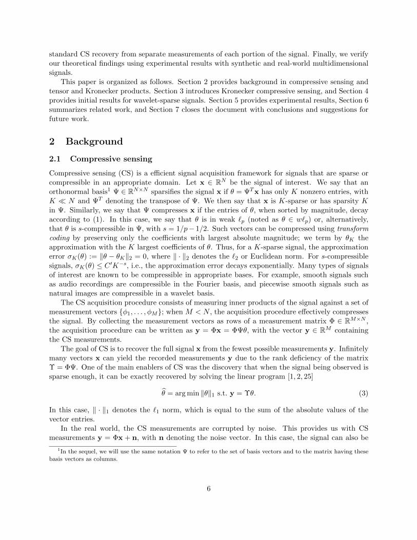
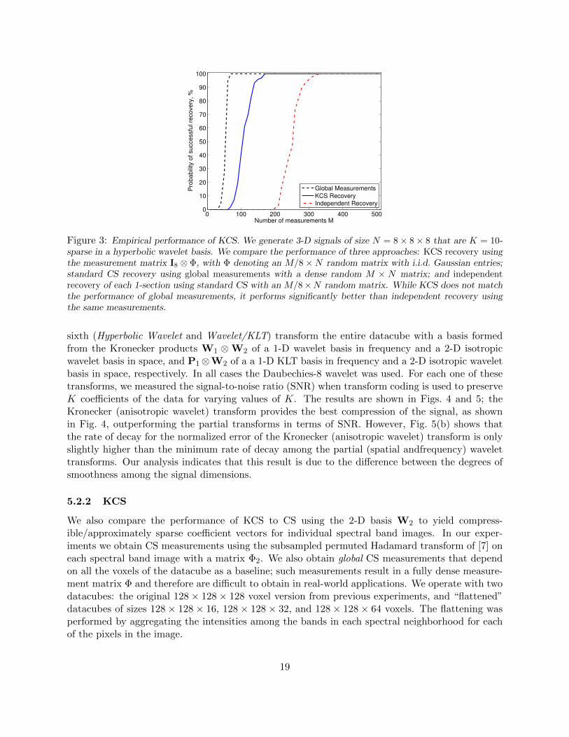
Our first experiment considers synthetically generated signals of size N = 8×8×8 that are K = 10-sparse in a Kronecker product (hyperbolic) wavelet basis and compares three CS recovery schemes:the first uses a single recovery from dense, global measurements; the second uses a single KCSrecovery from the set of measurements obtained independently from each 8× 8 1-section; and thethird one uses independent recovery of each 8× 8 1-section from its individual measurements. Welet the number of measurements M vary from 0 to N with the measurements evenly split amongthe 1-sections in the independent and KCS recovery cases. For each value of M , we average 100iterations by generating K-sparse signals x with independent and identically distributed (i.i.d.)Gaussian entries and with support following a uniform distribution among all supports of size K,and generating measurement matrices with i.i.d. Gaussian entries. We then measure the probabilityof successful recovery for each value of M , where a success is declared if the signal estimate x obeys‖x− x‖2 ≤ 10−3‖x‖2. The results are shown in Fig. 3, which shows that KCS outperforms separatesection-by-section recovery while achieving lower success probabilities than recovery from globalmeasurements. In fact, the measurement-to-sparsity ratio M/K required for 95% success rate are6, 15, and 30 for global measurements, KCS, and independent recovery, respectively.

5.2 Hyperspectral data

5.2.1 Compressibility

We first evaluate the compressibility of a real-world hyperspectral datacube using independentspatial and spectral sparsifying bases and compare it with a Kronecker product basis. The datacubefor this experiment is obtained from the AVIRIS Moffett Field database [43]. A N = 128×128×128voxel portion is used. We then process the signal through six different transforms. The first three(Space, Frequency Wavelet, Frequency KLT) perform transforms along a subset of the dimensionsof the data (a 1-D wavelet basis W1 for the spectral dimension, a 2-D wavelet basis W2 for thespatial dimensions, and a 1-D KLT basis2 P1 for the spectral dimension, respectively). The fourth(Isotropic Wavelet) transforms the entire datacube with a 3-D isotropic wavelet basis. The fifth and

2A KLT basis is learned from a datacube of the same size extracted from a different spatial region of the originalAVIRIS dataset [20, 44, 45]. The resulting transformation provides a linear approximation scheme that preserves thecoefficients for the most significant principal components, rather than the nonlinear approximation scheme used insparse approximation.

18

0 100 200 300 400 5000

10

20

30

40

50

60

70

80

90

100

Number of measurements M

Pro

babili

ty o

f successfu

l re

covery

, %

Global Measurements

KCS Recovery

Independent Recovery

Figure 3: Empirical performance of KCS. We generate 3-D signals of size N = 8× 8× 8 that are K = 10-sparse in a hyperbolic wavelet basis. We compare the performance of three approaches: KCS recovery usingthe measurement matrix I8 ⊗ Φ, with Φ denoting an M/8×N random matrix with i.i.d. Gaussian entries;standard CS recovery using global measurements with a dense random M × N matrix; and independentrecovery of each 1-section using standard CS with an M/8×N random matrix. While KCS does not matchthe performance of global measurements, it performs significantly better than independent recovery usingthe same measurements.

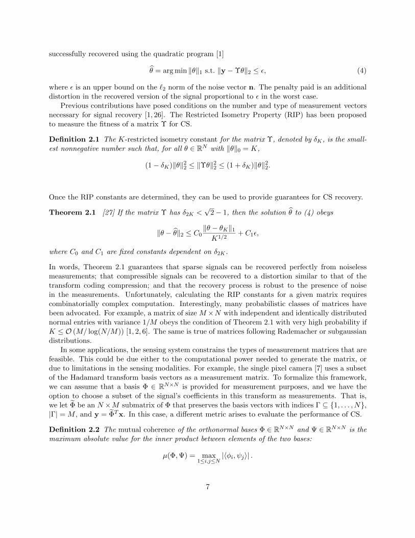
sixth (Hyperbolic Wavelet and Wavelet/KLT) transform the entire datacube with a basis formedfrom the Kronecker products W1 ⊗W2 of a 1-D wavelet basis in frequency and a 2-D isotropicwavelet basis in space, and P1⊗W2 of a a 1-D KLT basis in frequency and a 2-D isotropic waveletbasis in space, respectively. In all cases the Daubechies-8 wavelet was used. For each one of thesetransforms, we measured the signal-to-noise ratio (SNR) when transform coding is used to preserveK coefficients of the data for varying values of K. The results are shown in Figs. 4 and 5; theKronecker (anisotropic wavelet) transform provides the best compression of the signal, as shownin Fig. 4, outperforming the partial transforms in terms of SNR. However, Fig. 5(b) shows thatthe rate of decay for the normalized error of the Kronecker (anisotropic wavelet) transform is onlyslightly higher than the minimum rate of decay among the partial (spatial andfrequency) wavelettransforms. Our analysis indicates that this result is due to the difference between the degrees ofsmoothness among the signal dimensions.

5.2.2 KCS

We also compare the performance of KCS to CS using the 2-D basis W2 to yield compress-ible/approximately sparse coefficient vectors for individual spectral band images. In our exper-iments we obtain CS measurements using the subsampled permuted Hadamard transform of [7] oneach spectral band image with a matrix Φ2. We also obtain global CS measurements that dependon all the voxels of the datacube as a baseline; such measurements result in a fully dense measure-ment matrix Φ and therefore are difficult to obtain in real-world applications. We operate with twodatacubes: the original 128 × 128 × 128 voxel version from previous experiments, and “flattened”datacubes of sizes 128 × 128 × 16, 128 × 128 × 32, and 128 × 128 × 64 voxels. The flattening wasperformed by aggregating the intensities among the bands in each spectral neighborhood for eachof the pixels in the image.

19

0 1 2

x 104

0

1

2

3

x 105

Coeff. mag.

Count

0 1 2

x 104

0

5

10

x 105

Coeff. mag.

Co

un

t

0 1 2

x 104

0

5

10

15

x 105

Coeff. mag.

Co

un

t

0 1 2

x 104

0

5

10

15

x 105

Coeff. mag.

Co

un

t

(a) (b) (c) (d)

Figure 4: Examples of transform coding of a hyperspectral datacube of size 128 × 128 × 128. (a) Original data;(b) Coefficients in a 1-D wavelet basis W1 applied at each pixel in the spectral domain; (c) Coefficients in a 2-Disotropic wavelet basis W2 applied at each pixel in the spatial domain; (d) Coefficients in a Kronecker product basisW1 ⊗ W2. The top row shows the datacube or coefficients flattened to 2-D by concatenating each spectral band’simage, left to right, top to bottom. In (b-d), blue (dark) pixels represent coefficients with small magnitudes. Thebottom row shows histograms for the coefficient magnitudes, showing the highest concentrations of small coefficientsfor the Kronecker product basis.

Figure 6 shows the recovery error for each datacube from several different recovery setups: In-dependent recovery operates on each spectral band independently with the measurement matrix Φ2

using the basis W2 to sparsify each spectral band. KCS employs the Kronecker product measure-ment matrix I⊗Φ2 to perform joint recovery. We test two different Kronecker product sparsifyingbases: KCS-Wavelet uses a Kronecker products of wavelet bases W1 ⊗W2, and KCS-KLT uses aKronecker product P1 ⊗W2 of a KLT basis P1 in the spectral dimension and a 2-D wavelet basisW2 in the spatial dimensions. We also show results using these two Kronecker product sparsifyingbases together with Global measurements Φ that depend on all voxels of the datacube.

We see an improvement on recovery from distributed over global measurements when the numberof measurements M obtained for each band is small; as M increases, this advantage vanishes due tothe availability of sufficient information. We also see that the performance of independent recoveryimproves as the number of spectral bands increases and eventually matches the performance of

20

0 2 4 6 8 10

x 104

0

5

10

15

20

25

30

35

40

Number of coefficients, K

Tra

nsfo

rm c

odin

g c

om

pre

ssio

n S

NR

, dB

Wavelet/KLTHyperbolic WaveletIsotropic WaveletSpace WaveletFrequency KLTFrequency Wavelet

100

102

104

10−2

10−1

Number of coefficients, K (log scale)

No

rma

lize

d e

rro

r m

ag

nitu

de

(lo

g s

ca

le),

dB

Hyperbolic WaveletWavelet/KLTIsotropic WaveletSpace WaveletFrequency WaveletFrequency KLT

(a) (b)

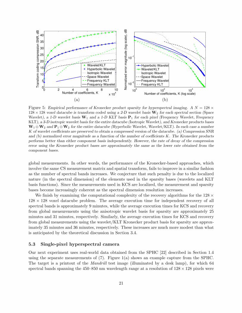
Figure 5: Empirical performance of Kronecker product sparsity for hyperspectral imaging. A N = 128 ×128× 128 voxel datacube is transform coded using a 2-D wavelet basis W2 for each spectral section (SpaceWavelet), a 1-D wavelet basis W1 and a 1-D KLT basis P1 for each pixel (Frequency Wavelet, FrequencyKLT), a 3-D isotropic wavelet basis for the entire datacube (Isotropic Wavelet), and Kronecker products basesW1⊗W2 and P1⊗W2 for the entire datacube (Hyperbolic Wavelet, Wavelet/KLT). In each case a numberK of wavelet coefficients are preserved to obtain a compressed version of the datacube. (a) Compression SNRand (b) normalized error magnitude as a function of the number of coefficients K. The Kronecker productsperforms better than either component basis independently. However, the rate of decay of the compressionerror using the Kronecker product bases are approximately the same as the lower rate obtained from thecomponent bases.

global measurements. In other words, the performance of the Kronecker-based approaches, whichinvolve the same CS measurement matrix and spatial transform, fails to improve in a similar fashionas the number of spectral bands increases. We conjecture that such penalty is due to the localizednature (in the spectral dimension) of the elements used in the sparsity bases (wavelets and KLTbasis functions). Since the measurements used in KCS are localized, the measurement and sparsitybases become increasingly coherent as the spectral dimension resolution increases.

We finish by examining the computational complexity of the recovery algorithms for the 128×128 × 128 voxel datacube problem. The average execution time for independent recovery of allspectral bands is approximately 9 minutes, while the average execution times for KCS and recoveryfrom global measurements using the anisotropic wavelet basis for sparsity are approximately 25minutes and 31 minutes, respectively. Similarly, the average execution times for KCS and recoveryfrom global measurements using the wavelet/KLT Kronecker product basis for sparsity are approx-imately 35 minutes and 36 minutes, respectively. These increases are much more modest than whatis anticipated by the theoretical discussion in Section 3.4.

5.3 Single-pixel hyperspectral camera

Our next experiment uses real-world data obtained from the SPHC [22] described in Section 1.4using the separate measurements of (7). Figure 1(a) shows an example capture from the SPHC.The target is a printout of the Mandrill test image (illuminated by a desk lamp), for which 64spectral bands spanning the 450–850 nm wavelength range at a resolution of 128× 128 pixels were

21

0.1 0.2 0.3 0.4 0.55

10

15

20

Normalized number of measurements, M/N

SN

R, dB

Kronecker KLT/GlobalKCS−KLTKronecker Wavelet/GlobalKCS−WaveletIndependent Recovery

0.1 0.2 0.3 0.4 0.55

10

15

20

Normalized number of measurements, M/N

SN

R,

dB

Kronecker KLT/GlobalKCS−KLTKronecker Wavelet/GlobalKCS−WaveletIndependent Recovery

(a) (b)

0.1 0.2 0.3 0.4 0.5

10

15

20

Normalized number of measurements, M/N

SN

R, dB

Kronecker KLT/GlobalKCS−KLTKronecker Wavelet/GlobalKCS−WaveletIndependent Recovery

0.1 0.2 0.3 0.4 0.5

8

10

12

14

16

18

20

Normalized number of measurements, M/N

SN

R,

dB

Independent RecoveryKronecker KLT/GlobalKCS−KLTKronecker Wavelet/GlobalKCS Wavelet

(c) (d)

Figure 6: Empirical performance of KCS and standard CS for hyperspectral imaging for datacubes of sizes(a) N = 128×128×16, (b) N = 128×128×32, (c) N = 128×128×64, and (d) N = 128×128×128 voxels.Each datacube is recovered from CS measurements of each spectral band image from a matrix Φ2 usingseparate CS recovery of each spectral band image using the measurement matrix Φ2 and a sparsifying 2-Dwavelet basis W2 (Independent Recovery); joint CS recovery of all spectral bands using a global measurementmatrix Φ and sparsifying Kronecker product bases W1⊗W2 and P1⊗W2 (Kronecker Wavelet/Global andKronecker KLT/Global, respectively); and KCS recovery using the measurement matrix I ⊗ Φ2 and thesparsifying bases W1 ⊗W2 and P1 ⊗W2 (KCS-Wavelet and KCS-KLT, respectively). Recovery usingthe Kronecker product sparsifying bases outperforms separate recovery. Additionally, there is an advantageto applying distributed rather than global measurements when the number of measurements M is low.Furthermore, as the resolution of the spectral dimension increases, the Kronecker sparsity and Kroneckermeasurement bases become increasingly coherent, hampering the performance of joint recovery techniques.

obtained. In Fig. 1(b), each spectral band was recovered separately. In Fig. 1(c), the spectral bandswere recovered jointly with KCS using the measurement structure of (7) and a hyperbolic waveletbasis. The results show a considerable quality improvement over independent recovery, particularlyfor spectral frames with low signal power.

22

200 400 600 800 10005

10

15

20

Number of coefficients, KCom

pre

ssio

n S

NR

, dB

KroneckerIsotropicSpace

(a) (b)

Figure 7: (a) Example cropped frame from the QCIF-format Foreman video sequence, size 128× 128. (b)Empirical performance of Kronecker product sparsifying basis for transform coding of the Foreman videosequence, N = 128× 128× 128 = 221 voxels. We subject it to transform coding using a spatial 2D waveletbasis W2 for each frame (Space), a 3-D Isotropic wavelet bases W3 for the entire sequence, and a Kroneckerproduct basis W1 ⊗W2 for the entire sequence. The Kronecker product performs better in distortion thanthe alternative bases.

5.4 Video data

5.4.1 Compressibility

We evaluate the compressibility of video sequences in an independent spatial (per frame) sparsifyingbasis and compare it with a standard isotropic wavelet basis and a Kronecker product wavelet basis.We use the standard Foreman video sequence, which we crop around the center to have frames ofsize 128 × 128 pixels, as shown in Fig. 7(a). We select 128 frames to obtain a signal of lengthN = 221 samples. We then process the signal through three different transforms: the first (Space)applies the 2-D wavelet basis W2 along the spatial dimensions of the data, with no compressionon the temporal dimension; the second (Isotropic) applies the standard isotropic 3D wavelet basisW3 on the entire video sequence, and the third (Kronecker) transforms the entire sequence withthe Kronecker product basis W1 ⊗W2, providing a hyperbolic wavelet basis. For each one ofthese transforms, we measured the compression signal-to-noise ratio (SNR) when transform codingis used to preserve K coefficients of the data for varying values of K. The results are shown inFig. 7(b) and closely resemble those obtained for hyperspectral data. Additionally, the Kroneckerproduct outperforms isotropic wavelets due to the difference in smoothness between the temporaland spatial dimensions.

5.4.2 KCS

We compare the performance of KCS to that of CS using the low-dimensional basis W2 to yieldcompressible/approximately sparse coefficient vectors for individual frames. In our experimentswe obtain CS measurements on each video frame using a matrix Φ2 obtained from a subsampledpermuted Hadamard transform [7]. For KCS we use a single Kronecker product measurementmatrix as shown in (7), while for standard CS we perform independent recovery of each frameusing the measurement matrix Φ2. We also use a global CS measurement matrix Φ, where themeasurements depend on all the pixels of the video sequence, as a baseline. Figure 8 shows therecovery error from several different setups. Independent recovery uses CS on each video frameindependently with the sparsifying basis W2. KCS employs the Kronecker product measurementand sparsity/compressibility transform matrices I⊗Φ2 and W1⊗W2, respectively, to perform jointrecovery of all frames. We also show results using the Kronecker product sparsity/compressibility

23

0.1 0.2 0.3 0.4 0.5

20

25

30

35

Normalized number of measurements, M/N

PS

NR

, d

B

Kronecker/GlobalKCSIndependentMotion Compensation

Figure 8: Empirical performance of KCS for the Foreman video sequence. We recover the video sequenceusing independent recovery of each frame using a measurement matrix Φ2 and sparsifying basis W2; inde-pendent block-based CS and recovery with motion compensation post-processing on individual frames withGOP size 8, block-wise random measurement matrix and block-wise 2-D discrete cosine transform (DCT)sparsifying basis; KCS with measurement matrix I⊗Φ2 and sparsifying basis W1 ⊗W2; and joint recoveryof all frames in the sequence using the Kronecker sparsifying basis W1 ⊗W2 and a global measurementmatrix Φ. While KCS does not perform as well as CS using global measurements, it shows an improve-ment over separate recovery of each frame in the video sequence using the same measurements. The motioncompensation-aided approach outperforms the generic approaches.

transform basis W1 ⊗W2 paired with the Global measurement matrix Φ.Finally, we compare the above linear approaches to a state-of-the-art recovery algorithm based

on nonlinear motion compensated block-based CS (MC-BCS) [21]. In MS-BCS disjoint blocks ofeach video frame are separately measured using both a random measurement matrix and a 2-Ddiscrete cosine transform (DCT) for sparsity/compressibility. The blocks of a reference frame arerecovered using standard CS recovery algorithms. MC-BCS then calculates measurements for thedifference with the subsequent frame by subtracting the corresponding measurement vectors, andrecovers the blocks of the frame difference using standard CS algorithms. The frame differenceis then refined using motion compensation (MC); the MC output is used to obtain a new framedifference and the process is repeated iteratively for each frame, and again for each subsequentframe in the group of pictures (GOP). Further refinements enable additional improvements in thequality of the recovered video sequence. A toolbox implementing MC-BCS was made available whilethis paper was under review [21]. We set the GOP size to 8 and use blocks of size 16×16, followingthe parameter values of the toolbox implementation. In contrast to [21], we set the number ofmeasurements for each of the frames to be equal to match the KCS partitioning of measurements.

The Foreman sequence features camera movement, which is reflected in sharp changes in thevalue of each pixel across frames. We see, once again, that while KCS does not perform as wellas CS with global measurements, it does outperform independent recovery of each frame in thesequence operating on the same measurements. Furthermore, the quality of KCS recovery comeswithin 5 dB of that of MC-BCS, which may be surprising considering that the motion compensationperformed in MC-BCS is especially designed for video coding and compression.

The average execution time for independent recovery of all video frames is approximately 13seconds. In contrast, the average execution times for KCS and recovery from global measurements

24

using the anisotropic wavelet basis for sparsity are approximately 104 minutes and 220 minutes,respectively. These results agree with the discussion in Section 3.4, since the computational timeof KCS recovery is increased by a factor of about 128× 3 = 384 over that of independent recovery.The average execution time for motion compensation-aided recovery is 34 minutes.

6 Related work

Prior work for CS of multidimensional signals focuses on the example applications given in thispaper – hyperspectral imaging [11, 44–46] and video acquisition [10, 12–15, 17, 20, 21] – with lim-ited additional work dealing with applications such as sensor networks [9, 18, 19] and confocalmicroscopy [16]. These formulations employ measurement schemes that act on a partition of thedata x1, . . . ,xJ, such as frames of a video sequence. For those cases, individual measurementvectors y1, . . . ,yJ are obtained using a set of matrices Φ1, . . . ,ΦJ [9–17, 20, 21], resulting inthe measurement matrix structure of (7). While global measurements that depend on the entire setof data have been proposed [8, 10, 16, 20], practical architectures that provide such measurementsare rare [8]. Similarly, partitioned measurements have been proposed for CS of low-dimensionalsignals for computational purposes [29, 30, 47]. Below we contrast the signal model and algorithmsused in these approaches with those used in KCS.

Several frameworks have been proposed to encode the sparse structure of multidimensional sig-nals. The most significant class of structures link the signals through overlap of nonzero coefficientvalues and locations. That is, there exists a matrix P of size JN × D with binary entries (0 or1) and a vector Θ of length D such that x = (I ⊗ Ψ)PΘ. The vector Θ encodes the correlationsand has length lower than the sum of the sparsities of the signals [9, 13, 15, 18, 19]. Such matricesare very rigid in the kinds of structures they can represent; in KCS we can represent a variety ofmultidimensional structures by using sparse representations on each of the signal dimensions.

Kronecker product matrices have been proposed for use as sparsifying bases in CS for certainspatiotemporal signals [12, 14, 20]. In other cases, specialized compression bases are combined withspecially tailored recovery algorithms [11, 15, 17, 20, 21]; a prime example is motion compensationfor video sequences [15, 21]. While such tailored algorithms often provide superior performance,they seldom come with theoretical tractability and performance guarantees. In contrast, KCS canuse a variety of standard CS recovery algorithms and preserves their guarantees, since it relies onstandard matrices for measure and sparsity/compressibility transforms. Standard sparsifying basesfor CS, such as multidimensional isotropic wavelets, suffice only for very specific classes of signalsthat do feature similar degrees of smoothness along each of their dimensions [10, 16]; KCS usinghyperbolic wavelet bases can be applied to signals with different degrees of smoothness in each oftheir dimensions.

In transform coding, anisotropic and hyperbolic wavelet bases have been proposed for compres-sion of hyperspectral datacubes and video sequences [20, 38, 46]; however, to date no mathematicalanalysis of their performance has been provided. Kronecker products involving matrices obtainedfrom principal component analysis and Karhunen-Loeve transforms have also been used for this pur-pose. However, they rely on linear low-dimensional approximations rather than nonlinear sparserepresentations [20, 44, 45]; thus, the approaches are more data-dependent and more difficult togeneralize among different datasets.

Finally, we are aware of two initial studies on the properties of Kronecker product matrices forCS [29, 30, 32]. Our study of their mutual coherence properties matches that independently obtained

25

in [29, 30], while [32] provides only a lower bound for their restricted isometry constants; we haveprovide an upper bound based on the properties of the eigendecomposition of their submatrices.

7 Conclusions and Further Work

In this paper we have developed the concept of Kronecker compressive sensing and presented initialanalytical and experimental results on its performance. Out theoretical framework is motivatedby new sensing applications that acquire multidimensional signals in a progressive fashion, as wellas by settings where the measurement process is distributed, such as sensor networks and arrays.We have also provided analytical results for the recovery of signals that live in anisotropic Besovspaces, where there is a well-defined relationship between the degrees of compressibility obtainedusing lower-dimensional wavelet bases on portions of the signal and multidimensional anisotropicwavelet bases on the entire signal. Furthermore, because the formulation follows the standardCS approach of single measurement and sparsifying matrices, standard recovery algorithms thatprovide provable guarantees can be used; this obviates the need to develop ad-hoc algorithms toexploit additional signal structure.

Further work remains in finding additional signal classes for which the use of multidimensionalstructures provides an advantage during compression. Some promising candidates include modula-tion spaces, which contain signals that can be compressed using Wilson and brushlet bases [48, 49].Our KCS framework also motivates the formulation of novel structured representations using spar-sifying bases in applications where transform coding compression schemes have not been developed.

While we focused on hyperspectral imaging and video acquisition, there exist other interestingapplications where Kronecker product sparsifying bases and KCS are relevant. In sensor networksand arrays, sparsity-based distributed localization [24, 50, 51] obtains a sparse estimate of the vectorcontaining the samples obtained in a dictionary that contains the responses of a known source ata set of feasible locations. The sparse vector will encode the location of the source within thefeasible set. When the source signal is not known, we can assume that it is sparse in a known basisand employ a Kronecker product matrix that encodes both the propagation physics and the sparseor compressible structure of the source signal. In medical imaging, there are many applicationswhere estimates of high-dimensional data are obtained from highly undersampled measurements,including 3-D computed tomography, angiography [12], 3-D magnetic resonance imaging (MRI) [12],and functional MRI.

Acknowledgements

Thanks to Ron DeVore for many valuable discussions and for pointing us to [35, 36] and to JustinRomberg for pointing us to the remark in [28]. Special thanks to Kevin Kelly, Ting Sun andDharmpal Takhar for providing experimental data for the single-pixel hyperspectral camera. Andthanks to Don Johnson, Chinmay Hegde, Jason Laska, Shriram Sarvotham, and Michael Wakin forhelpful comments. Finally, we thank the anonymous reviewers for many helpful comments.

References

[1] E. J. Candes, “Compressive sampling,” in Int. Congress of Mathematicians, Madrid, Spain,2006, vol. 3, pp. 1433–1452.

26

[2] D. L. Donoho, “Compressed sensing,” IEEE Trans. Info. Theory, vol. 52, no. 4, pp. 1289–1306,Sept. 2006.

[3] D. J. Brady, “Multiplex sensors and the constant radiance theorem,” Optics Letters, vol. 27,no. 1, pp. 16–18, Jan. 2002.

[4] J. Tropp and A. C. Gilbert, “Signal recovery from partial information via orthogonal matchingpursuit,” IEEE Trans. Info. Theory, vol. 53, no. 12, pp. 4655–4666, Dec. 2007.

[5] J. Haupt and R. Nowak, “Signal reconstruction from noisy random projections,” IEEE Trans.Info. Theory, vol. 52, no. 9, pp. 4036–4048, Sept. 2006.

[6] R. G. Baraniuk, M. A. Davenport, R. A. DeVore, and M. B. Wakin, “A simple proof of therestricted isometry property for random matrices,” Constructive Approximation, vol. 28, no.3, pp. 253–263, Dec. 2008.

[7] M. F. Duarte, M. A. Davenport, D. Takhar, J. N. Laska, T. Sun, K. F. Kelly, and R. G.Baraniuk, “Single pixel imaging via compressive sampling,” IEEE Signal Proc. Mag., vol. 25,no. 2, pp. 83–91, March 2008.

[8] A. Wagadarikar, R. John, R. Willett, and David Brady, “Single disperser design for codedaperture snapshot spectral imaging,” Applied Optics, vol. 47, no. 10, pp. B44–B51, 2008.

[9] D. Baron, M. B. Wakin, M. F. Duarte, S. Sarvotham, and R. G. Baraniuk, “Distributedcompressed sensing,” Tech. Rep. TREE-0612, Rice University Department of Electrical andComputer Engineering, Houston, TX, Nov. 2006.

[10] M. B. Wakin, J. N. Laska, M. F. Duarte, D. Baron, S. Sarvotham, D. Takhar, K. F. Kelly,and R. G. Baraniuk, “Compressive imaging for video representation and coding,” in PictureCoding Symposium, Beijing, China, Apr. 2006.

[11] R. M. Willett, M. E. Gehm, and D. J. Brady, “Multiscale reconstruction for computationalhyperspectral imaging,” in IS&T/SPIE Symposium on Electronic Imaging: Comp. Imaging,San Jose, CA, Jan. 2007.

[12] M. Lustig, D. L. Donoho, J. M. Santos, and J. M. Pauly, “Compressed sensing MRI,” IEEESignal Proc. Mag., vol. 25, no. 2, pp. 72–82, Mar. 2008.

[13] R. F. Marcia and R. M. Willett, “Compressive coded aperture video reconstruction,” inEuropean Signal Proc. Conf. (EUSIPCO), Lausanne, Switzerland, Aug. 2008.

[14] V. Stankovic, L. Stankovic, and S. Cheng, “Compressive video sampling,” in European SignalProc. Conf. (EUSIPCO), Lausanne, Switzerland, Aug. 2008.

[15] L.-W. Kang and C.-S. Lu, “Distributed compressed video sensing,” in IEEE Int. Conf. onAcoustics, Speech and Signal Proc. (ICASSP), Taipei, Taiwan, Apr. 2009, pp. 1169–1172.

[16] P. Ye, J. L. Paredes, G. R. Arce, Y. Wu, C. Chen, and D. W. Prather, “Compressive confocalmicroscopy: 3D reconstruction algorithms,” in SPIE Photonics West, San Jose, CA, Jan.2009.

27

[17] J. Y. Park and M. B. Wakin, “A multiscale framework for compressive sensing of video,” inPicture Coding Simposium, Chicago, IL, May 2009.

[18] Y. Eldar and M. Mishali, “Robust recovery of signals from a structured union of subspaces,”IEEE Trans. Info. Theory, vol. 55, no. 11, pp. 5302–5316, Nov. 2009.

[19] R. G. Baraniuk, V. Cevher, M. F. Duarte, and C. Hegde, “Model-based compressive sensing,”IEEE Trans. Info. Theory, vol. 56, no. 4, pp. 1982–2001, Apr. 2010.

[20] M Cossalter, M. Tagliasacchi, G. Valenzise, and S. Tubaro, “Joint compressive video codingand analysis,” IEEE Trans. Multimedia, vol. 12, no. 3, pp. 168–183, Apr. 2010.

[21] S. Mun and J. E. Fowler, “Residual reconstruction for block-based compressed sensing ofvideo,” in IEEE Data Compression Conf. (DCC), Snowbird, UT, Mar. 2011.

[22] T. Sun and K. F. Kelly, “Compressive sensing hyperspectral imager,” in Comp. OpticalSensing and Imaging (COSI), San Jose, CA, Oct. 2009.

[23] D. Takhar, Compressed sensing for imaging applications, Ph.D. thesis, Rice University, Hous-ton, TX, Feb. 2008.

[24] V. Cevher, M. F. Duarte, and R. G. Baraniuk, “Localization via spatial sparsity,” in EuropeanSignal Proc. Conf. (EUSIPCO), Lausanne, Switzerland, 2008.

[25] S. Chen, D. Donoho, and M. Saunders, “Atomic decomposition by basis pursuit,” SIAM J.on Sci. Comp., vol. 20, no. 1, pp. 33–61, 1998.

[26] E. J. Candes and J. Romberg, “Sparsity and incoherence in compressive sampling,” InverseProblems, vol. 23, no. 3, pp. 969–985, 2007.

[27] E. J. Candes, “The restricted isometry property and its implications for compressed sensing,”Compte Rendus de l’Academie des Sciences Series I, vol. 346, pp. 589–592, 2008.

[28] M. Rudelson and R. Vershynin, “On sparse reconstruction from Fourier and Gaussian mea-surements,” Comm. on Pure and Applied Math., vol. 61, no. 8, pp. 1025–1171, Aug. 2008.

[29] Y. Rivenson and A. Stern, “Compressed imaging with a separable sensing operator,” IEEESignal Proc. Letters, vol. 16, no. 6, pp. 449–452, June 2009.

[30] Y. Rivenson and A. Stern, “An efficient method for multi-dimensional compressive imaging,”in Comp. Optical Sensing and Imaging (COSI), San Jose, CA, Oct. 2009.

[31] R. C. Thompson, “Principal submatrices XI: Interlacing inequalities for singular values,”Linear Algebra and Appl., vol. 5, pp. 1–12, 1972.

[32] S. Jokar and V. Mehrmann, “Sparse representation of solutions of Kronecker product systems,”Linear Algebra and Appl., vol. 431, no. 12, pp. 2437–2447, Dec. 2009.

[33] S. Boyd and L. Vanderberghe, Convex Optimization, Cambridge University Press, New York,NY, 2004.

28

[34] S. Mallat, A Wavelet Tour of Signal Processing: The Sparse Way, Academic Press, San Diego,CA, 3rd. edition, Dec. 2008.

[35] R. Hochmuth, “Wavelet characterizations for anisotropic Besov spaces,” Applied and Comp.Harmonic Analysis, vol. 12, no. 2, pp. 179–208, Mar. 2002.

[36] R. Hochmuth, “N -term approximation in anisotropic function spaces,” MathematischeNachrichten, vol. 244, no. 1, pp. 131–149, Oct. 2002.

[37] R. A. DeVore, “Nonlinear approximation,” Acta Numerica, vol. 7, pp. 51–150, 1998.

[38] E. Cristophe, C. Mailhes, and P. Duhamel, “Hyperspectral image compression: AdaptingSPIHT and EZW to anisotropic 3-D wavelet coding,” IEEE Trans. Image Proc., vol. 17, no.12, pp. 2334–2346, Dec. 2008.

[39] A. Kutil, “Anisotropic 3-D wavelet packet bases for video coding,” in IEEE Int. Conf. onImage Proc. (ICIP), Barcelona, Spain, Sept. 2003, vol. 2, pp. II–73–76.

[40] M. F. Duarte, Compressive sensing for signal ensembles, Ph.D. thesis, Rice University, Hous-ton, TX, July 2009.

[41] E. J. Candes and J. K. Romberg, “The `1-magic toolbox,” http://www.l1-magic.org.

[42] E. van den Berg and M. P. Friedlander, “Probing the pareto frontier for basis pursuit solutions,”SIAM Journal on Scientific Computing, vol. 31, no. 2, pp. 890–912, Nov. 2008.

[43] NASA Jet Propulsion Laboratory, “AVIRIS Homepage,” http://aviris.jpl.nasa.gov.

[44] J. Fowler, “Compressive-projection principal component analysis,” IEEE Trans. Image Proc.,vol. 18, no. 10, pp. 2230–2242, Oct. 2009.

[45] P. L. Dragotti, G. Poggi, and A.R.P. Ragozini, “Compression of multispectral images by three-dimensional SPIHT algorithm,” IEEE Trans. Geoscience and Remote Sensing, vol. 38, no. 1,pp. 416–428, Jan. 2000.

[46] J. E. Fowler and J. T. Rucker, “3D wavelet-based compression of hyperspectral imagery,”in Hyperspectral Data Exploitation: Theory and Applications, chapter 14, pp. 379–407. JohnWiley and Sons, Inc., Hoboken, NJ, 2007.

[47] L. Gan, “Block compressed sensing of natural images,” in Int. Conf. Digital Signal Proc.,Cardiff, Wales, July 2007, pp. 403–406.

[48] H. G. Feichtinger, K. Grochenig, and D. Walnut, “Wilson bases and modulation spaces,”Mathematische Nachrichten, vol. 155, no. 1, pp. 7–17, Jan. 1992.

[49] L. Borup and M. Nielsen, “Nonlinear approximation in α-modulation spaces,” MathematischeNachrichten, vol. 279, no. 1–2, pp. 101–120, Jan. 2006.

[50] V. Cevher, A. C. Gurbuz, J. H. McClellan, and R. Chellappa, “Compressive wireless arraysfor bearing estimation,” in IEEE Int. Conf. Acoustics, Speech, Signal Proc. (ICASSP), LasVegas, NV, Apr. 2008, pp. 2497–2500.

29

[51] D. Malioutov, M. Cetin, and A. S. Willsky, “A sparse signal reconstruction perspective forsource localization with sensor arrays,” IEEE Trans. Signal Proc., vol. 53, no. 8, pp. 3010–3022,Aug. 2005.

30