knowledge-based genetic algorithm approach to quantization
TRANSCRIPT
Turk J Elec Eng & Comp Sci
(2016) 24: 1615 – 1635
c⃝ TUBITAK
doi:10.3906/elk-1310-179
Turkish Journal of Electrical Engineering & Computer Sciences
http :// journa l s . tub i tak .gov . t r/e lektr ik/
Research Article
Knowledge-based genetic algorithm approach to quantization table generation for
the JPEG baseline algorithm
Vinoth Kumar BALASUBRAMANIAN∗, Karpagam MANAVALANDepartment of Computer Science and Engineering, PSG College of Technology, Coimbatore, Tamil Nadu, India
Received: 23.10.2013 • Accepted/Published Online: 12.04.2014 • Final Version: 23.03.2016
Abstract: JPEG has played an important role in the image compression field for the past two decades. Quantization
tables in the JPEG scheme is a key factor that is responsible for compression/quality trade-off. Finding the optimal
quantization table is an open research problem. Studies recommend the genetic algorithm to generate the optimal
solution. Recent reports revealed optimal quantization table generation based on a classical genetic algorithm (CGA).
Although the CGA produces better results, it shows inefficiency in terms of convergence speed and productivity of feasible
solutions. This paper proposes a knowledge-based genetic algorithm (KBGA), which combines the image characteristics
and knowledge about image compressibility with CGA operators such as initialization, selection, crossover, and mutation
for searching for the optimal quantization table. The experimental results show that the optimal quantization table
generated using the proposed KBGA outperforms the default JPEG quantization table in terms of mean square error
(MSE) and peak signal-to-noise ratio (PSNR) for target bits per pixel. The KBGA was also tested on a variety of images
in three different bits values per pixel to show its strength. The proposed KBGA produces an average PSNR gain of
3.3% and average MSE gain of 20.6% over the default JPEG quantization table. The performance measures such as
average unfitness value, likelihood of evolution leap, and likelihood of optimality are used to validate the efficacy of the
proposed KBGA. The novelty of the KBGA lies in the number of generations used to attain an optimal solution as
compared to the CGA. The validation results show that this proposed KBGA guarantees feasible solutions with better
quality at faster convergence rates.
Key words: Image compression, JPEG, discrete cosine transform, image block clustering, k-means, quantization table,
knowledge-based genetic algorithm
1. Introduction
Due to advances in digital camera technology, the amount of data required to present an image of acceptable
quality is extremely large. Consequently, the storage and the transmission of digital images are major problems
[1]. The number of images handled by or transmitted through the Internet doubles every year. The availability
of and the demand for images continue to outpace increases in network capacity. Hence, the importance of
compression is attracting researchers’ attention. Image compression is a key technology that reduces the size
of the image data for storing and transmitting. Image transform coding is the most popular method used in
image-coding applications. It is a form of block coding done in the transform domain. The image is divided
into blocks or subimages and the transform is calculated for each block. The transform maps the original data
into other mathematical space to pack the information (or energy) into as few coefficients as possible. After the
transform has been calculated, the transform coefficients are quantized and coded.
∗Correspondence: [email protected]
1615
BALASUBRAMANIAN and MANAVALAN/Turk J Elec Eng & Comp Sci
JPEG and JPEG2000, the image compression standards, are the primary form of transform coding.
Although JPEG2000 gives better quality than JPEG, the most preferable and famous standard is JPEG for
the following reasons. First, JPEG2000 is not backward compatible, i.e. JPEG2000 code could not be used to
read a JPEG image file. Second, many digital cameras have not supported JPEG2000 to date. JPEG2000 is
not widely supported in web browsers and it is not used on the Internet [2]. According to a survey by Ra et
al. [3] based on W3Techs web statistics, around 69.9% of images on the web are in JPEG format, and popular
websites like Google, Yahoo, Wikipedia, and Amazon use JPEG format.
The JPEG standard supports different modes such as sequential, progressive, hierarchical, and lossless.
The sequential mode is the default JPEG mode, where it uses discrete cosine transformation (DCT) and
8 × 8 pixel blocks as the basis for compression. DCT transforms the image data from the pixel value to the
coefficient value. Next, the DCT coefficients are quantized by the values in a quantization table. The process
of quantization greatly helps in the compression process by making many high frequency coefficient values
in transforming blocks be zero. Once the coefficients are quantized, they are coded using a Huffman code.
The quantization table is also packed along with Huffman codes to form a compressed file. The decompression
process is an exact reverse process of compression. The compressed file is decoded using inverse Huffman coding
and the resultant block is dequantized by the quantization table. Inverse DCT is computed for the dequantized
DCT block to get the pixel values. A detailed description of the baseline JPEG encoder/decoder is available in
[1,4,5].
The quantization table in the JPEG scheme affects the decoded image quality very significantly. After
many experiments, the JPEG Committee provided two default quantization tables, one for luminance and
another for chrominance components, and they are included in Annex K of the JPEG standard specifications.
The Independent JPEG Group scaled the default quantization table for different compression ratio/quality
trade-offs. Default quantization tables cannot provide the best performance for all application domains [5].
Hence, the determination of an optimal quantization table for a specific application domain is an appealing
research topic. Many researchers have emphasized quantization to achieve a good balance between image
quality and compression ratio. Much research has been done on generating image-dependent/image-independent
quantization tables based on statistical analysis of DCT coefficients, the rate-distortion approach, and the human
visual system [6–13]. Since the generation of a quantization table is viewed as an optimization problem, several
researchers have concentrated on evolutionary techniques to select the optimum threshold value and for the
generation of quantization tables. Many evolutionary algorithms such as simulated annealing [14,15], genetic
algorithms [5,16–20], chaos evolutionary programming [21], and particle swarm optimization [22] are used to
optimize the quantization tables satisfying single or multiple objectives. Multiobjective evolutionary algorithms
are also used to generate a set of quantization tables where a decision-maker chooses an optimal solution for a
specific application at a particular time. Here the trade-off is fixed after performing optimization. Though the
computation of an optimal quantization table using the evolutionary approaches for each image consumes more
processing time, it is preferred at the cost of good decoded quality of an image [16,21]. Genetic algorithms are
often used to generate the quantization table irrespective of the number of objective functions because of their
global searching ability and for exploiting the characteristics of previous solutions.
The experimental results of genetic algorithms have some uncertainty and low convergence speed in
constrained optimization problems, because the search is domain-independent and hence does not always ensure
a feasible solution. To overcome this, several researchers have suggested the incorporation of domain knowledge
in genetic searches, which can improve the solution quality, efficiency in terms of convergence speed, and
1616
BALASUBRAMANIAN and MANAVALAN/Turk J Elec Eng & Comp Sci
productivity of feasible solutions. Although incorporating the domain knowledge in genetic searches is done for
many applications [23–27], to the best of our knowledge, it has never been used to generate the quantization table
for the JPEG baseline algorithm. Our objective is to generate an optimum quantization table using a genetic
algorithm, which gives better image quality for target bits per pixel, and to enhance the genetic search. With
this objective, we propose a knowledge-based genetic algorithm (KBGA), which uses the image characteristics
and knowledge about image compressibility in evolution of quantization tables. This can accelerate the search
for the optimal solution and also ensure the creditability of experimental results.
To achieve the above objective, knowledge-based genetic operators are used, namely knowledge-based
initialization (KBI), knowledge-based selection (KBS), knowledge-based crossover (KBC), and knowledge-based
selective mutation (KBSM). To demonstrate the effectiveness of the proposed KBGA algorithm, it has been
tested on benchmark images and we compare the results with default JPEG quantization tables and classical
genetic algorithm (CGA)-based quantization tables. The KBGA is also tested on the same images to show
its efficacy and computational superiority over the existing CGA on the basis of performance measures. The
results prove that the proposed approach guarantees better results within a smaller number of generations.
The remainder of this paper is organized as follows. In the next section, the CGA is explained. Section 3
presents the knowledge about image compressibility. Section 4 illustrates the proposed KBGA. The performance
measures for validation are given in Section 5. In Section 6, the experimental setup and performance analysis
are shown. Final concluding thoughts are summarized in the Section 7.
2. Classical genetic algorithm
Genetic algorithms inspired by Darwin’s theory are adaptive heuristic search algorithms based on the evolu-
tionary ideas of natural selection and genetics [28]. The genetic algorithm process starts with a population of
randomly generated chromosomes, which are considered as possible solutions for the given optimization prob-
lem. Each chromosome is made up of genes that are changed randomly in order to create new and better
chromosomes during evolution. Crossover and mutation operators are basic operators that simulate the natural
reproduction and performance of the genetic algorithm depending on them. Chromosome selection for survival
and reproduction is based on a fitness function that facilitates fast convergence.
An outline of the CGA is given below.
Step 1: Generate random population of n chromosomes and evaluate its fitness value.
Step 2: Perform crossover on selected chromosomes to form offspring and evaluate its fitness value.
Step 3: Append offspring with current population and choose superior chromosomes.
Step 4: Mutation is applied to chromosomes to form new offspring and evaluate its fitness value.
Step 5: Append offspring with current population and choose superior chromosomes.
Step 6: If the end condition is not satisfied, go to step 2. Else, return the best solution in the current
population.
3. Knowledge about image compressibility
Since our aim is to generate the optimum quantization table, it is essential to know the basis of image
transformation and the quantization process. The fundamental principle of transform coding is “divide and
conquer”: that is, breaking a big problem into a smaller problem that can be easily understood and solved [29].
By using this strategy, the operation for image transform coding is separated into a sequence of steps: applying
transforms, quantization, and entropy coding. The idea behind transform coding is to decrease the storage
1617

BALASUBRAMANIAN and MANAVALAN/Turk J Elec Eng & Comp Sci
quantity by reducing the correlation between the pixels and taking advantage of the variable-length coding.
JPEG follows the principle of transform coding, which divides an image into 8 × 8 blocks and applies a DCT
for each block. DCT is a good decorrelation transform that concentrates the energy of the transformed signal
in the low frequency at the left top of the block [1]. Many visual experiments suggest that human eyes are less
sensitive to very high spatial frequency components than the lower frequency components. With low frequency
DCT coefficients, inverse DCT can rebuild the block that is close to the original block. The amount of removal
of the high frequency DCT coefficients decides the compression ratio and the quality of the image; that is,
more coefficients in a block gives good quality with a lower compression ratio, and vice versa. The quantization
process aims to reduce the high frequency DCT coefficients to zero, so the value of the quantization table at
the top left should be less when compared to the bottom right of the table. The same can be viewed in JPEG
recommended default quantization tables, which are obtained after many visual experiments. Having more
randomness in the top left of the quantization table will have a corresponding effect on the image quality. After
a brief discussion on the basis of DCT and quantization tables, the following points are extracted as knowledge
and incorporated in genetic operators to improve the search.
• DC and AC coefficients give the energy of an image block.
• The lower order DCT coefficients play a vital role in the quality of the image block.
• The value of the quantization table at the top left should be less than that at the bottom right of the
table.
• The values in the top left of the quantization table are more important to maintain image quality.
4. Quantization table discovery using KBGA
A genetic algorithm uses global search methods, which captures the global view of a problem. However, every
optimization problem has its own features, and hence the global genetic algorithm cannot be used to produce
optimal solutions. Therefore, knowledge about the problem domain can be incorporated in the global search
method in order to develop the overall search capability. Here knowledge is incorporated in all genetic operators,
such as initialization, selection, crossover, and mutation.
4.1. Knowledge-based initialization (KBI)
Here every quantization table, which is an 8 × 8 matrix, denotes a chromosome. Therefore, each chromosome
has 64 genes. Each 8 × 8 chromosome is divided into four 4 × 4 subtables (top left, top right, bottom left, and
bottom right), as shown in Figure 1. Based on the knowledge acquired from the previous section, gene values
are generated randomly and values in the top left subtable are less than in the bottom right subtable. Though
the genes are generated randomly, the ranges of values used in the subtable are derived from the standard JPEG
tables. Hence, knowledge is contributed towards a better initial population seed rather than a random seed.
Initial chromosomes are generated based on Algorithm 1.
Algorithm 1: Knowledge-based initialization algorithm
Input : N number of initial chromosomes, Output : N number of 8 × 8 chromosomes
i) Get the number of initial chromosomes.
1618

BALASUBRAMANIAN and MANAVALAN/Turk J Elec Eng & Comp Sci
ii) Each 8 × 8 chromosome is divided into 4 × 4 subtables.
iii) Range for each subtable is derived from standard JPEG tables.
iv) Randomly generate the individuals of the initial population.
v) Find duplicates and replace new ones.
Top Left
Top
Right
Bottom
Left
Bottom
Right
Figure 1. Skeleton of quantization table (chromosome).
4.2. Evaluation
The fitness function is employed to calculate the survival probability of all the chromosomes in the evolution.
Here an unfitness function [16,21] is used instead of a fitness function to exclude inferior chromosomes. The
unfitness function taken to evaluate the survival chance of each chromosome is the same as that in [16,21], which
is similar to the standard optimization formulation for rate distortion optimization. An unfitness function (ξ)
is defined as follows.
ξ = a
(8
Br− λ
)2
+ ε.(??) (1)
Here, Br is the bit rate of each chromosome (quantization table), λ is the desired compression ratio,ε ε denotes
the mean square error (MSE) of the decoded image generated by the chromosome, and parameter a is set to
10 as in [16]. The reason to choose the above unfitness function is because it is a linear combination of the
compression ratio deviation and the MSE of the decoded image. Algorithm 2 gives the steps to calculate the
unfitness value for each chromosome.
Algorithm 2: Evaluation algorithm
Input : 8 × 8 quantization tables; a = 10; λ = desired compression ratio=(
8target bits per pixel
)Output : Unfitness value
i) Perform compression and decompression using each quantization table to find bit rate Br and MSE ε .
ii) Substitute the above values in the unfitness function to find the unfitness value.
1619
BALASUBRAMANIAN and MANAVALAN/Turk J Elec Eng & Comp Sci
4.3. Knowledge-based selection (KBS)
Selection of parents for crossover is crucial in the genetic algorithm process. According to Darwin’s evolution
theory the best ones should survive and create new offspring. The selection of parents for crossover based
on only a good unfitness value leads to less population diversity and might cause premature convergence. To
overcome this, an intermediate deterministic approach is introduced in parent selection. It has been proven that
deterministic parent selection produces better results than probabilistic selection in a much smaller number of
generations [30].
In KBS, the chromosomes that have good unfitness values are selected based on crossover probability.
Among these, chromosomes that produce better decoded image quality are selected as parents for crossover.
However, finding the decoded quality of an image for all chromosomes will increase the computational complexity
and time. Hence, 8 × 8 blocks of an image are grouped into clusters and a decoded quality is calculated only for
representative blocks from each cluster. Though the deterministic approach increases the computational cost,
the usage of representative blocks can considerably reduce it. Here knowledge is contributed to the deterministic
approach, which avoids premature convergence. Clustering is about partitioning a given data set into groups
such that the data points in a cluster are more similar to each other than to points in different clusters. The
notion of what constitutes a good cluster depends on the application and there are many methods for finding
clusters subject to various criteria [31]. Here, the k-means algorithm is used to cluster the image blocks.
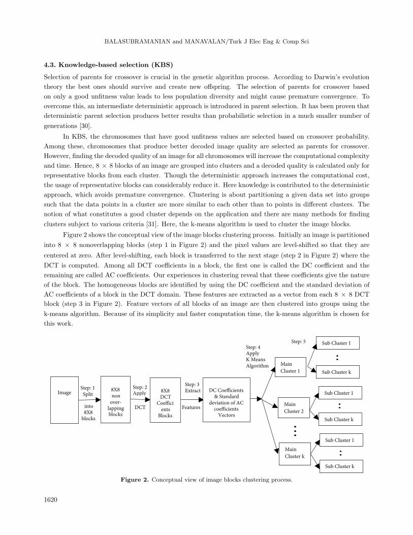
Figure 2 shows the conceptual view of the image blocks clustering process. Initially an image is partitioned
into 8 × 8 nonoverlapping blocks (step 1 in Figure 2) and the pixel values are level-shifted so that they are
centered at zero. After level-shifting, each block is transferred to the next stage (step 2 in Figure 2) where the
DCT is computed. Among all DCT coefficients in a block, the first one is called the DC coefficient and the
remaining are called AC coefficients. Our experiences in clustering reveal that these coefficients give the nature
of the block. The homogeneous blocks are identified by using the DC coefficient and the standard deviation of
AC coefficients of a block in the DCT domain. These features are extracted as a vector from each 8 × 8 DCT
block (step 3 in Figure 2). Feature vectors of all blocks of an image are then clustered into groups using the
k-means algorithm. Because of its simplicity and faster computation time, the k-means algorithm is chosen for
this work.
Step: 5 Step: 4 Apply K Means Algorithm
Features
Step: 3 Extract
into 8X8
blocks
DCT
Step: 2 Apply
Step: 1 Split
Main
Cluster 1
Main
Cluster 2
Main
Cluster k
Image 8X8 non
over- lapping blocks
8X8 DCT
Coe"icients
Blocks
DC Coe"icients
& Standard deviation of AC
coe"icients Vectors
Sub Cluster 1
Sub Cluster k
Sub Cluster k
Sub Cluster 1
Sub Cluster 1
Sub Cluster k
Figure 2. Conceptual view of image blocks clustering process.
1620
BALASUBRAMANIAN and MANAVALAN/Turk J Elec Eng & Comp Sci
Initially image blocks are grouped into main clusters using the DC coefficient (step 4 in Figure 2) and
each main cluster is again grouped into subclusters using the standard deviation of the AC coefficients (step
5 in Figure 2). The novelty of the clustering scheme lies in choosing the initial centroids based on a centroid
initialization algorithm, which is described in Algorithm 3. This algorithm overcomes the drawbacks of choosing
the initial centroids randomly in k-means clustering [32,33]. An image block that is nearest to the centroid of
a cluster is chosen as a representative. Algorithm 4 gives the knowledge-based selection algorithm.
Algorithm 3: Centroid initialization algorithm
Input : Set of N data vectors (data set), K (number of clusters)
Output : Initial cluster centroids
i) Sort the data vectors in ascending order.
ii) Split the ordered vectors into K bins randomly.
iii) Calculate the mode for each bin and consider as initial centroids.
Algorithm 4: Knowledge-based selection algorithm
Input : Cluster-representative blocks and superior chromosomes
Output : Chromosomes for crossover
i) Perform quantization and dequantization for the cluster representatives using superior chromosomes and
calculate peak signal-to-noise ratio (PSNR) value.
ii) Select the chromosomes that give a high PSNR value for each cluster representative.
4.4. Knowledge-based crossover (KBC)
KBC operates on two chromosomes, which are chosen randomly, and swaps the genes between these two
chromosomes in order to generate two offspring. Generally crossover refers to an exploitation operation, which
cannot generate quite different offspring from the parents because it uses only acquired information. Here the
single-point crossover operator is employed and knowledge is used to select the crossover point. A crossover
point is selected randomly between positions 2 and 25 in a chromosome. The position of genes in a chromosome
is shown in Figure 3. The reason for choosing the crossover points in the top left subtable of a chromosome
is because this subtable interacts with lower order DCT coefficients during quantization, which mainly plays
an important role in the quality of a block. Other subtables have less impact on the quality of a block, so
having more randomness in the top left subtable gives more space to search for the optimal solution. If the
crossover point is selected in any other subtable, then crossover produces infeasible solutions and hence wastes
search time. Here knowledge is contributed to exploring new feasible solutions. The knowledge-based crossover
algorithm is given in Algorithm 5.
1621

BALASUBRAMANIAN and MANAVALAN/Turk J Elec Eng & Comp Sci
1 3 4 10 11 21 22 36
2 5 9 12 20 23 35 37
6 8 13 19 24 34 38 49
7 14 18 25 33 39 48 50
15 17 26 32 40 47 51 58
16 27 31 41 46 52 57 59
28 30 42 45 53 56 60 63
29 43 44 54 55 61 62 64
Figure 3. Gene positions in a chromosome.
Algorithm 5: Knowledge-based crossover algorithm
Input : Superior chromosomes
Output : Offspring
i) Make random pairs of parents without repetition of any chromosome.
ii) Choose the crossover point between gene positions 2 and 25 randomly.
iii) Swap the genes between those two chromosomes.
iv) Find duplicates and replace new ones
4.5. Knowledge-based selective mutation (KBSM)
Mutation is an exploration operation that can search new possible solutions by changing the gene values in the
chromosome randomly. Because the exploratory power of mutation is low, it takes more time to get out of local
optima. Therefore, knowledge-based selective mutation is used to quickly escape from local optima.
KBSM is a process of changing the gene values randomly based on their ranks [34]. Initially rank is
assigned for all superior chromosomes according to their unfitness value, i.e. the superior chromosomes from
the crossover pool are sorted and divided into 6 groups where the group with the lowest unfitness values is
considered as rank one (high rank) and the group with high unfitness values is considered as rank six (low
rank). Chromosomes with high rank are assumed to be nearer to global optima and vice versa. Chromosomes
having high rank will have less genetic change and vice versa. This implies that chromosomes with high unfitness
values are changed very much. Here knowledge is incorporated in this operator to select the mutation point and
value. KBSM is done only in three subtables (top left, top right, and bottom left) of the chromosomes based on
their rank. The reason for choosing these subtables for mutation is because the genes in these positions have
an impact on the quality of the 8 × 8 pixel block. The choosing of genes in each subtable is purely random
and mutation values should be in the ranges of corresponding subtables. Hence, knowledge is contributed the
chromosome to escape from local optima quickly. KBSM is performed based on Algorithm 6.
Algorithm 6: Knowledge-based selective mutation algorithm
Input : Superior chromosomes
Output : Offspring
1622
BALASUBRAMANIAN and MANAVALAN/Turk J Elec Eng & Comp Sci
i) All superior chromosomes from the crossover pool are sorted and divided into 6 groups.
ii) The group with the lowest unfitness values is considered as rank one and the group with high unfitness
values is considered as rank six.
If (rank = 1); mutate one gene in top left subtable.
If (rank = 2); mutate two genes in top left subtable.
If (rank = 3); mutate two genes in top left subtable and one gene in the first two columns of top right
subtable.
If (rank = 4); mutate two genes in top left subtable, one gene in the first two columns of top right
subtable, and one gene in the first two columns of bottom left subtable.
If (rank = 5); mutate two genes in top left subtable, two genes in the first two columns of top right
subtable, and one gene in the first two columns of bottom left subtable.
If (rank = 6); mutate two genes in top left subtable, two genes in the first two columns of top right
subtable, and two genes in the first two columns of bottom left subtable.
iii) Find duplicates and replace new ones.
4.6. Procedure
Initially chromosomes are generated randomly based on KBI. Each chromosome in the initial population is
evaluated by the unfitness function. All the chromosomes are sorted according to their unfitness value. Superior
chromosomes are selected based on low unfitness value. Quantization and dequantization are performed for the
obtained image block cluster representatives by using the superior chromosomes and the PSNR values are
calculated. The chromosome that yields a higher PSNR value for each cluster representative is chosen to
perform the KBC operation and the offspring are produced. Each individual offspring is evaluated by the
unfitness function. These offsprings and parents are sorted and superior chromosomes are identified based on
unfitness value. These superior chromosomes are further processed during KBSM and offspring are produced.
Again the unfitness value is evaluated for each individual offspring. The parent and offspring of KBSM are
considered as the current population and sorted based on their unfitness value. The abovementioned procedure
is repeated until the number of generations is satisfied. The chromosome with the lowest unfitness value after
the required number of generations is finished is the optimal chromosome. Figure 4 shows the flow diagram of
the KBGA process.
4.7. Performance measures
The main objective of the proposed KBGA is to achieve better image quality, to enhance search capabilities,
and to guarantee feasible solutions. To analyze the quality of the decompressed image, the following statistical
measures [1] are used.
1623

BALASUBRAMANIAN and MANAVALAN/Turk J Elec Eng & Comp Sci
Start
Generate N Chromosomes based on Knowledge
based Initialization Image Block
Representatives
from each cluster
Calculate Unfitness ; Choose Superior Chromosomes
Yes
No
Perform Quantization & Dequantization using
S uperior Chromosomes on Cluster Representatives
and Find PSNR
Select Chromosomes with high PSNR from each
Cluster as Parents. Make pairs of Parents randomly
Perform Knowledge Based Crossover
Perform Knowledge Based Selective Mutation
Make Parents & Children as Current Population
Calculate Unfitness ; Choose Superior Chromosomes
Make Parents & O"spring as Current Population
Calculate Unfitness ; Choose Superior Chromosomes
No. of
Generations
Completed?
Output Optimal Chromosome
Figure 4. Flowchart of knowledge-based genetic algorithm process.
i) Mean square error (MSE): gives the average of the square of the difference between the original image
and reconstructed image.
MSE =1
xy
x∑i=1
y∑j=1
∥O (i, j)−R(i, j)∥2 (2)
Here, O (i, j) = original image; R (i, j) = reconstructed image.
ii) Peak-signal-to-noise-ratio (PSNR): defined as the ratio of the squared useful signal peak over the mean
square error in decibels.
PSNR = 10log10
(MAX2
O
MSE
)(3)
1624
BALASUBRAMANIAN and MANAVALAN/Turk J Elec Eng & Comp Sci
Here, MAXO= maximum possible pixel value of the image.
To analyze the enhancement of search capability, the following measures [35,36] are used.
iii) Average unfitness value fa(k): gives the average of the best unfitness values obtained within k generations
in n runs.
fa (k) =fb(k)
n(4)
Here, fb(k) = best unfitness values obtained within k generations; n = number of independent runs.
iv) Likelihood of evolution leap Lel(k): gives the probability of average leaps within k generations among n
independent runs. When a solution of one generation is better than the solution of the previous generation,
then it is said to be a leap. Lel(k) at the k th generation is given in Eq. (??).
Lel (k) =l
n(5)
Here, l = average number of leaps within k generations.
To analyze the production of feasible solutions, the following measure is used.
v) Likelihood of optimality Lopt(k): gives the probability of getting optimal solutions within k generations
among n independent runs. Lopt(k) at the k th generation is given in Eq. (??).
Lopt (k) =m
n(6)
Here, m = number of runs that produced optimal solutions within k generations.
5. Performance analysis
Although the CGA is a powerful tool for the generation of the optimum quantization table, more effort is
needed to minimize the number of generations for optimal results. The proposed KBGA uses knowledge-based
operators such as KBI, KBS, KBC, and KBSM to achieve optimal solutions within a few generations. The
proposed KBGA is implemented on a dual core processor of 2.20 GHz each, with 3 GB of RAM. The algorithm
is realized using MATLAB with test images taken from the USC-SIPI image database with different complexity
levels, which is of size 256 × 256 and digitized to 256 gray levels.
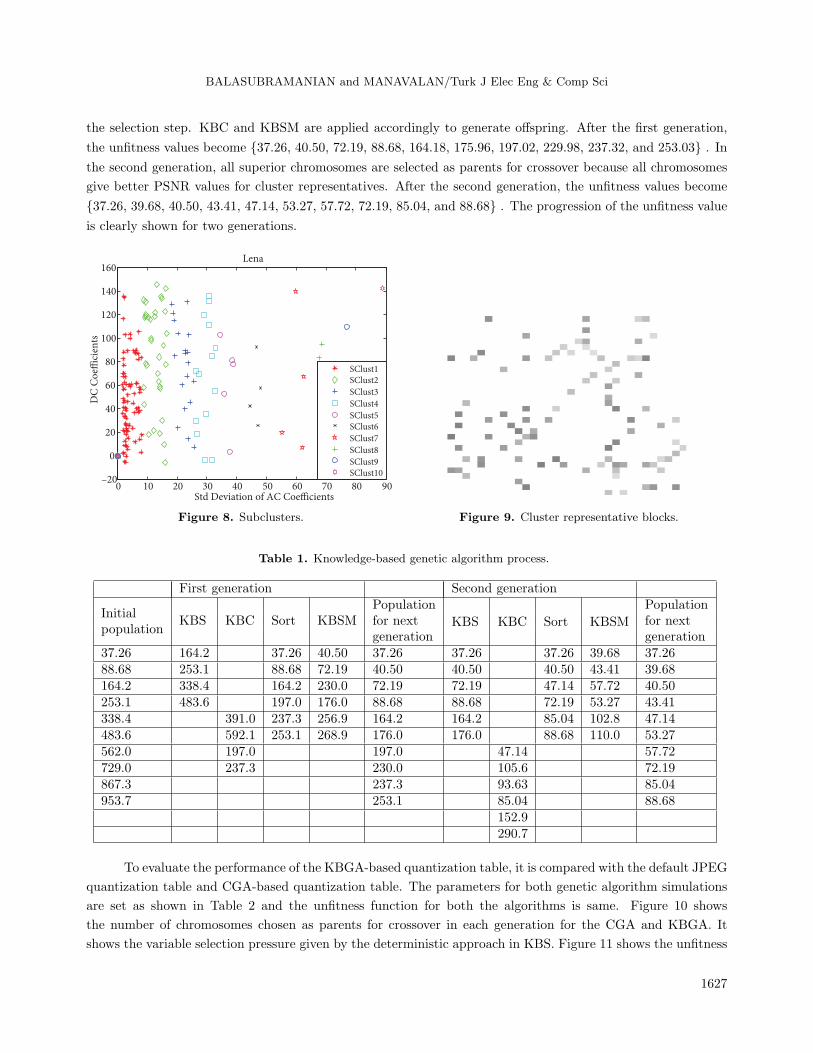
The image block clustering process is incorporated in the selection operator of KBGA to select the
parents for crossover. Experimental results of the image block clustering process are shown for a test image,
Lena, with the target bits per pixel set as 1.0. Figure 5a shows the uncompressed 256 × 256 Lena image.
Figures 6–8 illustrate the result of image block clustering, in which Figure 6 shows all the 1024 DCT blocks
represented by their DC coefficient and standard deviations of AC coefficients. These blocks are clustered into
10 main clusters based on the DC coefficient, as shown in Figure 7. Each main cluster block is then grouped
into 10 subclusters based on the standard deviation of AC coefficients of the corresponding cluster. One of the
subclusters is shown in Figure 8 for a clear view. Different shapes and colors are used to represent different
clusters for better understanding. An empirical analysis based on the brute force method was done for different
numbers of clusters: 50, 75, 100, 125, 150. . . etc. Experimentation with cluster size 100 ≤ cluster size ≥ 200
1625

BALASUBRAMANIAN and MANAVALAN/Turk J Elec Eng & Comp Sci
was carried out in which 100 yielded the same result as 150, 175. . . 200, while the computation time for above
100 was costlier with no fruitful results. Therefore, the total number of clusters was set at 100 (main clusters =
10, subclusters = 10). An image block that is nearest to the centroid of a cluster is chosen as a representative.
Figure 9 shows the representative blocks of the Lena image.
(a) (b) (c) (d) (e)
(f) (g) (h) (i) (j)
Figure 5. Uncompressed test images: (a) Lena, (b) camera man, (c) Barbara, (d) couple, (e) crowd, (f) bridge, (g)
clock, (h) baboon, (i) pattern, (j) montage.
0 10 20 30 40 50 60 70 80 90–1000
–800
–600
–400
–200
0
200
400
600
800
Std Deviation of AC Coe"icients
DC
Co
e"
icie
nts
Lena
DCT Block
0 10 20 30 40 50 60 70 80 90–1000
–800
–600
–400
–200
0
200
400
600
800
Std Deviation of AC Coe"icients
DC
Co
e"
icie
nts
Lena
Clust1
Clust2
Clust3
Clust4
Clust5
Clust6
Clust7
Clust8
Clust9
Clust10
Figure 6. DCT blocks. Figure 7. Main clusters.
Table 1 shows an example for searching for an optimal solution through the proposed KBGA. In this
example, the initial population is 10 chromosomes, crossover probability is 0.6, and mutation probability is 0.015
to 0.093 for ranks 1 to 6, respectively. The unfitness values for the initial 10 chromosomes are {37.26, 88.68,164.18, 253.05, 338.40, 483.62, 562.04, 728.95, 867.33, and 953.67} . Here the first six chromosomes are selected
as superior chromosomes based on crossover probability. Among these six chromosomes, only four are selected
as parents for crossover because only these chromosomes give better PSNR values for cluster representatives.
This satisfies Darwin’s evolution theory and also shows the performance effect of representative block usage in
1626
BALASUBRAMANIAN and MANAVALAN/Turk J Elec Eng & Comp Sci
the selection step. KBC and KBSM are applied accordingly to generate offspring. After the first generation,
the unfitness values become {37.26, 40.50, 72.19, 88.68, 164.18, 175.96, 197.02, 229.98, 237.32, and 253.03} . In
the second generation, all superior chromosomes are selected as parents for crossover because all chromosomes
give better PSNR values for cluster representatives. After the second generation, the unfitness values become
{37.26, 39.68, 40.50, 43.41, 47.14, 53.27, 57.72, 72.19, 85.04, and 88.68} . The progression of the unfitness value
is clearly shown for two generations.
0 10 20 30 40 50 60 70 80 90–20
0
20
40
60
80
100
120
140
160
Std Deviation of AC Coe"icients
DC
Co
e"
icie
nts
Lena
SClust1
SClust2
SClust3
SClust4
SClust5
SClust6
SClust7
SClust8
SClust9
SClust10
Figure 8. Subclusters. Figure 9. Cluster representative blocks.
Table 1. Knowledge-based genetic algorithm process.
First generation Second generation
InitialPopulation
KBS KBC Sort KBSM
Population
populationKBS KBC Sort KBSM for next for next
generation generation37.26 164.2 37.26 40.50 37.26 37.26 37.26 39.68 37.2688.68 253.1 88.68 72.19 40.50 40.50 40.50 43.41 39.68164.2 338.4 164.2 230.0 72.19 72.19 47.14 57.72 40.50253.1 483.6 197.0 176.0 88.68 88.68 72.19 53.27 43.41338.4 391.0 237.3 256.9 164.2 164.2 85.04 102.8 47.14483.6 592.1 253.1 268.9 176.0 176.0 88.68 110.0 53.27562.0 197.0 197.0 47.14 57.72729.0 237.3 230.0 105.6 72.19867.3 237.3 93.63 85.04953.7 253.1 85.04 88.68
152.9290.7
To evaluate the performance of the KBGA-based quantization table, it is compared with the default JPEG
quantization table and CGA-based quantization table. The parameters for both genetic algorithm simulations
are set as shown in Table 2 and the unfitness function for both the algorithms is same. Figure 10 shows
the number of chromosomes chosen as parents for crossover in each generation for the CGA and KBGA. It
shows the variable selection pressure given by the deterministic approach in KBS. Figure 11 shows the unfitness
1627
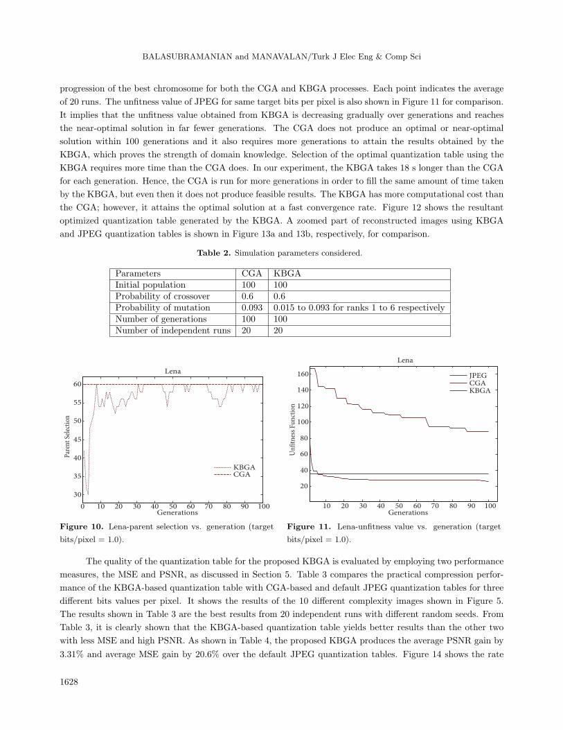
BALASUBRAMANIAN and MANAVALAN/Turk J Elec Eng & Comp Sci
progression of the best chromosome for both the CGA and KBGA processes. Each point indicates the average
of 20 runs. The unfitness value of JPEG for same target bits per pixel is also shown in Figure 11 for comparison.
It implies that the unfitness value obtained from KBGA is decreasing gradually over generations and reaches
the near-optimal solution in far fewer generations. The CGA does not produce an optimal or near-optimal
solution within 100 generations and it also requires more generations to attain the results obtained by the
KBGA, which proves the strength of domain knowledge. Selection of the optimal quantization table using the
KBGA requires more time than the CGA does. In our experiment, the KBGA takes 18 s longer than the CGA
for each generation. Hence, the CGA is run for more generations in order to fill the same amount of time taken
by the KBGA, but even then it does not produce feasible results. The KBGA has more computational cost than
the CGA; however, it attains the optimal solution at a fast convergence rate. Figure 12 shows the resultant
optimized quantization table generated by the KBGA. A zoomed part of reconstructed images using KBGA
and JPEG quantization tables is shown in Figure 13a and 13b, respectively, for comparison.
Table 2. Simulation parameters considered.
Parameters CGA KBGAInitial population 100 100Probability of crossover 0.6 0.6Probability of mutation 0.093 0.015 to 0.093 for ranks 1 to 6 respectivelyNumber of generations 100 100Number of independent runs 20 20
0 10 20 30 40 50 60 70 80 90 100
30
35
40
45
50
55
60
Generations
Pare
nt
Sele
cti
on
Lena
KBGA
CGA
10 20 30 40 50 60 70 80 90 100
20
40
60
80
100
120
140
160
Generations
Un
fitn
ess
Fu
nct
ion
Lena
JPEGCGAKBGA
Figure 10. Lena-parent selection vs. generation (target
bits/pixel = 1.0).
Figure 11. Lena-unfitness value vs. generation (target
bits/pixel = 1.0).
The quality of the quantization table for the proposed KBGA is evaluated by employing two performance
measures, the MSE and PSNR, as discussed in Section 5. Table 3 compares the practical compression perfor-
mance of the KBGA-based quantization table with CGA-based and default JPEG quantization tables for three
different bits values per pixel. It shows the results of the 10 different complexity images shown in Figure 5.
The results shown in Table 3 are the best results from 20 independent runs with different random seeds. From
Table 3, it is clearly shown that the KBGA-based quantization table yields better results than the other two
with less MSE and high PSNR. As shown in Table 4, the proposed KBGA produces the average PSNR gain by
3.31% and average MSE gain by 20.6% over the default JPEG quantization tables. Figure 14 shows the rate
1628

BALASUBRAMANIAN and MANAVALAN/Turk J Elec Eng & Comp Sci
distortion curve for the JPEG, CGA, and KBGA quantization tables. It shows that the KBGA quantization
tables have reduced MSE over the JPEG quantization tables at the same bits per pixel.
32 23 21 19 14 24 31 37
22 21 22 20 16 35 36 33
20 20 18 21 24 34 41 34
20 16 26 23 31 38 48 37
11 23 17 27 41 65 62 46
14 21 33 26 49 62 68 55
29 38 47 52 62 73 72 61
43 55 57 59 67 60 62 59
Figure 12. Optimized quantization table (target bits/pixel = 1.0).
Table 3. Comparison of image quality measures for different target bits/pixels.
Target bits/pixel 0.75 1 1.5
ImageQuantization Bits
MSEPSNR Bits
MSEPSNR Bits
MSEPSNR
table /pixel in dB /pixel in dB /pixel in dB
Lena
JPEG 0.76 51.96 31.01 1.03 34.29 32.81 1.50 19.26 35.31CGA 0.76 83.94 28.92 1.00 88.28 28.71 1.56 81.11 29.07KBGA 0.75 43.27 31.80 1.03 26.36 33.96 1.55 12.35 37.25
Camera Man
JPEG 0.75 66.24 29.95 1.02 44.25 31.71 1.51 22.29 34.68CGA 0.77 116.5 27.50 0.99 105.2 27.94 1.55 119.73 27.38KBGA 0.76 53.24 30.87 1.01 31.29 33.21 1.51 15.50 36.26
Barbara
JPEG 0.77 61.71 30.26 1.01 41.93 31.94 1.50 16.92 35.88CGA 0.77 96.98 28.30 1.04 91.18 28.57 1.51 98.48 28.23KBGA 0.77 48.57 31.30 1.01 28.81 33.57 1.52 12.05 37.35
Clock
JPEG 0.75 24.28 34.31 1.00 14.64 36.51 1.51 7.21 39.58CGA 0.75 79.74 29.15 1.01 61.52 30.27 1.49 59.49 30.41KBGA 0.75 18.66 35.45 1.00 12.06 37.35 1.51 4.72 41.43
Bridge
JPEG 0.75 157.7 26.19 1.03 120.0 27.37 1.61 75.77 29.37CGA 0.76 201.4 25.12 1.05 174.9 25.74 1.65 150.3 26.40KBGA 0.75 144.1 26.58 1.04 103.1 28.03 1.60 61.66 30.27
Couple
JPEG 0.75 49.57 31.21 1.01 34.31 32.81 1.50 19.49 35.27CGA 0.74 71.39 29.63 1.03 84.28 28.91 1.57 87.13 28.76KBGA 0.75 44.36 31.70 1.00 29.55 33.46 1.50 15.01 36.40
Crowd
JPEG 0.76 40.51 32.09 1.01 27.25 33.81 1.52 14.77 36.47CGA 0.74 64.74 30.05 1.03 88.15 28.71 1.53 77.69 29.26KBGA 0.75 37.86 32.38 1.02 24.04 34.36 1.53 11.34 37.62
Baboon
JPEG 0.75 404.2 22.10 1.04 330 22.98 1.54 223.3 24.68CGA 0.74 470.9 21.44 1.02 408.5 22.05 1.49 345.9 22.77KBGA 0.76 368.4 22.50 1.04 282.5 23.66 1.53 183.9 25.52
Pattern
JPEG 0.75 58.63 30.48 1.01 48.10 31.34 1.51 35.91 32.61CGA 0.74 79.43 29.17 0.99 74.87 29.42 1.49 65.98 29.97KBGA 0.75 50.87 31.10 1.01 39.43 32.21 1.51 25.09 34.17
Montage
JPEG 0.75 25.20 34.15 1.00 13.55 36.85 1.50 5.51 40.76CGA 0.76 79.99 29.13 1.01 74.58 29.44 1.53 69.59 29.74KBGA 0.75 17.38 35.76 1.01 10.488 37.96 1.50 2.98 43.42
1629

BALASUBRAMANIAN and MANAVALAN/Turk J Elec Eng & Comp Sci
Table 4. Average MSE and PSNR gain of KBGA-based quantization table over JPEG table.
Bits/pixel Average MSE gain in % Average PSNR gain in %0.75 13.64 2.551.0 20.33 3.021.5 27.83 4.37Average 20.60 3.31
(a) (b)
Figure 13. Reconstructed image by (a) JPEG quantization table and (b) KBGA quantization table.
0.7 0.8 0.9 1 1.1 1.2 1.3 1.4 1.5 1.620
40
60
80
100
120
140
Rate (bits per pixel)
Dis
tort
ion
(M
SE)
Lena
JPEGCGAKBGA
Figure 14. Rate distortion curve of JPEG, CGA, and KBGA quantization tables.
As given in Section 5, performance measures such as average unfitness value fa(k), likelihood of evolution
leap Lel(k), and likelihood of optimality Lopt(k) have been taken into consideration in a comparative study to
show the efficacy of the KBGA. For both the CGA and KBGA, these measures are estimated for 10 different
images by setting target bits per pixels at 0.75, 1.0, and 1.5 in 20 independent runs (totally 10 × 3 × 20 =
600 runs for each algorithm). The results shown in Tables 5–7 are for target bits per pixel set at 1.0. Table 5
1630
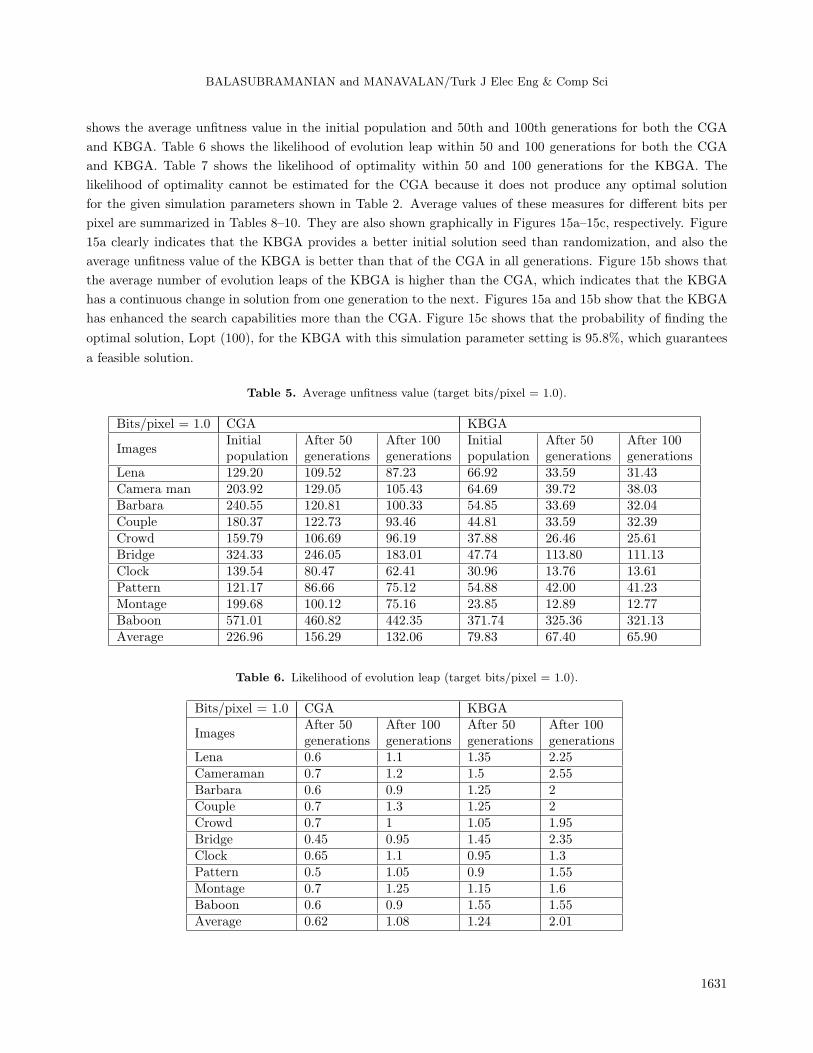
BALASUBRAMANIAN and MANAVALAN/Turk J Elec Eng & Comp Sci
shows the average unfitness value in the initial population and 50th and 100th generations for both the CGA
and KBGA. Table 6 shows the likelihood of evolution leap within 50 and 100 generations for both the CGA
and KBGA. Table 7 shows the likelihood of optimality within 50 and 100 generations for the KBGA. The
likelihood of optimality cannot be estimated for the CGA because it does not produce any optimal solution
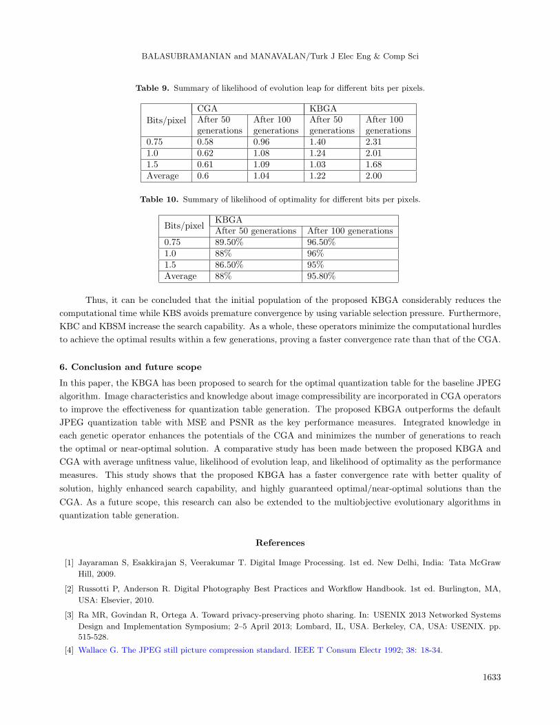
for the given simulation parameters shown in Table 2. Average values of these measures for different bits per
pixel are summarized in Tables 8–10. They are also shown graphically in Figures 15a–15c, respectively. Figure
15a clearly indicates that the KBGA provides a better initial solution seed than randomization, and also the
average unfitness value of the KBGA is better than that of the CGA in all generations. Figure 15b shows that
the average number of evolution leaps of the KBGA is higher than the CGA, which indicates that the KBGA
has a continuous change in solution from one generation to the next. Figures 15a and 15b show that the KBGA
has enhanced the search capabilities more than the CGA. Figure 15c shows that the probability of finding the
optimal solution, Lopt (100), for the KBGA with this simulation parameter setting is 95.8%, which guarantees
a feasible solution.
Table 5. Average unfitness value (target bits/pixel = 1.0).
Bits/pixel = 1.0 CGA KBGA
ImagesInitial After 50 After 100 Initial After 50 After 100population generations generations population generations generations
Lena 129.20 109.52 87.23 66.92 33.59 31.43Camera man 203.92 129.05 105.43 64.69 39.72 38.03Barbara 240.55 120.81 100.33 54.85 33.69 32.04Couple 180.37 122.73 93.46 44.81 33.59 32.39Crowd 159.79 106.69 96.19 37.88 26.46 25.61Bridge 324.33 246.05 183.01 47.74 113.80 111.13Clock 139.54 80.47 62.41 30.96 13.76 13.61Pattern 121.17 86.66 75.12 54.88 42.00 41.23Montage 199.68 100.12 75.16 23.85 12.89 12.77Baboon 571.01 460.82 442.35 371.74 325.36 321.13Average 226.96 156.29 132.06 79.83 67.40 65.90
Table 6. Likelihood of evolution leap (target bits/pixel = 1.0).
Bits/pixel = 1.0 CGA KBGA
ImagesAfter 50 After 100 After 50 After 100generations generations generations generations
Lena 0.6 1.1 1.35 2.25Cameraman 0.7 1.2 1.5 2.55Barbara 0.6 0.9 1.25 2Couple 0.7 1.3 1.25 2Crowd 0.7 1 1.05 1.95Bridge 0.45 0.95 1.45 2.35Clock 0.65 1.1 0.95 1.3Pattern 0.5 1.05 0.9 1.55Montage 0.7 1.25 1.15 1.6Baboon 0.6 0.9 1.55 1.55Average 0.62 1.08 1.24 2.01
1631

BALASUBRAMANIAN and MANAVALAN/Turk J Elec Eng & Comp Sci
Table 7. Likelihood of optimality (target bits/pixel = 1.0).
Bits/pixel = 1.0 KBGAImages After 50 generations After 100 generationsLena 0.85 0.95Cameraman 0.85 0.95Barbara 1.00 1.00Couple 0.85 1.00Crowd 0.85 1.00Bridge 0.85 1.00Clock 0.85 0.90Pattern 1.00 1.00Montage 0.85 0.90Baboon 0.85 0.90Average 8.80 0.96
0 20 40 60 80 1000
0.2
0.4
0.6
0.8
1
1.2
1.4
1.6
1.8
2
Generations(b)
Lel
(k)
CGA
KBGA
0 20 40 60 80 10060
80
100
120
140
160
180
200
220
240
260
Generations(a)
f(k)
CGA
KBGA
0 50 1000
10
20
30
40
50
60
70
80
90
100
Generations(c)
Lo
pt(
k) in
%
KBGA
Figure 15. (a) Average unfitness value vs. generations, (b) likelihood of evolution leap vs. generations, (c) likelihood
of optimality vs. generations for KBGA.
Table 8. Summary of average unfitness value for different bits per pixels.
Bits/pixel
CGA KBGAInitial After 50 After 100 Initial After 50 After 100population generations generations population generations generations
0.75 234.29 155.94 138.08 121.72 90.11 88.901.0 226.96 156.29 132.06 79.83 67.40 65.901.5 274.33 154.18 117.28 53.75 40.13 38.14Average 245.19 155.47 129.14 85.10 65.88 64.31
1632
BALASUBRAMANIAN and MANAVALAN/Turk J Elec Eng & Comp Sci
Table 9. Summary of likelihood of evolution leap for different bits per pixels.
Bits/pixel
CGA KBGAAfter 50 After 100 After 50 After 100generations generations generations generations
0.75 0.58 0.96 1.40 2.311.0 0.62 1.08 1.24 2.011.5 0.61 1.09 1.03 1.68Average 0.6 1.04 1.22 2.00
Table 10. Summary of likelihood of optimality for different bits per pixels.
Bits/pixelKBGAAfter 50 generations After 100 generations
0.75 89.50% 96.50%1.0 88% 96%1.5 86.50% 95%Average 88% 95.80%
Thus, it can be concluded that the initial population of the proposed KBGA considerably reduces the
computational time while KBS avoids premature convergence by using variable selection pressure. Furthermore,
KBC and KBSM increase the search capability. As a whole, these operators minimize the computational hurdles
to achieve the optimal results within a few generations, proving a faster convergence rate than that of the CGA.
6. Conclusion and future scope
In this paper, the KBGA has been proposed to search for the optimal quantization table for the baseline JPEG
algorithm. Image characteristics and knowledge about image compressibility are incorporated in CGA operators
to improve the effectiveness for quantization table generation. The proposed KBGA outperforms the default
JPEG quantization table with MSE and PSNR as the key performance measures. Integrated knowledge in
each genetic operator enhances the potentials of the CGA and minimizes the number of generations to reach
the optimal or near-optimal solution. A comparative study has been made between the proposed KBGA and
CGA with average unfitness value, likelihood of evolution leap, and likelihood of optimality as the performance
measures. This study shows that the proposed KBGA has a faster convergence rate with better quality of
solution, highly enhanced search capability, and highly guaranteed optimal/near-optimal solutions than the
CGA. As a future scope, this research can also be extended to the multiobjective evolutionary algorithms in
quantization table generation.
References
[1] Jayaraman S, Esakkirajan S, Veerakumar T. Digital Image Processing. 1st ed. New Delhi, India: Tata McGraw
Hill, 2009.
[2] Russotti P, Anderson R. Digital Photography Best Practices and Workflow Handbook. 1st ed. Burlington, MA,
USA: Elsevier, 2010.
[3] Ra MR, Govindan R, Ortega A. Toward privacy-preserving photo sharing. In: USENIX 2013 Networked Systems
Design and Implementation Symposium; 2–5 April 2013; Lombard, IL, USA. Berkeley, CA, USA: USENIX. pp.
515-528.
[4] Wallace G. The JPEG still picture compression standard. IEEE T Consum Electr 1992; 38: 18-34.
1633
BALASUBRAMANIAN and MANAVALAN/Turk J Elec Eng & Comp Sci
[5] Lazzerini B, Marcelloni F, Vecchio M. A multi-objective evolutionary approach to image quality/compression ratio
trade-off in JPEG baseline algorithm. Appl Soft Comput 2010; 10: 548-561.
[6] Fung HT, Parker KJ. Design of image adaptive quantization tables for JPEG. J Electron Imaging 1995; 4: 144-150.
[7] Fong WC, Chan SC, Ho KL. Designing JPEG quantization matrix using rate-distortion approach and human visual
system model. In: IEEE 1997 Communications Conference; 8–12 June 1997; Montreal, Canada. New York, NY,
USA: IEEE. pp. 1659-1663.
[8] Long WC, Ching YW, Shiuh ML. Designing JPEG quantization tables based on human visual system. In: IEEE
1999 Image Processing Conference; 24–28 October 1999; Kobe, Japan. New York, NY, USA: IEEE. pp. 376-380.
[9] Viresh R, Livny M. An efficient algorithm for optimizing dct quantization. IEEE T Image Process 2000; 9: 267-270.
[10] Battiato S, Mancuso M, Bosco A, Guarnera M. Psychovisual and statistical optimization of quantization tables
for DCT compression engines. In: IEEE 2001 Image Analysis and Processing Conference; 26–28 September 2001;
Palermo, Italy. New York, NY, USA: IEEE. pp. 602-606.
[11] Zaid AO, Olivier C, Alata O, Marmoiton F. Transform image coding with global thresholding application to baseline
JPEG. In: IEEE 2001 Computer Graphics and Image Processing XIV Brazilian Symposium; 15–18 October 2001;
Florianopolis, Brazil. New York, NY, USA: IEEE. pp. 164-171.
[12] Abu NA, Ernawan F, Suryana N. A generic psycho visual error threshold for the quantization table generation
on jpeg image compression. In: IEEE 2013 Signal Processing and Its Applications Colloquium; 8–10 March 2013;
Kuala Lumpur, Malaysia. New York, NY, USA: IEEE. pp. 39-43.
[13] Jianshu C, Hu C, Eckehard S. On the design of a novel JPEG quantization table for improved feature detection
performance. In: IEEE 2013 Image Processing Conference; 15–18 September 2013; Melbourne, Australia. New York,
NY, USA: IEEE. pp. 1675-1679.
[14] Sherlock B, Nagpal A, Monro D. A model for JPEG quantization. In: IEEE 1994 Speech, Image Processing and
Neural Networks Conference; 13–16 April 1994; Hong Kong, China. New York, NY, USA: IEEE. pp. 176-179.
[15] Jiang Y. JPEG image compression using quantization table optimization based on perceptual image quality assess-
ment. In: IEEE 2011 Signals, Systems and Computers Conference; 6-9 November 2011; Pacific Grove, CA. New
York, NY, USA: IEEE. pp. 225-229.
[16] Wu YG. GA-based DCT quantization table design procedure for medical images. IEE P Vis Image Sign 2004; 151:
353-359.
[17] Costa LF, Veiga ACP. Identification of the best quantization table using genetic algorithms. In: IEEE 2005
Communications, Computers and Signal Processing Pacific Rim Conference; 24–26 August 2005; Victoria, Canada.
New York, NY, USA: IEEE. pp. 570-573.
[18] Bonyadi MR, Dehghani E, Moghaddam ME. A non-uniform image compression using genetic algorithm. In: IEEE
2008 Systems, Signals and Image Processing Conference; 25–28 June 2008; Bratislava, Slovakia. New York, NY,
USA: IEEE. pp. 315-318.
[19] Chen S, An T, Hao L. Discrete cosine transforms image compression based on genetic algorithm. In: IEEE 2009
Information Engineering and Computer Science Conference; 19–20 December 2009; Wuhan, China. New York, NY,
USA: IEEE. pp. 1-3.
[20] Konrad M, Stogner H, Uhl A. Evolutionary optimization of jpeg quantization tables for compressing iris Polar
images in iris recognition systems. In: IEEE 2009 Image and Signal Processing and Analysis Symposium; 16–18
September 2009; Salzburg, Austria. New York, NY, USA: IEEE. pp. 534-539.
[21] Guo SM, Tsai JSH, Chang WH, Wu BH, Guo SJ. Chaos evolutionary programming based jpeg quantization table
generation scheme. In: IEEE 2007 Informatics and Systems Conference; 24–26 March 2007; Cairo, Egypt. New
York, NY, USA: IEEE. pp. 1-7.
[22] Ma H, Zhang Q. Research on cultural-based multi-objective particle swarm optimization in image compression
quality assessment. Optik 2013; 124: 957-961.
1634

BALASUBRAMANIAN and MANAVALAN/Turk J Elec Eng & Comp Sci
[23] Bakirtzis AG, Biskas PN, Zoumas CE, Vasilios P. Optimal power flow by enhanced genetic algorithm. IEEE T
Power Syst 2002; 17: 229-236.
[24] Angelova M, Melo-Pinto P, Pencheva T. Modified simple genetic algorithms improving convergence time for the
purposes of fermentation process parameter identification. Ele Com Eng 2012; 11: 256-267.
[25] Prakash A, Chan FTS, Deshmukh SG. FMS scheduling with knowledge based genetic algorithm approach. Expert
Syst Appl 2011; 38: 3161-3171.
[26] Prakash A, Chan FTS, Liao H, Deshmukh SG. Network optimization in supply chain - a KBGA approach. Decis
Support Syst 2012; 52: 528-538.
[27] Thompson M, Pimentel AD. Exploiting domain knowledge in system-level MPSoC design space exploration. J Syst
Architect 2013; 59: 351-360.
[28] Goldberg DE. Genetic Algorithms in Search, Optimization, and Machine Learning. 1st ed. London, UK: Addison-
Wesley, 1999.
[29] Vivek KG. Theoretical foundations of transform coding. IEEE Signal Proc Mag 2001; 1: 9-21.
[30] Razali NM, Geraghty J. Genetic algorithm performance with different selection strategies in solving TSP. In: WCE
2011 World Congress on Engineering Conference; 6–8 July 2011; London, UK. Hong Kong: IAENG. pp. 1134-1139.
[31] Kanungo T, Mount DM, Netanyahu NS, Piatko CD, Silverman R, Wu AY. An efficient k-means clustering algorithm
analysis and implementation. IEEE T Pattern Anal 2002; 24: 881-892.
[32] Pena JM, Lozano JM, Larranaga P. An empirical comparison of four initialization methods for the k-means
algorithm. Pattern Recogn Lett 1999; 20: 1027-1040.
[33] Celebi ME, Kingravi HA, Vela PA. A comparative study of efficient initialization methods for the k-means clustering
algorithm. Expert Syst Appl 2013; 40: 200-210.
[34] Jung SH. Selective mutation for genetic algorithms. World Academy of Science, Engineering and Technology 2009;
32: 478-481.
[35] Kazuo S. Measures for performance evaluations of genetic algorithms. In: 1997 Information Sciences Conference;
1–5 March 1997; Research Triangle Park, NC, USA. pp. 153-156.
[36] Scrucca L. GA - a package for genetic algorithms in R. J Stat Softw 2013; 4: 1-37.
1635