knight/jones/field instructor guide chapter 1 1...

Knight/Jones/Field Instructor Guide Chapter 1

1-1

1 Concepts of Motion

Recommended class days: 3 (including course introduction)

Introduction and Part I Overview

Each of the seven parts of the textbook opens with an overview and closes with a summary. Each

overview is a pause, before plunging in, to look at the road map of what lies ahead. We rarely

give students any rationale for the directions we take or the choices we make, and this “flying

blind” approach contributes to their difficulty finding any coherence in the course. The

overviews provide at least a brief look at where we’re going, and why.

The Part I Overview introduces the idea of a model. Large numbers of students think that the

purpose of physics is to be exact, to describe reality exactly as it is. They become disturbed and

confused by the cavalier way physicists make what often seem to be outrageous assumptions

about a situation. Part of the art of solving physics problems or analyzing phenomena is choosing

the right model, with the right simplifying assumptions. This is a learned skill, one that students

need help to acquire. You will want to be very explicit throughout the course, but especially in

the first few chapters, with where you are making simplifying assumptions (i.e., using a model of

the situation) and why you are doing so.

Background Information

This is the first of eight chapters on dynamics. The overall goal is to find the connection between

force and motion, which we will do through Newton’s laws. The first four chapters are devoted

to establishing and clarifying just what we mean by the terms force and motion. As noted in the

section on physics education research, students’ ideas about force and motion are quite different

from Newtonian ideas. Students cannot begin to understand Newton’s ideas until they have a

better grasp on what force and motion are.


1-2

Beginning with Chapter 5 we begin to apply Newton’s laws to straight-line, 2D, and

rotational motion. Because of the conceptual difficulties students have with force and motion, in

Chapter 5 we begin by understanding how a single particle responds to forces. Only later in the

chapter do we turn to Newton’s third law and systems of interacting problems. Instructors

charting their course for the first few weeks should look ahead through Chapter 8 to see how all

the pieces will fit together.

Student difficulties with the concept of motion have been well studied (Trowbridge and

McDermott, 1980; Trowbridge and McDermott, 1981; Rosenquist and McDermott, 1987;

McDermott et al., 1987). Difficulties instructors should be aware of include:

• Students don’t readily differentiate between position, velocity, and acceleration. They have a

single, undifferentiated idea of “motion.”

• Students don’t easily recognize change of motion. They tend to see motion holistically, as a

single “event,” and they may find it difficult to compare the motion at two different points in

a trajectory. Thus some students think that a projectile moves at constant speed along its

entire path. This difficulty may stem from never having observed motion very carefully. This

is something you can have them do with classroom demonstrations.

• Position and velocity are sometimes confused. If car B overtakes and passes car A on the

freeway, both traveling in the same direction, some students will say the cars have the same

velocity at the instant when B is alongside A.

• Velocity and acceleration are frequently confused. When asked to draw velocity and

acceleration vectors, students often draw acceleration vectors that mimic the velocity vectors.

At a turning point (end of a pendulum’s swing, top of the motion of a ball tossed straight up,

etc.), nearly all students will insist that the acceleration is zero. This is an especially difficult

belief to change. A significant number of class activities involving turning points are needed

for students to understand this issue.

• Acceleration is associated only with speeding up and slowing down. Very few students

associate acceleration with curvilinear motion. This is not surprising, because a vector

acceleration as we use it in physics is a definition, not a common-sense observation. Some

students may know, from high school physics, that circular motion has a centripetal

acceleration. But this is a memorized fact; almost none can tell you why the acceleration

points to the center.


1-3

• Students identify speeding up with positive values of the acceleration and slowing down with

negative acceleration. This is a difficult idea to change, and for many students it becomes a

serious difficulty when they get to Newton’s second law. They need much practice with

coordinate systems, vectors, and vector components.

These difficulties are compounded by most students’ lack of knowledge of vectors. Formal

definitions, such as a = v / t, are nearly meaningless because most students can’t interpret

v. Velocity and acceleration need to be introduced as operational definitions, and students

need ample opportunities to apply the operations needed to find the displacement d and v.

This is especially true if the definition for a is to make any sense. Much of Chapter 3 is focused

on developing and practicing specific procedures for determining velocity and acceleration

vectors.

A second issue addressed in this chapter is the development of good problem-solving skills.

The section on physics education research discussed the differences between student problem-

solving strategies and expert problem-solving strategies. In particular, students rarely go through

the steps of describing the problem situation through sketches, coordinate systems, and the

identification of known and unknown quantities. Several studies that trained students in these

aspects of problem solving showed significant increases in problem-solving ability (Van

Heuvelen, 1991a; Heller et al., 1992a). Chapter 2 begins the development of a well articulated

problem-solving strategy for mechanics problems, a strategy that won’t be complete until

Chapter 8.

Student Learning Objectives

In covering the material of this chapter, students will

• Understand and use the basic ideas of the particle model.

• Analyze the motion of an object by using motion diagrams as a tool.

• Describe motion in terms of position, displacement, and velocity.

• Express quantities using correct units and significant figures, and to be able to use scientific

notation.

• Gain initial experience with displacement and velocity vectors, and the graphical addition of

vectors.


1-4

Pedagogical Approach

Rather than a traditional Chapter 1 wholey on units and measurement, College Physics: A

Strategic Approach dives right into the consideration of motion. The rationale is that students

should immediately be aware that physics is about phenomena, not the memorization of facts and

formulas. The approach to motion in this chapter—through the use of motion diagrams—is

unconventional but straightforward. We make explicit use of the particle model, the first of many

simplifying models introduced throughout the book. Using the particle model, concepts of

coordinate systems and position, and especially changes in position, are developed. Changes in

position naturally lead to position vectors, introduced at this point only informally as directed

arrows, and then to the concept of velocity. Considerations of acceleration are delayed until

Chapter 2.

In keeping with our emphasis on starting right in with motion, we don’t recommend

explicitly treating units, measurements, and significant figures in class. Instead, have your

students read the appropriate sections in the text, and let them know they’ll be quizzed on this

information. Then, as you work through examples with them over the first few weeks, you can

practice these ideas in context. Some instructors will want to be very careful with significant

figures (as is the book—usually!), while others will be satisfied (as are we) with generally

allowing two/three digit accuracy. The key thing is to get them to understand why they shouldn’t

report 10-digit results from their calculator displays.

Students generally pick up the motion diagram idea quickly, an idea that is reinforced by

having them work out motion diagrams from simple motions demonstrated in class.

Vectors are introduced graphically in the context of displacements, which leads naturally to

the idea of vector addition. You’ll want students to practice doing some basic vector addition

(illustrated in Tactics Box 1.4) before beginning to apply this idea to motion diagrams. Be aware

that some students associate a vector with the specific place it is drawn; they don’t realize that

you can slide a vector to another location. Don’t get complicated for now—Chapter 3 is all about

vectors—just draw a couple of vectors on the board, label them A and B, then ask students to

draw the vector A+ B.

Note: It’s worth explicitly calling students’ attention to the Tactics Boxes. These boxes will help

them develop specific skills.


1-5

In describing motion, students often make very “unconventional” assumptions about the

initial and final conditions. If you ask them to draw a motion diagram of a cannon ball fired from

a cliff, you probably mean for the motion to last from the point where the ball leaves the barrel

until the instant of contact with the ground, and you will draw the diagram showing the motion in

a vertical plane. Students will often include the launching process, the flight through the air, and

various bounces or rolls until the ball stops. Some will probably draw it in a perspective diagram,

and some may even draw it from a bird’s-eye view. You need to explicitly address the

simplifying assumptions we make, especially the issue of where the motion starts and ends. The

larger issue here is learning to separate what’s relevant from what’s irrelevant.

A concern to some instructors is that motion-diagram vectors are labeled v and a, whereas

what we’ve really defined are the average velocity vavg and the average acceleration

aavg. The

motion diagram is an important tool to help students visualize motion, a task that many students

find surprisingly difficult. But for motion diagrams to be useful, they must be simple to use.

Thus motion diagrams purposefully blur the distinction between average and instantaneous

quantities—a distinction that is ultimately important but that is meaningless to students at this

initial stage. There’s no evidence that this lack of distinction hinders students’ ability to

understand and use the proper definitions when they reach kinematics in Chapter 2.

It is important not to start doing any computations in this chapter. The focus is simply on

studying several representations of motion, understanding displacement, speed, and velocity, and

identifying displacement and velocity vectors for different kinds of motion. The “problems” in

the examples and in the homework are for the purpose of learning to describe a problem

statement with a pictorial representation. You should emphasize to students that they are not

being asked to solve the problems at this time. There is a statement to that effect in the

homework, but some students will overlook it and plunge right into half-remembered equations

from high school.

Suggested Lecture Outlines

There is no one “right” way to teach physics. The ideas for using class time in this and

subsequent chapters are meant as suggestions. These ideas present an active-learning approach

that has been successful for the authors and for other instructors. Adopt as much or as little of


1-6

this approach as you need. The most important aspect of using class time effectively is not the

specific activities as much as it is keeping the students actively engaged in the learning process.

DAY 1: Most instructors will spend much of Day 1 on logistical details about the course. It is

important to be clear about how you will be using class time and about your expectations of

students. Let them know that you’re going to start right in by asking them to use the information

in Chapter 1, and that an initial chapter reading before Day 2 is essential. To save time, and

because reading is more efficient than listening, we recommend putting all logistical course

information and a day-by-day schedule on a handout for the students. Then, when reviewing

your expectations, tell them that the reading quiz at the beginning of Day 2 will cover both

Chapter 1 and the handouts!

Although it’s hard to have more than half of Day 1 to really use, this is enough time to

introduce the idea of a motion diagram by asking students to imagine cutting apart the frames of

a movie, stacking them, and projecting them onto a screen. Ask a student to walk steadily across

the front of the room, then show how this gets converted to a motion diagram. Draw stick

figures; don’t use the particle model on Day 1 and don’t introduce position or velocity. Note that

if you ask students to “hold up your movie camera and film the motion,” you’ll see that many

pivot to “track” the student who is walking. You’ll need to remind them to keep the camera fixed

so that the object moves across the frame.

Once the basic idea is clear, have various students demonstrate speeding up, slowing down,

or maybe both. To keep these initial motions as simple as possible, identify some points in the

room (such as the ends of the lecture table) as being the edges of the camera’s field of view. That

way a student can speed up across the field of view, but students “won’t see” and won’t be

distracted by his sudden deceleration before hitting the wall! You might ask a student to speed up

slowly while you count frames—1, 2, 3, . . . Then you can ask students to compare the distance

traveled between frames 1 and 2 to the distance between frames 5 and 6.

Have students draw each motion diagram and then compare it with their neighbor’s (a first-

day introduction to the idea of peer interactions). Then put your version on the board. Students’

initial motion diagrams tend to be unbelievably messy and poorly structured, so you quickly—

even when most students seem to have the right idea—want to demonstrate what a “good”

diagram looks like. Putting your version on the board also gives you the opportunity to clarify

subtle points and to give positive reinforcement. Many students who have it right will be very

unsure about their answer.


1-7

DAY 2: Have students observe various real-world motions carefully, then draw a motion

diagram using the particle model. A large strobe lamp, if available, can help clarify how objects

move. Some good real-world trajectories include

• A ball rolled down an incline, from the moment you release it until just before it reaches the

bottom. (This is a good place for a digression on the “start” and the “end” of the motion.)

• A cart rolled across a table with enough friction that it slows and stops.

• Balls tossed in a high parabolic trajectory so that they visibly slow but don’t stop.

• A ball rolled along the table, up a ramp, and back down.

Ask students to focus on the shape of the trajectory and on how the speed changes, drawing the

particles further apart when the object is moving faster.

Position and displacement. Now you can introduce motion diagrams placed on a coordinate

axis, with times assigned to each particle position. To make things concrete, it can be helpful to

use your local east-west highway as the x-axis. Ask how they might report, via cell phone, their

position on the highway to a friend back at school. Sometimes they might say “I’m passing the

gas station,” but at other times, when far from any landmark, they might report “I’m 2 miles east

of the gas station.” This locution brings out three key aspects of any coordinate system: You

need an origin, from which all positions are measured; your distance from the origin; and on

which side of the origin you’re on. You can then go on to discuss our standard x-axis,

superimposed on the highway, with the origin at the gas station. Point out that we denote

positions by the coordinate x (or y for vertical motion). When the object is to the left of the

origin x is negative, and when it is to the right of the origin x is positive. (We also adopt the

convention that positive values of y increase going up. We recommend against using coordinate

systems where positive y’s are down, even for examples such as a falling ball. Students find this

very confusing.)

Since we’re interested in the motion of objects, we need to be able to describe changes in an

object’s position. Imagine you’re standing at initial position x

i= 3 m, and you walk to final

position x

f= 7 m. Then the change in your position—your displacement—is 4 m. Notice that

this is found by taking (7 m) (3 m). In general, then, the displacement is

x = x

fx

i.

Mention that displacements can be negative, indicating motion to the left.


1-8

Clicker Question: Maria is at position x = 23 m. She then undergoes a displacement

x = 50 m. What is her final position?

A. –27 m

B. –50 m

C. 23 m

D. 73 m

Time. To introduce the time “coordinate,” you can draw a simple motion diagram like this one,

and ask whether it represents a person moving to the left or to the right.

0 1 2 3 4 5x (m)

Of course, you really can’t tell without more information. We need to label the time at each

particle position. You can briefly discuss the idea of “clock readings” and the origin of time (i.e.,

how we assign t = 0). Here’s an example they can work out, which also serves as a lead-in to

the concept of velocity.

Example: Jane walks to the right at a constant rate, moving 3 m in 3 s. At t = 0 s she passes the

x = 1 m mark. Draw her motion diagram from t = 1 s to t = 4 s.

Speed and Velocity. To introduce the ideas of speed and velocity it’s important to connect

what students intuitively know about “moving fast” and “moving slow” to our motion diagrams:

Clicker Question: Two runners jog along a track. The positions are shown at 1 s intervals.

Which runner is moving faster?

0 10 20 30 40 50x (m)

AB

But there’s more to this idea. Try the following:

Clicker Question: Two runners jog along a track. The times at each position are shown.

Which runner is moving faster?

0 10 20 30 40 50

0 2 4 6 8 10

1 3 5 7 90 2 4 6 8 10

x (m)B

A

A. Runner A

B. Runner B

C. Both runners are moving at the same speed.


1-9

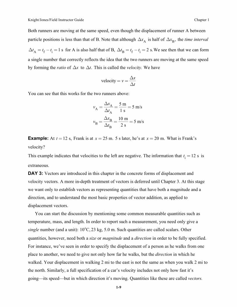
Both runners are moving at the same speed, even though the displacement of runner A between

particle positions is less than that of B. Note that although

xA

is half of

xB

, the time interval

tA

= tf

ti= 1 s for A is also half that of B,

tB

= tf

ti= 2 s.We see then that we can form

a single number that correctly reflects the idea that the two runners are moving at the same speed

by forming the ratio of x to t. This is called the velocity. We have

velocity = v =

x

t

You can see that this works for the two runners above:

vA

=x

A

tA

=5 m

1 s= 5 m/s

vB

=x

B

tB

=10 m

2 s= 5 m/s

Example: At t = 12 s, Frank is at x = 25 m. 5 s later, he’s at x = 20 m. What is Frank’s

velocity?

This example indicates that velocities to the left are negative. The information that ti= 12 s is

extraneous.

DAY 3: Vectors are introduced in this chapter in the concrete forms of displacement and

velocity vectors. A more in-depth treatment of vectors is deferred until Chapter 3. At this stage

we want only to establish vectors as representing quantities that have both a magnitude and a

direction, and to understand the most basic properties of vector addition, as applied to

displacement vectors.

You can start the discussion by mentioning some common measurable quantities such as

temperature, mass, and length. In order to report such a measurement, you need only give a

single number (and a unit): 10°C, 23 kg, 5.0 m. Such quantities are called scalars. Other

quantities, however, need both a size or magnitude and a direction in order to be fully specified.

For instance, we’ve seen in order to specify the displacement of a person as he walks from one

place to another, we need to give not only how far he walks, but the direction in which he

walked. Your displacement in walking 2 mi to the east is not the same as when you walk 2 mi to

the north. Similarly, a full specification of a car’s velocity includes not only how fast it’s

going—its speed—but in which direction it’s moving. Quantities like these are called vectors.


1-10

Discuss our notation for vectors—a symbol with an arrow over it—and stress that it’s crucial to

properly use this notation for all vectors, and not to use it for other, scalar, quantities.

Displacement vectors. Introduce displacement vectors by drawing a motion diagram, and

then drawing the vectors spanning succesive particle positions. Point out that each vector has

both a length (the magnitude of the displacement) and a direction.

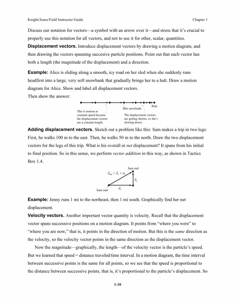
Example: Alice is sliding along a smooth, icy road on her sled when she suddenly runs

headfirst into a large, very soft snowbank that gradually brings her to a halt. Draw a motion

diagram for Alice. Show and label all displacement vectors.

Then show the answer:

This is motion atconstant speed becausethe displacement vectorsare a constant length.

Hits snowbankStop

The displacement vectors are getting shorter, so she’sslowing down.

Adding displacement vectors. Sketch out a problem like this: Sam makes a trip in two legs:

First, he walks 100 m to the east. Then, he walks 50 m to the north. Draw the two displacement

vectors for the legs of this trip. What is his overall or net displacement? It spans from his initial

to final position. So in this sense, we perform vector addition in this way, as shown in Tactics

Box 1.4.

dnet � d1 � d2r r

d1r

d2r

Sam end

Sam start

Example: Jenny runs 1 mi to the northeast, then 1 mi south. Graphically find her net

displacement.

Velocity vectors. Another important vector quantity is velocity. Recall that the displacement

vector spans successive positions on a motion diagram. It points from “where you were” to

“where you are now,” that is, it points in the direction of motion. But this is the same direction as

the velocity, so the velocity vector points in the same direction as the displacement vector.

Now the magnitude—graphically, the length—of the velocity vector is the particle’s speed.

But we learned that speed = distance traveled/time interval. In a motion diagram, the time interval

between successive points is the same for all points, so we see that the speed is proportional to

the distance between successive points, that is, it’s proportional to the particle’s displacement. So


1-11

the length of the velocity vector is proportional to the length of the displacement vector. It’s

simplest to make it the same length as the displacement vector, meaning that you can draw the

velocity vector as also spanning successive particle positions.

Example: Jack throws a ball at a 60° angle, measured from the horizontal. The ball is caught

by Jim. Draw a motion diagram of the ball with velocity vectors.

Other Resources

In addition to the specific suggestions made above in the daily lecture outlines, here are some

other suggestions for questions you could weave into your class time.

Sample Reading Quiz Questions

1. What is the difference between speed and velocity?

a. Speed is an average quantity while velocity is not.

b. Velocity contains information about the direction of motion while speed does not.

c. Speed is measured in mph, while velocity is measured in m/s.

d. The concept of speed applies only to objects that are neither speeding up or slowing

down, while velocity applies to every kind of motion.

e. Speed is used to measure how fast an object is moving in a straight line, while velocity is

used for objects moving along curved paths.

2. The quantity 2.67 103 m/s has how many significant figures?

a. 1

b. 2

c. 3

d. 4

e. 5

3. If Sam walks 100 m to the right, then 200 m to the left, his net displacement vector points

a. to the right.

b. to the left.

c. has zero length.

d. Cannot tell without more information.


1-12

4. Velocity vectors point

a. in the same direction as displacement vectors.

b. in the opposite direction as displacement vectors.

c. perpendicular to displacement vectors.

d. in the same direction as acceleration vectors.

e. Velocity is not represented by a vector.

knight/jones/field instructor guide chapter 1 1...

Documents