kinetic oppp ytimization of speed and efficiency in fast ... · kinetic oppp ytimization of speed...

Kinetic Optimization of Speed and Efficiency p p yin Fast Ultra-High Resolution HPLC

M.M. Dittmann (1) , K. Choikhet (1) , G. Desmet (1)

(1) Agilent Technologies, Waldbronn, Germany(2) Vrije Universeit, Brussels, Belgium

© Agilent Technologies© Agilent Technologies

Introduction

The kinetic plot model (KPM) has been extensively used to investigate performance of columns based on efficiency and permeability mainly onperformance of columns based on efficiency and permeability mainly on isocratic separations.

The first part of this presentation will demonstrate how the model can beThe first part of this presentation will demonstrate how the model can be extended to allow the optimization of gradient separations a a function of column performance and compound retention parameters

In the second part the model was used the investigate the influence of extra column contribution - in particular the influence of connection capillary diameter - on kinetic performance.

© Agilent Technologies

Column Performance Characteristics

S ca tte r P lo t

1 2 0 0

P vs. u curveL ine C ha rt

9 .5

H-u curve

A = 0 4

Column: Agilent SB-C18 RRHD 2.1x50 mm

8 0 0

1 0 0 0

e dr

op [b

ar]

7

7 .5

8

8 .5

9

P [u

m]

A = 0.4B = 5C = 0.08

Φ = 500

2 0 0

4 0 0

6 0 0

Pres

sure

5

5 .5

6

6 .5

HET

P

lin e ar ve lo c ity (c m /s)0 0 .2 0 .4 0 .6 0 .8 1 1 .2 1 .4

0

lin e ar ve lo c ity [m m /s]2 4 6 8 1 0 1 2 1 4

4

4 .5

N (column length, flow rate) Column permeability

Overall column performance


Overall column performance through kinetic plot method

Kinetic Plot Optimization for isocratic elution

Find L* and N* corresponding to a given t0 and P over a large range of t0Find L and N corresponding to a given t0 and Pmax over a large range of t0

2dPΔ0

max* tdP

L p ⋅Φ⋅

⋅Δ=

η )( *0

*** uHLN ⋅=

0

2max*

0 tdP

u p

⋅Φ⋅

⋅Δ=

η

experimental HETP equation


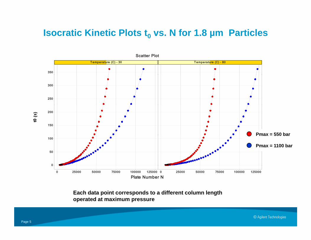
Isocratic Kinetic Plots t0 vs. N for 1.8 µm Particles

Scatter Plot

T e mp e ra ture (C) - 30 T e mp e ra ture (C) - 80

350

250

300

150

200

Pmax = 550 bar

0

50

100Pmax 550 bar

Pmax = 1100 bar

Plate Number N0 25000 50000 75000 100000 125000 0 25000 50000 75000 100000 125000

0

Each data point corresponds to a different column length


operated at maximum pressure

Kinetic Plots for Gradient Separation

In gradient separation the resolution is determined not only by the column plate number but also by the gradient steepness.

Resolution in gradient separation is usually expressed as Peak capacity Pc

Maximum Peak Capacity (Rs= 1) without Maximum Peak Capacity (Rs= 1) with

1 gtP +=

Maximum Peak Capacity (Rs 1) withoutsample imposed limit

1 ., firstrlastr ttP

−+=

Maximum Peak Capacity (Rs 1) withsample imposed limit

)1(0)( et k

Nt

+⋅=σb

ke1

=

σ41cP +

σ41cP +

)1)/'(ln( 00

0 +−⋅++= ttkbbtttt DstartDRN b

ttSb 0⋅Δ⋅= φ

))(( 00 b DstartDR

*P J Schoenmakers et al JCA 149 519 (1978)


gt *P.J. Schoenmakers et al, JCA, 149, 519, (1978)

Variation of Peak Capacity with Gradient Time

Line Chart

193400

Line Chart

260C l l th 100

13.2

15

17

2340

2700

3040

time

s]

S = 6.5ln k’0,1 = 2ln k’0,2 = 6

200

220

240

city

Column length: 100 mmFlow rate: 0.8 ml / min

Sample independent

7.3

9.3

11.2

1300

1640

2000

ΔR

eten

tion

t

4 si

gma

[s

140

160

180

Peak

Cap

ac Sample independent

-0.5

1.4

3.4

5.4

-100

250

600

950Δ80

100

120

Sample dependent

tg (s)

0.5100

0 500 1000 1500 2000 2500 3000

tg (s)0 500 1000 1500 2000 2500 3000 3500

⎥⎤

⎢⎡ +−

⋅=Δ1)/'(ln 00 ttkbtt Dlast


⎥⎥⎦⎢

⎢⎣ +−

=Δ1)/'(

ln0ttkbb

tDfirst

R

Kinetic Plots for Various Gradient Slopes

Scatter Plot


Scatter Plot


Scatter Plot


Scatter Plot


1750

2000

2250

1750

2000

2250

1750

2000

2250

1750

2000

2250

st p

eak

1000

1250

1500

1000

1250

1500

1000

1250

1500

1000

1250

1500

on ti

me

of la

s

250

500

750

250

500

750

250

500

750

250

500

750

Ret

entio

PC column50 100 150 200 50 100 150 200

0

PC column50 100 150 200 50 100 150 200

0

PC column50 100 150 200 50 100 150 200

0

PC column50 100 150 200 50 100 150 200

0

Peak Capacity

t / t = 0 2 t / t = 0 05 t / t = 0 02 t / t = 0 01


t0 / tg = 0.2 t0 / tg = 0.05 t0 / tg = 0.02 t0 / tg = 0.01

Kinetic Plots for fixed Column Length (@ 30 C)Scatter PlotScatter PlotScatter PlotScatter PlotScatter Plot

Pma x syste m (b a r) - 550 Pma x sys te m (b a r) - 1100

4500

5000

L = 30 mm

Scatter Plot


4500

5000

Scatter Plot


4500

5000

Scatter Plot


4500

5000

3500

4000

3500

4000

L = 50 mm3500

4000

L 100

3500

4000

last

pea

k

2000

2500

3000

2000

2500

3000

2000

2500

3000 L = 100 mm

2000

2500

3000

L = 150 mm

tion

time

of l

1000

1500

1000

1500

1000

1500

1000

1500

Ret

ent

Peak capacity (column)0 20 40 60 80 100 120 140 160 0 20 40 60 80 100 120 140 160

0

500


0

500


0

500


0

500

Peak Capacity


Flow Rate Ranges in Fast Gradient LC @ 30 C for 2.1 mm column

Scatter Plot

Pma x syste m (b a r) - 550 Pma x syste m (b a r) - 1100

4500

F < 1 ml/min150 mm

3000

3500

4000F = 1 – 2 ml/min

F > 2 ml/min

ast p

eak

100 mm

150 mm

2000

2500

3000

on ti

me

of la

75 mm

1000

1500

Ret

entio

50 mm

75 mm

75 mm

100 mm


0

500

Peak Capacity

30 mm 30 mm50 mm


Peak capacity (column)Peak Capacity

Flow Rate Ranges in Ultra-Fast Gradient LC @ 80 C for 2.1 mm columns

Scatter Plot

Pma x sys te m (b a r) - 550 Pma x sys te m (b a r) - 1100

225

250

Scatter Plot


225

250

Scatter Plot


225

250

F < 1 ml/min

100 mm100 mm75 mm

175

200

175

200

175

200

F < 1 ml/min

F = 1 – 2 ml/min

F > 2 ml/min

t pea

k 50 mm 75 mm

125

150

125

150

125

150

n tim

e of

last

30 mm

50 mm

50

75

100

50

75

100

50

75

100

Ret

entio

n

30 mm

20 40 60 80 100 20 40 60 80 100

0

25

50

20 40 60 80 100 20 40 60 80 100

0

25

50

20 40 60 80 100 20 40 60 80 100

0

25

50


Peak capacity (column)20 40 60 80 100 20 40 60 80 100



Peak Capacity

Experimental Determination of Peak Capacity

σ41 ., firstrlastr

c

ttP

−+=

t0 marker

First Peak4 σ

Last Peak


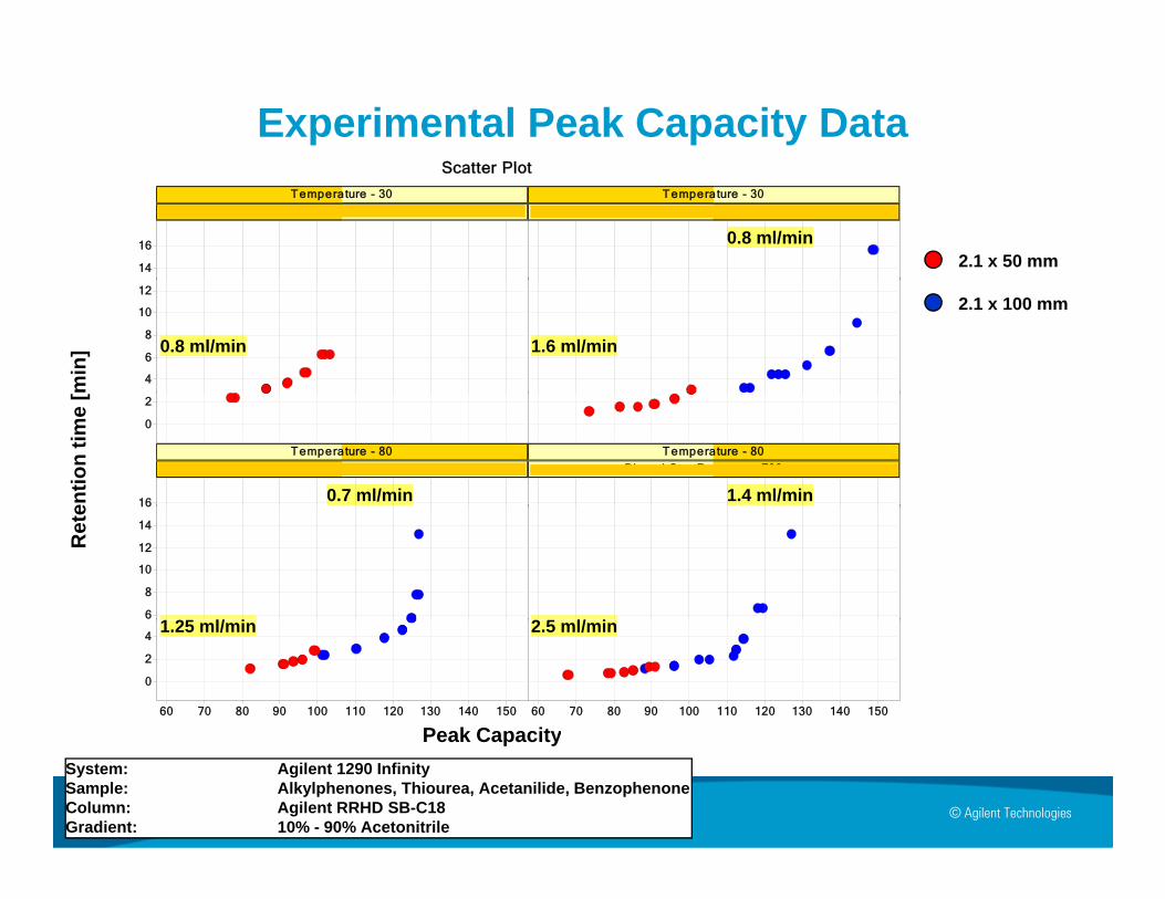
Experimental Peak Capacity DataScatter PlotScatter Plot

Temperature - 30

Binned StartPressure - x = 700

Temperature - 30

Binned StartPressure - 700 < x

14

16 0.8 ml/min2.1 x 50 mm

4

6

8

10

12

0.8 ml/min 1.6 ml/min

min

]

2.1 x 100 mm

Temperature - 80

Binned StartPressure - x = 700

Temperature - 80

Binned StartPressure - 700 < x

16

0

2


entio

n tim

e [

6

8

10

12

14

16

1 25 l/ i 2 5 l/ i

Ret

e

PC60 70 80 90 100 110 120 130 140 150 60 70 80 90 100 110 120 130 140 150

0

2


Peak Capacity


PCPeak CapacitySystem: Agilent 1290 InfinitySample: Alkylphenones, Thiourea, Acetanilide, BenzophenoneColumn: Agilent RRHD SB-C18Gradient: 10% - 90% Acetonitrile

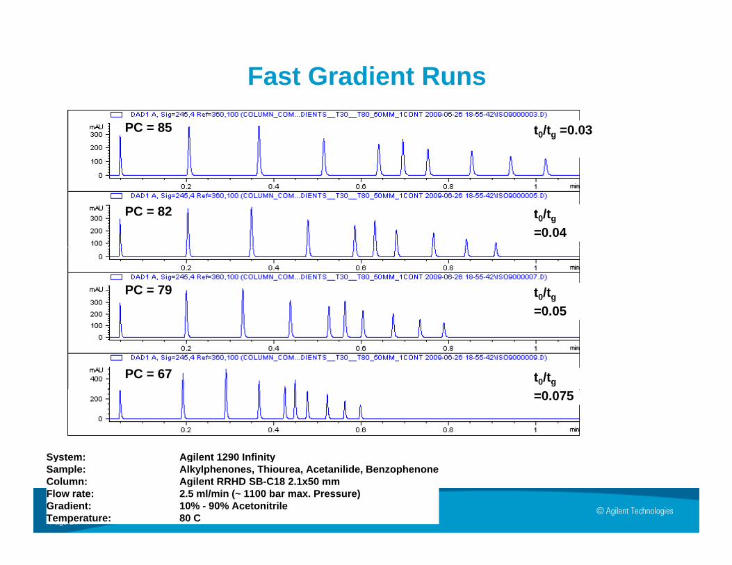
Fast Gradient Runs

t0/tg =0.03PC = 85

t0/tg

=0.04PC = 82

t0/tg

=0.05PC = 79

t0/tgPC = 67

System: Agilent 1290 Infinity

=0.075


y g ySample: Alkylphenones, Thiourea, Acetanilide, BenzophenoneColumn: Agilent RRHD SB-C18 2.1x50 mmFlow rate: 2.5 ml/min (~ 1100 bar max. Pressure)Gradient: 10% - 90% Acetonitrile Temperature: 80 C

Kinetic Plots Including External Band-Broadening

Basic relationships

Pressure drop in a packed column Pressure drop in connection capillaries

0 colcolk d l

LFLuP ⋅⋅=

⋅⋅=Δ

ηη

p p p p(F = volumetric flow rate) (Poiseuille flow)

η8 capLFP

⋅⋅=Δ

02

0 tTcoltmnpackedColu KrK

P⋅⋅

==Δεπ π4

capopenTube r

P =Δ

ηη 8 capcol LFLFP⋅⋅

+⋅⋅

=ΔtFL ⋅= 0insert

πεπ 40

2captTcol

total rKrP +

⋅⋅=Δ

Tcolcol r

FLεπ ⋅

⋅= 2insert

( ) 08

40

2202 =Δ−

⋅

⋅⋅+

⋅⋅

⋅⋅ total

cap

cap

tTcol

PrL

FKr

tFπη

επη Solve for F, determine L


Setup of Low Dispersion System for Determination of Capillary Variance

45 nl injection loop

0.075 x 100 mm PEEK-coated FS capillary

Part to be investigated (column, capillary, HE etc.)

CE-XXCell (13 nl cell volume)

0.050 x 100 mm FS-Capillary


Experimental Determination of Capillary Variance

Line Chart

6

m

CapcapCapillaryV D

FLr⋅

⋅⋅⋅=

24

42

,

πσ Golay equation

5 m

CapcapCapillaryV D

FconstLr⋅

⋅⋅⋅⋅=

24

32.042

,

πσ

empirical equationrimen

tal

3

4

p q

0.170 x 400 mm

σ2[μ

l2 ] e

xpe

1

2 0.120 x 400 mm

Varia

nce

Flow Rate [ml/min]0 0.2 0.4 0.6 0.8 1

0

0.085 x 400 mm


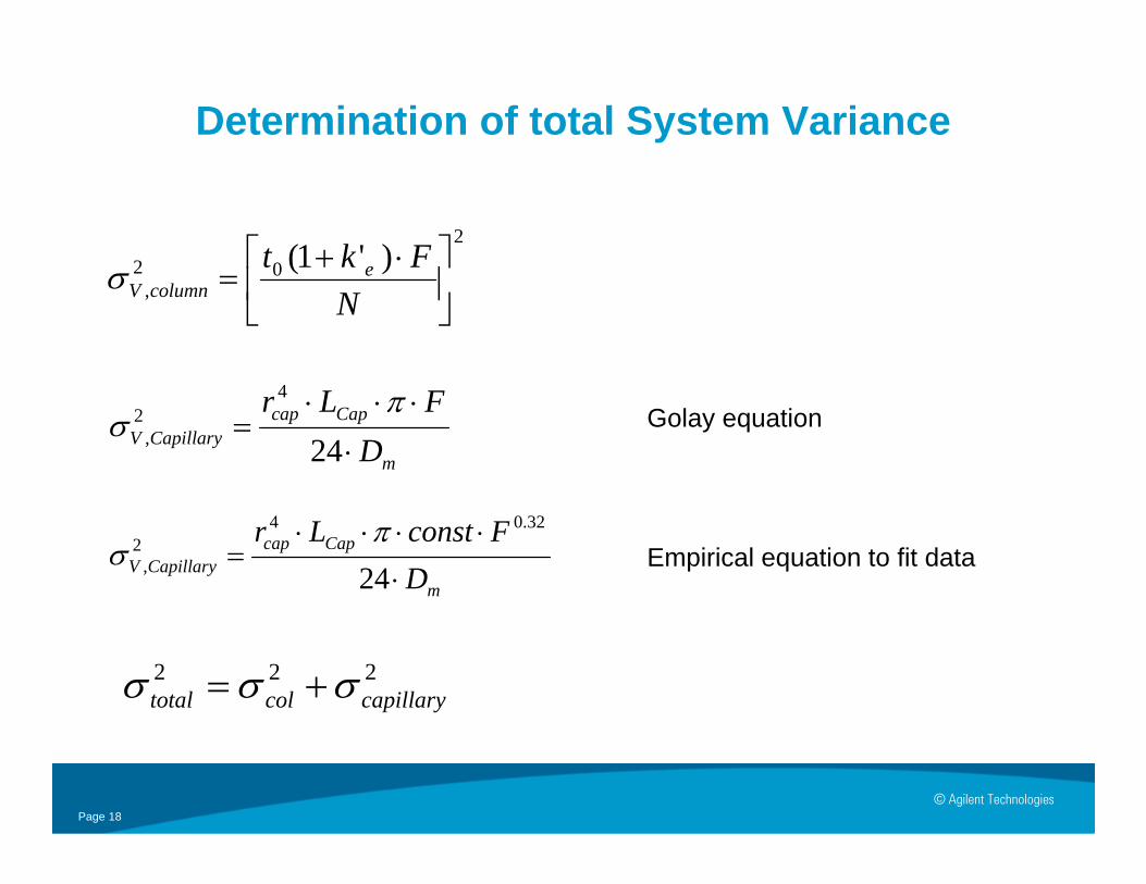
Determination of total System Variance

2

02 )'1(⎥⎤

⎢⎡ ⋅+ Fkt eσ 0

, ⎥⎦

⎢⎣

=N

ecolumnVσ

4

m

CapcapCapillaryV D

FLr⋅

⋅⋅⋅=

24

42

,

πσ Golay equation

m

CapcapCapillaryV D

FconstLr⋅

⋅⋅⋅⋅=

24

32.042

,

πσ Empirical equation to fit data

222capillarycoltotal σσσ +=


Peak Dispersion in System Capillaries

600

700

600

700

0 6 ml/min

300

400

500

sign

al

300

400

500

sign

al

0.3 ml/min

0.4 ml/min

0.6 ml/min

0.3 ml/min

0.4 ml/min

0.6 ml/min

100

200

100

200

0 05 ml/min

0.1 ml/min

0.2 ml/min

0.05 ml/min

0.1 ml/min

0.2 ml/min

00 5 10 15 20

Elution Volume [µl]

00 5 10 15 20

Elution Volume [µl]

0 17 x 105 mm 0 17 x 400 mm

0.05 ml/min

0.17 x 105 mm 0.17 x 400 mm


J.G. Atwood, M.J.A. Golay, JCA, 218, 97(1981)

Kinetic Plots including External Contributions(2.1x30 mm Column) @ 30 °C

Scatter Plot


80

100

t pea

k

60

n tim

e of

las

20

40

Ret

entio

n

Peak capacity (system)20 40 60 80 100 120 20 40 60 80 100 120

0

20

P k C it


Peak capacity (system)Peak Capacity


Scatter Plot


180

140

160

ast p

eak

80

100

120

on ti

me

of la

40

60

Ret

entio

Peak capacity (system)20 40 60 80 100 120 140 20 40 60 80 100 120 140

0

20

Peak Capacity




Scatter Plot


900

700

800

t pea

k

400

500

600

n tim

e of

las

200

300

Ret

entio

n

80 100 120 140 160 180 200 220 240 80 100 120 140 160 180 200 220 240

0

100



Conclusions

The kinetic plot model cannot only be used to compare isocratic f f diff t l b t it t ti ll b d hperformance of different columns but it can potentially be used on a much

broader scale in method development

This method can be employed to optimize separations in gradient mode basedThis method can be employed to optimize separations in gradient mode based on column performance, retention parameters and extra-column contributions.

The kinetic plot model as well as the experimental data suggest that for ultra-fast di t ti th b t f / ti i hi d ll b thgradient separations the best performance / time is achieved well above the

minimum of the van Deemter curve with flow rates in the range of 1 – 3 ml/min at high pressures and temperatures


Acknowledgements

Ken BroekhovenJeroen BillenDeirdre Cabooter

Vrije Universiteit of Brussels


kinetic oppp ytimization of speed and efficiency in fast ... · kinetic oppp ytimization of speed...

Documents