KIER DISCUSSION PAPER SERIES

KYOTO INSTITUTE

OF

ECONOMIC RESEARCH

KYOTO UNIVERSITY

KYOTO, JAPAN

Discussion Paper No.1004

“Implied Ambiguity: Mean-Variance Efficiency and Pricing Errors”

Chiaki Hara and Toshiki Honda

October 2018

Implied Ambiguity:

Mean-Variance Efficiency and Pricing Errors

Chiaki Hara∗ Toshiki Honda†

October 9, 2018

Abstract

We study the optimal portfolio choice problem for an ambiguity-averse in-

vestor having a utility function of the form of Klibanoff, Marinacci, and Mukerji

(2005) and Maccheroni, Marinacci, and Ruffino (2013). We identify necessary

and sufficient conditions for a given portfolio to be optimal for some ambiguity-

averse investor. We also show that the smallest ambiguity aversion coefficient

∗Some results of this paper were included in our previous papers entitled “Asset Demand andAmbiguity Aversio” and “Mutual Fund Theorem for the Ambiguity-Averse Investors and the Op-timality of the Market Portfolio,” which had been circulated since 2013. The research was fundedby “Economic Analysis of Intergenerational Issues: Searching for Further Development,” a Grant-in-Aid for Specially Promoted Research (grant number 22000001) from Japan’s Ministry of Edu-cation, Culture, Sports, Science and Technology; “Equilibrium Analysis on Financial Markets withTransaction costs,” a Grant-in-Aid (A) (grant number 25245046) from the Japan Society for thePromotion of Science; “Capital Asset Pricing Model of Ambiguity-Averse Investors,” from No-mura Fundation; and “Effect of the Change in Trust Act on 2006 on the Efficacy of the Benefi-ciaries’ Decision Making,” from Trust Companies Association of Japan. Hara’s email address ishara.chiaki.7x@kyoto-u.ac.jp.

†The paper is part of the academic project funded by the Grant-in-Aid (grant number 25285097)from Japan’s Ministry of Education, Culture, Sports, Science and Technology. Honda’s email ad-dress is thonda@hub.hit-u.ac.jp. We are both grateful to Robert Anderson, Darrell Duffie, SimonGrant, Youichiro Higashi, Mayumi Horie, Atsushi Kajii, Peter Klibanoff, Nobuo Koida, ChristophKuzmics, Sujoy Mukerji, Frank Riedel, Shuhei Takahashi, Jean-Marc Tallon, Takashi Ui, RyokoWada, Katsuhito Wakai, and participants of our presentations at Kyoto University, HitotsubashiUniversity, Meiji University, Yokohama National University, the 2013 Annual Meeting of the Nip-pon Finance Association, the Swiss-Kyoto Symposium, the 2013 Asian Meeting of the EconometricSociety, the 2014 Annual Meeting of the Korean Association of Financial Engineering, the ZiFResearch Group Workshop on Knightian Uncertainty in Strategic Interactions and Markets, the2015 Annual Meeting of the Asian Finance Association, the 2016 Winter Workshop on OperationsResearch, Finance and Economics, the Fourth and Fifth Asian Quantitative Finance Conferences,Sookmyung Mathematical Finance Conference, and International Conference on Mathematical Fi-nance Conference at CAMP.

1

for the optimality of the given portfolio, which we term the implied ambiguity

of the portfolio, is decreasing with respect to its Sharpe ratio. This relation

can also be expressed in terms of the size of the pricing errors when the as-

set returns are regressed on the return of the portfolio. A numerical analysis

is provided to find the ambiguity aversion implied by the U.S. equity market

data.

JEL Classification Codes: D81, D91, G11, G12.

Keywords: Ambiguity aversion, optimal portfolio, Sharpe ratio, beta, al-

pha, mutual fund theorem.

1 Introduction

Markowitz (1952), Tobin (1958, Section 3.6), Sharpe (1964, Section II), and Lintner

(1965, Sections I to III) laid the foundation of modern portfolio theory. They assumed

that investors care about both the mean and variance of portfolio returns. When,

in addition, a riskless asset is traded and both risky and riskless assets can be sold

short without transaction costs, they established the mutual fund theorem: there is

a common vector of fractions of investment into risky assets that is optimally held

by all investors. The difference in their degrees of risk aversion presents itself as the

difference in the ratio at which their wealth is split between risky assets and riskless

asset. A more risk-averse investor invests less into risky assets, but, of the total

amount invested in risky assets, the fractions over risky assets are the same as those

for a less risk-averse investor.

The portfolio of risky assets held in the optimal fractions is called the tangency

portfolio, which is illustrated in Figure 1. Inside the curve that is convex to the left

are the pairs of means (measured along the vertical axis) and standard deviations

(measured along the horizontal axis) of the returns of all portfolios that consist of

risky assets. The curve represents the smallest variance (or, equivalently, the smallest

standard deviation) of portfolio returns that can be attained while maintaining each

level of the mean. The return on the riskless asset is given as a point on the vertical

axis, because its standard deviation is zero. The line going through the riskelss

return is tangent to the mean-variance efficiency frontier at the return of the tangency

portfolio. It maximizes the slope of the line connecting the riskless return and the

return of any portfolio of risky assets. The slope is equal to the ratio of its expected

2

excess return to standard deviation and known as the Sharpe ratio of the portfolio.

Although the allocation of investment among risky assets should be independent

of investors’ risk aversion according to the mutual fund theorem, such a simple rule

of investment is rarely observed or recommended. Canner, Mankiw, and Weil (1997)

showed that the popular advice on portfolio selection that they surveyed all exhibit

the systematic pattern of increasing investment in the more risky asset class (such as

stocks) and decreasing investment in the less risky one (such as government bonds),

as the investor’s risk aversion decreases. Much more recently, some robo-advisors,

such as Wealthfront, construct a menu of portfolios, each targeted to a particular

level of risk aversion that they infer from the clients’ responses to the questionnaires;

and as the risk aversion decreases, the portfolios put less weights on less risky asset

classes (consisting of, among others, government and corporate bonds in the US) to

more risky ones (consisting of, among others, stocks). These suggested portfolios

contradict the mutual fund theorem. Instead, they should form just a single portfolio

of fixed fractions of investment into various asset classes and advise their clients how

much to invest in it according to their risk aversion.

Albeit involving a process of adding up portfolios and finding an equilibrium, a

more pronounced, and more important, example of contradiction can be found in the

market portfolio in the Captial Asset Pricing Model (CAPM) developed by Sharpe

(1964, Section III) and Lintner (1965, Section IV). If all investors hold scalar multiples

of the tangency portfolio, then the sum of their portfolios is also a scalar multiple

of the tangency portfolio. The sum of their portfolios is, at equilibrium, a scalar

multiple of the market portfolio, in which the investment is allocated in proportion

to the market capitalizations. Thus, the Sharpe ratio of the market portfolio must

be equal to that of the tangency portfolio.

A simple numerical example in Tables 1 and 2, based on the data of the so called

FF6 portfolios in the U.S. equity markets from Ken French’s website, may help us

to see the empirical failure of the mutual fund theorem. The FF6 portfolios are

formed by sorting out traded stocks in terms of the market capitalizations, which is

either Small or Big, and ratio of the book equity to the market equity (B/M), which is

either Low, Neutral, or High, and named the SL, SN, SH, BL, BN, and BH portfolios.

They make up a partially aggregated description of the stock market performance,

less aggregated than the value-weighted portfolio of all available stocks, that allows

us to derive the tangent and market portfolios without suffering from the curse of

3

dimensionality.

The sample means, variances, and covariances of the FF6 portfolios for the period

of August 1926 to December 2017 are reported in Table 1. Table 2 reports the

tangency portfolio based on the data of Table 1 and, as a proxy of the market portfolio,

the value-weighted portfolio of FF6 portfolios, which is computed as the time-series

average of market capitalization weights of FF6 portfoios. The Sharpe ratio of the

tangency portfolio is equal to 0.22, while the Sharpe ratio of the value-weighted

portfolio is equal to 0.13, which is just about sixty percent of the Sharpe ratio of

the tangency portfolio. The value-weighted portfolio, by its definition, holds long all

FF6 portfolios, and invests only two to three percent in each of the SL, SN, and SH

portfolios. The tangency portfolio, on the other hand, exploits the fact that the SN

portfolio has a higher expected return and the smaller variance than the SL portfolio

by containing a large long position in the SN portfolio, which is financed by a large

short position in the SL portfolio.

To reconcile the theory with the reality, we use ambiguity-averse utility functions

initiated by Klibanoff, Marinacci, and Mukerji (2005) (hereafter KMM) and further

explored by Maccheroni, Marinacci, and Ruffino (2013) (hereafter MMR). Let us

emphasize at the outset that we are concerned with the optimal composition of risky

assets, rather than how much of the total wealth is split between the risky assets on

the one hand and the riskless asset on the other. The latter issue is closely related to

the equity premium puzzle of Mehra and Prescott (1985), for example, but we do not

take it up in this paper because, as we will see in Section 2.2, the optimal portfolio in

our model depends neither on the total wealth level nor on the coefficient of relative

ambiguity aversion.

The feature of KMM utility functions that differentiates them from other ambiguity-

averse utility functions, such as those of Gilboa and Schmeidler (1985), is that each

KMM utility function has a probability distribution on a set of distributions of risky

asset returns; and that the aversion to the randomness in the distributions of risky

asset returns and the aversion to the randomness in risky asset returns that would

still remain once the distribution is known are different. The probability distribution

on a set of distributions of risky asset returns represents the perception of ambiguity,

which KMM termed as the second-order belief. They also introduced the ambigu-

ity aversion coefficient, which measures, in the same way as the Arrow and Pratt’

risk aversion coefficient does, how much more averse the investor is to the ambigu-

4

ity in distributions than he is to the remaining randomness after the ambiguity in

distributions is removed.

In this paper, we assume that the second-order belief is concerned with the ex-

pected returns of risky assets; it is a (multivariate) normal distribution; and con-

ditional on the expected returns, the risky asset returns are normally distributed.

We also assume that both the aversion to the ambiguity in distributions and the

aversion to randomness in risky asset returns that still remain after the ambiguity

in distributions is removed are represented by negative exponential utility functions.

The resulting model is an ambiguity-inclusive CARA-normal model; and that the

resulting utility functions are precisely those considered by MMR.

Theorem 2 and Theorem 3 in Section 4 show, first, that a portfolio of risky assets

is optimal for some KMM utility function if and only if its expected excess return

is strictly positive, or, equivalently, its return has a strictly positive Sharpe ratio,

however low it may be. Second, for each portfolio with a strictly positive expected

excess return or Sharpe ratio, they determines the range of the coefficients of absolute

risk aversion with which the given portfolio is optimal. Third, for each coefficient of

risk aversion in this range, they identify the class of pairs of second-order beliefs and

ambiguity aversion coefficients with which the given portfolio is optimal. In particular,

for each coefficient of absolute risk aversion, it gives the smallest ambiguity aversion

coefficient with which the given portfolio is optimal.

Note that the smallest ambiguity aversion coefficient that Theorem 2 and Theorem

3 identify is subject to the choice of the coefficient of absolute risk aversion. By

varying the coefficient of absolute risk aversion, we can find the smallest ambiguity

aversion coefficient with which the given portfolio is optimal. We refer to the smallest

ambiguity aversion coefficient as the implied ambiguity of the portfolio. The most

intriguing result of this paper, Theorem 4, shows that the implied ambiguity is a

strictly decreasing function of the Sharpe ratio. The function is zero where the Sharpe

ratio is equal to the Sharpe ratio of the tangency portfolio, which is optimal for

an ambiguity-neutral investor. As the Sharpe ratio goes down to zero, the implied

ambiguity diverges to infinity, meaning that the portfolio is optimal for an extremely

ambiguity-averse investor.

Let’s illustrate the formula between the Sharpe ratio and the implied ambiguity

in the space of mean and standard deviation of portfolio returns. As can be seen

on Figure 1, the return of the riskless asset is a point on the vertical axis, and the

5

line going through the return of the riskless asset is tangent to the mean-variance

efficiency frontier at the return of the tangency portfolio, as it attains the highest

Sharpe ratio. Thus, if you plot the return of any other portfolio, then the line going

through it and the riskless asset must necessarily be less steep than the tangential

line. This slope determines the implied ambiguity of the portfolio.

We also argue that our result can shed a new light on asset pricing models and

their pricing errors, that is, associated alphas. While we saw the empirical failure of

the mutual fund theorem as a sign of the failure of the CAPM, the statistical test

of the CAPM often takes the form of determining whether there are nonzero alphas,

when the asset returns are regressed on a proxy of the market portfolio. The CAPM

is rejected whenever the hypothesis of zero alphas is rejected; and this has often been

the case in the literature. Gibbons, Ross, and Shanken (1989, Section 3) used the

Hotelling’s T 2 statistic to test the hypothesis of zero alphas. They also showed that

the Sharpe ratio of a portfolio is a decreasing function of the size of alphas when the

asset returns are regressed on the return of the portfolio. Based on this result, we

show in Corollary 1 that the implied ambiguity is an increasing function of the size of

alphas. This corollary is valuable, because it allows us to find the ambiguity aversion

at work in asset markets without relying on other data such as experimental findings

in laboratories.

To establish these results (Theorem 2, Theorem 3, and Theorem 4 in Section 4),

we need to gain a deeper understanding on the optimal portfolios for KMM utility

functions. In our first result (Theorem 1 in Section 3), we show that in our ambiguity-

inclusive CARA-normal setup, the mutual fund theorem no longer holds, and we

characterize the portfolios, which we call the the basis portfolios following Fama

(1996), that constitute the building blocks of ambiguity-averse investors’ optimal

portfolios. The theorem is rich in implications and, among other things, it implies

that once a second-order belief is fixed, the composition of risky assets in the optimal

portfolio depends only on the ambiguity aversion coefficient, and that the coefficient of

absolute risk aversion only affects the ratio at which the total wealth is split between

the risky assets and the riskless asset, just as the standard mutual fund theorem

claims. We also give a sufficient condition under which just one or two basis portfolios

can span the ambiguity-averse investor’s optimal portfolio, regardless of his ambiguity

aversion coefficient, in which case Theorem 1 may legitimately be called a generalized

mutual fund theorem.

6

In order to obtain quantitative implications from our theoretical analysis, we use

U.S. equity market data in Section 6. From the estimates of mean and covariance

of equity returns, we numerically find the implied ambiguity of some representative

portfolios and the associated second-order beliefs. Through the numerical analysis,

we find that the results obtained in our numerical example is robust to the choice

of key parameters such as risk aversion coefficients and the weights in the market

portfolio.

As for the literature, the contributions that are theoretical in nature and most

relevant to this paper have already been mentioned. There is now a growing number

of experimental and empirical papers that dealt with ambiguity aversion.

Ahn, Choi, Gale, and Kariv (2014) and Attanasi, Gollier, Montesano, and Pace

(2014) inferred ambiguity aversion from laboratory experiments on portfolio selection.

Bossaerts, Ghirardato, Guarnaschelli, and Zame (2010) did the same by letting nearly

thirty subjects to trade state-contingent consumptions (Arrow assets) without telling

them the probabilities for some (but not all) states to occur. Ahn, Choi, Gale, and

Kariv (2014) and Bossaerts, Ghirardato, Guarnaschelli, and Zame (2010) concluded

that many subjects are ambiguity-averse, and that they appear to have utility func-

tions of Gilboa and Schmeidler (1989) but not of KMM, because they tend to choose

unambiguous (purely risky) consumption plans, a tendency that is consistent with

utility functions of Gilboa and Schmeidler (1989) but not with those of KMM. Note,

however, that according to Proposition 3 of KMM, the KMM utility functions rep-

resent approximately the same preference relations as the utility functions of Gilboa

and Schmeidler (1989) when the ambiguity aversion coefficient becomes large with-

out bounds. Hence, these experimental results could be interpreted as saying that

the subjects have KMM utility functions with extremely high ambiguity aversion

coefficients.

Collard, Mukerji, Sheppard, and Tallon (2018) found the ambiguity aversion co-

efficients, and the countercyclical nature thereof, using the U.S. equity market data.

Our framework is static while theirs is dynamic, but we deal with multiple stocks while

they deal only with a stock market index (CRSP value-weighted index). In particular,

while we are interested in the optimal composition of stocks for ambiguity-averse in-

vestors, they are more interested in to what extent the equity premium (as measured

by the single stock market index) can be attributed to ambiguity aversion.

Thimme and Volkert (2015) used the consumption and asset market data to es-

7

timate the ambiguity aversion coefficient of the KMM utility function using the gen-

eralized method of moments. Their results and ours are not directly comparable,

because they used a different KMM utility function (which exhibits constant relative,

rather than absolute, risk aversion) and conducted a full econometric analysis (while

our analysis is, so to speak, a quantitative theoretical exercise). Nonetheless, in the

point estimates at which the two papers share the same functional form that repre-

sents ambiguity aversion, and the implied ambiguity of the market portfolio found

in this paper is, in fact, close to the smallest of their point estimate. The two pa-

pers are different in that they fixed the source of ambiguity (which is assumed to

be represented by the riskless return and the price-dividend ratio) at the outset of

their analysis, while we derived it through the minimization of the ambiguity aversion

coefficient that rationalizes the market portfolio.

The rest of this paper is organized as follows. Section 2 sets up the model and

give some preliminary results. Section 3 characterizes optimal portfolios and basis

portfolios. Section 4 provides necessary and sufficient conditions for a portfolio is op-

timal for some ambiguity-averse investor, and derive the relation between the implied

ambiguity and the Sharpe ratio. Section 5 recasts the results of Section 4 to derive

implications on asset pricing. Section 6 obtains the implied ambiguity, second-order

beliefs and associated ambiguity measures, from the U.S. equity market data. Section

7 concludes and suggests directions of future research. All proofs and most lemmas

are given in the appendix.

2 Setup

2.1 Formulation

The setup of this paper is essentially a special case of those of KMM and MMR and

especially close to that of Section 6 of MMR, but we lay it out in a manner that is

more suitable to accommodate the additional parametric assumptions. Let pΩ,F , P q

be a probability space. Let M be a random vector defined on Ω. We will later see

that M is the expected return of assets and represents the ambiguity in the mind of

investors.

For each θ ą 0, define uθ : R Ñ R by letting uθpzq “ ´ expp´θzq for every

z P R. This felicity function exhibits constant absolute risk aversion (CARA) and its

8

coefficient is equal to θ. For each γ ą 0 and each θ ą 0, define a utility function Uγ,θ

over a set of random variables Z on Ω by

Uγ,θpZq “ E“

uγ

`

u´1θ pE ruθpZq |M sq

˘‰

. (1)

The investors who have a utility function Uγ,θ first evaluate the conditional expec-

tation E ruθpZq |M s given M . Then they transform it into the certainty equivalent.

Finally they compute expected utility of those certainty equivalent with respect to

M using the felicity function uγ.

We write η “ γθ ´ 1 and call it the coefficient of relative ambiguity aversion. If

we write φγ,θ “ uγ ˝ u´1θ , then Uγ,θpZq “ E rφγ,θ pE ruθpZq |M sqs. Since

´φ2γ,θpzqp´zq

φ1γ,θpzq

“ η (2)

for every z ă 0, η is equal to the elasticity of the marginal utility from conditional

expectations given M . According to Theorem 2 of KMM, the more concave the

function φγ,θ is, the more ambiguity-averse the investor is, and the larger the value

of η, the more concave the function φγ,θ is.1 We say that the investor is ambiguity-

neutral if γ “ θ, that is, η “ 0. In this case, Uγ,θ is an expected utility function with

CARA coefficient θ. We say that an investor is ambiguity-averse if γ ą θ and η ą 0.

If γ ă θ and η ă 0, then the investor is ambiguity-loving, though we will not pay

much attention to this case.

Assume that two types of assets are traded. The first one is composed of N assets

whose gross returns are represented by an N -variate random vector R defined on Ω.

The second one is the riskless asset whose gross return is deterministic and equal to

Rf P R. We assume also that M is an N -variate random vector, and we take M

as the expected value of R. We further assume that M and R are jointly normally

distributed, and that ErM s “ ErRs and CovrM,Rs “ CovrM,M s. We can thus

write˜

M

R

¸

„ N

˜˜

µ

µ

¸

,

˜

ΣM ΣM

ΣM ΣR

¸¸

. (3)

1This coefficient, however, differs from that of KMM in that they defined the ambiguity aversioncoefficient as ´φ2

γ,θpzqφ1γ,θpzq. We opt for this coefficient of relative ambiguity aversion because it is

constant (independent of z) and still represents the same ranking of concavity as KMM’s definition.

9

This assumption involves no loss of generality.2

Then the conditional return of R given M is normally distributed: R|M „

N`

M,ΣR|M

˘

, where ΣR|M “ ΣR ´ ΣM . Our utility function, thus, embodies the

idea that the investor perceives ambiguity in the expected returns of the risky assets;

once he has come to believe that the expected excess return vector is equal tom P RN ,

he also believes that the asset returns are distributed according to N pm,ΣR|Mq; and

the ambiguity or the model uncertainty is distributed according to N pµ,ΣMq.

Following KMM, we refer to the matrix ΣM as the second-order belief. It rep-

resents the variability of the expected excess returns of the N assets due to model

uncertainty. Of the total covariance matrix ΣR, the second-order belief ΣM is the

covariance matrix of the randomness in asset returns that can be attributed to model

uncertainty, and the remaining covariance matrix, ΣR|M , represents the randomness

in asset returns that still remains even after the model uncertainty is removed. For

the ease of exposition, denote by S N the set of all NˆN symmetric matrices. Denote

by S N`` the set of all symmetric and positive definite N ˆN matrix, and by S N

` the

set of all symmetric and positive semidefinite N ˆN matrix. For every Σ1 P S N and

every Σ2 P S N , we write Σ1 ě Σ2 if Σ1´Σ2 P S N` . The ordering ě on S N

` compares

the sizes of ambiguity perceived by the investor and the smallest second-order belief

is defined with respect to this ordering. We may write Σ1 ď Σ2 when Σ2 ě Σ1, and

0 ď Σ1 to mean Σ1 P ΣN` . Then 0 ď ΣM ď ΣR and 0 ď ΣR|M ď ΣR.

We assume that ΣR P S N`` but not that ΣM P S N

``. The assumption of the

positive definiteness of ΣR means that the N assets are not redundant. By not

imposing the positive definiteness assumption on ΣM , we can accommodates the

situation where there are a fewer common factors underlying model uncertainty of

the expected asset returns.

2It can be shown that even if M did not satisfy this assumption (possibly with a dimensiongreater or smaller than N), some linear transformation of M added by some vector of RN wouldsatisfy this assumption. Indeed, suppose that F is a K-dimensional random vector and

ˆ

FR

˙

„ N

ˆˆ

µF

µR

˙

,

ˆ

ΣF ΣFR

ΣRF ΣR

˙˙

Then there is a D P RKˆN such that ΣRF “ DJΣF . Define M “ DJF ` pµR ´ DJµF q. ThenpM,Rq has the same distribution as assumed in (3).

10

2.2 Portfolio Choice Problem

Denote by px, yq P RN ˆR a portfolio of these N`1 assets, representing the monetary

amounts invested in each of these assets. Once the state is realized, the portfolio pays

out xJR`yRf . Denote the total wealth to be invested in the N `1 assets by W P R.

Let 1 be the vector in RN of which the N coordinates are all equal to one. Then the

budget constraint on the portfolio px, yq P RN ˆ R is 1Jx ` y ď W . The decision

maker’s utility maximization problem is given by

maxpx,yqPRNˆR

Uγ,θpxJR ` yRfq

subject to 1Jx ` y ď W.(4)

Define Vγ,θ : RN ˆ R Ñ R by letting

Vγ,θpx, yq “ µJx ` Rfy ´1

2xJ

`

γΣM ` θΣR|M

˘

x (5)

for every px, yq P RN ˆ R. Since ΣR|M “ ΣR ´ ΣM , this can be rewritten as3

Vγ,θpx, yq “ µJx ` Rfy ´θ

2xJΣRx ´

γ ´ θ

2xJΣMx.

The following lemma shows that Vγ,θ represents the same preference ordering over the

portfolios as Uγ,θ.

Lemma 1 For every px, yq P RN ˆ R, Uγ,θpxJR ` yRfq “ uγ pVγ,θpx, yqq.

If px, yq is a solution to the utility maximization problem (4), then 1Jx` y “ W .

Hence, by Lemma 1, for every px, yq P RN ˆ R, px, yq is a solution to (4) if x is a

solution to

maxxPRN

Vγ,θpx,W ´ 1Jxq (6)

and y “ W ´ 1Jx. The first-order condition gives the solution to the problem (4) is

that

µ ´ Rf1 “ pγΣM ` θΣR|Mqx “ pθΣR ` pγ ´ θqΣMqx “ θ pΣR ` ηΣMqx. (7)

3Thus, it is what MMR calls a robust mean-variance utility function.

11

Since ΣR ` ηΣM P S N``, this is equivalent to

4

x “1

θpΣR ` ηΣMq

´1pµ ´ Rf1q. (8)

There are two things to note in the optimal portfolio (8).5 First, it is independent

of the total wealth W to be invested in the N ` 1 assets. Thus, any increase in

the total wealth does not affect the money amounts x invested in the N assets, but

the money amount W ´ 1Jx invested in the riskless asset increases exactly by the

same amount as the increment in the total wealth. Second, the fractions p1Jxq´1x

depend on the coefficient η of relative ambiguity aversion, but not on the coefficient

θ of absolute risk aversion. For these reasons, we focus on the composition of risky

assets, but not on the allocation of the total wealth between the risky assets and the

riskless asset.

2.3 Measure of ambiguity perception

One of the building blocks of the KMM utility function is the second-order belief

ΣM . Since it represents the variances and covariances of the expected asset returns,

it would be natural to quantify the ambiguity perceived in the return of portfolio

v as its variance vJΣMv, or standard deviation`

vJΣMv˘12

, with respect to ΣM .

There are, however, multiple second-order beliefs that represent an essentially iden-

tical perception of ambiguity. In this subsection, we propose an appropriate measure

of ambiguity perceived in asset and portfolio returns that does not suffer from com-

plications arising from this multiplicity.

Note first that, for any two triples pθ,ΣM , ηq and pθ1,Σ1M , η1q, if θ1 “ θ and there

is a κ ą 0 such that Σ1M “ κΣM and η1 “ κ´1η, then these two triples give rise to the

same optimal portfolio via (8). This fact indicates that the second-order belief ΣM

4The equality (24) of MMR is an equivalent characterization of the optimal portfolio (8).5In our terminology, a portfolio is a vector of money amounts invested in the N assets. It is, thus,

any N -dimensional vector. In contrast, in the terminology of Fama (1996, page 448), for example,a portfolio is a vector of the fractions of money amounts invested the N assets in the sum of themoney amounts invested in these assets. Its coordinates, thus, add up to one. The difference needssome care when, for example, dealing the beta representation of asset returns. However, the signof the expected excess return of x P RN does not depend on which definition to take. Indeed, theexpected excess return of px, yq P RN ˆR is equal to pxJµ`yRfqpxJ1`yq´Rf , but this is equal topxJ1 ` yq´1

`

xJpµ ´ Rf1q˘

, and it has the same sign as xJpµ ´ Rf1q. The Sharpe ratio of portfolio

x, xJpµ ´ Rf1qpxJΣRxq12, is also independent of the choice of definition.

12

and the coefficient η of relative ambiguity aversion are not completely separable, as

Epstein (2010, Section 2.4) pointed out.6 Second, and more specifically to our setting,

the second-order belief ΣM is also not completely separable from the coefficient θ of

absolute risk aversion. That is, for any two triples of pθ,ΣM , ηq and pθ1,Σ1M , η1q, if

there is a τ P R such that Σ1M “ ΣM`τΣR, θ

1 “ p1`τηq´1θ, and η1 “ p1`τηq´1η, then

they give rise to the same optimal portfolio via (8). Thus, while scalar multiplication

of ΣM and addition of a scalar multiplication of ΣR to ΣM can affect the variance

vJΣMv, they can affect the optimal portfolio only in the way that can be offset by

suitably changing the coefficients of risk and ambiguity aversion. Since ambiguity

perception is relevant only if it manifests itself in the optimal portfolio, the second-

order belief ΣM should not directly be used as a measure of ambiguity perception.

We define a measure of ambiguity perception that is independent of scalar multipli-

cation of ΣM and addition of a scalar multiple of ΣR by normalizing the second-order

belief ΣM in the following manner. Define

λpΣMq “ maxvPRN zt0u

vJΣMv

vJΣRv,

λpΣMq “ minvPRN zt0u

vJΣMv

vJΣRv.

Then λpΣMqΣR ď ΣM ď λpΣMqΣR and, thus, λpΣMq “ λpΣMq if and only if ΣM is a

scalar multiple of ΣR. Define the normalized version of the second-order belief by

ΦpΣMq “

$

&

%

0 if ΣM is a scalar multiple of ΣR,1

λpΣMq ´ λpΣMqpΣM ´ λpΣMqΣRq otherwise.

Then λpΦpΣMqq “ 0 and, unless ΣM is a scalar multiple of ΣR, λpΦpΣMqq “ 1.

Thus, 0 ď ΦpΣMq ď ΣR. Two triples pθ,ΣM , ηq and pθ1,Σ1M , η1q give rise to the same

optimal portfolio via (8) regardless of the expected excess returns µ´Rf1 if and only

if θpΣR`ηΣMq “ θ1pΣR`η1Σ1Mq. Since, under some restrictions on the values of η and

η1,7 this is equivalent to ΦpΣMq “ ΦpΣ1Mq, the normalized version of a second-order

6If κ ą 1, then κ´1ΣM ď ΣR. But, if κ ă 1, it need not be true that κ´1ΣM ď ΣR. It is for thisreason, we will see later i the proof of Theorem 2, that there is a lower bound, but no upper bound,on the coefficient of relative ambiguity aversion with which a given portfolio is optimal.

7This restriction is that ´`

λpΣ1M q ´ λpΣ1

M q˘

η1 ă`

λpΣ1M qλpΣM q ´ λpΣM qλpΣ1

M q˘

ηη1 ă`

λpΣM q ´ λpΣM q˘

η. It is satisfied for all η ą 0 and η1 ą 0 if λpΣM q “ λpΣ1M q “ 0.

13

belief represents the class of all second-order beliefs that give rise to the same optimal

portfolio regardless of the expected excess returns.

With the normalized second-order belief, we define the measure of ambiguity per-

ceived in the return of each portfolio v P RN by

Amb pv |ΣMq ”

ˆ

vJΦpΣMqv

vJΣRv

˙12

. (9)

Then, this measure satisfies 0 ď Amb pv |ΣMq ď 1 for every v, Amb pv |ΣMq “ 0 for

some v P RN , and, unless ΣM is a scalar multiple of ΣR, Amb pv |ΣMq “ 1 for some

v P RN . This measure tells us how large the ambiguity perceived in the return of

portfolio v is relative to the total variance of portfolio v.

3 Optimal portfolio for an ambiguity-averse in-

vestor

In this section, we show that the optimal portfolio consists of what we will call basis

(or spanning) portfolios. To state and prove the theorem, we let ΣX P S N`` and

0 ď ΣM ď ΣX and write

Q ” Σ´1R ΣM .

Then define ζ : p´1,8q Ñ RN by letting

ζpηq “ pI ` ηQq´1Σ´1

R pµ ´ Rf1q (10)

for every η P p´1,8q. Then, for every pθ, ηq P R`` ˆ p´1,8q, (8) can be rewritten

as x “ θ´1ζpηq. The function ζ tells us how investor’s portfolio depends on η, while

the total covariance matrix ΣR and the second order belief ΣM are fixed as they are

embedded in the definition of ζ. In the language of KMM on page 1869, therefore, the

following theorem measures the pure effect of introducing greater ambiguity aversion

into a given economic situation.

Theorem 1 (Optimal portfolio in terms of basis portfolios) Suppose that µ´

Rf1 ‰ 0. Then there are a positive integer K and eigenvectors v1, v2, . . . , vK of Q

14

with distinct eigenvalues λ1, λ2, . . . , λK such that, for every η ą ´1,

ζpηq “

Kÿ

k“1

1

1 ` λkηvk. (11)

Theorem 1 shows, first and foremost, that the optimal portfolios are linear com-

binations of eigenvectors of Q, regardless of the coefficient η of relative ambiguity

aversion. Following Fama (1996), we call these eigenvectors basis portfolios. Each

basis portfolio v is chosen so that the covariance of v and each of the N assets with

respect to the second-order belief ΣM is simply a scaled down version of the covariance

with respect to the total covariance matrix ΣR. In fact, let v be a basis portfolio, with

eigenvalue λ. Then ΣRv is the vector of covariances of returns between the N asset

and portfolio v, and ΣMv is the vector of covariances of expected returns between the

N assets and portfolio v. Since Qv “ λv by definition, ΣMv “ λΣRv.

Theorem 1 is particularly useful when the numberK of the basis portfolio is small.

We now give sufficient conditions, in terms of ΣR and ΣM but independent of µ and

Rf , for there to exist at most two distinct mutual funds that cater for all ambiguity-

averse investor. In this case, Theorem 1 can legitimately be called the generalized

mutual fund theorem.

Proposition 1 (One or two basis portfolios) 1. If there is a λ ě 0 such that

λΣR “ ΣM , then there is a v P RN such that, for every η ą ´1,

ζpηq “1

1 ` ληv.

2. If 0 ă rankΣM ă N and there is a λ ą 0 such that rankΣM`rank pλΣR´ΣMq “

N , then there are a vR P KerΣM and a vA P Ker pΣR ´ΣMq such that, for every

η ą ´1,

ζpηq “ vR `1

1 ` ληvA.

3. If 1 “ rankΣM ă N , then there are a λ ą 0, a vR P KerΣM , and a vA P

Ker pΣR ´ ΣMq such that, for every η ą ´1,

ζpηq “ vR `1

1 ` ληvA.

15

Part 1 gives a sufficient condition for a single mutual fund. Part 2 gives a sufficient

condition for two mutual funds. Part 3 is a special case of part 2, which shows that the

condition of part 2 is met whenever there is essentially only one source of ambiguity. In

part 2 and part 3, the subscripts R and A of vR and vA stand for risk and ambiguity.

They do indeed make sense, because the demand for vR does not depend on the

coefficient η of ambiguity aversion, while the demand for vA vanishes as η becomes

large without bounds.

To know more on the basis portfolio in Theorem 1, we consider the following series

of maximization problems:8

maxvPRN zt0u

vJΣR|Mv

vJΣRv. (12)

That is, we look for a portfolio that maximizes the fraction of the unambiguous part of

the variance of the return of the portfolio v. Denote a solution by v1. Next, let n ě 2

and v1, v2, . . . , vn´1 be portfolios, and consider the following maximization problem,

subject to the constraint that the returns of the portfolios must be uncorrelated with

every preceding portfolio vm with m ď n ´ 1:

maxvPRN zt0u

vJΣR|Mv

vJΣRv

s. t. vJmΣRv “ 0 for every m ď n ´ 1.

(13)

We say that a sequence pv1, v2, . . . , vNq of portfolios is a sequence of solutions to the

sequence of problems (12) and (13) if v1, v2, . . . , vN are obtained by iteratively solving

(12) and (13). The next proposition states the relation between basis portfolios and

a sequence of solutions to (12) and (13), and shows properties of basis portfolios.

Proposition 2 (Eigenvalues and eigenvectors of Q) 1. For every sequence

pv1, v2, . . . , vNq of solutions to the sequence of problems (12) and (13) and for

every n, vn is an eigenvector of Q and its corresponding eigenvalue λn is equal

to`

vJnΣMvn

˘

`

vJnΣRvn

˘

.

2. For every sequence pv1, v2, . . . , vNq of eigenvectors of Q, if vJmΣRvn “ 0 whenever

8Similar maximization problems are used by the statistical factor model applying principal com-ponents to the covariance matrix. See Campbell, Lo, and MacKinlay (1997, Section 6.4) for example.Here, in stead of maximizing the return variance, we maximize in (12) the fraction of variance bypure risky part of uncertainty.

16

m ‰ n and the sequence of the corresponding eigenvalues is non-decreasing, then

it is a sequence of solutions to the sequence of problems (13).

3. The eigenvectors of Q that correspond to distinct eigenvalues are orthogonal to

each other with respect to ΣR.

4. All eigenvalues of Q belong to the closed unit interval r0, 1s.

This proposition states that the eigenvectors of Q can be obtained by iteratively

maximizing the fraction of the unambiguous part of the variance of portfolio returns.

The returns of these eigenvector portfolio are independent with each other with re-

spect to the covariance matrix ΣR.

Proposition 2 can be used to give a simpler expression of the measure of ambiguity

perception in (9). It tells us that λpΣMq “ λ1 and λpΣMq “ λN . Thus, for every

v P RN ,

Amb pv |ΣMq “

ˆ

1

λN ´ λ1

ˆ

vJΣMv

vJΣRv´ λ1

˙˙12

.

Moreover, v is an eigenvector of Q that corresponds to its smallest eigenvalue λ1 if

and only if Amb pv |ΣMq “ 0, and v is an eigenvector of Q that corresponds to its

largest eigenvalue λN if and only if Amb pv |ΣMq “ 1.

4 Ambiguity implied by the Sharpe ratio

4.1 Reverse-engineering problem

In section 3, we found the optimal portfolio of a given ambiguity-averse investor. In

this section, we study a reverse-engineering problem, that is, for a given portfolio, we

ask whether there is an ambiguity-averse investor for whom the portfolio is optimal.

The motivation for this study is to fill in the gap between the theory, the mutual

fund theorem, and the reality, the systematic deviation from the theorem at both

individual and aggregate levels. In doing so, we identify an equivalent condition for a

given portfolio to be optimal for some ambiguity-averse investor; show the multiplicity

of such investors in case there is one; characterizing all such investors; and find the

least ambiguity-averse one of all such investors.

In the subsequent analysis, we will take the total covariance matrix ΣR, the mean

vector µ, the riskless asset return Rf , and a portfolio x as given. Then we infer a

17

coefficient θ of absolute risk aversion, a coefficient η of relative ambiguity aversion, and

a second-order belief ΣM for which the portfolio x is optimal. From a mathematical

viewpoint, we solve equation (8) for θ, ΣM , and η, when Rf , µ, ΣR, and x are given.

From a decision-theoretic viewpoint, we show how much of the total covariance matrix

ΣR the investor attributes to ambiguity and to what extent the investor is averse to

risk and ambiguity if the given portfolio x is optimal for him.

4.2 Necessary and sufficient conditions for the optimality of

a portfolio

Suppose that a portfolio x is optimal and (8) holds for an ambiguity-averse investor

who has the coefficient θ of absolute risk aversion, the second-order belief ΣM , and

the coefficient η of relative ambiguity aversion. Theorem 2 derives some inequalities

that bound the values of θ, η, and ΣM . These inequalities are necessary conditions

for the optimality of portfolio x in terms of the ambiguity-averse investor’s attitudes

towards risk, attitudes toward ambiguity, and perception of ambiguity.

Theorem 2 (Necessary conditions of an optimal portfolio) Let ΣR P S N``, µ P

RN , Rf P R, θ ą 0, ΣM P S N` , η ě 0, and x P RN . Suppose that ΣM ď ΣR and (8)

holds. Then

pµ ´ Rf1qJx ą 0. (14)

Define

θ “pµ ´ Rf1qJx

xJΣRx. (15)

Then

θ ă θ. (16)

Define

vθ “1

θΣ´1

R pµ ´ Rf1q ´ x. (17)

18

Suppose that vθ ‰ 0 and define

ΣθM “

1

pvθqJ ΣRvθ

`

ΣRvθ˘ `

ΣRvθ˘J

, (18)

ηθ “

`

vθ˘J

ΣRvθ

xJΣRvθ. (19)

Then

ηΣM ě ηθΣθM , (20)

η ě ηθ. (21)

The first inequality (14) is the most fundamental one. It states that the expected

excess return of portfolio x is strictly positive. Once this condition is met, the second

inequality (16) gives an upper bound θ on the coefficient of absolute risk aversion.

Finally, (20) gives a lower bound ηθΣθM on the second-order belief ΣM multiplied by

the coefficient η of relative ambiguity aversion; and (21) gives a lower bound ηθ on

the coefficient η of relative ambiguity aversion alone. Note that the lower bounds of

(20) and (21) depend on the coefficient θ of absolute risk aversion.

The bounds in Theorem 2 are also sufficient. Theorem 3 proves, indeed, that

the lower bounds in (20) and (21) are attained by some ambiguity-averse investor’s

second-order belief and coefficient of relative ambiguity aversion.

Theorem 3 (Construction of ambiguity) Let ΣR P S N``, µ P RN , Rf P R, and

x P RN . Suppose that (14) holds. Define θ as in (15). Let θ ą 0 and suppose that

(16) holds. Define vθ as in (17) and suppose that vθ ‰ 0. Define ΣθM , and ηθ as in

(18) and (19). Then 0 ď ΣθM ď ΣR, η

θ ą 0, and

x “1

θ

`

ΣR ` ηθΣθM

˘´1pµ ´ Rf1q. (22)

Theorem 3 shows that ΣθM can be the second-order belief of some ambiguity-

averse investor, because it is positive semidefinite and at most ΣR; ηθ can be the

coefficient of relative ambiguity aversion of some ambiguity-averse investor because

it is strictly positive; and the portfolio x is optimal for the investor with ΣθM and ηθ,

because (22) holds. Theorem 3 implies that the last two inequalities, (20) and (21),

of Theorem 2 constitute a sufficient condition for the portfolio x to be optimal for

19

some ambiguity-averse investor whose coefficient of absolute risk aversion is equal to

θ.

It is illustrative to look at vθ in (17) and ΣθM in (18) of Theorem 2 through the

results of the preceding sections. We see that vθ is defined to fill in the gap between

a scalar multiple of the tangency portfolio and a given portfolio x. The second-order

belief ΣθM is defined so that the variance of any portfolio v with respect to Σθ

M is a

function of its covariance with vθ, because

vJΣθMv “

`

vJΣRvθ˘2

pvθqJΣRvθ.

The corresponding matrix Q defined in Section 2, Σ´1R Σθ

M , has rank 1 and a unique

strictly positive eigenvalue 1. Part 3 of Proposition 1 is therefore applicable to ΣθM ,

with vA equal to a scalar multiple of vθ and λ equal to 1. Hence, for each portfolio

v P RN ,

Amb pv |ΣθMq “

|pvθqJΣRv|

ppvθqJΣRvθq12pvJΣRvq12. (23)

Thus, the measure of ambiguity perceived in the return of v is equal to the absolute

value of the correlation coefficient between the return on the portfolio v and the return

on the portfolio vθ.

4.3 Implied ambiguity and Sharpe ratio

According to Theorem 3, the coefficient ηθ of relative ambiguity aversion is the small-

est one with which x is optimal, given a coefficient θ of absolute risk aversion. In this

subsection, we consider the problem of minimizing the coefficient ηθ of relative am-

biguity aversion by varying θ. Theorem 4 solves this problem and finds the smallest

coefficient of relative ambiguity aversion coefficients that is independent of the choice

of θ. The coefficient, therefore, represents the smallest deviation from ambiguity-

neutral mean-variance utility functions that is necessary for the given portfolio to be

optimal.

We should add a caveat to this exercise. We minimize the coefficient ηθ of relative

ambiguity aversion, but we do not really find the least ambiguity-averse investors,

in the sense of KMM, for whom the given portfolio is optimal. Theorem 2 of KMM

showed that an investor is more ambiguity-averse than another if and only if the

20

function φγ,θ is more concave for the first one than for the second, but the theorem

is valid only when the two investors share the same risk attitudes. More specifically,

suppose that the smallest coefficients ηθ and ηθ1

of relative ambiguity aversion, corre-

sponding to two different coefficients, θ and θ1, of absolute risk aversion, are defined

as in Theorem 2 from a portfolio x. We can say that an investor with utility function

Up1`ηqθ,θ is more ambiguity-averse than the investor with the utility function Up1`ηθqθ,θ

in the sense of KMM, whenever η ą ηθ. But, even when ηθ1

ą ηθ, we cannot say

that the investor with the utility function Up1`ηθ1qθ1,θ1 is more ambiguity-averse than

the investor with the utility function Up1`ηθqθ,θ in the sense of KMM, because θ ‰ θ1.

Nonetheless, we consider the problem of minimizing ηθ by varying θ because, as our

Theorem 1 shows, the composition of the optimal portfolio depends on the coeffi-

cient η of relative ambiguity aversion and but not on the coefficient θ of absolute risk

aversion.

As it turns out, the Sharpe ratio of the optimal portfolio is closely related to the

minimized coefficients of relative ambiguity aversion by varying θ. Formally, define

Sr : RNzt0u Ñ R by

Sr pxq “pµ ´ Rf1qJx

pxJΣRxq12.

The Sharpe ratio of a portfolio is the expected excess return that the portfolio can

attain per unit of standard deviation of its return. It is often considered as a measure

of investment efficiency of the portfolio. The function Sr is homogeneous of degree

zero and maximized at every scalar multiple of the tangency portfolio, say, x ”

Σ´1R pµ ´ Rf1q. The maximized value Sr pxq is equal to

`

pµ ´ Rf1qJΣ´1R pµ ´ Rf1q

˘12.

We thus call the ratio Sr pxq Sr pxq as the normalized Sharpe ratio of portfolio x,

which lies on r´1, 1s. The following theorem gives the relation between the normalized

Sharpe ratio and the minimized coefficients of relative ambiguity aversion by varying

θ.

Theorem 4 (Implied ambiguity) Let ΣR P S N``, µ P RN , Rf P R, and x P RN .

Suppose that (14) holds. Define θ be as in (15). Let θ ą 0 and suppose that (16)

holds. Define ηθ as in (19). Then, as a function of θ defined on p0, θq, ηθ is minimized

21

when θ is equal to

θ˚ ”θ

1 `

˜

1 ´

ˆ

Sr pxq

Sr pxq

˙2¸12

(24)

and the minimized value is equal to

ηθ˚

“

2

˜

1 ´

ˆ

Sr pxq

Sr pxq

˙2¸12

1 ´

˜

1 ´

ˆ

Sr pxq

Sr pxq

˙2¸12

. (25)

Theorem 4 implies that there is a one-to-one correspondence between the normal-

ized Sharpe ratio of a portfolio x and the smallest coefficient of relative ambiguity

aversion with which x is optimal. There is also a one-to-one correspondence between

the normalized Sharpe ratio and the coefficient of absolute risk aversion that attains

the smallest coefficient of relative ambiguity aversion. As the normalized Sharpe ra-

tio decreases from one to zero, the smallest coefficient of relative ambiguity aversion

increases strictly from 0 to 8, and the coefficient of absolute risk aversion decreases

strictly from θ to θ2. We refer to the smallest coefficient ηθ˚

of relative ambiguity

aversion as the implied ambiguity of the portfolio x. As the square-root

˜

1 ´

ˆ

Sr pxq

Sr pxq

˙2¸12

(26)

represents the shortfall of the Sharpe ratio of the return of the portfolio x from the

highest Sharpe ratio, attainable by the tangency portfolio x,9 (25) shows that the

implied ambiguity is an increasing function of the shortfall.

As we mentioned in Footnote 6 in Section 2.3, if a portfolio x is optimal for an

investor with a coefficient η of relative ambiguity aversion, then it is also optimal for

an investor with a coefficient of relative ambiguity aversion that is greater than η.

Thus, a portfolio with a positive expected excess return is optimal for some investor

9The square-root (26) can be shown to be equal to minθpvθqJΣRvθ divided by xJΣRx, where vθ

is defined by (17). As the division is for normalization, it measures the deviation of the portfolio xfrom the scalar multiples of the tangency portfolio in terms of the variances of the returns.

22

with a coefficient η of relative ambiguity aversion if and only if

η ě

2

˜

1 ´

ˆ

Sr pxq

Sr pxq

˙2¸12

1 ´

˜

1 ´

ˆ

Sr pxq

Sr pxq

˙2¸12

.

This is perhaps the easiest-to-grasp relation between the normalized Sharpe ratio and

the coefficient of relative ambiguity aversion.

When choosing among the pθ,ΣθM , ηθq’s in Theorem 2, minimizing ηθ is not the

only “right” criterion. In closing this section, we mention that it is possible to min-

imize, instead, the largest eigenvalue (which is the only strictly positive eigenvalue)

of the aversion-weighted second-order belief ηθΣθM by varying θ. This objective func-

tion may be considered as more appropriate, because, as mentioned in Subsection

2.3, the optimal portfolio depends on ηθΣθM , but not separately on ηθ and Σθ

M . This

minimization can also be solved by Lemma 4 in the appendix.10

5 Ambiguity implied by the pricing errors

In Section 4, we related the shortfall of the Sharpe ratio of a given portfolio to

the implied ambiguity. Note here that the first-order condition (7) for the optimal

portfolio also gives the pricing portfolio (the portfolio whose return replicates the

state price density) of the state price beta model in the sense of Duffie (2001, Section

F of Chapter 1). But the given portfolio x itself is, in general, not the pricing portfolio

of the model because the first-order condition involves ambiguity aversion. In other

words, if we regress the excess returns of the asset on the return of the given portfolio

x, then we would end up with nonzero pricing errors, known as the alphas. In this

section, we relate the size of these pricing errors to the implied ambiguity, and argue

that the relation can be used to assess whether a particular coefficient of relative

ambiguity aversion may appropriately be used for asset pricing models.

Denote the vector of alphas of the given portfolio x by αpxq, then

αpxq ” pµ ´ Rf1q ´pµ ´ Rf1qJx

xJΣRxΣRx. (27)

10Take S “ Σ2 in the lemma.

23

If x satisfies the first-order condition (7), then, by letting Q “ Σ´1R ΣM and multiplying

px ` ηQxqJ from left to both sides of (7), we obtain αpx ` ηQxq “ 0. That is, the

state price beta model is valid when the pricing portfolio is x ` ηQx.

In general, αpxq ‰ 0. In order to quantify the size of this N -dimensional vector,

we use, among other candidates, the norm

`

αpxqJΣ´1R αpxq

˘12. (28)

The choice of the positive definite matrix Σ´1R is appropriate on several statistical and

econometric grounds. First and foremost, the inverse gives the Wald test statistic of

the null hypothesis that the alphas are all zero.11 Shanken (1987) used the inverse

of the covariance matrix of the regression residuals, but the two norms based on

the two different covariance matrices can be shown to be equal by using generalized

inverses. Gibbons, Ross, and Shanken (1989) used the Hotelling’s T 2 statistic, which

is an increasing function of our norm of alphas, to test the null hypothesis that the

alphas are all zero. Hansen and Jagannathan (1997) evaluated the performance of

alternative asset pricing models based on the size of errors in the predicted asset prices

using the inverse of the matrix of the non-central second moments, rather than the

covariance matrix, of asset returns. The difference is, however, inessential, because

we look into the expected excess returns of risky assets under the assumption that

the riskless asset is correctly priced regardless of the choice of second-order beliefs

and coefficients of relative ambiguity aversion.

Let x be a portfolio of zero expected excess return, that is, pµ´Rf1qJx “ 0.12 Then

the norm (28) is maximized when x “ x, the maximized norm`

αpxqJΣ´1R αpxq

˘12

is equal to`

pµ ´ Rf1qJΣ´1R pµ ´ Rf1q

˘12, and the Sharpe ratio Sr pxq is equal to 0.

The norm (28) is minimized when x “ x, the minimized norm`

αpxqJΣ´1R αpxq

˘12

is equal to 0, and the Sharpe ratio Sr pxq is equal to`

pµ ´ Rf1qJΣ´1R pµ ´ Rf1q

˘12.

More generally, the following relation holds between the Sharpe ratio of a portfolio

and the norm of alphas when it is taken as the single pricing factor. It is equivalent

to equality (7) and (23) of Gibbons, Ross, and Shanken (1989, Section 3) and can be

proved via a straightforward calculation.

11Campbell, Lo, and MacKinlay (1997, Section 5.3) gives an extensive account on this point.12Since pµ ´ Rf1qJx “

`

Σ´1R pµ ´ Rf1q

˘JΣRx, x is a zero-beta portfolio against the tangency

portfolio.

24

Lemma 2 (Gibbons, Ross, Shanken (1989)) For every x P RNzt0u,

pSr pxqq2

` αpxqJΣ´1R αpxq “ pµ ´ Rf1qJΣ´1

R pµ ´ Rf1q.

The lemma states that the squared Sharpe ratio of a portfolio and the squared

norm of alphas of the N assets, when the beta relation is taken with respect to the

portfolio, add up to the squared highest Sharpe ratio attainable by the tangency

portfolios. The equality can be rewritten as

ˆ

αpxqJΣ´1R αpxq

αpxqJΣ´1R αpxq

˙12

“

˜

1 ´

ˆ

Sr pxq

Sr pxq

˙2¸12

. (29)

Recall that in Section 4, we saw that the right-hand side, which is the same as

(26), represents the shortfall of the Shape ratio of the return of the portfolio x from

the highest Sharpe ratio, attainable by the tangency portfolio x. We see here that

the normalized norm of alphas,`

αpxqJΣ´1R αpxqαpxqJΣ´1

R αpxq˘12

, is equal to the

shortfall of the Sharpe ratio.

The following corollary of Theorem 4 can be immediately obtained from Lemma

2. It allows us to relate the implied ambiguity with the alphas of the asset returns.

Corollary 1 Let ΣR P S N``, µ P RN , Rf P R, and x P RNzt0u. Suppose that (14)

holds. Define θ be as in (15). Let θ ą 0 and suppose that (16) holds. Define ηθ as in

(19) and θ˚ as in (24). Then

ηθ˚

“

2

ˆ

αpxqJΣ´1R αpxq

αpxqJΣ´1R αpxq

˙12

1 ´

ˆ

αpxqJΣ´1R αpxq

αpxqJΣ´1R αpxq

˙12.

We now argue that Corollary 1 can also enable us to gain some idea on reasonable

coefficients of relative ambiguity aversion. To see how this can be done, recall that

the state price beta model is valid if the ambiguity-induced term ηΣMx is added

to the given portfolio x. Suppose, then, that the given portfolio x is the market

portfolio and that we have somehow come to believe that the representative investor,

who holds the market portfolio by definition, has a coefficient of relative ambiguity

25

aversion equal to 8.13 Unlike the case of coefficient of relative risk aversion, on which

there is a vast literature ever since Mehra and Prescott (1985) raised the equity

premium puzzle, we do not really know whether this coefficient is reasonable. Yet,

we know that the state price beta model has zero alphas if its pricing factor is x `

ηQx, rather than x itself. Since 8 “ p2 ˆ 0.8qp1 ´ 0.8q, Corollary 1 implies that

the unexplained 80% of the expected excess returns with pricing portfolio x can be

removed by assuming the coefficient of relative ambiguity aversion equal to 8. Judging

from the asset pricing literature, a typical opinion in the profession would probably

be that such a high proportion of expected excess returns should not be attributed

to ambiguity aversion alone: rather, market incompleteness, transaction costs, and

other impediments to efficient risk sharing should contribute to the unexplained 80%.

In this sense, the coefficient of relative ambiguity aversion being equal to 8 would

be deemed unreasonably high. The lesson from this exercise is that by combining

with our general understanding on asset pricing, we can use Corollary 1 to assess if a

coefficient of relative ambiguity aversion is reasonable or not.

To appreciate the importance of inferring the coefficients of relative ambiguity

aversion from the return data in asset markets, note that it is difficult to infer the

coefficients of relative ambiguity aversion from experimental evidences that are appli-

cable to asset pricing. The reason is that state spaces in experiments are intentionally

designed to be simple, often mimicking that of the paradox of Ellsberg (1961), while

state spaces that describe ambiguity surrounding asset markets would presumably be

much more complicated because, according to KMM (page 1856), state spaces would

typically describe the inner working of firms and wider market environments. The

ambiguity attitudes of subjects in experiments, though potentially informative, may

thus be quite different from the ambiguity attitudes of investors in asset markets.14

On the other hand, the normalized norm of alphas in Corollary 1 can be estimated

from observed asset returns without relying on experimental evidences. Hence, it

gives us a better sense of which ambiguity aversion coefficients may appropriately be

used for asset pricing models.

13As we will see in the next section, this is close to the estimate obtained from the U.S. equitymarket data.

14A similar point was made by Epstein (2010, Section 2.4), where he gave an example of choicesthat cannot be rationalized by any utility function KMM if a decision maker’s attitudes towardsrisk and ambiguity “travel” with him across settings. Another, related, problem is that when thestate spaces are different, there is no obvious way to translate the second-order belief in one settingto that in the other.

26

6 Examples based on the U.S. equity market data

6.1 Data

In this section, we use the U.S. equity market data to derive quantitative implications

from our theoretical analysis in the previous sections. Table 1 shows the sample

means, variances, and covariances of the monthly returns of the FF6 portfolios in the

U.S. equity markets from July 1926 to December 2017, obtained from Ken French’s

website. Throughout this section, we take the risless asset return Rf , the expected

return vector µ, and the total covariance matrix ΣR to be the the sample means

and covariances of the returns in Table 1. In the table, we see that the small equity

portfolios tend to have higher average returns than the big equity portfolios. This is

known as the small-size effect. The high B/M equity portfolios tend to have higher

average returns than the low B/M equity portfolios. Since the stocks with high B/M

ratios are called value stocks, and the stocks with low B/M ratios are called growth

stocks, this is known as the value effect.

Table 2 reports the allocations, the expected excess returns, the standard devia-

tions, and the Sharpe ratios of the tangency portfolio, the value-weighted portfolio,

the equal-weighed portfolio, and the global minimum variance (GMV) portfolio. The

tangency and GMV portfolios are calculated from the sample means, variances, and

covariances. They are normalized so that the coordinates add up to one. The value-

weighted portfolio is the vector of averages of the fractions of market capitalizations

of the FF6 portfolios, where the average is taken over the sample period of July 1926

to December 2017. We use this portfolio as a proxy of the market portfolio. The

equal-weighted portfolio is the vector of averages of the fractions of the numbers of

the firms in the FF6 portfolios, where the average is taken over the same sample

period.

Table 2 also reports the alphas, betas, and Sharpe ratios of the FF6 portfolios.

The alphas are the pricing errors, not explainable by the betas with the market

portfolio. Nonzero alphas have been reported in many empirical studies, such as

Black, Jensen, and Scholes (1972) and Fama and French (1992). In our example, the

SN, SH, and BH portfolios have positive alphas and the SL portfolio has a negative

alpha. The relation between alphas and Sharpe ratios is unclear. In fact, the SN and

SH portfolios have almost the same Sharpe ratios, but the SH portfolio has a much

larger alpha than the SN portfolio. The portfolios BL, BN, and BH have almost the

27

same Sharpe ratios, but the BH portfolio has a much larger alpha than the other two

portfolios.

The tangency portfolio contains large long and short positions. For example,

the SN portfolio is bought more than three times the initial wealth to be invested

into all stocks, and this is more or less financed by short-selling the SL portfolio.

Since, as shown by the sample covariance matrix in Tables 1, the FF6 portfolios are

highly positively correlated with each other, the tangency portfolio attains the highest

Sharpe ratio of 0.22 by taking full advantage of differences in expected returns among

the FF6 portfolios.

The value-weighted portfolio allocates more than ninety percent to the BL, BN,

and BH portfolios, which are the portfolios of firms with large market capitalizations.

Only a few percents are allocated to the SL, SN, and SH portfolios, which consists

of firms with small market capitalizations. The Sharpe ratio of the value-weighted

portfolio is equal to 0.13, which is about sixty percent of that of the tangency portfolio.

The equal-weighed portfolio allocates more than twenty percent to each of the

SL, SN, and SH portfolios. With the small-size effect, the equal-weighed portfolio

has a higher expected return and a larger standard deviation than the value-weighted

portfolio. The Sharpe ratio of the equal-weighed portfolio is 0.13, equal to that of

the value-weighted portfolio.

The GMV portfolio does not take into account the expected returns but does

minimize the standard deviation of the return. Like the value-weighted portfolio, the

GMV portfolio also takes large long and short positions. The standard deviation of

portfolio is lowest at 4.75. The expected return is 0.86, lower than 1.19 of the value-

weighted portfolio. Yet, its Sharpe ratio is 0.12, which is not much lower than that

of the value-weighted portfolio, which is 0.13.

6.2 Implied ambiguity and second-order belief

Theorem 2 and Theorem 3 show the equivalent conditions for a portfolio to be optimal

for some ambiguity-averse investor. With our data in Table 2, the value-weighted,

equal-weighted, and GMV portfolios all satisfy the conditions, and, in this subsec-

tion, we numerically find such investor’s coefficient of relative ambiguity aversion and

second-order belief.

Theorem 2 finds the upper bound θ, defined in (15), on the coefficient of absolute

28

risk aversion. Theorem 4 finds the coefficient θ˚ of absolute risk aversion that mini-

mizes the coefficient ηθ of relative ambiguity aversion, and the minimized (smallest)

coefficient is what we termed the implied ambiguity. Table 3 lists the implied ambigu-

ity ηθ˚

for the three portfolios in Table 2, with corresponding θ and θ˚. Unfortunately,

since these coefficients of absolute risk aversion are subject to the way the portfolios

are normalized, and the portfolios we consider are all normalized so that the coordi-

nates add up to one, we cannot infer any information on the investor’s risk aversion

from these values. Table 3 also reports the normalized Sharpe ratios Sr pxq Sr pxq and

the normalized norm of alphas,`

αpxqJΣ´1R αpxqαpxqJΣ´1

R αpxq˘12

, which are related

to the coefficient ηθ˚

of ambiguity aversion in Theorem 4 and Corollary 1. Since they

are related with each other via Lemma 2, the lower the normalized Sharpe ratio of

the given portfolio, the larger the pricing errors. Indeed, the three portfolios can

be ranked in the descending order, as the equal-weighted, value-weighted, and GMV

portfolios, with respect to the Sharpe ratios, but this ranking is in the ascending order

with respect to the norm of alphas.

Table 4 shows the measures of ambiguity perception of the FF6 portfolios, defined

in (23) from the second-order belief, for the three portfolios in Table 2. Thanks to

(23), the measure of ambiguity perception of each portfolio can be derived simply

from computing its covariance with vθ, defined in (17). For all of the three portfolios,

the measures are ranked, in the ascending order, as the SL, BL, BN, BH, SN, SH

portfolios, except, marginally, between the BL and BN portfolios in the case of the

equal-weighted portfolio. Here we observe two patterns: The returns of portfolios of

small firms are perceived as more ambiguous, except for the SL portfolio, and the

returns of portfolios of medium or high B/M ratios are perceived as more ambiguous.

We know no clear reason for these patterns, but we see that the ordering of the FF6

portfolios with respect to the ambiguity perception coincides with the ordering with

respect to the Sharpe ratio. In fact, we will show in the next subsection that this is

not a coincidence but the rule.

The measures of ambiguity perception in our example should be contrasted with

the assumption that Bossaerts, Ghirardato, Guarnaschelli, and Zame (2010) used to

explain the value effect. They argued that since firms of growth stocks have more

growth potential, it seems natural to assume that their returns are more ambigu-

ous than those of value stocks. They observed, in the experimental markets with

heterogenous investors, that more risk-averse investors tend to be more ambiguity-

29

averse as well. They deduced, from this observation, that growth stocks are held and

priced primarily by investors who are less averse to both risk and ambiguity, while

value stocks are held and priced more evenly by all investors in the market. They,

then, concluded that value stocks have higher returns than growth stocks at equilib-

rium with heterogeneous investors. In both their experiments and the U.S. equity

market data at Ken French’s website, the value effect is prevalent. Yet, we found, in

the analysis of an ambiguity-averse representative investor based on the U.S. equity

market data, that the value stocks tend to have more, rather than less, ambiguous

returns. As the settings are so different between their and our papers, it is difficult

to pin down where this difference is from.

We have so far looked into the ambiguity perceived in the return each of the FF6

portfolios, but the ambiguity perceived in the return of the optimal portfolio is also

worthy of attention. It is written, in symbols, as Amb px |Σθ˚

M q, where x is one of

the three portfolios in Table 2, and Σθ˚

M is the second-order belief that attains the

implied ambiguity for the respective portfolio. This ambiguity measure tells us how

much ambiguity is perceived in the return of the optimal portfolio x relative to other

portfolios, especially the FF6 portfolios. For this, using (24) and (25), we can show,

with no proof given here, that Amb`

x |Σθ˚

M

˘

“ p2`ηθ˚

q´12. This equality implies the

higher the implied ambiguity, the less ambiguity is perceived in the optimal portfolio

relative to other portfolios. This is numerically confirmed in Tables 3 and 4: The

implied ambiguity is ranked in the ascending order, but the ambiguity measure of the

optimal portfolio is ranked in the descending order, as the equal-weight, value-weight,

and GMV portfolios.

6.3 Sensitivity of our quantitative results

So far, we have mainly focused on the coefficient θ˚ of absolute risk aversion that

minimizes the coefficient ηθ of relative ambiguity aversion. In the following, we ex-

amine to what extent our numerical results depend on the choice of the coefficient of

absolute risk aversion.

The left figure in Figure 2 is the graph of the coefficients ηθ of relative ambiguity

aversion as a function of the coefficients θ of the risk aversion, when the value-weighted

portfolio in Table 2 is optimal. We can see that while, by its definition (19), the

function ηθ diverges to infinity as θ approaches to its upper bound θ or the lower

30

bound 0, it does not vary much around the coefficient θ˚ at which the function attains

its minimum.

The right figure in Figure 2 is the graph of the measures of ambiguity perception,

defined by (23), of the FF6 portfolios as a function of the coefficients θ of the risk

aversion, when the value-weighted portfolio in Table 2 is optimal. The ambiguity

measures are decreasing functions of θ, except for the SL portfolio near the upper

bound θ. While the ranking of ambiguity measures of the FF6 portfolios changes

around θ, it does not change around the coefficient θ˚ at which the coefficient ηθ of

relative ambiguity aversion is minimized.

The numerical results of the right figure in Figure 2 are consistent to the following

two theoretical findings, which we state here without proof. First, for every v P RN , as

θ approaches 0, the measure of ambiguity approaches Sr pvqSr pxq. That is, when the

investor is almost risk-neutral, the ranking by the measures of ambiguity perception

is equal to the ranking by the Sharpe ratios. This can be easily confirmed along

the vertical axis of the right figure in Figure 2. Although the measure of ambiguity

perception depends, in general, on the choice of a portfolio x, these limits, as θ

approaches zero, are independent of the choice of x. Moreover, this ranking persists

except when θ is very close to the upper bound θ. That the returns of the SH, SN, and

BH portfolios, two of which consist of value stocks, are perceived as more ambiguous

than others is, therefore, a fairly robust phenomenon.

The second theoretical finding is that for every v P RNzt0u, as θ approaches the

upper bound θ,

Amb pv |ΣθMq Ñ

|αpxqJv|

pvJΣRvq12

1`

αpxqJΣ´1R αpxq

˘12.

The first fraction of the limit is similar to the Sharpe ratio of the portfolio return,

but different from it in that the numerator is the absolute value of the alpha of the

portfolio return. The second fraction is the normalizing factor that guarantees that

the ambiguity measure Amb pv |ΣθMq lies between 0 and 1. In the right figure of

Figure 2, we see that the return of the SL portfolio is perceived as increasingly more

ambiguous than others as θ approaches θ. This is due to its negative, but large in

absolute value, alpha, which can be found in Table 2.

We also examine to what extent the coefficients of relative ambiguity aversion and

the second-order beliefs depend on the specification of the value-weighted portfolio. In

31

the previous subsections, we derived θ, θ˚, and ηθ˚

from the averages of the fractions

of market capitalizations of the FF6 portfolios, where the averages are taken over the

sample period of July 1926 to December 2017. Here, we derive them from each of the

ever observed fractions of the market capitalizations of the FF6 portfolios during the

same sample period. We then obtain 1098 samples of θ, θ˚, and ηθ˚

(as there are 1098

months in the sample period), and put their means, standard deviations, minima, and

maxima in Table 5. We see that the standard deviations of θ, θ˚, and ηθ˚

are small

and neither their minima nor maxima are far from their means. Table 6 reports the

means, standard deviations, minima, and maxima of the ambiguity measures of the

FF6 portfolios. Again, we see that the standard deviations are small and neither the

minima nor maxima are far from the means.

7 Conclusion

In the ambiguity-inclusive CARA-normal setup, we have identified necessary and

sufficient conditions for a given portfolio, different from the tangency portfolio, to

be optimal for some ambiguity-averse investor; characterized the second-order beliefs

and the coefficients of relative ambiguity aversion with which the given portfolio

is optimal; and shown that the implied ambiguity, that is, the smallest coefficient

of relative ambiguity aversion with which the portfolio is optimal, is a function of

the Sharpe ratio of the portfolio return. We have numerically derived the implied

ambiguity and the associated second-order belief, along with the ambiguity measures,

for the FF6 portfolios of the U.S. equity markets.

There are a couple of directions of future research. First, we should quantify the

deviation of various portfolios observed or recommended to hold from the tangency

portfolio in terms of the implied ambiguity. There are many types of portfolios that

are different from the tangency portfolio and yet observed or recommended to hold.

Other than those which we have already dealt with, that is, the value-weighted, the

equal-weighted, and GMV portfolios, there are many more examples in Ang (2014,

Section 5 of Chapter 3). These portfolios may well be optimal in different contexts,

but by quantifying them in terms of the implied ambiguity, we can compare them

on a common scale, and such direct comparisons would be of some help to investors’

portfolio choice.

Second, we should grasp a better understanding on the estimator properties of the

32

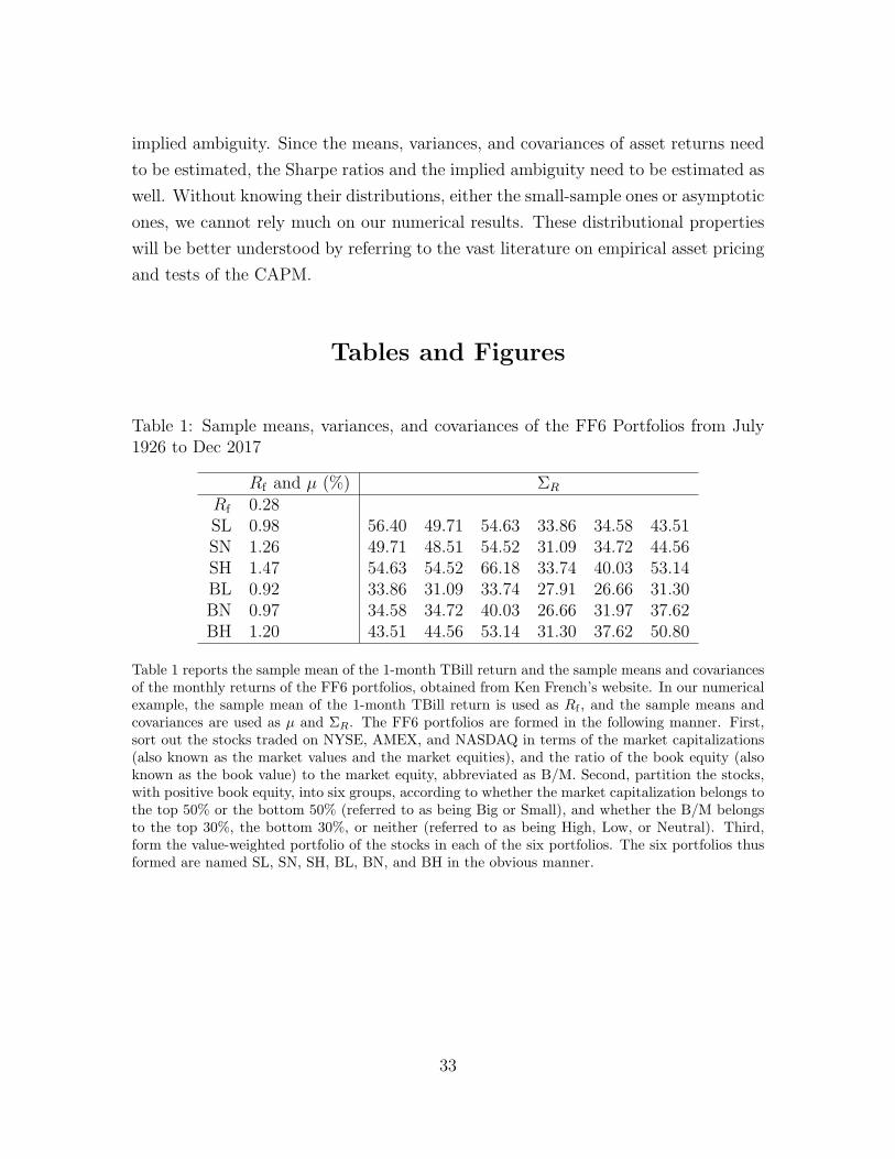
implied ambiguity. Since the means, variances, and covariances of asset returns need

to be estimated, the Sharpe ratios and the implied ambiguity need to be estimated as

well. Without knowing their distributions, either the small-sample ones or asymptotic

ones, we cannot rely much on our numerical results. These distributional properties

will be better understood by referring to the vast literature on empirical asset pricing

and tests of the CAPM.

Tables and Figures

Table 1: Sample means, variances, and covariances of the FF6 Portfolios from July1926 to Dec 2017

Rf and µ (%) ΣR

Rf 0.28SL 0.98 56.40 49.71 54.63 33.86 34.58 43.51SN 1.26 49.71 48.51 54.52 31.09 34.72 44.56SH 1.47 54.63 54.52 66.18 33.74 40.03 53.14BL 0.92 33.86 31.09 33.74 27.91 26.66 31.30BN 0.97 34.58 34.72 40.03 26.66 31.97 37.62BH 1.20 43.51 44.56 53.14 31.30 37.62 50.80

Table 1 reports the sample mean of the 1-month TBill return and the sample means and covariancesof the monthly returns of the FF6 portfolios, obtained from Ken French’s website. In our numericalexample, the sample mean of the 1-month TBill return is used as Rf , and the sample means andcovariances are used as µ and ΣR. The FF6 portfolios are formed in the following manner. First,sort out the stocks traded on NYSE, AMEX, and NASDAQ in terms of the market capitalizations(also known as the market values and the market equities), and the ratio of the book equity (alsoknown as the book value) to the market equity, abbreviated as B/M. Second, partition the stocks,with positive book equity, into six groups, according to whether the market capitalization belongs tothe top 50% or the bottom 50% (referred to as being Big or Small), and whether the B/M belongsto the top 30%, the bottom 30%, or neither (referred to as being High, Low, or Neutral). Third,form the value-weighted portfolio of the stocks in each of the six portfolios. The six portfolios thusformed are named SL, SN, SH, BL, BN, and BH in the obvious manner.

33

Table 2: CAPM alphas and betas of the FF6 portfolios and the weights in the tan-gency, value-weighted, equal-weighted, and GMV portfolios.

Tangency Value-weighted Equal-weighed GMV CAPM CAPM SharpePortfolio Portfolio Portfolio Portfolio alpha beta Ratio

SL -3.10 0.02 0.23 -0.56 -0.15 1.20 0.09SN 3.07 0.03 0.24 0.80 0.16 1.16 0.14SH 1.09 0.02 0.28 -0.34 0.27 1.30 0.15BL 1.96 0.51 0.11 0.87 -0.02 0.93 0.12BN -1.29 0.31 0.10 0.73 -0.02 0.99 0.12BH -0.73 0.11 0.04 -0.50 0.07 1.20 0.13ER 2.09 0.99 1.19 0.86SD 8.36 5.51 6.82 4.75SR 0.22 0.13 0.13 0.12

Table 2 reports the weights in each of the tangency, value-weighted, equal-weighed portfolio, andGMV (global minimum variance) portfolios. The weights in the tangency portfolio are computedfrom the sample means, variances, and covariances of the returns of the FF6 portfolios. The value-weighted portfolio is determined by the time-series averages of the weights of the market capitaliza-tions of the FF6 portfolios. The equal-weighed portfolio is determined by the time-series averages ofthe factions of numbers of the firms in each of the FF6 portfolio. The weights in the GMV portfolioare computed from the sample variances and covariances of the returns of the FF6 portfolios. Eachportfolio is normalized so that the coordinates add up to one. The expected returns (denoted asER), standard deviations (denoted as SD), and Sharpe ratios (denoted as SR) of the four portfoliosare also reported. Table 2 also reports the CAPM alpha, beta, and Sharpe ratio of the FF6 portfo-lios. The CAPM beta is computed using the value-weighted portfolio and the sample variances andcovariances. Then CAPM alpha is computed using the beta.

Table 3: The implied ambiguity, the Sharpe ratio, and the norm of pricing error

θ θ˚ ηθ˚ Sr pxq

Sr pxq

ˆ

αpxqJΣ´1R αpxq

αpxqJΣ´1R αpxq

˙12

Value-Weighted 0.0234 0.0130 8.2534 0.5934 0.8049Equal-Weighted 0.0196 0.0109 7.5018 0.6137 0.7895

GMV 0.0260 0.0143 9.3015 0.5680 0.8230

Table 3 reports the implied ambiguity and the corresponding coefficients of absolute risk aversionof the value-weighted, equal-weighed, and GMV portfolios in Table 2. The upper bound θ on thecoefficients of constant absolute risk aversion is defined in (15). The coefficients θ˚ of constant

absolute risk aversion and the implied ambiguity ηθ˚

are defined in Theorem 4. Sr pxqSr pxq

is the Sharpe ratio of each portfolio divided by the Shape ratio of the tangency portfolio x.`

αpxqJΣ´1R αpxqαpxqJΣ´1

R αpxq˘12

is the norm, defined in (28), of the vector of alphas if we useeach portfolio as the pricing factor, divided by the norm of the return of a portfolio x with a zeroexpected excess return.

34

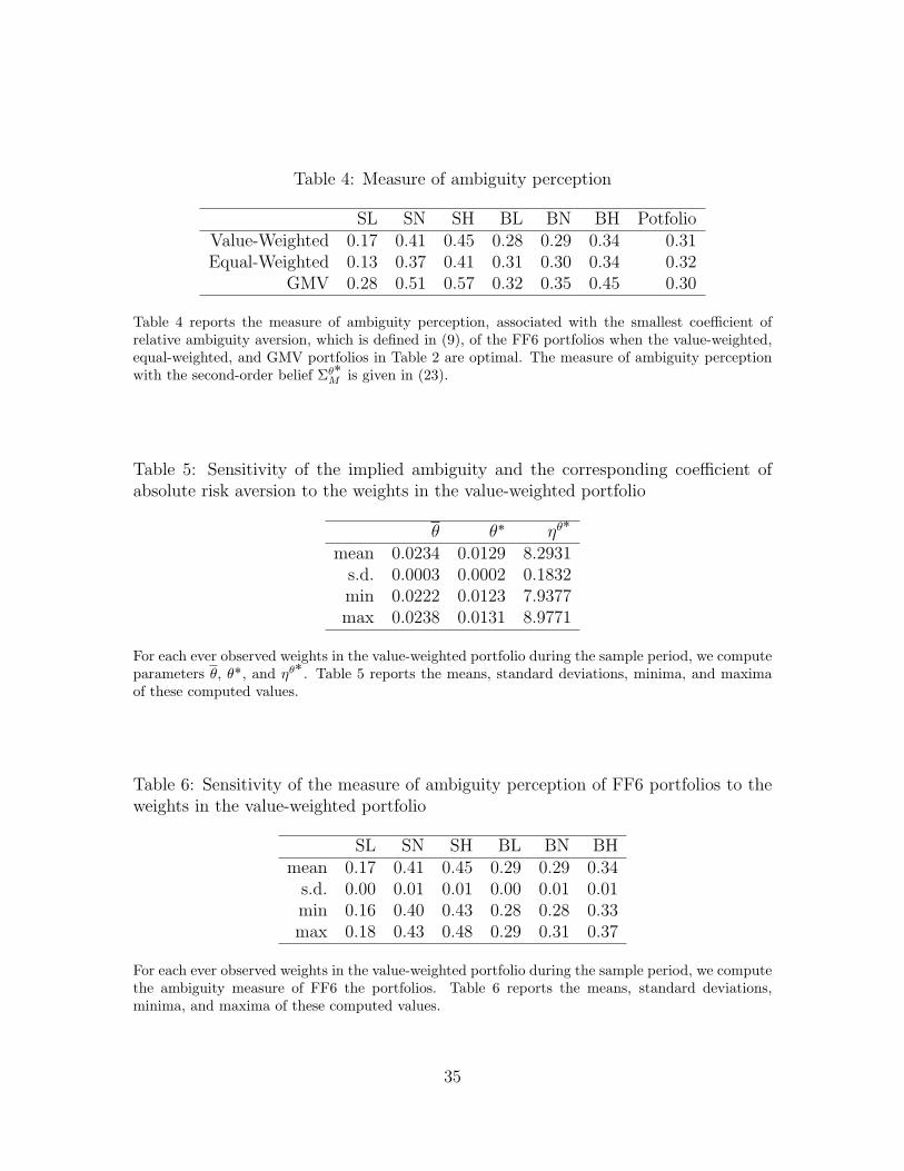
Table 4: Measure of ambiguity perception

SL SN SH BL BN BH PotfolioValue-Weighted 0.17 0.41 0.45 0.28 0.29 0.34 0.31Equal-Weighted 0.13 0.37 0.41 0.31 0.30 0.34 0.32

GMV 0.28 0.51 0.57 0.32 0.35 0.45 0.30

Table 4 reports the measure of ambiguity perception, associated with the smallest coefficient ofrelative ambiguity aversion, which is defined in (9), of the FF6 portfolios when the value-weighted,equal-weighted, and GMV portfolios in Table 2 are optimal. The measure of ambiguity perceptionwith the second-order belief Σθ˚

M is given in (23).

Table 5: Sensitivity of the implied ambiguity and the corresponding coefficient ofabsolute risk aversion to the weights in the value-weighted portfolio

θ θ˚ ηθ˚

mean 0.0234 0.0129 8.2931s.d. 0.0003 0.0002 0.1832min 0.0222 0.0123 7.9377max 0.0238 0.0131 8.9771

For each ever observed weights in the value-weighted portfolio during the sample period, we computeparameters θ, θ˚, and ηθ

˚. Table 5 reports the means, standard deviations, minima, and maxima

of these computed values.

Table 6: Sensitivity of the measure of ambiguity perception of FF6 portfolios to theweights in the value-weighted portfolio

SL SN SH BL BN BHmean 0.17 0.41 0.45 0.29 0.29 0.34s.d. 0.00 0.01 0.01 0.00 0.01 0.01min 0.16 0.40 0.43 0.28 0.28 0.33max 0.18 0.43 0.48 0.29 0.31 0.37

For each ever observed weights in the value-weighted portfolio during the sample period, we computethe ambiguity measure of FF6 the portfolios. Table 6 reports the means, standard deviations,minima, and maxima of these computed values.

35

Figure 1: Mean-variance efficiency frontier and the tangency portfolio

standard deviation

of the return

mean of the

return

tangency (TAN) portfolio

global minimum variance (GMV) portfolio riskless rate R

Obtained by a portfolio of stocks only

Figure 1 depicts the mean-variance efficiency frontier and the riskless return in the space of meansand standard deviations, and the highest Sharpe ratio, attained by the tangency portfolio.

Figure 2: Coefficients ηθ of relative ambiguity aversion as a function of the coefficientsθ of absolute risk aversion, and ambiguity measure of the FF6 and market portfolios

0.005 0.010 0.015 0.020

010

2030

4050

6070 eta_theta

0.005 0.010 0.015 0.020

0.0

0.1

0.2

0.3

0.4

0.5

0.6

0.005 0.010 0.015 0.020

0.0

0.1

0.2

0.3

0.4

0.5

0.6

0.005 0.010 0.015 0.020

0.0

0.1

0.2

0.3

0.4

0.5

0.6

0.005 0.010 0.015 0.020

0.0

0.1

0.2

0.3

0.4

0.5

0.6

0.005 0.010 0.015 0.020

0.0

0.1

0.2

0.3

0.4

0.5

0.6

0.005 0.010 0.015 0.020

0.0

0.1

0.2

0.3

0.4

0.5

0.6

0.005 0.010 0.015 0.020

0.0

0.1

0.2

0.3

0.4

0.5

0.6

SLSNSHBLBNBHVW

The left figure is the graph of the coefficients ηθ, which is defined in (19), of relative ambiguityaversion as a function of the coefficients θ of absolute risk aversion when the value-weighted portfolioin Table 2 is optimal. The right figure gathers the graphs of the ambiguity measures Amb p¨ |Σθ

M q

of the FF6 and market portfolios as functions of the coefficients of absolute risk aversion when thevalue-weighted portfolio in Table 2 is optimal. The ambiguity measure is given by equation (23).

36

A Lemmas and Proofs for Section 2

Proof of Lemma 1 By the properties of the moment generating function,

E“

uθ

`

xJR ` yRf

˘

|M‰

“ ´ expp´θyRfqE“

exp`

p´θxqJR˘

|M‰

“ ´ expp´θyRfq exp

ˆ

p´θxqJM `1

2pθxqJΣR|Mpθxq

˙

“ ´ exp

ˆ

´θ

ˆ

xJM ` Rfy ´θ

2xJΣR|Mx

˙˙

.

Then it follows from the definition of φγ,θ that

φγ,θ

`

E“

uθ

`

xJR ` yRf

˘

|M‰˘

“ ´ exp

ˆ

´γ

ˆ

xJM ` Rfy ´θ

2xJΣR|Mx

˙˙

.

Thus, again by the properties of the moment generating function,

Uγ,θpxJR ` yRfq “ Uγ,θpx

JR ` yRfqE

„

´ exp

ˆ

´γ

ˆ

xJM ` Rfy ´θ

2xJΣR|Mx

˙˙ȷ

“ ´ exp

ˆ

´γ

ˆ

Rfy ´θ

2xJΣR|Mx

˙˙

E“

exp`

p´γxqJM˘‰

“ ´ exp

ˆ

´γ

ˆ

Rfy ´θ

2xJΣR|Mx

˙˙

exp

ˆ

µJp´γxq `1

2p´γxqJΣMp´γxq

˙

“ uγ pVγ,θpx, yqq .

///

To prove Proposition 2, we need a lemma. To state it, let P P S N and consider

the problem of minimizing the quadratic form defined by P :

minwPRN zt0u

wJPw

w2. (30)

Denote a solution by w1. Next, let n ě 2 and w1, w2, . . . wn´1 belong to RN , and

consider the problem of minimizing the quadratic form subject to the constraint that

the solution must be orthogonal to w1, w2, . . . , wn´1:

minwPRN zt0u

wJPw

w2

s. t. wm ¨ w “ 0 for every m ď n ´ 1.

(31)

37

We say that a sequence pw1, w2, . . . , wNq of vectors in RN is a sequence of solutions

to (30) and (31) if w1, w2, . . . , wN are obtained iteratively by solving (30) and (31).

There is a sequence of solutions to the problems (31), because the objective functions

are continuous and the domains can be restricted to tw P RN | w “ 1u. Moreover,

for every sequence pw1, w2, . . . , wNq of solutions, pw1, w2, . . . , wNq is orthogonal and

wJ1 Pw1

w12

ďwJ

2 Pw2

w22

ď ¨ ¨ ¨ ďwJ

NPwN

wN2

for every n. Since the following lemma, which characterizes the eigenvectors and

eigenvalues of P , is well known,15 we omit the proof.

Lemma 3 1. For every sequence pw1, w2, . . . , wNq of solutions to the sequence of

problems (31) and for every n, wn is an eigenvector of P and its corresponding

eigenvalue is equal to wJnPwnwn2.

2. For every sequence pw1, w2, . . . , wNq of eigenvectors of P that is orthogonal and

of which the sequence of the corresponding eigenvalues is non-decreasing is a

sequence of solutions to the sequence of problems (31).

3. If w1, w2, . . . , wK are eigenvectors of P that correspond to distinct eigenvectors,

then pw1, w2, . . . , wKq is orthogonal.

Proposition 2 can be proved using this lemma as follows.

Proof of Proposition 2 Define P “ Σ´12ΞΣ´12. Since ΣM P S N , P P S N . More-

over, assume that w P RN , v P RN , λ P R and v “ Σ´12w. Then pvJΞvqpvJΣvq “

pwJPwqw2, and pΣ´1Ξqv “ λv if and only if Pw “ λw. Thus, parts 1 and 2 of this

proposition follow from parts 1 and 2 of Lemma 3. If, in addition, w1 P RN , v1 P RN ,

and v1 “ Σ´12w1, then vJΣv “ w ¨ w1. Thus, part 3 of this proposition follows from

part 3 of Lemma 3. It remains to prove part 4. Let λ be an eigenvalue of Q and v be

a corresponding eigenvector. Then ΣMv “ λΣRv. Thus vJΣMv “ λvJ

nΣRv, that is,

λ “vJΣMv

vJΣMv ` vJΣR|Mv.

15It is used, for example, in Campbell, Lo, and MacKinlay (1997, Section 6.4), in which theminimum is replaced by the maximum.

38

Since vJΣR|Mv ě 0, 0 ď λ ď 1. ///

B Proofs for Section 3

Proof of Theorem 1 Let Λ be the set of all eigenvalues of Q. It follows from

Proposition 2 that Λ Ă r0, 1s. For each λ P Λ, denote by Vλ the eigenspace that

correspond to λ. It also follows that Vλ is a linear subspace of RN , pVλqλPΛ is linearly

independent (that is, if vλ P Vλ for every λ P Λ andř

λPΛ vλ “ 0, then vλ “ 0 for

every λ P Λ), andř

λPΛ Vλ “ RN .

Then, for each λ P Λ, there is a vλ P Vλ such that ζp0q “ř

λPΛ vλ. Since ζp0q ‰ 0,

there is a λ P Λ such that vλ ‰ 0. Let tλ1, λ2, . . . , λKu be the set of all such λ’s. For

each k, write vk “ vλk, then ζp0q “

řKk“1 vk.

Since pI ` ηQqvk “ p1 ` ηλkqvk, pI ` ηQq´1vk “ p1 ` ηλkq´1vk. Thus,

ζpηq “ pI ` ηQq´1ζp0q “

Kÿ

k“1

pI ` ηQq´1vk “

Kÿ

k“1

1

1 ` λkηvk.

///

Proof of Proposition 1 We first prove the following fact: letK be a positive integer

and suppose that there are K distinct nonnegative numbers λ1, λ2, . . . , λK such that

rank pλkΣR ´ ΣMq ă N for every k andřK

k“1 rank pλkΣR ´ ΣMq “ pK ´ 1qN . Then,

for every k, there exists a vk P Ker pλkΣR ´ ΣMq such that, for every η ą ´1, ζpηq “řK

k“1p1`λkηq´1vk. Indeed, by the definition of Q, Ker pλkΣR´ΣMq “ Ker pλkIN ´Qq

and dimKer pλkIN ´Qq “ N ´ rank pλkΣR ´ΣMq ą 0. Thus Ker pλkΣR ´ΣMq is the

eigenspace of Q that corresponds to eigenvalue λk. Moreover,

Kÿ

k“1

dimKer pλkΣR ´ ΣMq “

Kÿ

k“1

pN ´ rank pλkΣR ´ ΣMqq “ KN ´ pK ´ 1qN “ N.

Thus RN coincides with the direct sum of the K eigenspaces Ker pλkΣR ´ΣMq. Thus

λ1, λ2, . . . , λK are the eigenvalues of Q. Part 1 therefore follows from Theorem 1.

1. This is a special case of the above fact with K “ 1.

2. Since rankΣM ă N and rank pΣR ´ ΣMq ă N , this is a special case of the

above fact with K “ 2 and tλ1, λ2u “ t0, λu.

39

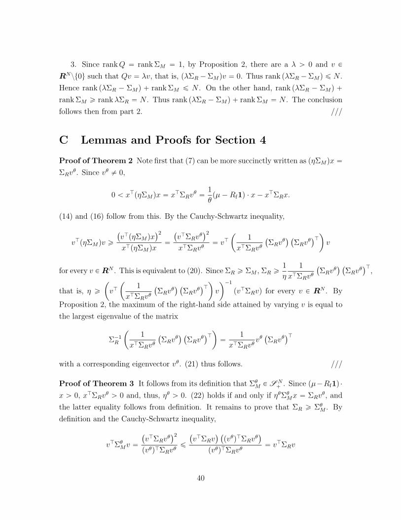
3. Since rankQ “ rankΣM “ 1, by Proposition 2, there are a λ ą 0 and v P

RNzt0u such that Qv “ λv, that is, pλΣR ´ ΣMqv “ 0. Thus rank pλΣR ´ ΣMq ď N .

Hence rank pλΣR ´ ΣMq ` rankΣM ď N . On the other hand, rank pλΣR ´ ΣMq `

rankΣM ě rankλΣR “ N . Thus rank pλΣR ´ ΣMq ` rankΣM “ N . The conclusion

follows then from part 2. ///

C Lemmas and Proofs for Section 4

Proof of Theorem 2 Note first that (7) can be more succinctly written as pηΣMqx “

ΣRvθ. Since vθ ‰ 0,

0 ă xJpηΣMqx “ xJΣRvθ “

1

θpµ ´ Rf1q ¨ x ´ xJΣRx.

(14) and (16) follow from this. By the Cauchy-Schwartz inequality,

vJpηΣMqv ě

`

vJpηΣMqx˘2

xJpηΣMqx“

`

vJΣRvθ˘2

xJΣRvθ“ vJ

ˆ

1

xJΣRvθ`

ΣRvθ˘ `

ΣRvθ˘J

˙

v

for every v P RN . This is equivalent to (20). Since ΣR ě ΣM , ΣR ě1

η

1

xJΣRvθ`

ΣRvθ˘ `

ΣRvθ˘J

,

that is, η ě

ˆ

vJ

ˆ

1

xJΣRvθ`

ΣRvθ˘ `

ΣRvθ˘J

˙

v

˙´1

pvJΣRvq for every v P RN . By

Proposition 2, the maximum of the right-hand side attained by varying v is equal to

the largest eigenvalue of the matrix

Σ´1R

ˆ

1

xJΣRvθ`

ΣRvθ˘ `

ΣRvθ˘J

˙

“1

xJΣRvθvθ

`

ΣRvθ˘J

with a corresponding eigenvector vθ. (21) thus follows. ///

Proof of Theorem 3 It follows from its definition that ΣθM P S N

` . Since pµ´Rf1q ¨

x ą 0, xJΣRvθ ą 0 and, thus, ηθ ą 0. (22) holds if and only if ηθΣθ

Mx “ ΣRvθ, and

the latter equality follows from definition. It remains to prove that ΣR ě ΣθM . By

definition and the Cauchy-Schwartz inequality,

vJΣθMv “

`

vJΣRvθ˘2

pvθqJΣRvθď

`

vJΣRv˘ `

pvθqJΣRvθ˘

pvθqJΣRvθ“ vJΣRv

40

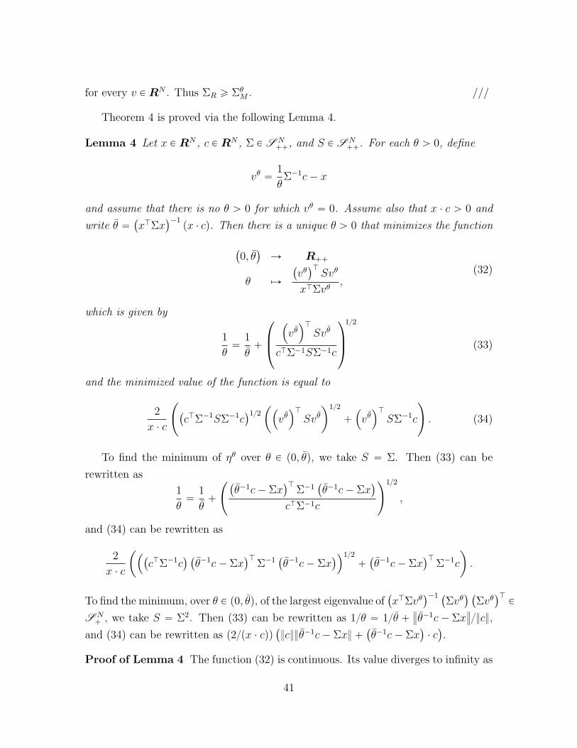
for every v P RN . Thus ΣR ě ΣθM . ///

Theorem 4 is proved via the following Lemma 4.

Lemma 4 Let x P RN , c P RN , Σ P S N``, and S P S N

``. For each θ ą 0, define

vθ “1

θΣ´1c ´ x

and assume that there is no θ ą 0 for which vθ “ 0. Assume also that x ¨ c ą 0 and

write θ “`

xJΣx˘´1

px ¨ cq. Then there is a unique θ ą 0 that minimizes the function

`

0, θ˘

Ñ R``

θ ÞÑ

`

vθ˘J

Svθ

xJΣvθ,

(32)

which is given by

1

θ“

1

θ`

¨

˚

˝

´

vθ¯J

Svθ

cJΣ´1SΣ´1c

˛

‹

‚

12

(33)

and the minimized value of the function is equal to

2

x ¨ c

˜

`

cJΣ´1SΣ´1c˘12

ˆ

´

vθ¯J

Svθ˙12

`

´

vθ¯J

SΣ´1c

¸

. (34)

To find the minimum of ηθ over θ P p0, θq, we take S “ Σ. Then (33) can be

rewritten as

1

θ“

1

θ`

˜

`

θ´1c ´ Σx˘J

Σ´1`

θ´1c ´ Σx˘

cJΣ´1c

¸12

,

and (34) can be rewritten as

2

x ¨ c

ˆ

´

`

cJΣ´1c˘ `

θ´1c ´ Σx˘J

Σ´1`

θ´1c ´ Σx˘

¯12

``

θ´1c ´ Σx˘J

Σ´1c

˙

.

To find the minimum, over θ P p0, θq, of the largest eigenvalue of`

xJΣvθ˘´1 `

Σvθ˘ `

Σvθ˘J

P

S N` , we take S “ Σ2. Then (33) can be rewritten as 1θ “ 1θ `

›

›θ´1c ´ Σx›

›c,

and (34) can be rewritten as p2px ¨ cqq`

cθ´1c ´ Σx ``

θ´1c ´ Σx˘

¨ c˘

.

Proof of Lemma 4 The function (32) is continuous. Its value diverges to infinity as

41

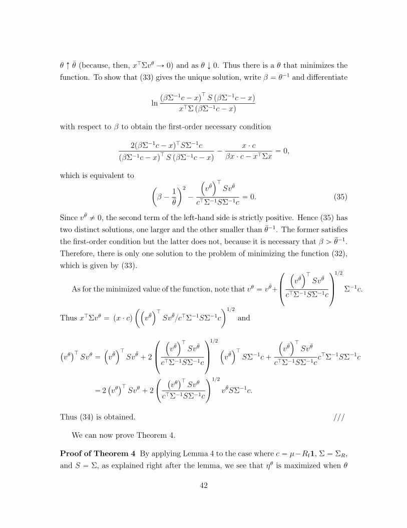
θ Ò θ (because, then, xJΣvθ Ñ 0) and as θ Ó 0. Thus there is a θ that minimizes the

function. To show that (33) gives the unique solution, write β “ θ´1 and differentiate

lnpβΣ´1c ´ xq

JS pβΣ´1c ´ xq

xJΣ pβΣ´1c ´ xq

with respect to β to obtain the first-order necessary condition

2pβΣ´1c ´ xqJSΣ´1c

pβΣ´1c ´ xqJ S pβΣ´1c ´ xq

´x ¨ c

βx ¨ c ´ xJΣx“ 0,

which is equivalent toˆ

β ´1

θ

˙2

´

´

vθ¯J

Svθ

cJΣ´1SΣ´1c“ 0. (35)

Since vθ ‰ 0, the second term of the left-hand side is strictly positive. Hence (35) has

two distinct solutions, one larger and the other smaller than θ´1. The former satisfies

the first-order condition but the latter does not, because it is necessary that β ą θ´1.

Therefore, there is only one solution to the problem of minimizing the function (32),

which is given by (33).

As for the minimized value of the function, note that vθ “ vθ`

¨

˚

˝

´

vθ¯J

Svθ

cJΣ´1SΣ´1c

˛

‹

‚

12

Σ´1c.

Thus xJΣvθ “ px ¨ cq

ˆ

´

vθ¯J

SvθcJΣ´1SΣ´1c

˙12

and

`

vθ˘J

Svθ “

´

vθ¯J

Svθ ` 2

¨

˚

˝

´

vθ¯J

Svθ

cJΣ´1SΣ´1c

˛

‹

‚

12

´

vθ¯J

SΣ´1c `

´

vθ¯J

Svθ

cJΣ´1SΣ´1ccJΣ´1SΣ´1c

“ 2`

vθ˘J

Svθ ` 2

˜

`

vθ˘J

Svθ

cJΣ´1SΣ´1c

¸12

vθSΣ´1c.

Thus (34) is obtained. ///

We can now prove Theorem 4.

Proof of Theorem 4 By applying Lemma 4 to the case where c “ µ´Rf1, Σ “ ΣR,

and S “ Σ, as explained right after the lemma, we see that ηθ is maximized when θ

42

is equal to

¨

˝

1

θ`

˜

`

θ´1pµ ´ Rf1q ´ ΣRx˘J

Σ´1R

`

θ´1pµ ´ Rf1q ´ ΣRx˘

pµ ´ Rf1qJΣ´1R pµ ´ Rf1q

¸12˛

‚

´1

(36)

and, then, ηθ is equal to

2

x ¨ pµ ´ Rf1qˆ

„

´

`

θ´1pµ ´ Rf1q ´ ΣRx˘J

Σ´1R

`

θ´1pµ ´ Rf1q ´ ΣRx˘

¯12

`

pµ ´ Rf1qJΣ´1R pµ ´ Rf1q

˘12`

`

θ´1pµ ´ Rf1q ´ ΣRx˘J

Σ´1R pµ ´ Rf1q

ȷ

. (37)

Note here that`

θ´1pµ ´ Rf1q ´ ΣRx˘J

Σ´1R

`

θ´1pµ ´ Rf1q ´ ΣRx˘

is equal to

θ´2 pSr pxqq2

´ 2θ´1x ¨ pµ ´ Rf1q ` xJΣRx

“ θ´2 pSr pxqq2

´ xJΣRx “ θ´2`

pSr pxqq2

´ pSr pxqq2˘

.

Thus,

`

θ´1pµ ´ Rf1q ´ ΣRx˘J

Σ´1R

`

θ´1pµ ´ Rf1q ´ ΣRx˘

pµ ´ Rf1qJ Σ´1

R pµ ´ Rf1q“

1

θ2

˜

1 ´

ˆ

Sr pxq

Sr pxq

˙2¸

.

Thus, (36) is equal to

¨

˝

1

θ`

1

θ

˜

1 ´

ˆ

Sr pxq

Sr pxq

˙2¸12

˛

‚

´1

“θ

1 `

˜

1 ´

ˆ

Sr pxq

Sr pxq

˙2¸12

,

and (37) is equal to

2

x ¨ pµ ´ Rf1q

´

θ´1`

pSr pxqq2

´ pSr pxqq2˘12

Sr pxq ` θ´1 pSr pxqq2

´ x ¨ pµ ´ Rf1q

¯

“2

ˆ

1

pSr pxqq2

`

pSr pxqq2

´ pSr pxqq2˘12

Sr pxq `1

pSr pxqq2pSr pxqq

2´ 1

˙

“2

ˆ

Sr pxq

Sr pxq

˙2˜

1 ´

ˆ

Sr pxq

Sr pxq

˙2¸12

¨

˝1 `

˜

1 ´

ˆ

Sr pxq

Sr pxq

˙2¸12

˛

‚.

43

Since

¨

˝1 `

˜

1 ´

ˆ

Sr pxq

Sr pxq

˙2¸12

˛

‚

¨

˝1 ´

˜

1 ´

ˆ

Sr pxq

Sr pxq

˙2¸12

˛

‚“

ˆ

Sr pxq

Sr pxq

˙2

,

this is equal to the right hand side of (25). ///

References

[1] Ahn, D., Choi, S., Gale, D. and Kariv, S. 2014, Estimating ambiguity aver-

sion in a portfolio choice experiment. Quantitative Economics 5:195-223. doi:

10.3982/QE243

[2] Ang, A., 2014, Portfolio Management: A Systematic Approach to Factor Invest-

ing, Oxford University Press.

[3] Attanasi, G., Gollier, C., Montesano, A., and Pace, N. 2014. Eliciting ambiguity

aversion in unknown and in compound lotteries: A smooth ambiguity model

experimental study. Theory and decision 77(4): 485-530.

[4] Bossaerts, P., P. Ghirardato, S. Guarnaschelli, and W.R. Zame, 2010, Ambiguity

in asset markets: Theory and experiment, Review of Financial Studies 23: 1325–

1359.

[5] Canner, N., N. G. Mankiw, and D. N. Weil, 1997, An asset allocation puzzle,

American Economic Review 87: 181–191.

[6] Campbell, J. Y., A. Lo, and C. MacKinlay. 1997, The Econometrics of Financial

Markets. Princeton University Press.

[7] Collard, F., S. Mukerji, K. Sheppard, and J. Tallon, 2018, Ambiguity and the

historical equity premium, Quantitative Economics 945–993.

[8] Duffie, D., 2001, Dynamic Asset Pricing Theory, third edition, Princeton Uni-

versity Press.

[9] Ellsberg, D., 1961, Risk, ambiguity, and the Savage axiom, Quarterly Journal of

Economics 75, 643–669.

44

[10] Epstein, L. G. 2010, A paradox for the “smooth ambiguity” model of preference,

Econometrica 78: 2085–2099.

[11] Fama, E. F., 1996, Multifactor portfolio efficiency and multifactor asset pricing,

Journal of Financial and Quantitative Analysis 31, 441–465.

[12] Fama, Eugene F., and Kenneth R. French. 1992. The cross-section of expected

stock returns. it Journal of finance 47(2):427-465.

[13] Ghirardato, P., F. Maccheroni, and M. Marinacci, 2004, Differentiating ambigu-

ity and ambiguity aversion, Journal of Economic Theory 118, 133–173.

[14] Gibbons, M. R., S. A. Ross, and J. Shanken, 1989, A test of the efficiency of a

given portfolio, Econometrica 57, 1121–1152.

[15] Gilboa, I., and D. Schmeidler. 1989. Maxmin Expected Utility with Non-Unique

Prior, Journal of Mathematical Economics 18:141–153.

[16] Hansen, L. P., and R. Jagannathan, 1997, Assessing specification errors in

stochastic discount factor models, Journal of Finance 52, 557–590.

[17] Klibanoff, P., M. Marinacci, and S. Mukerji. 2005. A smooth model of decision

making under ambiguity. Econometrica 73:1849–1892.

[18] Maccheroni, F., M. Marinacci, and D. Ruffino. 2013. Alpha as Ambiguity: Ro-

bust Mean-Variance Portfolio Analysis. Econometrica 81:1075–1113.

[19] Harry Markowitz, 1952, Portfolio selection, Journal of Finance 7, 77–91.

[20] Rajnish Mehra and Edward C. Prescott, 1985, The equity premium: A puzzle,

Journal of Monetary Economics 15, 145–161.

[21] Shanken, J., 1987, Multivariate proxies and asset pricing relations: Living with

the Roll critique, Journal of Financial Economics 18, 91–110.

[22] Thimme, J., and C. Volkert, 2015, Ambiguity in the cross-section of expected

returns: An empirical assessment, Journal of Business and Economic Statistics

33, 418–429.

[23] Tobin, J., 1958, Liquidity preference as behavior towards risk, Review of Eco-

nomic Studies 25, 65–86.

45