kier discussion paper series · matsushima, takako fujiwara-greve, satoru takahashi, masatoshi...
TRANSCRIPT
KIER DISCUSSION PAPER SERIES
KYOTO INSTITUTE OF
ECONOMIC RESEARCH
KYOTO UNIVERSITY
KYOTO, JAPAN
Discussion Paper No.924
“A Dynamic Mechanism Design for Scheduling with Different Use Lengths”
Ryuji Sano
June 2015

A Dynamic Mechanism Design for Scheduling with
Different Use Lengths∗
Ryuji Sano†
Institute of Economic Research, Kyoto University
June 12, 2015
Abstract
This paper considers a dynamic allocation problem in which many perishable
goods are allocated at each period. Agents want to keep winning goods for more
than one period to make profits. We consider efficient and optimal mechanisms
when the seller offers simple long-term contracts. The dynamic VCG mechanism
achieves efficient allocations. The expected revenue is maximized by the virtual
welfare maximization. In the single unit case, price discounts for long-stay
agents can be optimal under certain distributions. Both the efficient and optimal
mechanisms are implemented by a simple “handicap auction” in the binary
length case.
Keywords: dynamic mechanism design, online mechanism, optimal auction
JEL classification: C73, D44, D82
∗First draft: November 2012. I thank Michihiro Kandori, Fuhito Kojima, Makoto Yokoo, Hitoshi
Matsushima, Takako Fujiwara-Greve, Satoru Takahashi, Masatoshi Tsumagari, Yosuke Yasuda,
Daisuke Oyama, Takashi Kunimoto, and the seminar and conference participants at Keio University,
National University of Singapore, Okayama University, the JEA Spring Meeting, Meeting of Society
for Social Choice and Welfare, and INFORMS annual meeting 2014 for their helpful comments
and suggestions. This research was supported by a Grant-in-Aid for Young Scientists (KAKENHI
25780132) from Japan Society for the Promotion of Sciences (JSPS).†Institute of Economic Research, Kyoto University, Yoshida-Honmachi, Sakyo-ku, Kyoto 606-
8501, Japan. Telephone: +81-75-7537122. E-mail: [email protected]
1

1 Introduction
This paper considers a dynamic allocation problem where a seller allocates many
perishable objects at each period. A motivating example is an on-line scheduling
problem. Suppose that there are a number of facilities such as city halls, hotel
rooms, or shared computer servers, and time slots to use such facilities are allocated
at each time. Potential users randomly arrive over time and often want to use the
facilities for a long time. For example, a conference or an exhibition would be held
at a hotel or a convention center for several days or a week. People would like to stay
at a hotel for several nights, or a computer job would need a long processing time to
complete on a server. A similar environment would also be considered in electricity
markets, in which an electricity supplier or a power plant signs a big contract with
firms, factories, and retailers over time. People need the object for different periods
to be satisfied, and the necessary duration is in general private information of each
person along with the valuation.
The seller faces tradeoff between revenue from current long-stay buyers and that
from potential future buyers. The seller often needs to sign long-term contracts for
buyers and reserve future slots for them in advance. Although a long-term contract
might be contingent on future events, such a complex contract is often difficult in
practical situations. Only simple incomplete contracts that are not contingent on
future events are available in many real situations. In such a case, how can the seller
achieve the efficient outcome? And, how can she maximize her expected revenue?
This paper applies a standard mechanism design to this problem. We charac-
terize incentive compatible mechanisms, and provide an efficient mechanism and a
revenue-maximizing mechanism in our domain of mechanisms. Given a period length,
incentive compatibility requires that the allocation policy for an agent is increasing
in his valuation, and that the payment is determined by the envelope theorem. In
addition, to ensure reporting true lengths, the allocation policy needs to satisfy a
weak notion of monotonicity on lengths. We show that these conditions are also
sufficient for incentive compatibility.
2
Standard techniques provide the efficient mechanism and the revenue-maximizing
mechanism. The efficient mechanism is provided as a straightforward extension of
the Vickrey-Clarke-Groves (VCG) mechanism. Each agent pays the expected exter-
nality to the other current and future agents. The revenue-maximizing (optimal)
mechanism is provided as in Myerson (1981) and Riley and Samuelson (1981). The
optimal allocation policy maximizes the discounted virtual valuations under a mono-
tone hazard rate condition.
We then consider two specific cases. First, we consider a single unit case. With
certain distribution conditions, the optimal allocation policy is distorted in such a
way that long-stay agents are more favored than in the efficient allocation policy.
In addition, the optimal posted prices exhibit volume discounts for long-stay agents,
as is sometimes observed in the real world. However, such long-stay discounts are
not robust. The existence of long-stay discounts or premium depends on the type
distribution and population dynamics.
Second, we consider the case where agents stay at most for two periods. We show
that the concavity of the maximum social welfare function in terms of current supply
units. As a result, the efficient allocation policy is implemented by simple multi-
unit uniform price auctions with proper handicaps to long-stay agents. Analogously,
revenue maximization is done by multi-unit uniform price auctions with reserve prices
and handicaps.
1.1 Related Literature
In recent years, a number of studies consider dynamic auction design.1 Dynamic
auction design in an environment where agents strategically arrive and depart is
often called online mechanism design, and has been investigated in the fields of
computer science and operations research (Lavi and Nisan, 2000).
Parkes and Singh (2003), Mierendorff (2009), and Pai and Vohra (2013) consider
an allocation problem of durable goods, such as air ticket sales and hotel reservations.
1See Bergemann and Said (2011) and Parkes (2007) for a review.
3

Buyers arrive over time, stay for several periods, and participate in auctions during
their stay. They buy a good at most once in their stay. Parkes and Singh (2003)
extend the VCG mechanism to the case where buyers strategically choose their arrival
and departure times. Mierendorff (2009) and Pai and Vohra (2013) investigate the
optimal mechanism.
Hajiaghayi et al. (2005) and Parkes (2007) consider a perishable goods case such
as scheduling of facilities in the presence of strategic arrivals and departures. They
consider incentive compatible mechanisms and investigate the efficiency of an allo-
cation policy. In the literature of machine job scheduling, Porter (2004) considers
a dynamic mechanism with heterogeneous job lengths. Kittsteiner and Moldovanu
(2005) study queueing mechanism using auctions under stochastic arrivals of jobs
with heterogeneous waiting cost and processing time.
Dizdar et al. (2011) consider a problem closely related to ours. They consider
a durable goods sale (knapsack problem) to a sequence of short-lived buyers who
have multiple-unit demands. They characterize the implementability of determinis-
tic allocation rule with two-dimensional type of value and demand volume. Then,
they examine revenue maximization and sufficient conditions for the regularity of
the problem. For a difference from their characterization result, we allow random
allocation rule to some extent whereas they limit attention on deterministic rules
and strategy-proofness.
For other models with random arrivals of agents, Vulcano et al. (2002) and Ger-
shkov and Moldovanu (2009, 2010) consider the efficient or optimal durable goods
sales in which agents are impatient and short-lived. Board and Skrzypacz (2010) also
consider durable goods sales in which agents are patient and stay until the deadline
of the sale. Said (2012) considers a perishable goods case. Buyers arrive at random
and stay through the next period with a positive probability common among buy-
ers. Said shows that the outcomes in the efficient and optimal mechanisms can be
achieved by repeated ascending auctions in a perfect Bayesian equilibrium.
Some studies examine a similar dynamic allocation problem with dynamic in-
4

formation. Bergemann and Valimaki (2010) consider a dynamic allocation problem
with fixed agents whose types fluctuate over time. They formulate an efficient mech-
anism by extending the VCG mechanism. Athey and Segal (2013) consider a similar
situation and provide an efficient budget-balancing mechanism. Pavan et al. (2014)
characterize incentive compatibility and provide revenue equivalence in a dynamic
information model.
The remainder of the paper is organized as follows. In section 2, we provide a
model of the time-slot scheduling problem. We characterize incentive compatibility
and show a revenue equivalence. In section 3, we consider the efficient mechanism
design. We show that truthful reporting is a dominant strategy in the dynamic
VCG mechanism. In section 4, we consider the revenue maximization for the seller.
We show that the optimal allocation policy maximizes virtual welfare under the
monotone hazard rate condition. In section 5, we focus on a single unit case. We
show that with a certain condition, the optimal allocation is distorted in such a way
that long-stay agents are more favored. In addition, the optimal posted prices exhibit
volume discounts for long-stay agents. In section 6, we examine the allocation policy
in the case where agents stay at most for two periods. The efficient and optimal
outcomes are implemented by a simple handicap auction. Section 7 concludes the
paper.
2 Model
We consider an environment with independent and private values in a discrete-time
model. K identical objects, for example, time slots of a city hall or facilities, are
supplied at each period t = 1, . . . , T . For simplicity, we consider infinite horizon:
T = ∞. Objects are non-storable and perish at the end of each period. At each
period, a finite number of agents enter the mechanism. The set of entrants at t is
denoted by N t, and the number of entrants |N t| is an i.i.d. random variable at each
period. Each agent at each period is ex ante homogeneous and wants to own at most
one unit of the object at a period. The set of agents having entered by t is denoted
5
by N t ≡∪
s≤t N s. An allocation at t is denoted by at = (ati)i∈N t . An allocation
ati ∈ [0, 1] for i denotes the probability of obtaining the object at t. An allocation
at is said to be feasible at t if∑
i ati ≤ K and at
i = 0 for any i who is not in the
mechanism at t. Let ati ∈ {0, 1} be the realized allocation for i at t.
Agents and the seller discount future payoffs by a common factor δ ∈ (0, 1). Each
agent i has his private information θi ≡ (Vi, li) ∈ [0, V ]×{1, . . . , L} ≡ Θi. Agent i of
type θi = (Vi, li) stays in a mechanism for at least li periods. Given a deterministic
sequence of allocations and payments, the utility of i ∈ N t evaluated at t is given by
ui =
Vi −
∑∞s=t δs−tps
i if asi = 1 for ∀s ∈ {t, . . . , t + li − 1},
−∑∞
s=t δs−tpsi otherwise,
(1)
where psi denotes i’s payment at s. Agent i earns a total profit Vi only if he owns the
object for li periods of time.2 Otherwise, agent i earns zero. We call Vi, valuation
type and li, length type. Each agent’s type θi is independently drawn from an identical
distribution F on Θi. Let F (·|li) be the cumulative distribution function conditional
on li. Given any li, F (·|li) has a density function f(·|li) > 0 for all Vi.3
The seller offers a long-term contract to each agent. Each agent signs only one
contract when he enters a mechanism.4 There is no renegotiation and a contract is
never revised or interrupted before its expiration. A contract for i at t, zti , specifies
a sequence of allocations and payments.
We restrict the domain of contracts to simple contracts that depend only on the
current history. We assume that a contract is defined as zti ≡ (ai,mi, Pi), where
ai ∈ [0, 1] specifies a (random) goods allocation, mi denotes a contract term, and
Pi =∑
s≥t δs−tpsi is total payment. Contract term mi is assumed to be determinis-
2Note that total profit Vi is evaluated at t. An alternative definition of the (expected) utility is
ui = ati · at+1
i · · · · · at+li−1i Vi −
X
s≥t
δs−tpsi .
3We may allow upper bound of valuations to depend on length types. Then, the conditional
density f(·|li) > 0 is assumed in the domain of values for each li.4If an agent rejects a contract, then he leaves the mechanism and gets payoff 0.
6

tic. Moreover, the admissible sequences of realized allocations (ati, . . . , a
t+mi−1i ) are
limited to (1, . . . , 1) and (0, . . . , 0). An allocation ai is the probability assigned to
the sequence (1, . . . , 1). In other words, agent i obtains the goods with a probability
of ai at his entry period t, and the realized allocation ati at t is allocated with prob-
ability 1 in the later periods. We take care of the total payment Pi instead of the
sequence of payments because there is a degree of freedom. The set of admissible
contracts for i is denoted by Zi ≡ [0, 1] × {1, . . . , L} × R. The set of bundles of
contracts at t is denoted by Zt ≡ ×i∈N tZi. For contract zti = (ai, mi, Pi), we use
the following notations for the corresponding components: ai(zti) = ai, mi(zt
i) = mi,
and Pi(zti) = Pi. The realized allocation from zt
i is denoted by ai(zti).
2.1 Dynamic Direct Mechanisms
We assume that each agent does not manipulate the arrival time. However, they
may manipulate their period lengths. We also assume that each agent does not ob-
serve past history or the number of current agents N t when making a report. This
assumption would be natural in many practical situations such as facility scheduling
and hotel room assignments. The assumption can also be interpreted as the case
where the seller hides past events so that agents’ incentive constraints are the weak-
est. One might consider the case in which agents observe some information about
past events. In such a case, an incentive constraint is necessary for every history.
We will see that the results of the paper hold even in such cases.
We apply the revelation principle and limit our attention to direct mechanisms.
Each agent reports the type to the seller at his entry. Then, the seller offers a
contract to each current entrant just once.
At each t, each entrant i ∈ N t makes a report γti = (Vi, li) ∈ Θi. The profile of
types at t is denoted by θt ≡ (θi)i∈Nt . The seller makes a contract for each i ∈ N t
based on the vector of reports γt ∈ Θt ≡∏
i∈Nt Θi and history up to t,
ht = (N1; γ1, z1, N2; . . . ; γt−1, zt−1, N t).
7
Let Ht be the set of possible history at t. A mechanism is denoted by {zt}∞t=1, where
zt : Θt × Ht → Zt.
A mechanism is feasible if zti = ∅ for all i 6∈ N t and if
∑i∈Nt ai(zt
i) ≤ Kt, where Kt
denotes the number of units available for the current entrants.5
For a profile of reports γt = (γtj)j∈Nt at t, an entrant i at t earns payoff
ui(γt, θi, ht) = ai(zti(γ
t, ht))I{mi(zti )≥li}Vi − Pi(zt
i(γt, ht)), (2)
where I denotes the indicator function. For the verifiability of contracts, we as-
sume that agents observe the history after the enforcement of their contracts. Let
Ui(θt, ht) ≡ ui((θi, θt−i), θi, ht), which indicates i’s payoff when every entrant at t
reports true information.
A bidder’s strategy is a mapping γi : Θi → Θi. Given that the others report
their true types, agent i ’s interim expected payoff is
πi(γti , θi) = E[ui(γt
i , θt−i, θi, ht)]
= αi(γti , li)Vi − qi(γt
i ),(3)
where
αi(γti , li) = E
[ai(zt
i(γti , θ
t−i, ht))I{mi(zt
i )≥li}]
(4)
and
qi(γti ) = E
[Pi(zt
i(γti , θ
t−i, ht))
]. (5)
Let Πi(θi) ≡ πi(θi, θi), which denotes the expected payoff when i reports his true in-
formation. Note that agent i’s winning probability αi depends on i’s true length type
li through the indicator function. Abusing notations, let αi(Vi, li) ≡ αi((Vi, li), li),
which indicates the winning probability when reporting the true length type.
Incentive compatibility and individual rationality are defined in a standard man-
ner.
5See section 3 for a formal definition of Kt.
8

Definition 1 A dynamic direct mechanism is (Bayesian) incentive compatible if for
all i, all t, all θi, and all γti ,
Πi(θi) ≥ πi(γti , θi).
A mechanism is individually rational if for all i, all t, and all θi, Πi(θi) ≥ 0.
Definition 2 A dynamic direct mechanism is dominant strategy incentive compatible
if for all i, all t, all ht, all θ, and all γti ,
Ui(θt, ht) ≥ ui((γti , θ
t−i), θi, ht).
Note that by the ex post availability of history, dominant strategy incentive com-
patibility is a little stronger than the standard definition in the sense that incentive
compatibility is imposed for every history.
2.2 Characterization of Incentive Compatibility
We characterize incentive compatibility and show the revenue equivalence. We limit
our attention to mechanisms such that contract terms are equal to the agents’ re-
ported lengths.
Definition 3 A dynamic direct mechanism is exact if it satisfies mi(zi(θt, ht)) = li
for all t, all ht, all i ∈ N t, and all θt.6
In an exact mechanism, every contract term is determined by the reported length.
This restriction would be natural and does not lose generality. It is easy to verify
that for any mechanism, there exists an equivalent exact mechanism that gives the
same payoffs and revenue.
Lemma 1 For any mechanism {zt}, there exists an equivalent exact mechanism that
gives the same payoffs for agents and revenue for the seller.
Proof. All proofs are in Appendix.
6The term “exactness” follows Lehmann et al. (2002) in the literature of multi-object auctions.
9

Hereafter, we focus on exact mechanisms. Incentive compatibility is characterized
by two separated monotonicity constraints. Similar results are found in Dizdar et
al. (2011), Pai and Vohra (2013) and Mierendorff (2009) in different settings.
Proposition 1 An exact dynamic direct mechanism is incentive compatible if and
only if for all i,
1. αi(Vi, li) is weakly increasing in Vi for every li,
2.∫ Vi
0 αi(ν, li)dν is weakly decreasing in li for every Vi, and
3. there exists a constant Πi, and
Πi(θi) = Πi +∫ Vi
0αi(ν, li)dν (6)
for all Vi and all li.
Preceding studies introduce a stronger notion of monotonicity of allocation policy,
which requires that allocation for an agent is monotone in both valuation and length.
We introduce a similar concept in our model. Given a mechanism {zt}, the allocation
policy is denoted by at : Θt × Ht → [0, 1]Nt
and
ati(θ
t, ht) ≡ ai(zti(θ
t, ht)).
Definition 4 An allocation policy is said to be monotone if for all i, ati(θ
t, ht) is
weakly increasing in Vi and weakly decreasing in li.
Note that incentive compatibility does not require the allocation policy to be
monotone in length. Proposition 1 implies that any monotone allocation policy is
implementable.7
Corollary 1 If an allocation policy is monotone, then there exists a payment scheme
that induces incentive compatibility.7Bikhchandani et al. (2006) show that in a multi-dimensional model, a deterministic allocation
rule is implemented in dominant strategy if and only if it is weakly monotone.
10

3 Efficient Mechanism
In this section, we establish an efficient incentive compatible mechanism, that is an
extension of the well-known VCG mechanism. To formulate the social optimization
problem, we introduce the residual periods of zsi at t ≥ s, which is denoted by χ(t, zs
i )
and
χ(t, zsi ) ≡ max{mi(zs
i ) + s − t, 0}.
In addition, the residual periods of objects at t is K-dimensional vector xt = (xtk)
Kk=1,
where xtk is the k-th highest order number of χ(t, zs
i ) of all i and all s < t such that
ai(zsi ) = 1. Note that #{k|xt
k ≥ 1} units of the object are occupied at t by some
incumbent agents. The supply at t is denoted by Kt = K −#{k|xtk ≥ 1}. Let X be
the set of xt; X = {x ∈ ZK+ |0 ≤ x ≤ (L − 1, . . . , L − 1), xk ≤ xk−1}.
3.1 Social Welfare
In what follows, we formulate the socially optimal allocation policy. Because we
assume i.i.d. populations and type distributions, the state of the world at t is (θt, xt).
It is easy to verify that the efficient allocation policy {at∗}∞t=0 is deterministic. The
allocative state of the next period, xt+1, is determined by the current allocation at,
profile of current length types lt = (li)i∈Nt , and current state xt. Let G be the state
transition function: xt+1 = G(at, lt, xt). The socially optimal welfare at t, W (θt, xt),
is written in a recursive form as
W (θt, xt) = maxat
∑i∈Nt
atiVi + δE
[W (θt+1, xt+1)
]s.t. at
i ∈ {0, 1},∑i∈Nt
ati ≤ Kt,
xt+1 = G(at, lt, xt).
(7)
The solution of (7) is the efficient allocation policy a∗(θt, xt). It is easy to verify that
the efficient allocation policy a∗(θt, xt) is monotone.
11

3.2 The Dynamic VCG Mechanism
The efficient allocation policy is implemented in weakly dominant strategy via the
dynamic VCG mechanism. Let W−i(θt, xt) be the maximized social welfare when
agent i is excluded. The efficient allocation without i ∈ N t is denoted by at−i. As
defined in the static VCG mechanism, we introduce the marginal contribution of i,
defined as
Ci(θt, xt) ≡ W (θt, xt) − W−i(θt, xt).
Let xt+1∗ ≡ G(at∗, lt, xt), which indicates the allocative state at t + 1 given
the efficient allocation at t. Similarly, let xt+1−i ≡ G(at
−i, lt, xt), which denotes the
allocative state at t + 1 given the efficient allocation at−i when i is excluded at t.
Note that agent i is inactive after t + 1. Hence, we have
W−i(θt, xt) =∑
j∈Nt\{i}
at−i,jVj + δE
[W (θt+1, xt+1
−i )].
The payment scheme for the dynamic VCG mechanism is defined so that each
agent earns his marginal contribution under the current state. Hence, (total) mone-
tary transfer P ∗i (θt, xt) in the dynamic VCG mechanism is defined as follows:
P ∗i (θt, xt) =
∑j∈Nt\{i}
(at−i,j − at∗
j )Vj + δ(W (xt+1−i ) − W (xt+1∗)), (8)
where W (x) ≡ E[W (θt+1, x)].
Definition 5 An exact dynamic mechanism {z∗} = {(a∗, P ∗)}∞t=0 is said to be the
dynamic VCG mechanism if a∗ is the efficient allocation policy and the payment is
determined by (8).
Theorem 1 The dynamic VCG mechanism {z∗} is dominant strategy incentive
compatible and individually rational. The equilibrium payoff of i ∈ N t is Ui(θt, ht) =
Ci(θt, xt).
Similar mechanisms that extend the VCG mechanism to dynamic environments are
provided by Parkes and Singh (2003), Bergemann and Valimaki (2010), and Athey
and Segal (2013).
12

4 Revenue Maximization
Revenue maximization is done by a standard manner by Myerson (1981). We intro-
duce virtual valuation, which is denoted by φ(θi), and
φ(θi) ≡ Vi −1 − F (Vi|li)
f(Vi|li). (9)
From Proposition 1 and standard calculations, the expected revenue from agent
i ∈ N t, E[qi(θi)], is given by
E[qi(θi)] = −Πi +∫
θi
αi(θi)φ(θi)f(θi)dθi.
The revenue maximization problem is written as
max{as}∞s=t
E[ ∞∑
s=t
δs−t[−
∑i∈Ns
Πi +∑i∈Ns
asiφ(θi)
]]s.t. αi(θi) is weakly increasing in Vi,∫ V
0αi(ν, li)dν is weakly decreasing in li,
Πi ≥ 0,
asi ∈ [0, 1],∑
i∈Ns
asi ≤ Ks.
(10)
Obviously, Πi = 0 for all i at the optimum. We consider a relaxed problem in a
recursive form below:
R(θt, xt) = maxat
∑i∈Nt
atiφ(θi) + δE
[R(θt+1, xt+1)
]s.t. at
i ∈ [0, 1],∑i∈Nt
ati ≤ Kt,
xt+1 = G(at, lt, xt),
(11)
where R(θt, xt) denotes the optimal virtual welfare function. This problem is the
same as the social optimization problem (7), except that the valuations are replaced
13

with virtual valuations. The solution a∗∗ of the virtual welfare maximization problem
(11) is weakly increasing in φ.
We need a regularity condition so that the solution of the relaxed problem (11)
also solves the original problem (10). A sufficient condition is that the virtual valu-
ation φ is increasing in Vi and weakly decreasing in li.
Assumption 1 The conditional hazard rate λli(Vi) ≡ f(Vi|li)1−F (Vi|li) is weakly increasing
in Vi and weakly decreasing in li.8
In addition to the standard increasing hazard rate condition, Assumption 1 re-
quires the conditional distributions F (·|li) are ordered in terms of hazard rate dom-
inance. Although the hazard rate dominance is known to be stronger than the first
order stochastic dominance, this would likely be the case in real situations. The
revenue maximization problem is regular when the hazard rate condition above is
satisfied. Dizdar et al. (2011) examine weaker sufficient conditions for the regularity.
Theorem 2 Under Assumption 1, the allocation policy a∗∗ derived from the relaxed
problem (11) is monotone and maximizes the expected revenue for the seller.
The optimal allocation policy a∗∗ is in general very different from the efficient
allocation policy a∗ even when the type distribution is identical. In the standard
static optimal auction design, the optimal allocation policy is efficient in the sense
that the agent awarded the object has the highest value. However, in our model, the
virtual value φ depends on both valuation and length, and it generates asymmetry
between the different length types. In addition, the social welfare and the optimal
virtual welfare functions are different, so that the optimal policies a∗ and a∗∗ are
different. In addition, difference in continuation values gives different indifference
curves for the seller, which is discussed in the next section. In the following sections,
we consider the efficient and optimal mechanisms in some special cases.
8Pai and Vohra (2013) impose a similar hazard rate condition. For the monotonicity on Vi, it is
sufficient to assume that φ(θi) is increasing in Vi.
14

5 Single Unit Case
5.1 Efficient Mechanism
We consider the case of K = 1. An allocative state xt indicates the remaining periods
of the currently enforced contract, and 0 ≤ xt ≤ L − 1. For any t such that xt ≥ 1,
the object is allocated to an incumbent agent and no entrant at t gets the object:
a∗i = 0 for all i ∈ N t. Thus, for xt = l ≥ 1,
W (θt, l) = δlE[W (θt+l, 0)
]≡ δlW .
An allocation problem is considered only when xt = 0. The social optimization
problem for xt = 0 is described as
W (θt, 0) = maxi∈Nt∪{0}
Vi + δliW , (12)
where agent 0 is a dummy agent (or the seller), whose type is θ0 = (0, 1). The agent
who maximizes the value Vi + δliW wins the object, or the seller keeps the object
and waits for the next period.
Suppose that agent i wins an object at t and that j ∈ N t ∪ {0} is the second-
highest agent. Then i’s payment in the dynamic VCG mechanism is
P ∗i (θt) = Vj + (δlj − δli)W .
5.2 Optimal Mechanism
The optimal allocation policy is analogous to the efficient allocation policy. An
allocation problem is considered only when xt = 0. Let R ≡ E[R(θt, 0)]. Then, the
Bellman equation is
R(θt, 0) = maxi∈Nt∪{0}
φ(θi) + δliR, (13)
where 0 denotes a dummy agent whose reservation type is θ0 = (V , 1). The reserva-
tion value V ∈ (0, V ) is determined from φ(V , 1) = 0.
An incentive compatible mechanism is such that winning agents pay the critical
value for winning given the others’ types. Suppose agent i wins at t and agent j is
15

the second highest: j ∈ arg maxj′∈Nt−i∪{0} φ(θj′) + δlj′ R. In addition, let φ−1(·|li) be
the inverse function of φ(·|li) given li. Then, agent i pays the total amount of
P ∗∗i (θt) = φ−1
(φ(θj) + (δlj − δli)R|li
).
An interesting question is how the efficient and the optimal allocation policies
are different. To investigate this, let us consider the seller’s indifference curves given
arbitrary reference type θ = (V , l). The indifference curve under the optimal allo-
cation policy, V o(l; θ), describes the valuation that the seller evaluates equally to
θ:
V o(l; θ) − 1
λl(V o(l; θ))= V + (δ l − δl)R − 1
λl(V ). (14)
Similarly, the agent with length l is evaluated equally to θ in the efficient mechanism
when the valuation type satisfies
V e(l; θ) ≡ V + (δ l − δl)W . (15)
The relationship between two indifference curves is generally unclear because the
indifference curve under the optimal allocation policy critically depends on type
distribution. Here, we consider a special case in which valuation Vi and length li
are independently distributed. Then, we have λl(·) = λ(·) for all l. Under this
specification, the indifference curve under the optimal allocation policy is flatter
than that under the efficient allocation policy.
Proposition 2 Suppose that the valuation and length types are independently dis-
tributed and λ(·) is non-decreasing. Then, agents with a long length are more “fa-
vored” under the optimal mechanism than under the efficient mechanism; if for li ≥ l,
the seller prefers θi to θ under the efficient mechanism, then she prefers θi to θ under
the optimal mechanism too.
5.3 Long-Stay Discount vs. Premium
In what follows, we examine the seller’s pricing strategy as the optimal mechanism.
We now assume that |N t| ≤ 1 for all t. At most one agent enters the mechanism in
16

a period with an arrival rate η ∈ (0, 1]. Both the incentive compatible efficient and
optimal mechanisms are posted prices: the seller sets a proper price for each period
length.
In the real world situations such as for hotel rooms, the seller often offers a
discounted price for long-stay agents. However, the seller has to give up the potential
revenue from future agents by assigning slots to a long-stay agent. Hence, it is
uncertain whether the long-stay discount is supported by optimal pricing.
First, consider the efficient mechanism as a benchmark. It is easy to verify that
the efficient total price for each length, P ∗(l), is given by P ∗(l) = (δ − δl)W . Thus,
the average (per period) price p∗(l) for an l-period stay is given by
p∗(l) =δ − δl
1 − δlw, 9
where w = (1 − δ)W indicates average social welfare. Since δ−δl
1−δl is increasing in l,
the per period price p∗(l) is increasing in length in the efficient mechanism. Thus,
long-stay discounts do not exist but a long-stay premium necessarily exists.
Proposition 3 Suppose that K = 1 and |N t| ≤ 1. Under the efficient pricing, the
per period price is increasing in period length.
Next, consider the optimal mechanism. We show that long-stay discounts are
optimal under a certain situation. Suppose again that the total value and length
type are independently distributed: λl(·) = λ(·) for all l. As observed in the previous
section, long-stay agents are more favored in the optimal mechanism than in the
efficient mechanism. The total payment P ∗∗(l) for an l-period stay in the optimal
mechanism is given from φ(P ∗∗(l)) = (δ−δl)R. The following theorem shows that the
long-stay discount exists for two periods. Moreover, the average price is decreasing
in period lengths with an additional condition. Let r ≡ (1 − δ)R, which indicates
the average revenue per period.
9An average price p(l) for a total price P (l) is defined as p(l) = 1−δ1−δl P (l).
17

Theorem 3 Suppose that K = 1, |N t| ≤ 1, and valuation and length types are
independently distributed. The long-stay discount exists for two periods: p∗∗(2) <
p∗∗(1). In addition, if there exists l ≥ 2 such that λ(P ∗∗(l))r ≤ 1, then the average
price p∗∗(l + 1) < p∗∗(l) for all l ≤ l.
Note that the average revenue r is endogenously determined by the optimization
problem (13) and depends on the type distribution. However, r has a degree of
freedom by the parameter of population dynamics η.
Although long-stay discount exists in the above specification, it does not in an-
other specification. Consider the case where the per period value vi and length type
li are independently drawn. Assume also that the value per period vi is drawn from
a density function f > 0 on [0, 1]. The distribution of vi satisfies the monotone
hazard rate condition, so that Assumption 1 is satisfied. Then, we have the virtual
valuation by a simple calculation
φ(θi) =1 − δli
1 − δφ(vi),
where φ(vi) = vi − 1−F (vi)f(vi)
. Hence, the average price is given by
p∗∗(l) = φ−1(δ − δl
1 − δlr), (16)
which implies the long-stay premium.
When long-stay premium exists, a long-stay agent would not like to accept a
long-term contract but would prefer to repeat a short-term contract in each period,
which is not considered in our model. The result would change if agents are al-
lowed to enter into a new contract after the expiration of a contract. We need to
strengthen incentive compatibility to prevent such a deviation. Nevertheless, the
long-stay premium might still exist even if agents can repeat short-term contracts
because long-stay agents accepting a short-term contract face the risk of losing in a
future auction.
18

6 Binary Length Types and the Multi-Unit Handicap
Auction
In this section, we consider the case of K ≥ 2 and L = 2: Agents stay for at most
two periods. We can simply let the allocative state xt be the number of objects
reserved for incumbent agents: xt ∈ {0, . . . ,K}. For simplicity of notations, a type
of agent i is denoted by vi for θi = (vi, 1) and Vi for θi = (Vi, 2). In addition, let
v(j) indicate the j-th highest order statistics among short-stay agents (li = 1) at the
current period. Let V (j) be the j-th highest order statistics among long-stay agents
(li = 2).
6.1 Efficient Mechanism
It is obvious that only the highest agents among the same length win the objects
in the efficient allocation policy. That is, if agent i with vi wins, then any agent i′
with vi′ > vi wins in the efficient allocation. This holds for long-stay agents too. In
addition, social welfare improves by allocating a unit to a short-stay agent rather
than keeping it unallocated. Hence, all the units are allocated to someone by adding
a sufficient number of dummy agents with vi = 0 in each period. Let kt be the
number of units allocated to long-stay agents at t. Thus, we have xt = kt−1 and
Kt = K − kt−1. The Bellman equation for the efficient allocation policy is
W (θt, kt−1) = maxkt∈{0,...,Kt}
kt∑j=1
V (j) +Kt−kt∑j=1
v(j) + δW (kt). (17)
W (k) is decreasing in k. To have the efficient allocation policy, we first show
that W (k) is “concave;” i.e., W (k) − W (k − 1) is decreasing (increasing in absolute
value) in k. The intuition is simple. Given supply units Kt = K − k at the current
period, the difference W (k−1)−W (k) indicates the marginal value for an additional
supply of the (Kt + 1)-th unit at the current period. As the supply decreases (i.e.,
k increases), the market at the current period becomes more competitive and an
agent with a high value might lose the auction. Thus, the marginal welfare for the
19

additional unit is increasing in k. Let w(θt, k) ≡ −(W (θt, k) − W (θt, k − 1)).
Proposition 4 For any θt, W (θt, k) is concave in k; i.e., w(θt, k) is increasing in
k.
By Proposition 4, the efficient allocation policy is described in a simple opti-
mization. In addition, the efficient allocation policy is implemented by a multi-unit
uniform price auction with heterogeneous handicaps to long-stay agents. In the
multi-unit handicap auction below, winners are determined by just selecting the
highest bids, those of long-stay agents are handicapped depending on their rank
order. The VCG payment is determined by the highest rejected bid.
Let w(k) ≡ E[w(θt, k)].
Theorem 4 Suppose L = 2. The following multi-unit handicap auction is efficient
and dominant strategy incentive compatible:
1. Each agent reports his type vi or Vi.
2. Sort the reported values for each length. For the k-th highest order bid V (k) for
a long-stay agent, define
V (k) ≡ V (k) − δw(k). (18)
3. The highest Kt bids from B ≡ {v(1), v(2), . . . , V (1), V (2), . . . } are selected for
winning bids.
4. For the number of units allocated to long-stay agents k∗, each winning short-
stay agent pays max{v(Kt−k∗+1), V (k∗+1)}. Each winning long-stay agent pays
max{V (k∗+1), v(Kt−k∗+1) + δw(k∗)}.
6.2 Optimal Mechanism
The optimal mechanism for the seller is analogous to the efficient handicap auction.
We obtain the optimal allocation policy by replacing the values and social welfare
20

with the virtual values and virtual welfare. Let φ(j) and Φ(j) be the j-th highest
order virtual values among short- and long-stay agents in a period, respectively.
That is, φ(j) = φ(v(j), 1) and Φ(j) = φ(V (j), 2). The Bellman equation for the
revenue maximization is
R(θt, kt−1) = maxkt∈{0,...,Kt}
kt∑j=1
Φ(j) +Kt−kt∑j=1
φ(j) + δE[R(θt+1, kt)], (19)
where sufficiently many reservation types θ = (v, 1) satisfying φ(v, 1) = 0 are included
in the above expression. Let
r(k) ≡ −E[R(θt, k) − R(θt, k − 1)],
which is increasing in k by Proposition 4. The multi-unit auction with handicaps
r(k) is optimal for the seller. Proof is omitted because it is the same as the efficient
mechanism Theorem 4.
Theorem 5 Suppose L = 2 and Assumption 1. The multi-unit handicap auction
below is dominant strategy incentive compatible and maximizes the seller’s expected
revenue:
1. Each agent reports his type vi or Vi.
2. Sort the reported values for each length. For the k-th highest order virtual value
Φ(k) for a long-stay agent, define
Φ(k) ≡ Φ(k) − δr(k). (20)
3. The highest Kt bids from B ≡ {φ(1), φ(2), . . . , Φ(1), Φ(2), . . . } are selected for
winning bids.
4. For the number of units allocated to long-stay agents k∗, each winning short-
stay agent pays max{v(Kt−k∗+1), φ−1(Φ(k∗+1)|l = 1)}. Each winning long-stay
agent pays max{V (k∗+1), φ−1(φ(Kt−k∗+1) + δr(k∗)|l = 2)}.
21

7 Conclusion
We formulate a model of a dynamic allocation problem in which agents want to obtain
an object for periods of time. We characterize incentive compatibility and construct
the efficient mechanism and optimal mechanism in a domain where the seller offers
simple long-term contracts. The dynamic VCG mechanism achieves efficiency in a
dominant strategy equilibrium. With a monotone hazard rate condition, the optimal
allocation policy maximizes virtual welfare. In a single unit case, long-stay discount
is not observed in the efficient posted prices, whereas it can be optimal for the seller
under some specifications. When agents stay at most for two periods, both the
efficient and optimal allocations are implemented by simple multi-unit auctions and
properly handicapping long-stay agents.
Several avenues are open for future research. First, the efficient or optimal allo-
cation policy needs to be investigated further in detail. Although we focus on simple
incomplete contracts, it is difficult to specify the allocation policy when there are
multiple units. Second, it would be interesting and important to consider the case in
which agents often make new contracts after expiration, as formulated by Athey and
Segal (2013), Bergemann and Valimaki (2010), Pavan et al. (2014). We would need
to consider a dynamic structure for both the seller and agents in order to examine
various practical situations.
A Proofs
A.1 Proof of Lemma 1
For any mechanism {zt}, define an exact mechanism {zt} as for every t, every i, and
every θi, mi(zti) = li, Pi(zt
i) = Pi(zti), and
ai(zti) =
ai(zt
i) if mi(zti) ≥ li
0 if mi(zti) < li
.
22

It is obvious that the payoff function under {zt} is the same as that under {zt}. In
addition, mechanism {zt} satisfies∑
i∈Nt ai(zti) ≤
∑i∈Nt ai(zt
i), thus it is feasible.
¥
A.2 Proof of Proposition 1
(Only if part.) Suppose a mechanism is incentive compatible. Then, we have
αi(Vi, li)Vi − qi(Vi, li) ≥ αi(V ′i , li)Vi − qi(V ′
i , li),
hence,
(αi(Vi, li) − αi(V ′i , li))Vi ≥ qi(Vi, li) − qi(V ′
i , li).
Similarly, we have
(αi(Vi, li) − αi(V ′i , li))V ′
i ≤ qi(Vi, li) − qi(V ′i , li).
Therefore,
(αi(Vi, li) − αi(V ′i , li))V ′
i ≤ (αi(Vi, li) − αi(V ′i , li))Vi.
Therefore, V ′i < Vi implies αi(V ′
i , li) ≤ αi(Vi, li).
From the standard argument of the envelope theorem (Milgrom and Segal, 2002),
if Vi ∈ arg maxν∈[0,V ] αi(ν, li)Vi − qi(ν, li), then
∂Πi(Vi, li)∂Vi
= αi(Vi, li)
almost everywhere, and
Πi(Vi, li) − Πi(V ′i , li) =
∫ Vi
V ′i
αi(ν, li)dν. (21)
Suppose l′i > li. Then, αi((V ′i , l′i), li) = E[ai(V ′
i , l′i, θt−i, ht)I{mi(zt
i )=l′i≥li}] = αi(V ′i , l′i).
Then incentive compatibility implies for all Vi,
Πi(Vi, li) ≥ αi((Vi, l′i), li)Vi − qi(Vi, l
′i)
= αi(Vi, l′i)Vi − qi(Vi, l
′i)
= Πi(Vi, l′i).
(22)
23

From the envelope formula (21), (22) yields
Πi(0, li) +∫ Vi
0αi(ν, li)dν ≥ Πi(0, l′i) +
∫ Vi
0αi(ν, l′i)dν. (23)
For Vi = 0, it also holds that Πi(0, li) = −qi(0, li). Incentive compatibility requires
−qi(0, li) ≥ −qi(0, l′i) for any li and l′i, thus that −qi(0, li) does not depend on li.
Hence, Πi(0, li) = Πi for all li.
(If part.) Since αi is monotone, each agent’s expected payoff πi((ν, li), (Vi, li))
satisfies the single crossing condition on (Vi, ν). Given li, a standard argument as in
Myerson (1981) implies for all V ′i ,
αi(Vi, li)Vi − qi(Vi, li) ≥ αi(V ′i , li)Vi − qi(V ′
i , li).
Suppose l′i > li. Note that αi((Vi, l′i), li) = αi(Vi, l
′i). Hence, for any V ′
i ,
αi((V ′i , l′i), li)Vi − qi(V ′
i , l′i) = αi(V ′i , l′i)Vi − qi(V ′
i , l′i)
≤ Πi(Vi, l′i)
≤ Πi(Vi, li).
The last inequality holds from the conditions 2 and 3.
The envelope condition (6) implies
−qi(Vi, li) = Πi +∫ Vi
0[αi(ν, li) − αi(Vi, li)]dν
≤ Πi(0, li),
where inequality comes from the monotonicity of αi. Then, for all V ′i and all l′i < li,
αi((V ′i , l′i), li)Vi − qi(V ′
i , l′i) = −qi(V ′i , l′i)
≤ Πi(0, l′i)
= Πi(0, li)
≤ Πi(Vi, li).
The second equality comes from condition 3, and the last inequality is from the
monotonicity and (6). ¥
24

A.3 Proof of Theorem 1
Suppose i ∈ N t. For any θi and reports of the others θt−i, i’s ex post payoff given a
report γi is
ui((γi, θt−i), θi, ht) = a∗i (γi, θ
t−i, x
t)Vi − P ∗i (γi, θ
t−i, x
t)
=∑Nt
a∗j (γi, θt−i, x
t)Vj + δW (G(a∗(γi, θt−i, x
t), (γil, lt−i), x
t)) − W−i(θt, xt)
≤∑Nt
a∗j (θt, xt)Vj + δW (G(a∗(θt, xt), lt, xt)) − W−i(θt, xt)
= Ui(θt, ht).
(24)
Therefore, truth-telling is optimal, and the associated payoff is W (θt, xt)−W−i(θt, xt) =
Ci(θt, xt). Since W (θt, xt) ≥ W−i(θt, xt) by definition, {z∗} is individually rational.
¥
A.4 Proof of Theorem 2
It suffices to show that the solution of (11) is monotone. By Assumption 1, the
virtual value φ weakly increases by shortening li. Hence, a∗∗ is weakly decreasing in
li because a∗∗ is weakly increasing in φ. Thus, the solution of (11) is monotone in
terms of (φ(θi), li). Since φ is increasing in Vi, the solution is monotone. ¥
A.5 Proof of Proposition 2
Suppose li ≥ l. From the regularity and the non-decreasing hazard rate, V o(li, θ) > V
and λ(V o(li, θ)) ≥ λ(V ). Note that the expected revenue for the seller R is strictly
less than the expected social welfare W ; R < W . Therefore, we have
1
λ(V o(li; θ))− 1
λ(V )≤ 0 ≤ (δ l − δli)(W − R), (25)
thus V o(li; θ) ≤ V e(li; θ). ¥
25

A.6 Proof of Theorem 3
The average price p∗∗(l) satisfies
p∗∗(l) =δ − δl
1 − δlr +
1 − δ
1 − δl· 1λ(P ∗∗(l))
. (26)
From Assumption 1 and P ∗∗(l) < P ∗∗(l + 1), we have λ(P ∗∗(l)) ≤ λ(P ∗∗(l + 1)).
Hence,
p∗∗(l + 1) − p∗∗(l) =δl(1 − δ)2
(1 − δl)(1 − δl+1)r +
1 − δ
(1 − δl)(1 − δl+1)
( 1 − δl
λ(P ∗∗(l + 1))− 1 − δl+1
λ(P ∗∗(l))
)≤ δl(1 − δ)2
(1 − δl)(1 − δl+1)
(r − 1
λ(P ∗∗(l))
).
Therefore, we have p∗∗(l + 1) < p∗∗(l) for some l and l ≤ l when
λ(P ∗∗(l))r ≤ 1. (27)
Note that p∗∗(1) = P ∗∗(1) and λ(P ∗∗(1))p∗∗(1) = 1. The seller earns revenue
p∗∗(1) when agent i with Vi ≥ p∗∗(1) and li = 1 enters. Further, li = 1 is the best
length type. Therefore, it is obvious that r < p∗∗(1) regardless of the arrival rate η.
¥
A.7 Proof of Proposition 4
For the current state (θt, k), let k∗(θt, k) be the efficient allocation policy that deter-
mines the number of units allocated to long-stay agents. To show the proposition,
we first show the following lemma.
Lemma 2 For any θt, k∗(θt, k) is non-increasing in k.
26

Proof. Suppose for contradiction that there exists k and for some θt, k∗(θt, k) >
k∗(θt, k−1). Let k∗ ≡ k∗(θt, k) and k∗∗ ≡ k∗(θt, k−1). Since k∗∗ < K−k, we have10
W (θt, k) =k∗∑
j=1
V (j) +K−k−k∗∑
j=1
v(j) + δW (k∗)
>
k∗∗∑j=1
V (j) +K−k−k∗∗∑
j=1
v(j) + δW (k∗∗),
and hence,
k∗∑j=k∗∗+1
V (j) −K−k−k∗∗∑
j=K−k−k∗+1
v(j) + δ(W (k∗) − W (k∗∗)) > 0. (28)
Therefore, we have
W (θt, k − 1) − W (θt, k) =k∗∗∑j=1
V (j) +K−k−k∗∗∑
j=1
v(j) + δW (k∗∗) −k∗∑
j=1
V (j) −K−k−k∗∑
j=1
v(j) − δW (k∗)
= −k∗∑
j=k∗∗+1
V (j) +K−k−k∗∗∑
j=K−k−k∗+1
v(j) − δ(W (k∗) − W (k∗∗)) + v(K−k−k∗∗+1)
< v(K−k−k∗∗+1).
(29)
However, it is obvious that
W (θt, k − 1) − W (θt, k) ≥ v(K−k−k∗+1)
≥ v(K−k−k∗∗+1),
which is a contradiction to (29). ¤
Thus, k∗ ≤ k∗∗. Next, we show k∗∗ ∈ {k∗, k∗ + 1}.
Lemma 3 If W (k) is concave, k∗∗ ∈ {k∗, k∗ + 1}.
Proof. Suppose W (k) is concave. Suppose for contradiction that for some k and θt,
k∗ + 2 ≤ k∗∗.
10If equality holds, k∗∗ is also an efficient allocation given (θt, k), and we can construct a non-
increasing allocation policy.
27

Since k∗ + 1 ≤ k∗∗ − 1 ≤ K − k,
W (θt, k) =k∗∑
j=1
V (j) +K−k−k∗∑
j=1
v(j) + δW (k∗)
>
k∗+1∑j=1
V (j) +K−k−k∗−1∑
j=1
v(j) + δW (k∗ + 1),
and hence,
−V (k∗+1) + v(K−k−k∗) + δw(k∗ + 1) > 0. (30)
Since W (k) is concave, we have
0 < −V (k∗+1) + v(K−k−k∗) + δw(k∗ + 1)
≤ −V (k∗+2) + v(K−k−k∗−1) + δw(k∗ + 2)
≤ . . . .
(31)
Therefore, we have
W (θt, k − 1) −[k∗+1∑
j=1
V (j) +K−k−k∗∑
j=1
v(j) + δW (k∗ + 1)]
=k∗∗∑
j=k∗+2
V (j) −K−k−k∗∑
j=K−k−k∗∗+2
v(j) − δ(W (k∗ + 1) − W (k∗∗))
≤k∗∗−1∑
j=k∗+1
V (j) −K−k−k∗∑
j=K−k−k∗∗+2
v(j) − δ(w(k∗ + 2) + w(k∗ + 3) + · · · + w(k∗∗))
≤k∗∗−1∑
j=k∗+1
V (j) −K−k−k∗∑
j=K−k−k∗∗+2
v(j) − δ(w(k∗ + 1) + w(k∗ + 2) + · · · + w(k∗∗ − 1))
< 0.
The second inequality comes from the concavity of W (k). This contradicts the
optimality of W (θt, k − 1). ¤
Finally, we show the proposition. It suffice to show that if any continuation value
W (θt, k) is concave in k, then the mapping is also concave. Let k∗∗∗ ≡ k∗(θt, k − 2).
Case 1: k∗∗ = k∗ or k∗∗∗ = k∗∗.
Note that
w(θt, k) ≥ v(K−k−k∗+1).
28
Since k∗ ≤ K − k and k∗∗∗ ≤ k∗ + 1 ≤ K − k + 1,
w(θt, k − 1)
≤k∗∗∗∑j=1
V (j) +K−k−k∗∗∗+2∑
j=1
v(j) + δW (k∗∗∗) −k∗∗∗∑j=1
V (j) −K−k−k∗∗∗+1∑
j=1
v(j) − δW (k∗∗∗)
= v(K−k−k∗∗∗+2)
≤ v(K−k−k∗+1)
≤ w(θt, k).
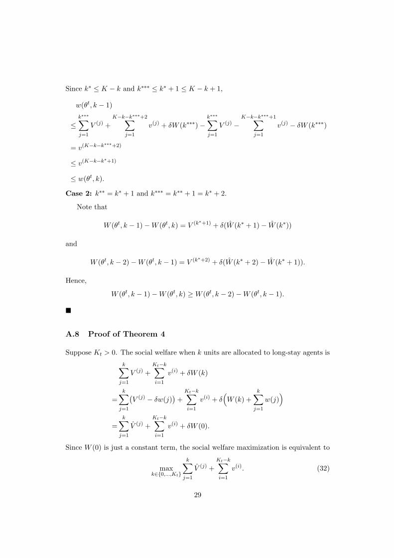
Case 2: k∗∗ = k∗ + 1 and k∗∗∗ = k∗∗ + 1 = k∗ + 2.
Note that
W (θt, k − 1) − W (θt, k) = V (k∗+1) + δ(W (k∗ + 1) − W (k∗))
and
W (θt, k − 2) − W (θt, k − 1) = V (k∗+2) + δ(W (k∗ + 2) − W (k∗ + 1)).
Hence,
W (θt, k − 1) − W (θt, k) ≥ W (θt, k − 2) − W (θt, k − 1).
¥
A.8 Proof of Theorem 4
Suppose Kt > 0. The social welfare when k units are allocated to long-stay agents is
k∑j=1
V (j) +Kt−k∑i=1
v(i) + δW (k)
=k∑
j=1
(V (j) − δw(j)
)+
Kt−k∑i=1
v(i) + δ(W (k) +
k∑j=1
w(j))
=k∑
j=1
V (j) +Kt−k∑i=1
v(i) + δW (0).
Since W (0) is just a constant term, the social welfare maximization is equivalent to
maxk∈{0,...,Kt}
k∑j=1
V (j) +Kt−k∑i=1
v(i). (32)
29
By Proposition 4, w(k) is increasing in k and thus V (k) is decreasingly ordered.
Hence, the solution of (32) is simply to select the highest Kt bids from
B ≡ {v(1), v(2), . . . , V (1), V (2), . . . }.
Note that because the efficient allocation policy when agent i is excluded is
given in the same manner, the externality that agent i gives to the other agents is
determined by the highest rejected bid or the (Kt + 1)-th highest bid of B. Let k∗
and b(j) be the solution of (32) and j-th highest bid of B, respectively. Thus, k∗
units are allocated to long-stay agents and Kt −k∗ units to short-stay agents. When
a winner i is a short-stay agent, then his payment in the dynamic VCG mechanism
is b(Kt+1) = max{v(Kt−k∗+1), V (k∗+1)}. When a winner i is a long-stay agent, then
his total payment in the dynamic VCG mechanism is V (k∗+1) if b(Kt+1) = V (k∗+1).
If b(Kt+1) = v(Kt−k∗+1), the total payment is v(Kt−k∗+1) + w(k∗). ¥
References
[1] Athey, S., and I. Segal (2013), “An Efficient Dynamic Mechanism,” Economet-
rica, 81, 2463-2485.
[2] Bikhchandani, S., S. Chatterji, R. Lavi, A. Mu’alem, N. Nisan, and A. Sen
(2006), “Weak Monotonicity Characterizes Deterministic Dominant-Strategy
Implementation,” Econometrica, 74, 1109-1132.
[3] Bergemann, D., and M. Said (2011), “Dynamic Auctions: A Survey,” Wiley
Encyclopedia of Operations Research and Management Science.
[4] Bergemann, D., and J. Valimaki (2010), “The Dynamic Pivot Mechanism,”
Econometrica, 78, 771-789.
[5] Board, S., and A. Skrzypacz (2010), “Revenue Management with Forward-
Looking Buyers,” Unpublished manuscript, Stanford University.
30
[6] Dizdar, D., A. Gershkov, and B. Moldovanu (2011), “Revenue Maximization in
the Dynamic Knapsack Problem,” Theoretical Economics, 6, 157-184.
[7] Gershkov, A., and B. Moldovanu (2009), “Dynamic Revenue Maximization with
Heterogeneous Objects: A Mechanism Design Approach,” American Economic
Journal: Microeconomics, 1, 168-198.
[8] Gershkov, A., and B. Moldovanu (2010), “Efficient Sequential Assignment with
Incomplete Information,” Games and Economic Behavior, 68, 144-154.
[9] Hajiaghayi, M., R. Kleinberg, M. Mahdian, and D.C. Parkes (2005), “Online
Auctions with Re-Usable Goods,” Proceedings of the 6th ACM Conference on
Electronic Commerce (EC ‘05), 165-174.
[10] Kittsteiner, T., and B. Moldovanu (2005), “Priority Auctions and Queue Disci-
plines That Depend on Processing Time,” Management Science, 51, 236-248.
[11] Lavi, R., and N. Nisan (2000), “Competitive Analysis of Incentive Compatible
Online Auctions,” Proceedings of the 2nd Conference on Electronic Commerce
(EC ‘00), 233-241.
[12] Lehmann, D., L.I. O’Callaghan, and Y. Shoham (2002), “Truthful Revelation
in Approximately Efficient Combinatorial Auctions,” Journal of ACM, 49, 577-
602.
[13] Mierendorff, K. (2009), “Optimal Dynamic Mechanism Design with Deadlines,”
Unpublished manuscript, University of Bonn.
[14] Milgrom, P., and I. Segal (2002), “Envelope Theorems for Arbitrary Choice
Sets,” Econometrica, 70, 583-601.
[15] Myerson, R. (1981), “Optimal Auction Design,” Mathematics of Operations
Research, 6, 58-73.
[16] Pai, M., and R. Vohra (2013), “Optimal Dynamic Auctions and Simple Index
Rules,” Mathematics of Operations Research, 38, 682-697.
31

[17] Parkes, D.C. (2007), “Online Mechanisms,” in N. Nisan, T. Roughgarden, E.
Tardos, and V.V. Vazirani (eds.), Algorithmic Game Theory, Cambridge Uni-
versity Press, New York.
[18] Parkes, D.C., and S. Singh (2003), “An MDP-Based Approach to Online Mecha-
nism Design,” Proceedings of the 17th Annual Conference on Neural Information
Processing Systems (NIPS ‘03), 791-798.
[19] Pavan, A., I. Segal, and J. Toikka (2014), “Dynamic Mechanism Design: A
Myersonian Approach,” Econometrica, 82, 601-653.
[20] Porter, R. (2004), “Mechanism Design for Online Real-Time Scheduling,” Pro-
ceedings of the 5th ACM Conference on Electronic Commerce (EC ‘04), 61-70.
[21] Riley, J., and W. Samuelson (1981), “Optimal Auctions,” American Economic
Review, 71, 381-392.
[22] Said, M. (2012), “Auctions with Dynamic Populations: Efficiency and Revenue
Maximization,” Journal of Economic Theory, 147, 2419-2438.
[23] Vulcano, G., G. van Ryzin, and C. Maglaras (2002), “Optimal Dynamic Auc-
tions for Revenue Management,” Management Science, 48, 1388-1407.
32