www.GISman.ir

Lecture Notes in Geoinformation and Cartography Series Editors: William Cartwright, Georg Gartner, Liqiu Meng,

Michael P. Peterson

www.GISman.ir

Editors: Poh C. Lai Department of Geography The University of Hong Kong Hong Kong Special Administrative Region, China Ann S.H. Mak ERM Hong Kong Taikoo Place, Island East Hong Kong Special Administrative Region, China

ISBN 10 3-540-71317-4 Springer Berlin Heidelberg New York ISBN 13 978-3-540-71317-3 Springer Berlin Heidelberg New York ISSN 1863-2246 Library of Congress Control Number: 2007929856 This work is subject to copyright. All rights are reserved, whether the whole or part of the material is concerned, specifically the rights of translation, reprinting, reuse of illustra-tions, recitation, broadcasting, reproduction on microfilm or in any other way, and stor-age in data banks. Duplication of this publication or parts thereof is permitted only under the provisions of the German Copyright Law of September 9, 1965, in its current version, and permission for use must always be obtained from Springer-Verlag. Violations are li-able to prosecution under the German Copyright Law. Springer is a part of Springer Science+Business Media springeronline.com © Springer-Verlag Berlin Heidelberg 2007 The use of general descriptive names, registered names, trademarks, etc. in this publica-tion does not imply, even in the absence of a specific statement, that such names are ex-empt from the relevant protective laws and regulations and therefore free for general use. Cover design: deblik, Berlin Production: A. Oelschläger Typesetting: Camera-ready by the Editors Printed on acid-free paper 30/2132/AO 54321

www.GISman.ir

This publication is printed with funding support from:

COMMERCE, INDUSTRY AND TECHNOLOGY BUREAU

THE GOVERNMENT OF THE HONG KONG

SPECIAL ADMINISTRATIVE REGION

Disclaimer:

Any opinions, findings, conclusions or recommendations expressed in this material / any

event organized under this Project do not reflect the views of the Government of the Hong

Kong Special Administrative Region or the Vetting Committee for the Professional Ser

vices Development Assistance Scheme.

www.GISman.ir

V

Preface

“As the world becomes more integrated through the trade of goods

and services and capital flows, it has become easier for diseases to

spread through states, over borders and across oceans — and to do

serious damage to vulnerable human and animal populations.” American RadioWorks and NPR News, 2001

The global cost of communicable diseases is expected to rise. SARS has

put the world on alert. We have now Avian Flu on the watch. Recognizing

the global nature of threats posed by new and re-emerging infectious dis-

eases and the fact that many recent occurrences originated in the Asia Pa-

cific regions, there has been an increased interest in learning and knowing

about disease surveillance and monitoring progresses made in these re-

gions. Such knowledge and awareness is necessary to reduce conflict, dis-

comfort, tension and uneasiness in future negotiations and global coopera-

tion.

Many people are talking about the GIS and public and environmental

health. The way we make public policies on health and environmental mat-

ters is changing, and there is little doubt that GIS provides powerful tools

for visualizing and linking data in public health surveillance. This book is

a result of the International Conference in GIS and Health held on 27-29

June 2006 in Hong Kong. The selected chapters are organized into four

themes: GIS Informatics; Human and Environmental Factors; Disease

modeling; and Public health, population health technologies, and surveil-

lance.

As evident from the chapters, the main problem in GIS-based epidemi-

ological studies is the availability of reliable exposure data. There is also a

huge problem of showing adequate responsibility and ability to meet pub-

lic concerns, such as protection on privacy and quick response systems.

There has been some works done in search of the right approach in bring-

ing together and reconciling market and public interests. Talking to each

other and sharing critical information are getting increasingly important.

Much work remains to be done to improve the GIS-based epidemiologic

methods into tools for fully developed analytical studies and, particularly,

the need to identify standard interfaces and infrastructures for the global

disease reporting system.

January 2007 Poh C. Lai

Ann S.H. Mak

www.GISman.ir

VI

International Conference in GIS and Health 2006

Geospatial Research and Application Frontiers in

Environmental and Public Health Systems 1

Conference Chair Poh C. Lai, University of Hong Kong, China

Program Committee International Members

Chuleeporn Jiraphongsa, Ministry of Public Health, Thailand

Nina Lam, Louisiana State University, USA

Feng Lu, Chinese Academy of Sciences, China

Augusto Pinto, World Health Organization, France

Jan Rigby, University of Sheffield, United Kingdom

Pratap Singhasivanon, University of Mahidol, Thailand

Chris Skelly, Brunel University, United Kingdom

Local Members

Ping Kwong Au Yeung, Lands Department

Lorraine Chu, Mappa Systems Limited

Tung Fung, Chinese University of Hong Kong

Tai Hing Lam, University of Hong Kong

Hui Lin, Chinese University of Hong Kong

Christopher Hoar, NGIS China Limited

S.V. Lo, Health Welfare and Food Bureau

Ann Mak, ERM Company Limited

Stanley Ng, MapAsia Company Limited

Wenzhong Shi, Hong Kong Polytechnic University

Winnie Tang, ESRI China (Hong Kong) Limited

Raymond Wong, Intergraph Hong Kong

Anthony Gar-On Yeh, University of Hong Kong

Qiming Zhou, Hong Kong Baptist University

Executive Committee Kawin K.W. Chan, University of Hong Kong

Richard K.H. Kwong, University of Hong Kong

Poh C. Lai, University of Hong Kong

Sharon T.S. Leung, NGIS China Limited

Feng Lu, Chinese Academy of Sciences

Ann S.H. Mak, ERM Company Limited

Franklin F.M. So, Experian Limited

Andrew S.F. Tong, University of Hong Kong

1 The conference was a joint event held in June 2006 and jointly organized by the Department of

Geography at the University of Hong Kong and the State Key Laboratory of Resources and

Environmental Information Systems of the Chinese Academy of Sciences. It was supported by the

Croucher Foundation and the Professional Services Development Assistance Scheme of the

Commerce, Industry and Technology Bureau of the Government of Hong Kong.

www.GISman.ir

VII

Table of Contents

GIS Informatics ........................................................................................3

Exploratory Spatial Analysis Methods in Cancer Prevention and Con-

trol

Gerard Rushton .................................................................................3

Environmental Risk Factor Diagnosis for Epidemics

Jin-feng Wang....................................................................................3

A Study on Spatial Decision Support Systems for Epidemic Disease

Prevention Based on ArcGIS

Kun Yang, Shung-yun Peng, Quan-li Xu and Yan-bo Cao ................3

Development of a Cross-Domain Web-based GIS Platform to Support

Surveillance and Control of Communicable Diseases

Cheong-wai Tsoi................................................................................3

A GIS Application for Modeling Accessibility to Health Care Centers

in Jeddah, Saudi Arabia

Abdulkader Murad.............................................................................3

Human and Environmental Factors ...................................................3

Applying GIS in Physical Activity Research: Community ‘Walkability’

and Walking Behaviors

Ester Cerin, Eva Leslie, Neville Owen and Adrian Bauman .............3

Objectively Assessing ‘Walkability’ of Local Communities: Using GIS

to Identify the Relevant Environmental Attributes

Eva Leslie, Ester Cerin, Lorinne duToit, Neville Owen and Adrian

Bauman..............................................................................................3

Developing Habitat-suitability Maps of Invasive Ragweed (Ambrosia

artemisiifolia.L) in China Using GIS and Statistical Methods

Hao Chen, Lijun Chen and Thomas P. Albright................................3

An Evaluation of a GIS-aided Garbage Collection Service for the East-

ern District of Tainan City

Jung-hong Hong and Yue-cyuan Deng..............................................3

www.GISman.ir

VIII

A Study of Air Quality Impacts on Upper Respiratory Tract Diseases

Huey-hong Hsieh, Bing-fang Hwang, Shin-jen Cheng and Yu-ming

Wang.................................................................................................. 3

Spatial Epidemiology of Asthma in Hong Kong

Franklin F.M. So and P.C. Lai .......................................................... 3

Disease Modeling.................................................................................... 3

An Alert System for Informing Environmental Risk of Dengue Infec-

tions

Ngai Sze Wong, Chi Yan Law, Man Kwan Lee,

Shui Shan Lee and Hui Lin ................................................................ 3

GIS Initiatives in Improving the Dengue Vector Control

Mandy Y.F. Tang and Cheong-wai Tsoi............................................ 3

Socio-Demographic Determinants of Malaria in Highly Infected Rural

Areas: Regional Influential Assessment Using GIS

Devi M. Prashanthi, C.R. Ranganathan and

S. Balasubramanian .......................................................................... 3

A Study of Dengue Disease Data by GIS Software in Urban Areas of

Petaling Jaya Selatan

Mokhtar Azizi Mohd Din, Md. Ghazaly Shaaban,

Taib Norlaila and Leman Norariza ................................................... 3

A Spatial-Temporal Approach to Differentiate Epidemic Risk Patterns

Tzai-hung Wen, Neal H Lin, Katherine Chun-min Lin,

I-chun Fan, Ming-daw Su and Chwan-chuen King ........................... 3

Public health, population health technologies, surveillance ...... 3

A “Spatiotemporal Analysis of Heroin Addiction” System for Hong

Kong

Phoebe Tak-ting Pang, Phoebe Lee, Wai-yan Leung,

Shui-shan Lee and Hui Lin ................................................................ 3

A Public Health Care Information System Using GIS and GPS: A Case

Study of Shiggaon

Ashok Hanjagi, Priya Srihari and A.S. Rayamane............................ 3

www.GISman.ir

IX

GIS and Health Information Provision in Post-Tsunami Nanggroe Aceh

Darussalam

Paul Harris and Dylan Shaw ............................................................3

Estimating Population Size Using Spatial Analysis Methods

A. Pinto, V. Brown, K.W. Chan, I.F. Chavez,

S. Chupraphawan, R.F. Grais, P.C. Lai, S.H. Mak,

J.E. Rigby and P. Singhasivanon.......................................................3

Avian Influenza Outbreaks of Poultry in High Risk Areas of Thailand,

June-December 2005

K. Chanachai, T. Parakgamawongsa, W. Kongkaew, S.

Chotiprasartinthara and C. Jiraphongsa ..........................................3

Contact Information and Author Index .....................................298

Subject Index...............................................................................307

www.GISman.ir

Exploratory Spatial Analysis Methods in Cancer

Prevention and Control

Gerard Rushton

The University of Iowa

Abstract: Improved geocoding practices and population coverage of can-

cer incidence records, together with linkages to other administrative record

systems, permit the development of new methods of exploratory spatial

analysis. We illustrate these developments with results from a GIS-based

workbench developed by faculty and students at the University of Iowa.

The system accesses records from the Iowa Cancer Registry. In using these

methods, the privacy of individuals is protected while still permitting re-

sults to be available for small geographic areas. Geographic masking tech-

niques are illustrated as are kernel density estimation methods used in the

context of Monte Carlo simulations of spatial patterns of selected cancer

burdens of breast, colorectal and prostate cancer in Iowa.

Keywords: cancer prevention and control, exploratory spatial analysis

1 The need for maps in cancer prevention and control

The theme of this chapter is the design of cancer maps for cancer control

and prevention activities. Abed et al. (2000) describe a framework for de-

veloping knowledge for making decisions for comprehensive cancer con-

trol and prevention. The decisions these authors have in mind involve local

communities setting objectives, planning strategies, implementing them,

and finally, determining improvements in health achieved by their activi-

ties. Each of these steps is explicitly spatial: where activities are directed,

who is affected, and whose health is improved? Location is a critical part

of this framework.

As with all chronic diseases, factors that influence the burden of the dis-

ease on any population include the behaviors of people, characteristics of

environments, and availability and accessibility of health screenings and

treatments. Objectives to improve population health, therefore, must iden-

www.GISman.ir

Exploratory Spatial Analysis Methods in Cancer Prevention and Control 3

tify spatial differences in these factors and must address strategies to

change them in ways that will lead to improved health outcomes. Cancer

maps play an important role in this process. Particularly geographic as-

pects of these tasks are:

Spatial allocation of resources;

Identification of areas with higher than expected incidence rates

(disease clusters);

Optimal location of services.

All three tasks require that the maps of the cancer burdens should cap-

ture any special demographic characteristics of local populations so that

actions for control and prevention relate to population characteristics.

None of these tasks should use cancer rates adjusted to standard population

characteristics. Yet, these are precisely the characteristics of many cancer

maps—see, for example, Pickle et al. 1996; Devesa et al. 1999.

1.1 The limitations of cancer mortality maps

In the short history of mapping cancer, most attention has been given to

mapping cancer mortality; for most countries, cancer mortality data are

collected routinely.

Since the geocode on a typical death certificate is some politically rec-

ognized area—often, in the United States a county—data is available for

counties and most maps use counties or aggregates of counties, (Devesa et

al. 1999). Mortality maps, however, are not so useful for planning control

and prevention interventions because spatial variations in mortality rates

can be due to differences in behaviors, in the environment or in local

health system characteristics. Yet, untangling risks due to differences in

these three factors is precisely what is required before plans to reduce can-

cer burdens can be established. With the development of cancer registries,

however, data is available that allows attempts to be made to separate these

influences and to develop interventions that will optimally reduce rates.

Cancer maps have a vital role to play by mapping these factors, in addition

to mortality.

1.2 The potential contribution of cancer registry data

There are two ways in which cancer registry data can be used for making

cancer maps. They can be used to break down the burden of cancer on lo-

cal populations into component parts. Assumed here is that the cancer reg-

istry is population-based; i.e. it accounts for all cases of cancer in a defined

population. Although it may rely on health care facilities for much of its

www.GISman.ir

4 Gerard Rushton

data, it must not be facility based. In most cases, registries are area-based

and track down incidences of cancer in its defined population wherever

they are diagnosed and treated. The components of interest are first con-

firmed diagnoses of cancer; the stage of the disease at the time of first di-

agnosis; the first course of treatment, survival rate, and mortality rate.

Other components of cancer are screening rates and treatment rates. Data

availability for these components often depends on the comprehensiveness

of the health information available for the defined population (see Arm-

strong 1992).

1.3 The role of exploratory spatial analysis

In “exploratory spatial analysis” of cancer, geographic scale and pattern

are explored. Each cancer map represents a decision to focus on a defined

geographic scale and specific patterns may be revealed—or concealed—by

the scale chosen. Figure 1 illustrates this principle using three infant mor-

tality maps of one county in central Iowa. Approximately 20,000 births

and 190 infant deaths occurred in this county in the four year period from

1989 through 1992. After geocoding each birth and death to its residential

address, the three maps on the right of Figure 1 show the pattern at the

scales captured by three, commonly used, administrative areas. A property

of these maps is that the variability of the infant mortality rates depends on

the size of the areas mapped. The rate for Zipcodes varies from 0 to 20

deaths per thousand births; for census tracts the rate varies from 0 to 36

and for census block groups the rate varies from 0 to 72. The legends for

each map—not shown here—must necessarily be adjusted to accommo-

date these different variances. The sensitivity of the patterns of infant mor-

tality to scale are clear on the left where geographic scales of the three

maps are formally defined as spatial filters of 1.2, 0.8, and 0.4 miles re-

spectively—applied in each case to a 0.4 mile grid from which the density

estimates were made (see Bithell 1990; Rushton and Lolonis 1996). Again,

on the left, patterns are different and depend on scale. We can conclude

that patterns depend on scale and actions based on patterns should consider

the scales at which the patterns were derived and ask whether the actions

contemplated are reliably based on the data that supported them.

www.GISman.ir

Exploratory Spatial Analysis Methods in Cancer Prevention and Control 5

Fig. 1. Infant mortality rates (deaths per 1000 births) at three different spatial

scales and their approximate counterparts using census administrative areas (leg-

end for maps on the right is not shown)

The ability to control the spatial basis of support for cancer rates is the

key idea that geographic information systems bring to the task of providing

decision support for cancer prevention and control. A key question we ask

is at what geographic scale do significant differences in cancer incidence

rates or other measures of cancer exist in any region of interest? A reason

for asking this question is so that we can decide the scale at which inter-

ventions should be planned. Logical though this question may appear, it

has not been the question that has driven the rather large literature of spa-

tial analysis of cancer. Traditionally, cancer maps were based on pre-

defined political or administrative units for which cancer data was col-

lected. Starting with regions already defined we made maps and then asked

“do we see a pattern.” Such a strategy pre-supposes that spatial variations

that occur within the regions mapped do not exist or, if present, are not

relevant or important. With GIS, however, we start with geocoded data—at

the level of points or small areas—and then we ask “at what geographic

scale do we want to view this pattern?” Thus, it is the much smaller lit-

erature of spatial analysis of cancer based on data manipulated in a GIS

that is the literature most relevant to cancer control and prevention. Cancer

maps for this purpose employ density estimation methods. Unlike tradi-

tional cancer maps that show cancer statistics based on spatial units of dif-

www.GISman.ir

6 Gerard Rushton

ferent sizes, shapes and populations that conceal scale dependent patterns,

density estimation techniques are designed to control the spatial basis of

support for the spatial pattern of any statistic of interest. These are made

possible by developments in the availability of geospatial data, geocoding

techniques, and methods of spatial analysis that allow the opportunity to

control the size, shapes and population characteristics for the spatial units

for which statistics are computed.

1.4 Mapping cancer burdens

The first measure of the cancer burden on a population is the rate of inci-

dence of any particular cancer type adjusted for age and sex of the local

population. The first choice to be made is between direct and indirect rate

adjustment methods. Direct adjustment of rates is made when rates are to

be compared from one area to another to note the rate burden on the popu-

lation. In such a situation the question being asked is the hypothetical

question “if the age-sex structure of the local population was the same as a

standard population, what would the overall cancer incidence rate be?

These rates are made by multiplying locally observed age-sex defined can-

cer rates by a common set of weights that sum to one that describe national

population characteristics, (see Pickle and White 1995). Indirect adjust-

ment of rates are made when the question being asked is “if the local popu-

lation were to have cancer incidences at the same rates as a standard popu-

lation, how much more or less does cancer occur there than in the standard

population.” Indirectly adjusted rates are best used when resources are to

be allocated to areas based on the impact of the rates on the population of

the local area—see Kleinman 1977. The second choice of cancer burden is

about the proportion of diagnosed cancer cases that are late stage at the

time of their first diagnosis. This can be measured as the proportion of in-

cidences observed in a population that are late stage, or, can be measured

as the number in a population adjusted for its age and sex characteristics.

The third choice is mortality rates. Illustrations of the different kinds of

maps of these three cancer burdens for the Iowa population between 1998

and 2002 can be seen at Beyer et al. 2006. All maps are indirectly age-

gender adjusted using national rates of cancer with the rates defined as ac-

tual observed number of cancers in the spatial filter area divided by the

number expected given the demographic characteristics of people in the

filter area. Rates defined in this way reflect the demographic characteris-

tics of the local area. Statistically they are more robust than directly age-

gender adjusted rates because they are made by multiplying national rates

that are stable by populations in the filter areas which are also stable. The

www.GISman.ir

Exploratory Spatial Analysis Methods in Cancer Prevention and Control 7

geographic detail in the indirectly adjusted rate maps is far superior to the

geographic detail possible in directly age-sex adjusted maps.

I illustrate the control of scale with design of a map of late stage colo-

rectal cancer rates in Iowa for the period 1993 through 1997. The ap-

proximate population of Iowa in 2000 was 2,800,000. The number of new

incidences of colorectal cancer in Iowa for a four year period was 8,403

cases. All were geocoded either to their street address, or, in a few cases

where the street address could not be matched to the geographic base files

to the centroid of their Zip code; there are 940 Zip code areas in Iowa. Us-

ing a regular grid of four miles, we applied the “sliding window” method

of Weinstock (1981) for estimating the late-stage rate at each node of this

regular grid. For the area surrounding each node on this grid, the rate of

late stage diagnosis is the ratio of the number of late stage colorectal can-

cers to the total number of colorectal cancers within the filter area (or ker-

nel). In Figure 2 we illustrate the grid points from which the late stage co-

lorectal cancer rates were constructed. On the right, the rates are illustrated

as average values for the closest eight neighbors to each grid point, using

an inverse distance weighting algorithm. In Figure 3 we change the scale

of the patterns by using progressively larger spatial filters from ten miles

radius to fifteen miles radius. In this illustration, we are mapping the rate

with which women diagnosed with early stage breast cancer selected

breast conserving surgery (lumpectomy with radiation) rather than the

more radical surgery—mastectomy. As is to be expected on all disease rate

maps, as the geographic scale of the map decreases (larger spatial filters),

details in the pattern—many of which are spurious because the rates are

based on small numbers—drop out and a more persistent regional pattern

emerges which is best seen on the fifteen mile filter map. The named

places on these maps had radiation facilities at the time of this data—early

1990s.

Fig. 2. Late stage colorectal cancer (number late stage per thousand cases of colo-

rectal cancer diagnosed) interpolated from computed values on the regular grid

(left)

www.GISman.ir

8 Gerard Rushton

Fig. 3. Number of women selecting lumpectomy with radiation per 1000 cases of

localized breast cancer, Iowa, 1991-1996; map on the left used 10 mile spatial fil-

ter; map on the right used 15 mile filter

The maps illustrate the tendency for women who live far from radiation

facilities to not choose this recommended surgical therapy over the tradi-

tional more radical surgery of mastectomy. Recent research confirms that

this tendency is a national phenomenon (Nattinger et al. 2001; Schroen et

al. 2005). The critical choice in such spatial filtering of disease data are se-

lection of the size of the grid and the size of the filter (Silverman 1986).

The grid size is the less important choice since providing the grid is de-

tailed enough geographically to provide the level of resolution desired in

the output, further detail in the grid will add no further value to the map.

Changing the size of the spatial filter, as illustrated in Figure 3, will affect

the pattern because the differences in rates that typically occur within the

size of the filter will be averaged or smoothed and some of the variability

in the geographic pattern will disappear.

The geographic detail of a disease density map does depend on the level

of spatial aggregation of the data used. Figure 4 illustrates late-stage colo-

rectal cancer rates for the case (left map) where input data consists of ap-

proximately 940 Zip code areas in Iowa compared with (right map) where

input data is individually geocoded cancer cases. Note that there are differ-

ences between these maps, particularly along the edges of the study area;

but the geographic patterns are also quite similar. We conclude that, at this

geographic scale—15 mile radius filters—considerable geographic detail is

preserved by using the spatially aggregated data. This is important since

geocoded data of individuals is often not made available by cancer regis-

tries in North America to researchers or to public health personnel because

of privacy laws and commitments to maintaining the confidentiality of

data records (CDC 2003; Olson et al. 2006). The improved geographic de-

tail may also be compared with Figure 5 where area-based disease maps

are based on the same data aggregated by county.

www.GISman.ir

Exploratory Spatial Analysis Methods in Cancer Prevention and Control 9

Fig. 4. Comparison of spatially filtered maps (15 mile filters) using geocoded can-

cer data at two different levels of spatial resolution. Rates of late-stage colorectal

cancer at first diagnosis 1993-1997. The map on the left is made from spatially

aggregated data which used Zipcode centroids as geocodes. The map on the right

used address-matched geocodes. The same cancer incidence data is used on both

maps.

Fig. 5. Percent of colorectal patients with late stage tumors at time of first diagno-

sis, Iowa, 1993 - 1997

1.5 Adaptive spatial filters

Further geographic detail may be achieved by adapting the size of the spa-

tial filter to the density of the disease data.

In Figure 6 the map on the left aggregates the cancer cases in order of

their distance from the grid point until at least 100 cases are found. The

map on the right of this figure shows percent late-stage colorectal cancer

rates based on a 24 mile filter. The spatially adaptive filter provides more

geographic detail in areas of high population density where the numbers of

cancer cases within any given size spatial filter area is large enough to

support a reliable estimate of the late-stage rate—Tiwari and Rushton

2004; Talbot et al. 2000. The spatial detail provided by such maps should

not be confused with the apparent geographic detail on maps that are

www.GISman.ir

10 Gerard Rushton

smoothed using rates for administrative or political entities (Kafadar

1996). Such maps use spatial smoothing functions based on centroids of

areas. Examples can be seen in two recently published cancer atlases

which superficially may appear to be similar to the mapping method pro-

posed here—Tyczynski et al. 2006; Pukkala et al. 1987. In these atlases,

rates are computed for political areas (counties in Ohio; municipal areas in

Finland)—first-level data smoothing--and then the smoothed cancer rate

surface is produced by a floating spatial filter producing a weighted aver-

age of the rates in surrounding counties—second-level data smoothing.

This double smoothing of data and then rates, we believe, should be

avoided. In kernel density estimation the data for numerator and denomi-

nator are collected for the spatially adaptive area and then the rate is com-

puted and attributed to the grid point from which the kernel is measured.

This method for controlling the change of support (see Haining 2003, p

129) is theoretically more valid than the gross spatial smoothing functions

so commonly used. Spatial interpolations are made only locally; that is, be-

tween closely spaced grid points.

Fig. 6. Adaptive spatial filter--left map uses closest 100 cases to define the filter

area from each grid point on a three mile grid; right uses a 24 mile filter area.

Number of late stage colorectal cancer cases per thousand cases at first diagnosis,

Iowa, 1993 – 1997

1.6 Adjusting for rate variability due to small numbers

The issue of reliability of rates is important. With traditional spatial den-

sity maps that use fixed size spatial filters, some local rates are based on a

large amount of information while other local rates are based on little in-

formation. A Monte Carlo procedure can be used to evaluate the statistical

significance of rates observed at any grid point. For this procedure we use

random re-labeling of the known cancer locations so that the total number

of late-stage cases in the study area is equal to the observed number of

such cases. Thus the null hypothesis being tested is that the rate of late-

www.GISman.ir

Exploratory Spatial Analysis Methods in Cancer Prevention and Control 11

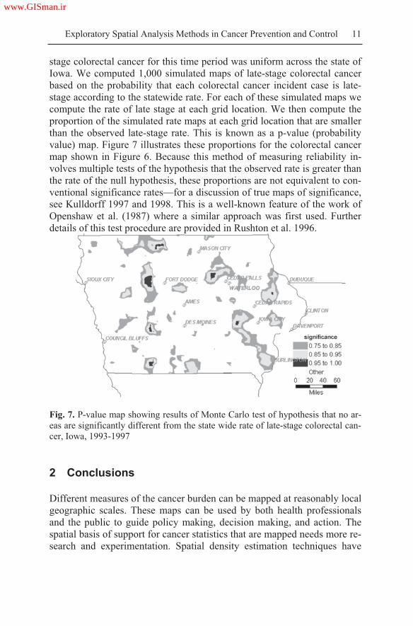
stage colorectal cancer for this time period was uniform across the state of

Iowa. We computed 1,000 simulated maps of late-stage colorectal cancer

based on the probability that each colorectal cancer incident case is late-

stage according to the statewide rate. For each of these simulated maps we

compute the rate of late stage at each grid location. We then compute the

proportion of the simulated rate maps at each grid location that are smaller

than the observed late-stage rate. This is known as a p-value (probability

value) map. Figure 7 illustrates these proportions for the colorectal cancer

map shown in Figure 6. Because this method of measuring reliability in-

volves multiple tests of the hypothesis that the observed rate is greater than

the rate of the null hypothesis, these proportions are not equivalent to con-

ventional significance rates—for a discussion of true maps of significance,

see Kulldorff 1997 and 1998. This is a well-known feature of the work of

Openshaw et al. (1987) where a similar approach was first used. Further

details of this test procedure are provided in Rushton et al. 1996.

Fig. 7. P-value map showing results of Monte Carlo test of hypothesis that no ar-

eas are significantly different from the state wide rate of late-stage colorectal can-

cer, Iowa, 1993-1997

2 Conclusions

Different measures of the cancer burden can be mapped at reasonably local

geographic scales. These maps can be used by both health professionals

and the public to guide policy making, decision making, and action. The

spatial basis of support for cancer statistics that are mapped needs more re-

search and experimentation. Spatial density estimation techniques have

www.GISman.ir

12 Gerard Rushton

been comparatively neglected in favor of inferior spatial analysis ap-

proaches that have focused on given, often inappropriate, spatial units. The

drawbacks of current mapping approaches are well-known. Rates for areas

with different population sizes differ in their reliability and many statistical

methods and spatial smoothing methods are used to compensate and adjust

for these problems. These mapping approaches do not convey clearly the

geography of the cancer burden to local communities in a form that satis-

fies the needs of the public. Better methods exist but they have not been

used with currently available geo-spatial population data and geocoded

cancer registry data largely because software to make such maps is not

available for general registry use. There are three essential properties of

more useful mapping methods:

1. Rates mapped should be based on control of the population basis that

supports them;

2. The spatial basis of this population support will typically vary in size of

area so that the geographic detail that can be validly observed will typi-

cally vary across the map;

3. The user of a cancer map should be able, for any location on the map,

know the size of the area and the size of the population that supports the

rate as well as full details of the rates mapped consistent with full pri-

vacy protection of the cancer data.

No currently available cancer map has these three essential properties

and no software tool exists to produce such a map.

An outline of the directions for research in this area can be made, based

on three principles that we accept to be true:

The deficiencies of current area-based methods for representing the spa-

tial patterns of disease will increasingly be recognized and demands for

more useful representations will grow;

The availability of finely geocoded disease data will grow although ac-

cess to such data will be increasingly tightly controlled through data

sharing agreements and legal regulations, (see Rushton et al. 2006);

The availability of demographic data for very small areas will grow as

modern censuses tabulate data for flexible, GIS controlled, areas and as

algorithms are developed for more intelligent disaggregating of demo-

graphic data to custom-defined areas, (see Cai et al. 2006; Mennis

2003; Mugglin et al. 2000).

Acknowledgments

I thank Chetan Tiwari for making Figures 2, 4 and 6.

www.GISman.ir

Exploratory Spatial Analysis Methods in Cancer Prevention and Control 13

References

[1] Abed J, Reilley B, Butler MO, Kean T, Wong F, Hohman K (2000) Develop-

ing a framework for comprehensive cancer prevention and control in the

United States: an initiative of the Centers for Disease Control and Prevention.

Jn Public Health Management Practice 6(2):67-78

[2] Armstrong B (1992) The role of the cancer registry in cancer control. Cancer

Causes and Control 3:569-579

[3] Beyer K, Chen Z, Escamilla V, Rushton G (2006) Iowa Consortium for Com-

prehensive Cancer Control Cancer Maps Site. Available at

http://www.uiowa.edu/~gishlth/ICCCCMaps/

[4] Bithell JF (1990) An application of density estimation to geographical epide-

miology. Statistics in Medicine 9:691-701

[5] Cai Q, Rushton G, Bhaduri B, Bright E, Coleman P (2006) Estimating small-

area populations by age and sex using spatial interpolation and statistical in-

ference methods. Transactions in GIS 10:577-598

[6] Centers for Disease Control and Prevention (2003) HIPAA privacy rule and

public health: guidance from CDC and the US Department of Health and Hu-

man Services. Morbidity Mortality Weekly Report 52:suppl.1-20

[7] Devesa SS, Grauman DJ, Blot WJ, Pennello GA, Hoover RN, Fraumeni, Jr.

JF (1999) Atlas of Cancer Mortality in the United States: 1950-94. NIH Publi-

cation No. 99-4564

[8] Haining RP (2003) Spatial Data Analysis: Theory and Practice. Cambridge

University Press

[9] Kafadar K (1996) Smoothing geographical data, particularly rates of disease.

Statistics in Medicine 15:2539-2560

[10] Kleinman JC (1977) Age-adjusted mortality indices for small areas: applica-

tions to health planning. American Jn. of Public Health 67(9):834-840

[11] Kulldorff M (1997) A spatial scan statistic. Communications in Statistics—

Theory and Methods 26:1481-96

[12] Kulldorff M (1998) Statistical methods for spatial epidemiology: tests for ran-

domness. In: Gatrell AC, Loytonen M (eds) GIS and Health, Taylor & Fran-

cis, Philadelphia, pp 49-62

[13] Mennis J (2003) Generating surface models of population using dasymetric

mapping. Professional Geographer 55:31-42

[14] Mugglin AS, Carlin BP, Gelfand AE (2000) Fully model-based approaches

for spatially misaligned data. Jn. of the American Statistical Association

95:877-887

[15] Nattinger AB, Kneusel RT, Hoffmann RG, Gilligan MA (2001) Relationship

of distance from a radiotherapy facility and initial breast cancer treatment. Jn

of the National Cancer Institute 93:1344-1346

[16] Olson KL, Grannis SJ, Mandl KD (2006) Privacy protection versus cluster de-

tection in spatial epidemiology. American Jn. of Public Health 96:2002-2008

www.GISman.ir

14 Gerard Rushton

[17] Openshaw S, Charlton M, Wymer C, Craft AW (1987) A Mark I geographical

analysis machine for the automated analysis of point data sets. International

Jn. of Geographic Information Systems 1:335-358

[18] Pickle LW, Mungiole M, Jones GK, White AA (1996) Atlas of United States

Mortality. Hyattsville, Maryland: National Centre for Health Statistics

[19] Pickle LW and White AA (1995) Effects of the choice of age-adjustment

method on maps of death rates. Statistics in Medicine 14:615-627

[20] Pukkala E, Gustavsson N, Teppo L (1987) Atlas of Cancer Incidence in

Finland 1953-1982. Vol. 37. Helsinki: Cancer Society of Finland

[21] Rushton G and Lolonis P (1996) Exploratory spatial analysis of birth defect

rates in an urban population. Statistics in Medicine 15:717-726

[22] Rushton G, Krishnamurthy R, Krishnamurti D, Lolonis P, Song H (1996) The

spatial relationship between infant mortality and birth defect rates in a U.S.

City. Statistics in Medicine 15:1907-1919

[23] Schroen AT, Brenin DR, Kelly MD, Knaus WA, Slingluff Jr CL (2005) Im-

pact of patient distance to radiation therapy on mastectomy use in early-stage

breast cancer patients. Jn of Clinical Oncology 23:7074-7080

[24] Silverman BW (1986) Density estimation for statistics and data analysis. Boca

Raton, FL, Chapman & Hall/CRC

[25] Talbot TO, Kulldorff M, Forand SP, Haley VB (2000) Evaluation of spatial

filters to create smoothed maps of heath data. Statistics in Medicine 19:2399-

2408

[26] Tiwari C and Rushton G (2004) Using spatially adaptive filters to map late

stage colorectal cancer incidence in Iowa. In: Fisher P (ed) Developments in

spatial data handling. Springer-Verlag, pp 665-676

[27] Tyczynski JE, Pasanen K, Berkel HJ, Pukkala E (2006) Atlas of Cancer in

Ohio: Incidence & Mortality. The Cancer Prevention Institute, Columbus,

Ohio

[28] Weinstock MA (1981) A generalized scan statistic test for the detection of

clusters. International Journal of Epidemiology 10:289-293

www.GISman.ir

Environmental Risk Factor Diagnosis for

Epidemics

Jin-feng Wang

State Key Laboratory of Resources and Environmental Information Sys-

tem, Institute of Geographical Sciences and Nature Resources Research,

Chinese Academy of Sciences

Abstract: There is evidence to suggest that the rapidly changing

physical environment and modified human behaviors have disrupted the

long-term established equilibrium of the chemical composition between

human and the Earth environment. We have noticed that environmentally

related endemic is increasingly persistent in poorer areas and occuring in

rapidly developing regions. This chapter describes two models developed

respectively to diagnose the risk of environmentally related diseases and to

simulate the spatio-temporal spread of communicable diseases. In the first

model, we used birth defects to show the diagnosis of an endemic by (i)

detecting risk areas, (ii) identifying risk factors, and (iii) discriminating

interaction between these risk factors. Here, a spatial unit is considered a

pan within which multiple environmental factors are combined to exert

impacts on the human which may lead to either positive or negative health

consequences. We were able to show that a diagnosis of environmental

risks to population health discloses the locations at risks and the potential

contribution of environment factors to the disease. In the second case, we

used SARS to show the modeling of a communicable disease by (i)

inversing epidemic parameters, (ii) recognizing spatial exposure, (iii)

detecting determinants of spread, and (iv) simulating epidemic scenarios

under various environmental and control strategies. We were able to

demonstrate spatial and temporal scenarios of the disease through the

modeling of communicable epidemic spread.

Keywords: environmentally related diseases, spatio-temporal

simulation, spatio-temporal modeling

www.GISman.ir

16 Jin-feng Wang

1 Introduction

The modern society is characterized by rapidly changing physical envi-

ronment and modified human behaviors which disrupt the long-term estab-

lished equilibrium of the chemical composition between human and the

earth environment. Increasingly, we have noticed that environmentally re-

lated endemic is persistent in poor areas and occurs in rapidly developing

regions.

The causal factors and determinants of a disease are critical in its con-

trol and intervention. These factors could be in different levels, from micro

gene, physiological, chemical or biological abnormality, to the macro me-

dia or geographical environment. Such factors at different levels could ex-

ist in a cause-effect chain or separately and independently impact the hu-

man bodies and causing diseases.

A GIS coupled with spatial analysis and spatial statistics offers power-

ful tools in exploring macro patterns and factors. The macro-level exami-

nation could suggest proxies on the visible surface of some obscured micro

agents along the cause-effect chain to uncover the real and direct causes of

a disease. Spatial analysis tools are now available to explore environmen-

tally related diseases. The causal factors X could be investigated through

cases, or a response variable y in the mathematical nomenclature, such as

spatial pattern alignment between cases y and the proposed causes X; spa-

tial ANOVA of y and x; and time series of X. This chapter looks at our ef-

forts in employing spatial analysis tools in diagnosing environmental risk

factors for diseases.

2 Inversion Epidemic Parameters

We started by exploring the inversion epidemic model which is stated sim-

ply as

= g-1(Y) Eqn. (1)

where Y denotes reported cases of infections, stands for epidemic pa-

rameters, g is a mechanistic equation of the variable Y, and -1 denotes an

inverse transformation. The epidemic parameters reflect the essential fea-

tures of an epidemic which correspond either to a unique cause or is a

complete consequence of several factors.

Two approaches can be employed to derive the parameters: (i) a field

survey which needs a huge amount of data collection work, and (ii) a

www.GISman.ir

Environmental Risk Factor Diagnosis for Epidemics 17

model reversion. If the mechanistic model of a disease is known, then only

a few cases must have the parameters reverted, because we know that

Y = mechanism epidemic parameters Eqn. (2)

where denotes a combination in a broad sense between components on

both sides of the symbol. When the first two items in Eqn (2) are known,

the epidemic parameters can then be estimated.

We used the 2003 SARS data of Beijing to illustrate the philosophy

(Wang et al. 2006). A communicable disease spreads in time in a mecha-

nism described by a time varying parameter following the SEIR model:

(t) gE I RS

a

where E(t), I(t) and R(t) are respectively the number of Exposed, Infectious

and Removed individuals at time t. S denotes the population Susceptible to

the disease. I(t), the average number of contacts per infectious person, de-

pends on time because the control effort changes over time. g is the rate at

which the exposed (latent) individuals become infectious while a is the

rate at which the infectious individuals are removed (recovered or iso-

lated). The basic reproduction number for this model is given by R0 =

l(0)/a (b+c)/a and the eventual reproduction number is approximated by

R0 b/a.

We fitted the model to the case incidence data of Beijing over the pe-

riod between 19 April and 21 June in 2003 to obtain these parameter esti-

mates: a = 0.252, b = 0.008, c = 0.588, d = 0.368, e = 54 and g = 0.200.

Figure 1 shows a fitted curve for the number of infected individuals and a

fitted curve for the transmission rate showing a very rapid decline over the

period between 20 April and 30 April. The average incubation period was

1/g or about 5 days and the average infection period was 1/a or about 4

days. Our estimate of the basic reproduction number was 2.37. The even-

tual reproduction number, achieved at around 11 June, was found to be

0.1, indicating a dramatic reduction in the reproduction number. The total

size or cases of the epidemic for estimating the epidemic parameters using

the model was 2522.

The difference between the curve of the estimated infection rate and

those of similar diseases confirmed that the model can disclose, to a certain

extent, the strength of intervention if there was no abrupt change of other

factors during the epidemic.

www.GISman.ir

18 Jin-feng Wang

Fig. 1. The Beijing epidemic and its control over time

Following a similar argument for Eqn. (2), we regarded that

Estimated Y = Observed Y + Residual Eqn. (3)

Then, the residual is actually a factor which has not been included in the

mechanism model.

3 Pattern Alignment

We also employed the spatial pattern alignment model to explore envi-

ronmentally related diseases with some degree of success. The model is

simply stated as

Pattern Y = Pattern X Eqn. (4)

where Y denotes cases of an infection and X the factors.

Birth defects, defined as "any anomaly, functional or structural, that is

present in infancy or later in life (ICBDMS)", are a major cause of infant

mortality and a leading cause of disability in China. The left side of Figure

2 illustrates the neural tube birth defect (NTD) prevalence in China; the

right side of Figure 2 shows the NTD in Heshun County of the Shangxi

province, which is the location of our pilot study.

www.GISman.ir

Environmental Risk Factor Diagnosis for Epidemics 19

Fig. 2. Neural tube birth defect (NTD) prevalence in China

NTD is believed to be caused by a multitude of factors including heredi-

tary, crude and artificially polluted environment, nutritional deficiency,

and social, economic and behavioral factors (Figure 3). However, the risk

factors associated with heredity and/or environment are very difficult to

single out from our analysis. An exhaustive survey of each of the factors in

the study area is possible but too expensive and time consuming to under-

take.

We used the pattern alignment method to justify roles of the geological

environment and the genetic factor in NTD within the study area (Wu et al.

2004). The NTD ratio was calculated according to birth defect registers

from the hospital records and field investigations in villages over a four

year period in 1998-2001. The ratio was adjusted by the Bayesian model to

reduce variation in the records of a small probability event by borrowing

strengths of its neighbors (Haining 2002). The Getis G* statistics (Getis

and Ord 1992) was used to detect spatial hotspots of the ratios in different

distance scales. Two typical clustering phenomena were found present in

the study area.

www.GISman.ir

20 Jin-feng Wang

Fig. 3. Causes of birth defects

Fig. 4. Two scales of hotspots of NTD prevalence

Service BirthDefects

Crude & Artificial

Socia

l

N

etw

ork

F

oo

d

Nutrition

Gene

En

viro

nm

en

t

Oth

ers

www.GISman.ir

Environmental Risk Factor Diagnosis for Epidemics 21

The upper left display of Figure 4 unveiled spatial clusters at a distance

of around 6.5 km, which corresponded with the average distance separa-

tion of 6.31-9.17 km among villages in the Heshun County. This average

distance of social contact indicated very little mixing of inhabitants be-

tween villages further apart which would infer that hereditary might have a

role in inducing NTD within the study area.

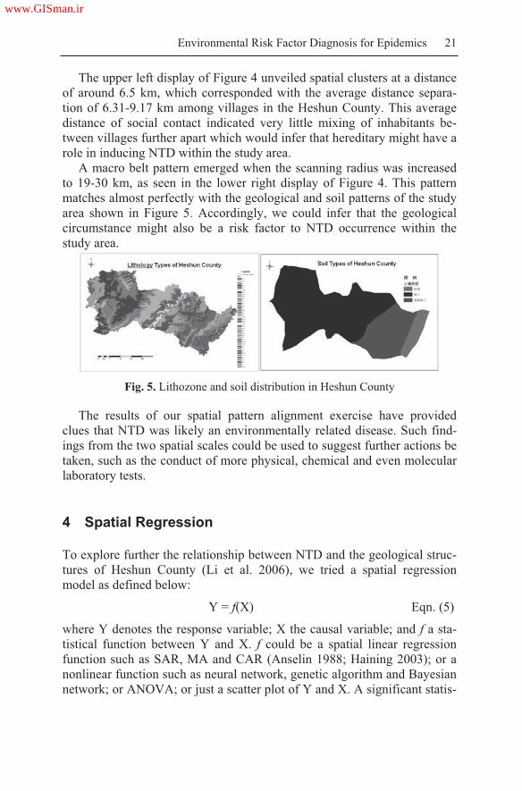
A macro belt pattern emerged when the scanning radius was increased

to 19-30 km, as seen in the lower right display of Figure 4. This pattern

matches almost perfectly with the geological and soil patterns of the study

area shown in Figure 5. Accordingly, we could infer that the geological

circumstance might also be a risk factor to NTD occurrence within the

study area.

Fig. 5. Lithozone and soil distribution in Heshun County

The results of our spatial pattern alignment exercise have provided

clues that NTD was likely an environmentally related disease. Such find-

ings from the two spatial scales could be used to suggest further actions be

taken, such as the conduct of more physical, chemical and even molecular

laboratory tests.

4 Spatial Regression

To explore further the relationship between NTD and the geological struc-

tures of Heshun County (Li et al. 2006), we tried a spatial regression

model as defined below:

Y = f(X) Eqn. (5)

where Y denotes the response variable; X the causal variable; and f a sta-

tistical function between Y and X. f could be a spatial linear regression

function such as SAR, MA and CAR (Anselin 1988; Haining 2003); or a

nonlinear function such as neural network, genetic algorithm and Bayesian

network; or ANOVA; or just a scatter plot of Y and X. A significant statis-

www.GISman.ir

22 Jin-feng Wang

tical function f would suggest that the corresponding X is the most prob-

able causal factor for the disease under examination.

The geological structure selected for the spatial regression was the loca-

tions of fault lines in Heshun County (Li et al. 2006). The study area was

divided into eight zones of buffer distance from the geological fault lines:

0–2, 2–4, 4–6, 6–8, 8–10, 10–12, 12–14, and 14–16km (Figure 6). The

NTD ratios within each of the eight buffer zones were computed and the

values graphed against the buffer distances as shown in Figure 6. The

graph discloses that the occurrence ratio of NTD birth defects was the

highest in regions at about 4 km from a fault line and the reading decreases

as the buffer distance increases. At the macro spatial scale, the geological

background showed a significant correlation with the risk of birth defects

and that people residing near the fault zones had a higher risk of having

babies with birth defects.

Fig. 6. Buffer zones of fault lines and their correlation with NTD ratio

Buffer zones of fault lines

www.GISman.ir

Environmental Risk Factor Diagnosis for Epidemics 23

A possible interpretation to the phenomena projected by Figure 6 can be

deduced from other research observations (Trique 1999; Parker and Craft

1996), such as a higher concentration of radon in the soil, water, and air

near a fault zone. The radiation emitted by radon and those of its daughter

products comprises predominantly of high linear energy transfer (LET) al-

pha radiation. Studies have indicated that the relative biological effective-

ness (RBE) of the LET alpha radiation as emitted by radon and its daugh-

ter products is 20-fold higher than those of the X-ray and gamma radiation.

A dose of the LET alpha radiation will put a fetus in the uterus in great

risks of developmental damages.

5 Time Varying Factor Detection

The disease prevalence over time can be examined with the following

model,

Z{BW(Y) | Net(X)} ~ N Eqn. (6)

where Y denotes the number of newly reported infection; X the proposed

factors of Y; and N a normal distribution. In this model, two districts are

considered connected if a linkage is the proposed channel for the transmis-

sion of Y; where a linkage can be a real geometric neighbor or a consecu-

tive district in a ranked hierarchy according to population density or other

measures. For each day within the study period, a district was coded black

(B) if a disease case was reported on that day; otherwise it was coded

white (W). Each join in the network would link two B districts or two W

districts or a pair of B and W districts. These joins were labeled as BB,

WW and BW, respectively. The observed number of BW joins was com-

pared against the expected value, and a standard normal deviation (z-

scores) was used to test its significance (Haggett 1976). A high negative

value of the z-statistics would indicate evidence of a clustering of cases in

the network and a high positive value evidence of scattering.

We investigated associations between environmental factors and SARS

by considering seven possible networks for the spread of infection among

the districts in Beijing in spring of 2003 (Meng et al. 2005). The networks

were assessed against the data using the BW join-count test. The seven

networks are listed below:

N1: Local transmission: two districts were connected if they shared a

common geographic boundary

N2: Nearest district: a district was connected to its nearest neighbor as

determined by distances between their polygon centroids

www.GISman.ir

24 Jin-feng Wang

N3: Population size: districts were ranked according to population size

and consecutive districts in this hierarchy were connected

N4: Population density: same as N3 but ranked by population density

N5: Number of doctors: same as N3 but ranked by the number of doc-

tors in a district

N6: Number of hospitals: same as N3 but ranked by the number of hos-

pitals in a district

N7: Urban-rural: Eight districts were designated as urban while the re-

mainder as rural. A rural and urban pair was connected if (i) they shared

a boundary, (ii) the urban district could be reached from the rural dis-

trict by passing through just one other rural district, or (iii) the rural dis-

trict could be reached from the urban district by passing through just

one other urban district.

For each network, we calculated the BW join-count statistics for each

day, and plotted the changes of this statistics over time.

Figure 7 shows associations between various environmental factors and

the spread of SARS infection between 27 April and 25 May 2003. The

diagrams are annotated a horizontal line indicating the threshold signifi-

cance value of the z-statistics. Figure 7(a) shows the number of cases and

the number of infected districts over time. There was a clear indication or

strong evidence in Figures 7(b) and 7(c) of transmission between the

neighboring districts towards the end of April. This local transmission con-

tinued into the first week of May but was not significant thereafter. Be-

tween 13th and 19th of May, there was clear evidence of spread between the

urban and rural areas, again a reflection of the outbreaks in the Tongzhou

district at about that time. The remaining factors showed sporadic associa-

tions with the spread of SARS, suggesting a relationship between diffusion

of infection and both the number of doctors and the population density.

www.GISman.ir

Environmental Risk Factor Diagnosis for Epidemics 25

Fig. 7. Relationship between incidence of new cases and various factors of spa-

tial spread

6 Conclusion and Discussion

The approaches to studying both environmental and communicable dis-

eases have been documented in this chapter. Four approaches have been

employed to explore relevant factors of these epidemics. Figure 8 summa-

rizes an integrative framework and prospective of these approaches to bet-

www.GISman.ir

26 Jin-feng Wang

ter understand factors leading to specific patterns of spatial spread of dis-

eases.

Fig. 8. Spatial statistics, systematic analysis and process modeling (NTD de-

notes neural tube defect; SARS denotes Severe Acute Respiratory Syndrome;

SSIR is Spatial SIR)

For environmentally related diseases, we attempted firstly to discrimi-

nate between genetic and environmental roles. The Getis G* statistics of

varying scales were used toward this end. A number of questions were of

concern: Where was the risk? Which environmental factors were responsi-

ble for the risk and what were their relative impacts? Did the factors work

independently or collectively upon a human body to lead to diseases? Our

approach considered the spatial unit as a platform within which multiple

environmental factors were combined to exert impacts on the human to re-

sult in either positive or negative health consequences. Spatial sampling

estimation, spatial regression and ANOVA were found suitable to address-

ing the above questions.

For communicable diseases, we highlighted the importance of epidemic

parameters. These parameters were essential to recognize spatial exposure,

detect determinants of spread, and simulate epidemic processes in space

and time using scenarios under various environmental and control strate-

gies. Spatial statistics and system modeling were successfully employed to

handle these issues. The different spatial statistics could be joined by

Environmental diseases (NTD) Communicable diseases (SARS)

Risk Diagnosis:

• Where is risk?

• Which factors?

• Factors ranking?

• Factors interweave?

Meta spatial statistics:

• Parameters rever-

sion

• Spatial exposure

• Spatial dynamics

• Which factors?

• Systemic analysis

Process Modeling:

• SSIR

• Process simula-

tion

Gene and/or

environment?

Environment

www.GISman.ir

Environmental Risk Factor Diagnosis for Epidemics 27

common items to produce a system fit for modeling both communicable

and environmentally related diseases.

The invention of the microscope has helped humans discover the

mechanisms of life in microscopic scales from cells to genes. The same

analogy can be used in GIS which have made visible environmental factors

related to life and linked these factors to a single or multiple groups of the

population. By the same token, spatial analysis has helped investigations

of relationships between human health and the proposed factors through

the abilities to integrate many kinds of spatially related information.

The huge amounts of data from the micro genome to the macro digital

earth have promoted the developments of bioinformatics and geoinformat-

ics respectively. Pattern alignment and correlation, spatial prediction, hot-

spot detection are current topics of research interests in both bioinformat-

ics and geoinformatics. It has been said that the two distinct disciplines

have at least a 70% overlap in the mathematics employed, including the

Bayesian inference, dynamic program, Markov chain, simulated annealing,

genetic algorithm, probability likelihood, cluster, HMM (hind markov

model), SVM (support vector machine), CA (Cella Automa), etc. (Baldi

and Brunak 1998; Haining 2003). With findings accumulated from funda-

mental research and improvements made thus far, both tools are now em-

ployable in human decision making; for example, finding petrol deposits

and searching for pathogenic genes, producing GIS products and inventing

genetic pharmacy, and building government decision support systems and

carrying out genetic therapies.

Besides sharing a common methodology and philosophy, bioinformat-

ics and geoinformatics are influencing one another. For example, GIS is

used in displaying and undertaking spatial analysis for genome studies

(Dolan 2006) and in tracking global genetic change and global climate

warming (Balanya 2006) in addition to evidence from glaciers and lake

sedimentation. The micro mechanism of a macro phenomenon is also re-

vealing; for instance, 99% of mouse genes have homologues in man or di-

verged from a common ancestor (http://www.evolutionpages.com/Mouse

genome genes.htm#Homologues). The macro phenomena also provide

clues for micro mechanisms; for instance, the two level spatial clusters of

NTD prevalence in Heshun County suggested that both hereditary and

geological factors had controlling influence of the disease in the area (Wu

et al 2004); micro pathogenic agents were found to react under both

physiological and natural environments; and the macro transmission of an

epidemic could be modeled successfully (Nakaya et al. 2005; Xu et al.

2006). The molecular epidemics and genetic epidemics have emerged to

explain macro phenomena from the micro mechanisms and the focus of

investigation on life processes has moved from a single genome analysis to

www.GISman.ir

28 Jin-feng Wang

a more integrated protein function group. The above progresses made in

bioinformatics and geoinformatics have suggested that a model can me-

chanically link micro and macro processes and an examination of the rele-

vant factors would be necessary to impart a better understanding on the

systems of life.

We highlighted three challenges in the use of spatial statistics in epi-

demics research: (1) small sample problems, (2) problems of large

amounts of data versus large amounts of variables, and (3) problems in

map comparison. Firstly, there is a high variation in the sample size of rare

diseases or diseases with short term records, which often leads to biases in

the confidence interval of estimation. Although such a variation can be re-

duced somewhat by the empirical Bayesian-adjusted technique which bor-

rows strength from the neighbors or by inserting artificial data through sto-

chastic simulations (Rushton and Lolonis 1996), we need much more

reliable theories to handle the problem. Secondly, more variables are now

available following better cooperation and coordination of the globally

connected communities (Goodchild and Haining 2004) but disease inci-

dence cases or samples have decreased because of better human controls.

There is also the dilemma of wanting local data and analyzing data accu-

rate to the individual level while having, at the same time, the ability to

compile a global statistics. We need to explore diseases with a large

amount of variables but having a few cases. This situation is contrary to

the large number theory upon which modern statistics is based, thus pre-

senting new challenges to existing statistical theories and models. Finally,

spatial patterns of some diseases change with time, and comparison be-

tween disease case patterns and those of suspected factors should reduce

the uncertainty of the hypotheses. But patterns and shapes are difficult to

describe in natural languages, which form the prerequisite for artificial in-

ference. There is here a need to explore more efficient tools for shape

analyses.

Acknowledgement

This work was supported by the National Science Foundation under Grants

#40471111 and #70571076, and by the 973 Project under Grant

#2001CB5103.

www.GISman.ir

Environmental Risk Factor Diagnosis for Epidemics 29

Reference

[1] Balanya J, Oller J, Huey R, Gilchrist G, Serra L (2006) Global Genetic

Change Tracks Global Climate Warming in Drosophila subobscura. Science

313(22): 1773-1775

[2] Baldi P and Brunak S (1998) Bioinformatics - The machine learning ap-

proach. MIT Press, Cambridge MA

[3] Dolan M, Holden C, Beard M, Bult C (2006) Genomes as geography: using

GIS technology to build interactive genome feature maps. BMC Bioinformat-

ics 7:416 (19 September 2006 )

[4] Getis A and Ord JK (1992) The analysis of spatial association by use of dis-

tance statistics. Geographical Analysis 24:189-206

[5] Goodchild M and Haining R. (2004) GIS and spatial data analysis: Converg-

ing perspectives. Papers Reg. Sci. 83, 363-385

[6] Haggett P (1976) Hybridizing alternative models of an epidemic diffusion

process. Economic Geography 52,136-146

[7] Haining R (2003) Spatial Data analysis, Theory and Practice. Cambridge

University Press

[8] Li XH, Wang JF, Liao YL, Meng B, Zheng XY (2006) A geological analysis

for the environmental cause of human birth defects based on GIS. Toxicologi-

cal & Environmental Chemistry 88(3): 551–559

[9] Meng B, Wang JF, Liu JY, Wu JL, Zhong ES (2005) Understanding the spa-

tial diffusion process of severe acute respiratory syndrome in Beijing. Public

Health 119: 1080–1087

[10] Nakaya T, Nakase K, Osaka K (2005) Spatio-temporal modeling of the HIV

epidemic in Japan based on the national HIV/AIDS surveillance. Journal of

Geographical Systems 7: 313–336

[11] Parker L and Craft AW (1996) Radon and childhood cancers. Eur. J. Cancer

32:201–204

[12] Rushton G and Lolonis P (1996) Exploratory spatial analysis of birth defect

rates in an urban population. Statistics in Medicine 15: 717-726

[13] Trique M (1999) Radon emanation and electric potential variations associated

with transient deformation near reservoir lakes. Nature 399:137–141

[14] Wang JF, McMichael AJ, Meng B, Becker NG, Han WG, Glass K, Wu JW,

Liu XH, Liu JY, Li XW (2006) Spatial dynamics of an epidemic of severe

acute respiratory syndrome in an urban area. Bulletin of the World Health Or-

ganization. In press

[15] Wu JL, Wang JF, Meng B, Chen G, Pang LH, Song XM, Zhang KL, Zhang

T, Zheng XY (2004) Exploratory spatial data analysis for the identification of

risk factors to birth defects. BMC Public Health 4:23

[16] Xu B, Gong P, Seto E., Liang S, Yang Y, Wen S, Qiu D, Gu X, Spear R

(2006) A spatial-temporal model for assessing the effects of intervillage con-

nectivity in Schistosomiasis transmission. Annals of the Association of Ameri-

can Geographers 96(1): 31–46

www.GISman.ir

A Study on Spatial Decision Support Systems for

Epidemic Disease Prevention Based on ArcGIS

Kun Yang, Shung-yun Peng, Quan-li Xu and Yan-bo Cao

Faculty of Tourism and Geographic Science, Yunnan Normal University,

Kunming, China.

Abstract: Having analyzed the current status and existing problems of

Geographic Information Systems (GIS) applications in epidemiology, this

chapter proposes a method to establish a spatial decision support system

(SDSS) for the prevention of epidemic diseases by integrating the COM

GIS, spatial database, gps, remote sensing, and communication technolo-

gies, as well as ASP and ActiveX software development technologies. One

important issue in constructing the SDSS for epidemic disease prevention

concerns the incorporation of epidemic spread models in a GIS. The chap-

ter begins with a description of the capabilities of GIS in epidemic preven-

tion. Some established models of an epidemic spread are studied to extract

essential computational parameters. A technical schema is then proposed

to integrate epidemic models using a GIS and relevant geospatial tech-

nologies. The GIS and modeling platforms share a common spatial data-

base and the modeled results can be visualized spatially by desktop and

Web clients. A complete solution for establishing the SDSS for epidemic

disease prevention based on the model integrating methods and the Ar-

cGIS software is suggested in this chapter. The proposed SDSS comprises

several sub-systems: data acquisition, network communication, model in-

tegration, epidemic disease information spatial database, epidemic disease

information query and statistical analysis, epidemic disease dynamic sur-

veillance, epidemic disease information spatial analysis and decision sup-

port, as well as epidemic disease information publishing based on the Web

GIS technology. The design process and sample VC and VB programming

codes of the epidemic case precaution are used as an example to illustrate

the basic principles and methods of the system development that integrates

GIS functions with models of epidemic spread. A case study of AIDS in

the Yunnan Province of China exemplifies the systems spatial analytical

functions through its spatial database access and statistical analysis tools.

Keywords: epidemic disease spread models, model integration methods,

epidemic spatial database, spatial decision support systems

www.GISman.ir

Spatial Decision Support Systems for Epidemic Disease Prevention 31

1 Introduction

Epidemic diseases (such as SARS, AIDS and bird flu) are highly conta-

gious and pose a threat to human life, hindering social and economic de-

velopment and progress. Outbreaks and uncontrollable spread of an epi-

demic disease can cause serious public health problems of social and

political significance. Spatial information systems containing spatial and

temporal data on epidemic diseases and their application models can help a

government and its public health institutions to realize disease monitoring

and surveillance. Such a system has been known to uncover relations be-

tween a disease and its geographical environment, as well as to offer deci-

sion support in preventing an epidemic from spreading [11].

The first application of spatial epidemiology dates back to 1854 when

John Snow succeeded in locating the origin of cholera in London by link-

ing the disease with water pumps on a map at the local scale. Further de-

velopment of the spatial information technologies in public health took

place in the developed countries. These research developments have re-

sulted in a range of tools and methodological approaches, including

mathematical models of epidemic disease spread, integration of epidemic

spread models in GIS, spatial and temporal epidemic analysis modeling,

and preventive what-if scenarios. The scientific and technological

achievements offer essential backgrounds and foundations for this re-

search.

The unrelenting problems about the use of spatial information technolo-

gies in epidemiology are none other than insufficient data, deficient spatial

and temporal modeling procedures and inadequate integration of epidemic

models in GIS. Likewise, the problems of spatial epidemic disease data-

bases and the integration of epidemic disease spread models in a GIS are

the key issues to resolve in the construction of an SDSS for epidemic dis-

ease prevention. Using the ArcGIS software platform, a method is pro-

posed here for the development of the SDSS.

2 Epidemic Spread Models and Integrated Applications in GIS

2.1 Roles of the GIS in Epidemic Disease Prevention

GIS is a technology to deal with spatial and temporal data. It offers visu-

alization and spatial analysis tools to monitor the spread of an epidemic

disease. It is suitable for the development of a disease tracking and preven-

www.GISman.ir

32 Kun Yang, Shung-yun Peng, Quan-li Xu and Yan-bo Cao

tion system given its spatial data acquisition and processing abilities, as

well as its powerful spatial analysis functions.

The origin and subsequent spread of epidemic diseases have a close re-

lation with time and geographic locations. If disease data are captured in

space/location and time and they contain essential disease attributes, the

spatial distribution and temporal characteristics of the disease spread may

be monitored and visualized for probable intervention. With the availabil-

ity of disease spread models, the contagious process may be dynamically

simulated and visualized in two or three dimensional spatial scales. Conse-

quently, high-risk population groups may be identified and visually located

while the spatial distributional patterns and spreading behaviors of a dis-

ease may be uncovered. More effective prevention decisions may be made

by the government and public health institutions through better allocation

of medical resources by using the network analysis models of a GIS.

The use of GIS technologies in epidemic disease modeling and preven-

tion will not only promote mutual developments in epidemiology and geo-

graphic information science, but will also promote the formation and de-

velopment of spatial epidemiology, which has significant theoretical and

practical values given an increased global concern over communicable dis-

eases[13].

2.2 Mathematical Models on Epidemic Spread

Several popular models on epidemic disease spread include the SIS/SIR,

Smallworld Network Dynamic and Cellular-Automata models, among

which the SIS/SIR models are the most popular and mature epidemic mod-

els. Grassberger presented the SIR model to describe spreading behaviors

of an epidemic over a network[3] and proposed that the network based SIR

model may be analogous to percolation issues in the network[9]. His find-

ing was later extended by Sander to deal with more general situations[4].

In the following equation, if and are not the same at every

node on the network but fit for ( )iP

and ( )rP

distribution, Newman

has proved that the network based SIR model is equal to a percolation is-

sue[5] with the bond occupying rate of

01 ( ) ( )i rT P P e d d

………….. Eqn. 1

Therefore, the analytical solution of a network based SIR model may be

obtained if the topological structure is given and the deterministic ( )iP

and( )rP

distribution can be confirmed.

www.GISman.ir

Spatial Decision Support Systems for Epidemic Disease Prevention 33

However, the SIR model is not suitable for patients with diseases such

as tuberculosis and gonorrhea because these patients may not be immune

from the diseases and may become susceptible to the illnesses again. For

these diseases, the SIS model described below is more appropriate:

,ds di

is i is idt dt .…………….. Eqn. 2

The SIS model is different from the SIR given that the network based SIS

model may not obtain an accurate solution. Pastor-Satorras and Vespignani

provided a very good approximate solution by using the mean field

method[6][7].

There are many more epidemic spread models for various epidemic dis-

eases besides the SIR and SIS models described above. For diseases with a

limited immunity period, the SIR model is usually used to analyze the

spreading behaviors. For diseases with latent periods, the concepts of la-

tent population groups must be accounted for relevant estimations[2].

2.3 Integrating Epidemic Models in a GIS

The integration of application models in a GIS has been a research hot spot

since 1980s. Broadly speaking, three technical aspects must be dealt within

model integration. These include data management (i.e. acquisition, proc-

essing, storage and organization), model computing (i.e. application analy-

sis), and model output (i.e. expressing simulated results in graphic or car-

tographic displays). Model integration in practice must consider specific

application requirements because of different application settings. The

COM based integration method has become a popular and feasible choice

of model integration in SDSS development because of its flexibility, al-

though the model base scheme is more ideal for model management and

intelligent processing[3].

Looking at parameters in the equations of epidemic models, it is appar-

ent that these parameters are not directly related to geographical locations

which mean problems for model integration with a GIS. The COM integra-

tion method is thus adopted, as explained below and illustrated in Figure 1.

In the modeling of data management, not only are high resolution remote

sensing images and vector graphic data effectively stored but also the input

parameters of the epidemic models stored as attributes in the spatial data-

base. The spatial data management technology of GIS can offer a better

data interface for model computing in this case. The mathematical model

can be integrated into a GIS with COM and the model computing results

stored in the same epidemic spatial database with reference to geographic

www.GISman.ir

34 Kun Yang, Shung-yun Peng, Quan-li Xu and Yan-bo Cao

GIS Platform

Data Model

Visualization

Spatial Analysis

SIS

/SIR

Models

CA

Models

Epidemic Models

Sm

all-Wo

rld M

od

els

Output

Encapsulation COM/DCOM RS Platform Image Process

Statistics Forecasting Spread Trends Map/Table

Epidemic Database

locations. The simulated results may also be visualized in geographic dis-

tributional patterns.

Fig. 1. The integration framework of COM GIS with epidemic spread models

3 System Development and Implementation

3.1 System Development

The epidemic prevention SDSS involves the integration of GPS, COM

GIS, Remote Sensing, Network Communication, Spatial and Temporal

Modeling technologies, to support data of multiple scales and formats. The

proposed system should also possess the following functions: spatial data

editing and processing, spatial modeling, epidemic information querying

and publishing, epidemic dynamic surveillance and management, medical

resource allocation and facilities planning, epidemic data maintenance,

system protection, and user right management functions[8]. The software

development setting included the following components:

Techniques: COM, ASP, Web Service, XML/SOAP;

Modes: Mixed C/S and B/S;

Tools: Microsoft Visual Studio6.0;

Development Platforms

www.GISman.ir

Spatial Decision Support Systems for Epidemic Disease Prevention 35

Client Side: ESRI ArcObjects, MapObjects, ArcGIS Server

and ArcGIS Engine;

Server Side: ESRI ArcGIS Server and ArcIMS;

Application Platforms

Client Side: ArcGIS Desktop and IE Viewer as well as Ar-

cObjects, MapObjects and ArcGIS Engine Client;

Server Side: ESRI ArcIMS and ArcGIS Server;

Database: Oracle9i, SQL Server + ArcSDE

3.2 System Structure

The epidemic prevention SDSS comprises several subsystems: (i) data ac-

quisition (including GPS, GIS and Remote Sensing technologies, etc.), (ii)

network communications, (iii) model base, (iv) epidemic spatial database,

(v) epidemic information query and statistical analysis, (vi) real time epi-

demic surveillance, (vii) epidemic spatial modeling and decision support,

and (viii) epidemic spatial information publishing. The systems structure is

as shown in Figure 2[12].

The method of accessing epidemic spatial database varies according to

the kinds of epidemic spatial information. ArcSDE, a spatial data access-

ing middleware from ESRI, is used to retrieve spatial and epidemic data

for query, display and record keeping. However, Oracle Objects of the

OLE (OO4O) technology from the Oracle Corporation is more suited for

retrieving non-spatial data. The OO4O is a COM technology based API for

database connection and has a special optimized design for the Oracle Da-

tabase Systems. Through calling the COM objects and instances of class

library offered by OO4O, the client application programs may connect

seamlessly to the Oracle database, and the connection speed is faster than

that of ADO and other database connection technologies. In addition, the

database operational functions offered by the OO4O technology are also

more powerful and plentiful.

www.GISman.ir

36 Kun Yang, Shung-yun Peng, Quan-li Xu and Yan-bo Cao

Models

LAN

Epidemic Prevention

Policy, Medicine and

OA Information ….

DEM

Data acquisition and Communication

GPS Data Acquisition

Field Investigation Data

Image Data Extraction ….

Statistical Modeling

Forecasting

Spatial Modeling

Cluster Modeling

Dynamic Modeling

Tracing Modeling

Information Query and Statistics

Location Based Query

Attribute Based Query

Spatial and Temporal Statistics ….

Information Real Time Surveillance

Facility Query: Location/Allocation

High Risk Region Segregation and Query

Real Time Alarm, Display and Process-

ing....

Internet Information Publishing

Epidemic Information Publishing on Web

Statistical Query on Web

Decision Analysis Results Publishing ….

Co

mm

un

ic

at

io

n

GPRS

SM

Mobile GIS

Web GIS

Epidemic

Spatial

Database

GIS Data: Topographic, Transpor-

tation, Environment, Vegetation,

etc.

Epidemic Data: Hospital, Surveil-

lance Station, Residence, Leisure

Places, Etc.

Image Data: DOM, etc.

Systems

Administration

Sp

atial Data

Non

-Sp

atial Data

GI

S D

ec

is

io

n S

up

po

rt

P

la

tf

or

m

Spatial

and

Temporal

Modeling

Spatial Modeling and Decision Support

Spatial Spread and Temporal Epidemic

Trends

Spatial and Temporal Epidemic Forecast-

ing

Epidemic High Risk Population Tracing

….

Fig. 2. General structure of the Epidemic SDSS

3.3 Epidemic Spatial Database Construction

With regard to data requirements of the epidemic models and functional

characteristics of the decision platform, the following data types are essen-

tial: (i) graphic data (including multi-Scale Vector Map Data, GPS located

hot spot data and areas of interest extracted from high resolution images,

etc.), (ii) epidemic attribute data, and (iii) relevant social and economic

data. These data may be easily stored in an epidemic spatial database (such

as the Oracle or SQL Sever) through the use of a Spatial Database Engine

www.GISman.ir

Spatial Decision Support Systems for Epidemic Disease Prevention 37

(as in ESRI ArcSDE)[10]. Data requirements for the epidemic prevention

decision support spatial information systems are as listed in Table 1.

Table 1. A table of data requirements for the epidemic decision support spatial in-

formation systems

Data Types Data Names Scales Data Usages

Basic Maps 1 10000

or above As Display Background

Buildings1 500 to

1 10000Include Related Attributes

Geographic

Data

Roads1 500 to

1 10000

Include Road Signs and Video

Cam

Epidemic

Cases 1 10000

Epidemic Distribution and Attrib

utes

Facilities 1 500 to

1 10000

Include Administrative Jurisdic

tions, Hospitals, CDC, Etc.

Map Signs Scale Free Include Geographic and Epidemic

Thematic Map Signs

Spat

ial

Dat

a

Epidemic

Thematic

Data

Related Infor

mation

1 500 to

1 10000

Key Epidemic Sites Net Bar,

Schools, Transportation Stations,

Airports, Water Sources and

Monitoring Sites, Etc.

User Manage

mentUser Name, Password and User Rights, Etc.

Systems

Manage

ment Data Log Data Systems Access Time and Maintenance Status

Matching Ta

bleEpidemic Case Type Matching Tables

Systems

Dictionary Translation

Table

Translation Table for Items Names, Map Layer

Names, and Item Values, Etc.

Related Table Used for more related attribute information man

agement.

Non-S

pat

ial

Dat

a

Related In

formationMIS/OA Epidemic Attribute Data

3.4 Technical Implementation

The technical implementation of the system mainly concerns COM GIS

and relevant software development technologies including ArcObjects,

ArcIMS, Visual C++6.0, Visual Basic6.0, Visual InterDev6.0, ASP, Ora-

cle9i + ArcSDE8.X, Decision Analysis Models, et cetera. The COM GIS

technology plays a key role in integrating epidemic models with GIS func-

tions and making analytical results spatial and visual. The system compo-

nents and key technologies are illustrated in Figure 3.

www.GISman.ir

38 Kun Yang, Shung-yun Peng, Quan-li Xu and Yan-bo Cao

Fig. 3. System components and key technologies

It is recognized readily from Figure 3 that the professional function de-

velopment based on AO is the key technology for system implementation.

To illustrate the basic principles and methods for the system development,

the following discussions offer sample codes for a component function of

the epidemic case precaution using the VC and VB development tools.

1. Assign a name for the component function and its interface as shown in

Figure 4, which includes one attribute and two methods.

Fig. 4. An interface map of the component function on epidemic case precaution

Implementation in the VC environment.

Create an Interface Class: Add a new ATL project named

PH AO CasePrecaution to realize the above attribute and methods

through adding ATL Simple Objects.

Introduce AO component library: Introduce AO core components in

StdAfx.h with the following codes:

PH_AO_CSAEPRECAUTION

Map:LPUNKNOWN

ShowDlg ( )

Close ( )

www.GISman.ir

Spatial Decision Support Systems for Epidemic Disease Prevention 39

#im

port"D:\arcgis\arcexe83\Bin\esriCore.olb"raw_interfaces_only,raw_native_types,no_namespace,na

med_guidsexclude("OLE_HANDLE","OLE_COLOR")

Introduce OO4O class library (Oip9.tlb): Put oip9.h into the present

project class.

Call the introduced objects: according to the project, using C++ intelli-

gent pointersto call AO component interfaces OO4O access objects.

The following contains codes for executing a spatial query:

IFeatureCursorPtr _pFeatureCur; //spatial database pointers;

IFeaturePtr _pFeature; //map layer features;

IGeometryPtr _pGeometry; //feature geometric type;

//create spatial query conditions

ISpatialFilterPtr _pSpatialFilter(CLSID_SpatialFilter);

// SQL query process

While(if record is not vacant)

{

if(FAILED(_pSpatialFilter >put_WhereClause(“AJLX ‘AIDS’”)))return false;

_pFeatureCur >NextFeature(&_pFeature);

if(_pFeature NULL) break;

_pFeature >get_Shape(&_pGeometry);

_pSpatialFilter >putref_Geometry(_pGeometry);

_pSpatialFilter >put_GeometryField(GeometryFld);

_pSpatialFilter >put_SpatialRel(esriSpatialRelContains);

_pSpatialFilter

>put_SpatialRelDescription(::_com_util::ConvertStringToBSTR(_T("T********")));

//if the relation is contain

_pSpatialFilter >put_SpatialRel(esriSpatialRelRelation);

//compute the number of epidemic cases, and make precautions.

……

}

through defining the following OO4O objects may access Oracle attributes.

OraSessionPtr _OraSes; // Oracle object intelligent pointer

OraDatabasePtr _OraDB; // Oracle object intelligent pointer

OraDynasetPtr _oraDyn; // Oracle object intelligent pointer

OraFieldsPtr _OraFds; // Oracle items object intelligent pointer

//the process for connecting and operating Oracle

// COM initialization

HRESULT hr ::CoInitialize(NULL);

if(FAILED(hr)) ::CoUninitialize();

//create objects for database working space

hr _OraSes.CreateInstance("OracleInProcServer.XOraSession");

if(FAILED(hr)) return FALSE;

//open database

this >_OraDB this >_OraSes >GetOpenDatabase( Database Service Name,

Username/Password, ORADB_DEFAULT );

//start database transaction process

this >_OraSes >BeginTrans();

// executing SQL query store the results into data sets

this >_oraDyn this >_OraDB >GetCreateDynaset("select * from layername ORDER BY

LAYERINDEX",ORADB_DEFAULT,&vtMissing);

//get present items, start to operate Oracle table

_OraFds this >_OraDset >GetFields();

……

www.GISman.ir

40 Kun Yang, Shung-yun Peng, Quan-li Xu and Yan-bo Cao

2. Integrating GIS components by using VB codes.

‘create PH_AO_CASEPRECAUTION objects

Dim m_Caseprecaution As PH_AO_CASEPRECAUTIONLib.AO_CasePrecaution

‘calling PH_AO_CASEPRECAUTION attributes and methods realizing the functions

Set m_ CasePrecaution New PH_AO_CASEPRECAUTIONLib.AO_CasePrecaution

m_ CasePrecaution.Map MapControl1.Map

m_ CasePrecaution.ShowDlg

3.5 Integration of Systems Function

Besides the basic capabilities of epidemic data query and statistical analy-

sis, the epidemic SDSS offers a list of professional and advanced functions

(Table 2). These include a query function for locating medical facilities,

location and allocation modeling of medical resources, dynamic zoning of

high risk and quarantine areas, the publishing of real time surveillance in-

formation, as well as epidemic prevention spatial decision analysis func-

tions. The structural organization of functions for the epidemic SDSS is

outlined in Table 2.

The epidemic SDSS is tested using the AIDS monitoring data in the

Yunnan Province of China as a case study. Figure 5 displays results of the

statistical analyses of the data as well as spatial distributional patterns of

AIDS cases in Yunnan [14]. The systems interfaces are also illustrated in

the figure.

The epidemic SDSS offers various analytical and visualization functions

including thematic maps, statistical graphs/charts and tables. These func-

tions enable displays of the spatial distributional patterns of an epidemic

disease and, in conjunction with the integrated epidemic spread models,

may reveal the spreading tendency of the disease. The epidemic SDSS

provides information beneficial to relevant government and public health

institutions that facilitates them to make informed decisions on control and

intervention measures.

www.GISman.ir

Spatial Decision Support Systems for Epidemic Disease Prevention 41

Table 2. A chart of systems functions

Sequence Function

ClassificationFunction Descriptions

1Basic GIS

Functions

Include User Management, Data Management, Map

Operation, Map Editing, Map Query, etc.

Epidemic Case Query 2

Epidemic

Information Query Other Relevant Thematic Information Query

Epidemic Case Statistics , Spatial and Temporal

Distribution Analysis 3

Epidemic

Information

Statistics Other Relevant Information Statistics

Network Analysis

Precaution Analysis according to the Epidemic Case

Numbers

Medical Resource Location/Allocation

What if Scenarios

Epidemic Case Forecasting According to the Fore

casting Models

3D Police Information Analysis

Trend Surface Analysis

4

Epidemic

Information

Analysis

Disaster Evaluation and Recovering Planning

Analysis Results Publishing Based on Web GIS

JPG, BMP Image Output 5Decision Analysis

Results Output Print Output

Fig. 4. The system interface and results of the Epidemic SDSS illustrating AIDS

distribution in the Yunnan Province of China

www.GISman.ir

42 Kun Yang, Shung-yun Peng, Quan-li Xu and Yan-bo Cao

4 Conclusion

Modern technological developments have strengthened man’s ability to

prevent epidemic diseases to a large extent. However, the human race is

still facing problems in understanding disease spread at various spatial

scales (i.e. local, regional, and global), recognizing highly contagious dis-

eases, and effectively detecting outbreaks before they happen. This chapter

has demonstrated the values of spatial information technologies in an epi-

demic SDSS through the integration of epidemic spread models in a GIS.

The epidemic SDSS can assist the government and relevant public health

institutions manage disease data spatially and temporally such that disease

data can be correlated with environmental and social economic factors.

The overall aim is to tap benefits of spatial information technologies in de-

livering SDSS to effectively monitor and prevent disease spread.

Acknowledgement

This research is financially supported by the National Science Foundation

of China under Grant No. 30560135 and the Yunnan Provincial Science

Foundation under Grant No.2004D0032M.

Reference

[1] Grimmett GR (1989) Percolation. Berlin: Springer-Verlag

[2] Li Z and Cui H (2003) SI Models and Piecewise SI Model on SARS Forecast-

ing. Journal of Remote Sensing. 7 (5):10-14

[3] Lu G and Zhang S (2003) The Integration Principles and Methods of Geo-

graphic Information Systems. Beijing: Science Press 1~345 pp

[4] Newman M E J (2002) Spread of epidemic disease on networks. Phys Rev E,

66, 016128

[5] Pastor-Satorras R and Vespignani A (2001) Epidemic dynamics and endemic

states in complex networks. Phys Rev E, 63, 066117

[6] Pastor-Satorras R and Vespignani A (2001) Epidemic spreading in scale-free

networks. Phys Rev Lett, 86, 3200-3203

[7] Pastor-Satorras R and Vespignani A (2003) Epidemics and immunization in

scale-free networks. In Bornholdt S, Schuster HG (eds.) Handbook of graph

and networks. Berlin: Wiley-VCH

[8] Qi X and Lu F (2004) GIS Application and Development in Epidemiology.

Chinese Journal of Epidemiology. 25(11):83-85

www.GISman.ir

Spatial Decision Support Systems for Epidemic Disease Prevention 43

[9] Sander LM and Warren CP (2002) Percolation on disordered networks as a

model for epidemics. Math Biosci, 180:293-305

[10] Wen L and Xu D (2004) The Construction of Malaria Precaution Systems

Based on GIS. Chinese Journal of Public Health 20(5):118-119

[11] Xu Z and Z. (2004) GIS Applications in Epidemiology. Chinese Journal of

Public Health. 20(8):130-132

[12] Zhong K. and H. (2004) The Design and Implementation of Epidemic Disease

Emergency Response Decision Support Systems Based on GIS/GSM. Journal

of Surveying and Mapping Science. 2004.1:36-39

[13] Zhou Y. and T. (2003) The Mathematical Models for SARS Spread Forecast-

ing. Chinese Journal of Engineering Mathematics. 20(S2):33-38

[14] Lu L and Jia M. (2005) 1989-2004 AIDS Epidemic Analysis of Yunnan Prov-

ince, Chinese Journal of AIDS & STD, 2005.9:178-182

www.GISman.ir

Development of a Cross-Domain Web-based GIS

Platform to Support Surveillance and Control of

Communicable Diseases

Cheong-wai Tsoi

Hong Kong SAR, China

Abstract: Ever since the outbreak of SARS and the recent re-

emergence of Avian Flu around the world, there has been a compelling

urgency in establishing an adequate mechanism to support the monitoring

and control of infectious diseases. Much has been discussed on the

application of GIS in the field of public health service. However, the

fundamental problem of dispersed data and the reality that health

information systems and GIS are mostly in isolation have not been

sufficiently addressed. In such a context, the effective use of GIS by public

health organizations or government agencies in fostering the goal of

safeguarding the general public against the spread of fatal diseases

presents itself as a major challenge. This chapter attempts to review two

successful models that have adopted a web-based GIS technology to

overcome these real world constraints. One of them has improved the data

dissemination efficiency in the combat against a particular vector borne

disease, while the other aims at developing a cross-domain solution which

gives rise to a near real-time tracking of over 30 types of infectious

diseases. The examination of the design and benefits of such a web-based

GIS platform concludes that through transcending across institutional

boundaries in a collaborative way, the capability of monitoring and control

of infectious diseases can be greatly enhanced.

Keywords: GIH, GIS, geospatial, dengue fever, infectious diseases,

surveillance, health.

1. INTRODUCTION

While geospatial information technology has been applied widely in many

disciplines, its full potential has not yet been entirely unleashed to bolster

public health management. One of the fundamental issues affecting the ap-

plication of geospatial information technology in this area is the amount

www.GISman.ir

A Cross-Domain Web-based GIS Platform 45

and availability of data. Data that are useful for disease investigation and

control are often derived from different sources: case data from patients,

private medical practitioners, clinics or hospitals; environmental data from

laboratories or equipment installed in the field; and geographic data from

an even much diverse origins like land administration authorities, engi-

neering departments and local district offices. Without these vital data

readily accessible, researchers or medical professionals are coerced into

performing retrospective analysis of historical data only - an undesirable

scenario that is very much the norm today. The multitude of data in itself

already presents certain level of difficulties in setting up a Geographic In-

formation System (GIS) for public health management, let alone the crea-

tion of appropriate public health surveillance GIS which demands the inte-

gration and constant updating of essential spatial and non-spatial data.

Another aspect hampering the utilization of geospatial information tech-

nology in the public health sector is that most of the advanced GIS func-

tions in the last decade were provided and tailored solely to standalone

GIS software packages. The costs and the amount of special training

needed to operate these sophisticated systems have deterred many public

health professionals from embracing their use.

2. BACKGROUND

Similar to other governments in the world, many departments in the Hong

Kong government have commissioned project-based GIS focusing on their

own specific internal needs. As a result, data are scattered around different

locations, stored in various formats, have numerous data structures and

bear inconsistent definitions. Contrary to the notion of turnkey systems

promoted by software vendors, many of these installed departmental level

GIS require intricate operating procedures and have therefore remained ac-

cessible only to the knowledgeable few who are able to grasp the underly-

ing GIS theories, processing procedures and data quality issues. In addi-

tion, reservations about data sharing and clashing work priorities among

departmental officers aggravate this problem of data acquisition. Taking

all of these into consideration, it has become most strenuous and time con-

suming, if at all possible, to obtain and consolidate essential data for serv-

ing the much needed operations for public health.

To redress the above issues, it is crucial to design and establish a GIS

model that is readily accessible and highly user-friendly. Such a model

should consist of a common infrastructure providing integrated geospatial

data and basic GIS functionalities for users across several organizations.

www.GISman.ir

46 Cheong-wai Tsoi

Further to some coordination and development efforts, the concept of

sharing and integration has finally come to fruition in the form of a com-

mon GIS platform called the “HKSAR Geospatial Information Hub

(GIH)”. The GIH is a ground-breaking GIS platform in Hong Kong which

adopts the web technologies. It is a one-stop geospatial information portal

aiming at improving geographic information service delivery among the

government departments. The GIH, initiated and implemented by the

Lands Department (LandsD), integrates vast amounts of geospatial data

gathered from diverse sources covering the entire territory. It does not only

include fundamental mapping data, but also encompasses ortho-rectified

aerial photos as well as data relating to land administration, buildings,

population, education, transportation, community and other demographics.

All data in different formats, structures and geo-referencing systems are

collated and integrated into a single geospatial database under a common

coordinate system for easy referencing. This chapter uses two examples re-

lated to public health issues to introduce this cross-domain web-based GIS

platform which was put into practical use since 2004 to address many sce-

narios in Hong Kong.

3. WEB-BASED GIS TO SUPPORT DENGUE VECTOR SURVEILLANCE

Dengue fever is a re-emerging infectious disease affecting millions of peo-

ple worldwide and it can be transmitted via the mosquito of species Aedes

albopictus. To mitigate the threat of dengue fever, the Food and Environ-

mental Hygiene Department (FEHD) has installed ovitraps to detect

monthly larval breeding rates of mosquitoes in strategic locations across

38 regional zones and 30 ports to closely monitor the vector situation. [3]

An Inter-departmental Working Group on Pest Prevention and Control has

also been set up to oversee the sharing and dissemination of surveillance

results to more than 20 bureaus and departments, as well as the implemen-

tation of mosquito control measures in premises under the jurisdictions of

these bureaus and departments. Information dissemination has not been en-

tirely effective prior to the launching of GIH because results of the ovitrap

surveillance must be manually marked on scanned maps before dispatch-

ing to individual departments through faxes or emails; a tedious and ineffi-

cient process for both senders and recipients. Worse still, the amount of ef-

forts put into the preparation of the bulky reference map as image files has

little bearing on the data quality. The FEHD has therefore forged a close

partnership with the LandsD to explore possibilities of improving the op-

eration of dengue vector surveillance. The Web-based GIS technology was

www.GISman.ir

A Cross-Domain Web-based GIS Platform 47

identified as the means to enhance support among all parties concerned

with an aim to better protecting the public.

The FEHD took advantage of the GIH platform as outlined above in a

bid to upgrade efficiency in its surveillance processes. Accurate mapping

of Dengue disease vector information on top of rich geospatial information

readily available from the GIH becomes a powerful asset for environ-

mental health management. To meet with the objective of improving com-

petence in dengue vector control, data exchange standard has been estab-

lished between the FEHD and the LandsD. New functions have since been

further developed on the GIH for the display of ovitrap positions as well as

facilitating query on ovitrap counts (i.e. the number of eggs or larvae in

each ovitrap). Furthermore, the enhanced GIH provides functions to dis-

play monthly ovitrap index, allow the visualization of spatial distribution,

and to analyze the severity of the vector problem over time (Fig. 1). It also

helps to identify trends and patterns and to alert where there is a need to

target extra resources in environmental cleaning.

Fig. 1 GIH showing ovitrap locations and indices; ovitraps with a positive

count of Aedes Albopictus are symbolized in a different color.

(Simulated data are used)

www.GISman.ir

48 Cheong-wai Tsoi

4. WEB-BASED GIS TO SUPPORT MONITORING OF INFECTIOUS DISEASES

The government and public at large have become acutely aware of the im-

portance of timely and accurate information following the outbreak of

SARS. Such information needs to be reliable and readily available for de-

cision making and swift responses. With the re-emergence of the Avian

Flu around the world in late 2005, there is an urgent need for the Govern-

ment of HKSAR to put into place mechanisms to provide decision makers

a quick overview of the changing situation while allowing medical profes-

sionals simultaneous access to essential data for monitoring and analyzing

the changing conditions.

Building a sophisticated public health GIS from scratch takes time and

significant human and financial resources. Besides project management

and procurement, much effort is required on system analysis and design,

data collection, data conversion, geo-coding, data integration, application

development, system tuning and testing, as well as seeking the involve-

ment of all parties concerned. By 2005, the GIH has been put into practical

use by over 30 government departments in Hong Kong. It has evolved into

a readily available common platform with user-friendly GIS functions for

online searching and referencing of the “integrated” geospatial informa-

tion. Upon the request of the Centre for Health Protection (CHP) in August

2005, the Land Information Centre (LIC) of the LandsD began to expand

substantially the capability of the GIH towards supporting public health

management in Hong Kong. The objective of the expansion was to design

and develop a cross-domain GIS platform to bolster infectious disease

monitoring and control.

There are several characteristics about this health GIS initiative. Firstly,

it rides on an existing web-based GIS platform to minimize the lead time

in development, data conversion, cartographic design, system design, and

so on. Secondly, it adopts a web technology for easy access by multiple

users across different organizational domains (i.e. it is not necessary that

the service provider and end users belong to the same organization). While

the service was initially offered by the LandsD to the CHP, the nature of

its web architecture permits professionals or administrators of other net-

work domains to easily gain access to its wealth of resources. Thirdly, this

cross-domain GIS project possesses abilities to support outbreak investiga-

tion by medical professionals. This quality is achieved through a mecha-

nism that enables cross-domain data updates at frequent intervals. Disease

case data are first validated based on a schema of data type and allowable

values. They are then automatically converted and uploaded into a central-

ized geospatial database in the GIH back-end servers located in the

www.GISman.ir

A Cross-Domain Web-based GIS Platform 49

LandsD. Web mapping modules in the GIH then combines the disease re-

lated data with the geospatial data to enable, within a short period of time,

spatial and non-spatial queries and to allow the display of infectious dis-

ease incidence over any geographic coverage in Hong Kong (Fig. 2).

Fig. 2 GIH showing the distribution of an infectious disease based on

specific query criteria (Simulated data are used)

A list of 31 types of infectious diseases (e.g. mumps, severe acute respi-

ratory syndrome (SARS), influenza A (H5), chickenpox, measles, menin-

gococcal infections, etc) is specified in the First Schedule of the Quaran-

tine and Prevention of Disease Ordinance (Cap. 141) in Hong Kong.

Registered medical practitioners, as required by law, must give notification

of suspected or confirmed cases of diseases on the list [2]. Some key func-

tions being engineered for this public health GIS platform to monitor these

notifiable diseases are as follows:

Capability to display spatial distribution of all notifiable diseases re-

ported by registered medical practitioners and hospitals;

Function to permit query on disease case data based on date of notifica-

tion, type, case district, etc;

Ability to display cases based on geo-coded addresses and their corre-

sponding disease codes on maps;

Means to display disease cases based on specified disease groupings;

Function to provide tabular summaries based on query criteria;

www.GISman.ir

50 Cheong-wai Tsoi

Capability to view case attributes after performing spatial query (e.g.

case district, home address, office name, office address, age, sex, hospi-

tal attended, etc.);

Function to display aggregated number of disease cases in different dis-

tricts with bar charts categorized by gender or age group;

Capability to overlay locations of hospitals, schools and homes for the

elderly on digital maps for visualization and action planning;

Special symbols to differentiate outbreak and non-outbreak cases;

Function to instantaneously compile summary reports in HTML format

based on query criteria for follow up actions;

Flexibility to process, integrate, display and query new parameters or

data fields associated with a disease (i.e. data model needs to be flexi-

ble);

Infectious disease data update at 15 minute or hourly intervals.

The advantage of the above approach is reasonable division of roles and

responsibilities. The complexities of managing a web mapping site (in-

cluding the design of dynamic web pages, the coding of the business logic,

the design of cartographic presentations, the setting up of scale dependent

map displays and the definition of various mapping parameters) are han-

dled professionally by GIS domain experts while infectious disease related

case data are collected and input through collaboration of domain experts

in the medical profession.

5. DESIGN MODEL AND DEVELOPMENT TECHNOLOGIES

In addition to server-side GIS and relational database software, a variety of

computer development languages and technologies (e.g. Java, JSP,

JavaScript, DHTML, XML, COM, etc.) were utilized to support the

development of this cross-domain web-based GIS platform. A scalable

solution was chosen to cater for the possible increase in capacity needs.

The GIH adopts a multi-tiered architecture in its overall system design [6].

In the data tier, geospatial data are updated and organized in an enterprise

geospatial database optimized for retrieval. The database organizes

geospatial data in predefined feature classes and database tables for

efficient query, retrieval and display. Conversely, spatial queries are

processed through a spatial data engine on a relational database. In the

business logic tier, the GIH consists of web servers, servlet connectors,

map application servers and map spatial servers. In the presentation tier, a

thin client approach is adopted. To enable the contents reaching as many

people as possible across the government network, the presentation tier

www.GISman.ir

A Cross-Domain Web-based GIS Platform 51

takes on a minimalist approach where only a simple HTML viewer or an

Internet browser supporting DHTML is required.

Data update and data retrieval are two major issues in designing a GIS.

There are different approaches to system-to-system integration. While

Web Services approach has some merits in certain situations, it was not

specifically adopted to support objectives of this health GIS implementa-

tion. The key concerns have been speed and performance, ease of use for a

diverse group of users, service availability and additional enhancement

needed on existing computer systems in each organization. In the current

implementation approach, pest control and medical professionals can read-

ily access, view, and study geographic as well as public health related data.

This widespread access is achieved through extensive methods developed

on the expanded GIH for data query and map interaction.

6. BENEFITS AND RESULTS

In the battle against dengue fever, the adoption of a cross-domain web-

based GIS allows case officers of concerned departments to access at any

time up-to-date surveillance information on dengue vector through the

government intranet (Fig. 3). Officers are able to retrieve both current and

previous readings of ovitraps in the form of high quality digital maps

showing the locations of ovitraps with positive counts. Compared with the

conventional means, the current form of information access is far more

comprehensive and integrated. The web-based GIS details the types of

buildings, exact locations of positive ovitraps and the population affected.

Trend analysis where line graphs against time are generated instantane-

ously from ovitrap index data can be performed with simple mouse clicks.

This ease of data access facilitates easy visual interpretation of ovitrap in-

dex trend in a particular district by the relevant parties.

www.GISman.ir

52 Cheong-wai Tsoi

Fig. 3 A schematic diagram illustrating the relationship of different domains

The new approach on the GIH also provides a real-time spatial overlay

capability. Given the average flight range of the Aedes mosquitoes is ap-

proximately 100 meters; this new GIS solution enables spatial analysis on

demand and in real time to enlist buildings within 100m radius of ovitraps

with positive readings (Fig. 4). Going one step further, the GIH categorizes

these buildings into homes for the elderly, schools and hospitals. This

breakdown helps relevant offices to visualize better the impact of Aedes

mosquitoes to the surrounding schools, homes for the elderly and hospi-

tals, thus enabling quick follow up actions. The joint effort of both the

LandsD and the FEHD greatly facilitates the implementation of mosquito

control measures in a timely and highly coordinated manner. For example,

the use of the GIH platform by the Home Affairs Department means that

the surveillance results can be passed in turn to partners in the community,

such as District Councils and Area Committees. Property management of

housing estates, schools, construction sites and so on can be informed as

well to take prompt and specific measures to contain mosquito problems in

their own premises. Since the operation of GIH, more than 20 bureaus and

departments are better equipped to carry out dengue vector control. This

new model has proven successful– in terms of saving staff time, enhancing

efficiency and facilitating coordinated responses in Hong Kong.

www.GISman.ir

A Cross-Domain Web-based GIS Platform 53

Fig. 4 Spatial analysis function in GIH. All buildings within 100 m

of a selected positive ovitrap are highlighted on the map win-

dow using a different color. A list of buildings with higher

possibilities of being affected by Aedes mosquitoes are shown

on the left. These buildings are grouped by categories to facili-

tate response action. (Simulated data are used)

The second public health GIS initiative has a much wider scope and

complexity than the one described above. Spatial analysis of data on infec-

tious diseases cannot be performed rapidly or directly and with ease by

medical professionals in the past because the task requires appropriate

equipment, coupled with essential geographic data and GIS expertise. The

development of new functions related to surveillance of infectious diseases

in the GIH and the incorporation of disease case data have enabled statu-

tory notifiable diseases be investigated and analyzed from the spatial per-

spective in a near real-time manner by medical professionals simply

through an Internet browser. While simple correlation analyses may have

been performed previously, the new approach provides a convenient

means to conduct temporal and spatial queries. Spatial distribution and

disease clusters can be identified more readily. This change has made pos-

sible the provision of crucial information to support early and better coor-

dinated response actions in case of possible outbreaks of infectious dis-

eases in the community. The GIH, with both geographic and demographic

data, provides an important tool for effective public health monitoring.

www.GISman.ir

54 Cheong-wai Tsoi

7. DISCUSSION

The examples discussed above illustrate the crossing of domains from

three perspectives. Firstly, the public health GIS model as presented has

crossed organizational domains. This is substantial achievement from the

IT point of view because each department has its own centrally-managed

group of computers with individual user accounts, specific applications

and security protocols. It can be seen that not only is the web-based GIS

service from the LandsD offered to another organization but also is the

data updating mechanism operated through the crossing of domains in a

near real-time manner. Secondly, the GIH platform has been developed

originally as a general purpose infrastructure providing integrated geospa-

tial information of common interests. To meet the needs of environmental

health support and the surveillance of infectious diseases, it has been

modified and enhanced to adapt specific tasks beyond its original applica-

tion domain. Thirdly, cross-discipline collaboration is obvious in the sce-

narios exemplified above. The joint and concerted efforts among a range

of domain experts (e.g. pest control, medical and GIS professionals) have

permitted substantial progress made within a limited period of time, bene-

fiting the community as a whole.

The cross-domain web-based GIS supporting public health management

could not be realized without spatially and temporally accurate and com-

plete data. The SARS outbreak in 2003 resulted in a relatively well estab-

lished health-related incident reporting mechanism to be put in place in

Hong Kong. Supported by the Prevention of Disease Ordinance, vital and

basic information of infectious disease incidents were collected, converted

and organized into a digital format by the government. Such reporting

mechanism has improved the availability and timeliness of incident data as

well as geographic data, thus reducing the chance of spatial uncertainty or

misleading results [4, 5]. This move has also improved the quality of GIS

analysis via the web-based GIS platform for formulating emergency re-

sponses.

A comprehensive policy on Spatial Data Infrastructure (SDI) does not

exist in Hong Kong at the present time. Despite this inadequacy, the Gov-

ernment of the Hong Kong SAR has managed to adopt a pragmatic bot-

tom-up incremental approach in building this health GIS. More than being

a surveillance system established for early detection and mitigation of

health problems, the current model can also serve as a platform for illus-

trating the need of formulation and revision of relevant policies – policies

related to “sound and comprehensive spatial health data and information

infrastructure.” [1]

www.GISman.ir

A Cross-Domain Web-based GIS Platform 55

The concept of GIH is indeed a step beyond establishing a one-stop por-

tal simply for searching and unearthing data. The GIH initiative can be

viewed as a business re-engineering process within the government to

promote collaboration amongst diverse disciplines. It enables government

officers to access a multitude of geospatial information on the fly. When

applied to public health, it dramatically improves information flow and re-

lieves case officers from time consuming negotiations and labor intensive

data searches from several locations. More importantly, it reduces duplica-

tion of efforts in data search and conversion while eliminating the proc-

esses of manual handling of paper-based geographic information prior to

actual usage. The integration of information from multiple sources into a

unified platform allows greater flexibility in exploring new patterns or

phenomena. Health professionals may gain better insights about a situation

never before encountered or easily tackled.

8. CONCLUSION

Hong Kong is a densely populated city, bordering mainland China, bus-

tling with local activities and has close connections with international

communities. In the face of public health threats, swift and appropriate re-

sponses are essential to protecting its citizens as well as a pre-requisite for

being a responsible member of the global village. The world did not have

adequate preparation for the SARS outbreak in 2003. However, we have

access nowadays to more information, better technologies, and advance-

ment in scientific research. The main challenge in the application of GIS

for health is a practical deployment model that is compatible with realities

of the working environment. GIS does not purport to solve all public

health problems but it can be a very useful tool in the discovery of pat-

terns, trends or unusual phenomena over a geographic area. It can also fa-

cilitate risk assessment of vector-borne diseases and the continuous moni-

toring and management of infectious diseases. The examples presented in

this chapter not only aim at consolidating data spanning across three or-

ganizational domains but also demonstrate thriving collaboration among

three seemingly different professions. Despite the many factors affecting

decision making on public health issues, the web-based GIS can better fa-

cilitate the surveillance and control of infectious diseases, thus giving rise

to more effective and coordinated responses. The model described above

illustrates the successful implementation of GIS in respect of public health

issues by resolving the problems of consolidating diverse data dispersed

across divided domains.

www.GISman.ir

56 Cheong-wai Tsoi

Reference:

1. Boulos, MNK. (2004) Towards evidence-based, GIS-driven national spatial

health information infrastructure and surveillance services in the United

Kingdom. International Journal of Health Geographics 2004, 3:1

2. Centre for Health Protection. Notification of Infectious Diseases

http://www.chp.gov.hk/notification.asp?lang=en&pid=13&id=33Accessed on April 7, 2006

3. Food and Environmental Hygiene Department. Ovitrap Survey in Community

and Port Areas

http://www.fehd.gov.hk/safefood/pestnewsletter200602.htmlAccessed on April 1, 2006

4. Jacquez, GM. (1998) GIS as an Enabling Technology. In GIS and Health

(Eds. Gatrell A, Loytonen M.) Philadelphia: Taylor and Francis, Inc; 1998:

pp.17-28

5. Oppong, JR. (1999) Data Problem in GIS and Health. Proceedings of Health

and Environment Workshop 4: Health Research Methods and Data. 22 July to

25 July 1999, Turku, Finland.

http://geog.queensu.ca/h and e/healthandenvir/Finland Workshop Pa-

pers/OPPONG.DOC Accessed on March 29, 2006

6. Tsoi, Cheong-wai (2004) HKSAR Geospatial Information Hub – Design, De-

velopment and Implementation. Proceedings of The 4th Across-the-Straits

Geomatics Conference. 16 August to 18 August 2004, Changchun, Jilin Prov-

ince, China [CD-ROM]

Acknowledgements

The author thanks his colleagues in the Web GIS Development Unit of the

Land Information Centre who have contributed to the development and

implementation of the GIH service.

Remark

The author works in the Land Information Centre of the Lands Department

in Hong Kong SAR, China. The views expressed in this chapter represent

the views of the author and do not necessarily reflect the views of the

Lands Department or the Hong Kong SAR Government.

www.GISman.ir

A GIS Application for Modeling Accessibility to

Health Care Centers in Jeddah, Saudi Arabia

Abdulkader Murad

King Abdulaziz University, Jeddah, Saudi Arabia

Abstract Defining health care accessibility is one of the major tasks

that should be covered by health planners. This task can be implemented

based on spatial and non-spatial factors. The former takes into account dis-

tances to the nearest health centers and provider-to-population ratios. The

latter non-spatial factors cover issues such as social class of patients, in-

come and age of health demand. Both factors depend on the use and analy-

sis of spatial data such as the location of health centers, health care catch-

ment areas, and population zones. All of these data can be handled and

integrated using a GIS. This chapter presents a GIS based application for

defining spatial accessibility to health centers in Jeddah city, Saudi Arabia.

This application produces three accessibility models: (i) distance to the

nearest health centre, (ii) health centre-to-population ratio, and (iii) a com-

bined health care accessibility indicator based on spatial interaction tech-

niques. Each one of these models aggregates the city into accessibility

zones. The resulted zones can be used by health planners in deciding

whether current health facilities cover the entire city on not. The ArcGIS

Spatial Analyst and Network Analyst modules are used in this application.

The former is used to produce a raster-based accessibility model for health

centers while the latter is used to model health care accessibility using spa-

tial interaction techniques to predict the flow of patients from their residen-

tial areas to the nearest health centers.

Keywords: accessibility, health care, GIS, Spatial Analyst, Network

Analyst, spatial interaction.

1. Introduction

Defining accessibility to health centers is one important task for health

planners. This task requires large amounts of data collected from different

sources including the location of health centers, district-based population,

www.GISman.ir

58 Abdulkader Murad

and distance between health centers and demand locations. These different

data sets can be handled and manipulated spatially using a Geographical

Information System (GIS) whose main feature is the ability to analyze spa-

tial data using different functions.

The aim of this chapter is to use this novel technology on health centers

located in Jeddah city, Saudi Arabia. The subject of health care planning

includes several spatial aspects such as defining health status or identifying

patterns of diseases. This study will focus on the aspect of spatial accessi-

bility to health centers and will use GIS to identify levels of accessibility to

these centers. The first part of the chapter defines accessibility and its

measures. The second part discusses GIS tools and functions used to de-

fine accessibility. The third part of this chapter presents a GIS application

created for Jeddah city. This application focuses on health centers and de-

fines their spatial accessibility based on distances and demand centers.

2. Background

2.1. Defining Accessibility

The simplest definition of accessibility of a given location is in terms of

how easy it is to get there. Moseley (1979) indicated that ‘accessible’ is

meant crudely as the degree to which something is ‘get-at-able’. The rea-

sons that some places are ‘inaccessible’ or ‘difficult to get at’ may vary as

a result of physical and social dimensions of accessibility. The former re-

fers to the ability to command transportation network facilities needed for

reaching supply locations at suitable times. The latter focuses on the indi-

viduals who must fulfill certain requirements (in terms of age or ability to

pay or overcome the barrier) to reach the supply location or destination

(ibid).

Accordingly, what is accessible by a private car may be inaccessible by

public transports, and what is within an accessible walking distance for the

young may be effectively inaccessible for senior citizens (Jons and Van

Eck 1990).

2.2. Accessibility Measures

Phillips (1990) suggested that health care accessibility can be divided into

two categories called revealed and potential accessibilities. The first

category deals with the actual use of health care services while the second

category concerns the geographical patterns and aggregate supply of

medical care resources (Thouez et al. 1988). Luo (2004) further divided

www.GISman.ir

A GIS Application for Modeling Accessibility to Health Care Centers 59

these two categories into spatial and non-spatial accessibilities. Spatial

accessibility emphasizes the importance of geographic barriers (distance or

time) between consumers and providers whereas non-spatial accessibility

focuses on non-geographic barriers or facilitators such as social class,

income, ethnicity, age, sex, etc (Wang and Luo 2004). Since this chapter is

concerned with GIS applications in health care services, the discussion will

be focused on the spatial aspect of health care accessibility and its

measuring techniques.

The literature on accessibility measures showed a need for quantitative

indicators of accessibility for different kinds of public services including

health care. Such indicators would serve as instruments in the comparisons

of accessibility in different parts of the region and in the evaluation of al-

ternative plans for new service facilities and transportation links (Al-

Sahili, et al. 1992). Examples of accessibility indicators are: provider-to-

population ratio, distance to the nearest provider, average distance to a set

of providers and gravitational models of provider influence (Guagliardo, et

al. 2003). Each one of these indicators can be used to evaluate accessibility

of health care centers. For example, Luo (2003) computed accessibility to

physician locations west of Chicago based on the physician-to-population

ratio. The same principle was applied by Wang and Luo (2004) but with

added non-spatial factors of health care accessibility, such as age and so-

cial class of Illinois, USA. Murad (2004) presented the use of gravity

models in defining the flows of population to health centers in Saudi Ara-

bia. The same technique was also found in the works of Birkin, et al.

(1996) defining patient flows to health centers in the U.K. The gravity

based models produced a combined accessibility indicator of distance and

availability, and could provide the most valid measures of spatial accessi-

bility (Guagliado et al. 2003). This chapter presents a modified approach

for spatial accessibility measures based on service-to-user ratio and gravity

models.

3. GIS Tools for Accessibility

A GIS has many spatial analysis tools that can be applied on different

planning problems. These applications include land use analysis, facilities

planning and optimization studies. One of these applications is related to

defining accessibility of health care facilities in built up areas. A GIS can

be of great help for these studies needing to define the level of accessibility

for a certain location. The accessibility tools available in a GIS are divided

www.GISman.ir

60 Abdulkader Murad

into two main types. The first type is related to the vector data model and

the second type to the raster data model.

3.1. Vector Based Tools

GIS accessibility tools for vector data (represented as points, lines and

polygons) include simple and advanced functions. For example, the

proximity analysis (also known as the buffer analysis) based on distance

buffers measured from selected features, can be used to evaluate the

accessibility of any location according to the distance factor. Most GIS

software possesses this kind of distance-based analytical function to

identify, for example, risk areas by delineating zones or buffers around

selected features (Grimshaw 2000). Gravity or spatial interaction models

are considered as advanced tools for defining accessibility of vector data.

These tools are offered by some GIS software such as ArcGIS, and can be

used to test or evaluate likely trade areas defined by iso-probability

contours (ibid).

3.2. Raster Based Tools

GIS raster data are made of grid cells or pixels (i.e. a square representing a

specific portion of an area). For example, a road or a line can be repre-

sented in the raster format as a sequence of connected cells. Like the vec-

tor data model, raster based accessibility functions are known as distance

mapping functions which are divided into straight-line and cost weighted

distance functions (McCoy and Jonhston 2001). The straight-line distance

function measures the straight-line distance from each cell to the closest

source. The cost weighted distance calculates distances based on the cost

to traverse any given cell. Both of these functions are considered useful in

finding out information such as distances from certain areas to the nearest

hospitals which, in turn, determines the level of accessibility of a hospital.

4. GIS for Examining Health Centre Accessibility

The previous sections discussed different accessibility indicators that can

be used with GIS for the purpose of measuring accessibility. Three acces-

sibility models based on the following indicators are built in this study: 1.

distance to the nearest health centre, 2. health centre-to-population ratio,

and 3. a combined health care accessibility indicator. The kinds of data re-

quired for the computation are described below.

www.GISman.ir

A GIS Application for Modeling Accessibility to Health Care Centers 61

4.1. The Database

Several data sets in non-digital format were collected and transformed into

digital format for input to the ArcGIS software. The created database

includes the following datasets:

A: A road network for Jeddah city was created as a GIS line coverage. It

describes the pattern of road networks and it includes data about road

length and road type. This coverage is useful for health planners

because it enables them to understand the spread of a city network and

it can be overlaid with a location map of health centers to examine the

relationships between the location of health centers and the road type.

B: A point GIS coverage was made to record locations of local health

centers in Jeddah city. This coverage includes several useful attributes

such as centre size, service area, registered patients, equipments etc.

Health centers can be classified on any of these attributes and the

results can be used for comparing functional differences of health

centers.

C: The third important data for this study are the boundaries or service ex-

tents of health centers. This is a polygon coverage dividing Jeddah city

into several zones where each zone shows the spatial extent of a health

centre. Several attributes are linked to this coverage including centre

name, population size, patient size, and area. These data are also useful

for health planners because they not only specify the real catchment

area of each health centre but also indicate whether the centers can offer

adequate service for population of a certain size.

4.2. Proximity to Health Centers

One way of defining accessibility to health centers is by knowing how far

patients live from their nearest centers. In this case, distance to provider is

the main tool for measuring a centre’s accessibility. Based on the planning

standards of the Ministry of Municipal and Rural Affairs, every health cen-

tre should cover a catchment area extending 2 km radius wide. Accord-

ingly, patients residing within 2 km distance of a health centre are entitled

to receiving services from this centre. A GIS is used by the present study

to define which parts of the city fall within the 2 km catchment area and

which can be labeled as the served parts of Jeddah city.

www.GISman.ir

62 Abdulkader Murad

Fig. 1. Proximity to health centers in Jeddah City

May GIS functions can be used to define distances around features in

the vector or raster formats. The study selected the ArcGIS Spatial Analyst

to calculate distances around the health centers. For this application, the

distance function selected to model proximity to the health centers com-

putes an output raster dataset in which the output value at each location is

potentially a function of all cells in the input raster data sets (McCoy and

Jonhston 2001). The raster output of this function contains the measured

distance from every cell to its nearest source. It is measured in projection

units or meters in the case of Jeddah city. The distance function are poten-

tially useful for such applications as finding the nearest hospital for an

emergency helicopter, or finding the best site for a new school (ibid).

However, this study applied the distance function to define distances

around every health centre in Jeddah city (Figure 1).

www.GISman.ir

A GIS Application for Modeling Accessibility to Health Care Centers 63

It is clear from Figure 1 that several parts of Jeddah city are located out-

side the 2 km accessibility zones. These areas are mainly situated north

and east of the city with some to the west. It is also clear from this figure

that existing health centers must serve a catchment area larger than the

standard size. Based on this output, different parts of Jeddah city are as-

sessed as having a low health accessibility service, including AlMoham-

madia district located north of Jeddah, and Alhamra district west of the

city.

Health planners can use this model in making decisions about where to

build a new health centre in Jeddah city. For example, areas beyond the

2Km accessibility zones can be used as a reference guide to enlist candi-

date locations for additional health centers in Jeddah city. The candidate

locations can be presented to both regional and national health authorities

for their consideration in building new health centers in selected parts of

the city.

4.3. Health Centre-to-population Ratio

One way of defining accessibility to health centers is by identifying the

provider-to-population ratios. This measure is useful for gross comparisons

of supply between geo-political units or service areas, and it is used by

policy analysts to set the minimum standard of local supply and to identify

under served areas (Guagliardo et al. 2004). A GIS can be used to compute

these ratios either through the density function as in Guagliardo et al.

(2004) or the Buffer and overlay functions as in Luo (2004).

The ArcGIS spatial analyst is used in this study to create a GIS model

that defines the provider-to-population ratio for health centers in Jeddah

city in a three-step procedure.

(1) Provider density is created for each health centre

The density function in ArcGIS is useful for showing where point or line

features are concentrated and can be calculated using the simple or Kernel

methods. Based on the simple density method, points and lines that fall

within the search area are summed and then divided by the size of the

search area to obtain the density value for each cell. The Kernel density

calculation is similar to that of simple density, except that points or lines

nearer the centre of a raster/search cell are weighted more heavily than

those along the edges of the search area to yield a smother surface of value

distribution (McCoy and Jonhston 2001).

This study applied the Kernel function using several values for the

search area before selecting 2000m as the most suitable search radius for

www.GISman.ir

64 Abdulkader Murad

Jeddah city. Several parameters must be defined for the kernel function,

such as input data source, density type and output cell size. In this case, the

input to the density function was a point feature dataset representing the

health centers. The ArcGIS software calculated the output cell size using

the smaller of width or height of the feature extent and divided it by 250 to

yield a cell size of 192.91m. The choice of a suitable raster cell size repre-

sents a major issue because the cell must be small enough to capture the

required detail but large enough for processing efficiency.

#

#

###

#

#

#

#

#

##

##

#

#

#

##

## #

#

#

#

#

#

#

##

#

#

##

KAAI Airport

Express Road

Al-Madinah Road

Read S ea

City Center

ObhurCente r

10 0 10 20 Kilometers

dr/km0 - 0.0780.078 - 0.1560.156 - 0.2340.234 - 0.3120.312 - 0.39No Data

# Health centers

N

EW

S

Fig. 2. Density of physicians per square kilometer of area

Figure 2 is a kernel map showing the density of physicians based on

doctors available at every health centre. It is clear that two areas located

closest to the city centre have a higher density of physicians. On the con-

trary, the northern areas have remarkably low ratios. This distribution pat-

www.GISman.ir

A GIS Application for Modeling Accessibility to Health Care Centers 65

Y

#Y

YY#Y

Y

Y

Y

Y

#

#

Y

#Y

#Y

Y

Y

#Y

Y

Y

#Y

Y#Y

#Y

Y

#YY

KAAI Airport

Express Road

ObhurCenter

Al-ZahraCenter

CityCenter

SouthIskanCenter

10000 0 10000 20000 Meters

person/km0 - 1595.5081595.508 - 3191.0173191.017 - 4786.5254786.525 - 6382.0336382.033 - 7977.542No Data

Y Health centers

N

EW

S

tern is attributed to two factors. First, if a health centre had a larger amount

of doctors, then its surrounding areas would get a higher provider density.

Second, the closer the health centers are to each other, the higher the pro-

vider density. This scenario was found mainly at the city centre where sev-

eral health centers were located close to each other and, at the same time,

these centers have a comparatively larger supply of doctors than those lo-

cated north and west of the city.

(2) Population density is built for Jeddah city

Fig. 3. A population density surface of the Jeddah city

The kernel density function was used again on the population data to pro-

duce a raster dataset for Jeddah city to describe the spatial variation of its

population. The input data comprised point features that register a popula-

tion size for every city districts. The search radius was 2000m and the out-

put cell size was 214.65m.

www.GISman.ir

66 Abdulkader Murad

#Y

#Y

YY#Y

Y

#Y

#Y

Y

Y

Y#Y

#Y#Y

#Y

Y

#Y

#YY

YY #Y

Y

Y

#Y

Y

Y

#Y

Y#Y

#Y

#

YY

KAAI Airport

Express Road

ObhurCenter

Al-ZahraCenter

CityCenter South

IskanCenter

10000 0 10000 20000 Meters

Physicians to population ratios0 0.08

0.08 0.150.15 0.250.25 0.39

0.39 2.06

#Y Health centersN

EW

S

This population density model was produced based on a GIS coverage

of district centers (Figure 3). The spatial pattern of population density of

Jeddah city indicates an increased density near the city centre and a de-

creased density in the northern city districts. This finding of a decreasing

population density to the north of the city suggests that the demand for

health services in the north is not as high as that in the central parts of the

city.

(3) Outputs from previous steps are analyzed

Fig. 4. Physician-to-population ratios in Jeddah city

www.GISman.ir

A GIS Application for Modeling Accessibility to Health Care Centers 67

Figures 2 and 3 produced earlier were analyzed further using the raster

calculator function to perform mathematical operations. This type of GIS

function was employed to assign weights to raster data for suitability

analysis. The provider density (in physicians per square kilometer) was di-

vided by the population density (in person per square kilometer). This step

was achieved using the ArcGIS model builder that was based on the arith-

metic overlay function. The output of this function is presented in Figure 4

which shows that the ratio is higher due north and south of the city dis-

tricts. The remaining parts of Jeddah city have remarkably low ratios. This

scenario reflects the imbalance health provision in the central part of the

city with a larger population size but a limited supply of health centers.

The mathematical model are used by health planners to define which

parts of Jeddah city are not well served by health centers and prepare ac-

cordingly new development plans for these areas. It is clear from this out-

put that there are several parts of Jeddah city needing more supply of

health facilities. These are located in the central and southern city districts.

Should local health authorities have plans to increase the supply of health

facilities, then this model offers useful insights on the matter.

4.4. Modeling Demand Flows

The gravity model (in general) and spatial interaction (in particular) have

been used as valid measures of spatial accessibility. These models combine

indicators of distance and availability of health supply using the following

formula:

Pij = Ai × Ri × Dj × f(Cij) (1)

where Pij = flow of patients from residential area i to health centre j,

Ri = patient demand in area I,

Dj = number of physicians at health centre j,

Cij = is a measure of the cost of travel or distance between i and j, and

Ai = is a balancing factor.

The study applied the above formula for Jeddah city using the ArcGIS

Network Analyst module. The output of this model is an Info table show-

ing the spatial interaction between every health centers and their areas of

demand. The table shows results based on three types of constraints which

are: Production-constrained interaction, Attraction-constrained interaction,

and Doubly constrained interaction. Each one of these constrained models

computes interaction based on some types of restraint to balance the results

of the known inputs (ESRI 1991).

www.GISman.ir

68 Abdulkader Murad

#

Red Sea

KAAI Airport

Express Road

ObhurCenter

8000 0 8000 Meters

Spatial interaction0 8.5818.581 38.01138.011 99.67699.676 224.687224.687 1920.29

Road# North obhur center

N

EW

S

#

i y eCit Center

Express Road

Sea Port

S uth Iskan Center

KAA Univers ty

de

ReadSea

5000 0 5000 Meters

Spatial interaction0 137 831137 831 785 557785 557 2748 682748 68 7282 887282 88 16198 6

# South iskan centerRoad

N

EW

S

North Obhur and South Iskan were two health centers selected to pre-

sent results of the Info table. Both results (Figures 5a and 5b) show the de-

creasing zones of interaction from the selected centers due to distance de-

cay and proximity to competitors. These results are important for health

planners because they serve to visualize how well existing health centers

serve different areas and target groups, as well as to identify where impor-

tant gaps have remained (Birkin, et al. 1996). Looking at these results, it

can be said that there are more gaps in the catchment area of the South Is-

kan health centre than of the North Obhur centre.

(a) North Obhur health centre (b) South Iskan health centre

Fig. 5. Predicted demand flows

Areas around the South Iskan centre have a low health accessibility, and

therefore, an increase in health service provision is recommended for that

centre. However, the situation is slightly different at the North Obhur cen-

tre because areas around that centre show a wider health catchment area.

These kinds of interaction models are very useful for allocating flows of

patients between origins and destinations on the basis that flows between

origins and destinations are proportional to the relative attractiveness and

accessibility of the destinations (Murad 2004). The two main usages of

spatial interaction models include defining the variation of health demand

flows and to evaluating the performance of health services. Looking at the

predicted demand flows of the North Obhur health centre, for example, we

can observe that the level of demand flow decreases when distance to the

www.GISman.ir

A GIS Application for Modeling Accessibility to Health Care Centers 69

health centre increases. This pattern is also exhibited by the south Iskan

health centre where many areas located far from the centre show a re-

markably low health demand.

5. Conclusion

The study employed several GIS functions and models for the purpose of

defining spatial accessibility to health centers in Jeddah city. Different data

sets were collected and captured using the ArcGIS software. The created

database was used to build three spatial accessibility models which

provided Health planners of Jeddah city options to evaluate the current

status of health centers and their spatial locations. One major finding from

the accessibility models is that there is a need to increase the current

supply of health centers in Jeddah city. A better health care service will

surely be achieved in Jeddah city were an increase in health services

implemented.

6. References

[1] Al-Sahili K and Abdul-Ella M (1992) Accessibility of Public Services in Ir-

bid, Jordan. Journal of Urban Planning and Development 1180: 1-12.

[2] Birkin M, Clarke G, Clarke M, Wilson A (1996) Intelligent GIS: Location de-

cisions and strategic planning. Geo information, Cambridge

[3] Grimshaw D (2000) Bringing geographical information systems into Busi-

ness. John Wiley & Sons, New York

[4] Guagliardo M, Ronzio C Cheung I, Chacko E, Joseph J (2003) Physician ac-

cessibility: an urban case study of pediatric providers. Health & Place 10:

273-283

[5] Jong T and Van Eck R (1997) Location Profile-based measures as an im-

provement on accessibility modeling in GIS. Computer Environment and Ur-

ban systems 2: 181-190

[6] Luo W (2004) Using a GIS-based floating catchment method to assess areas

with shortage of physicians. Health & Place 10: 1-11

[7] McCoy J and Johnston K (2001) Using ArcGIS spatial analyst. ESRI, Red-

lands

[8] Moseley M (1979) Accessibility: the rural challenge. Methuen & Co ltd, Lon-

don

[9] Murad (2004) Creating A GIS Application for Local Health Care Planning in

Saudi Arabia. International Journal of Environmental Health Research 14:

185-199.

[10] Phillips D (1990) Health and health care in the third world. Longman, Essex.

www.GISman.ir

70 Abdulkader Murad

[11] Thouez J, Bodson P, Joseph A (1988) Some methods for measuring the geo-

graphic accessibility of medical service in rural regions. Medical Care 26: 34-

44

[12] Wang F and Luo W (2004) Assessing spatial and no spatial factors for health-

care access: towards an integrated approach to defining health professional

shortage areas. Health & Place11: 131-146

www.GISman.ir

Applying GIS in Physical Activity Research:

Community ‘Walkability’ and Walking Behaviors

Ester Cerina, Eva Leslieb, Neville Owenc and Adrian Baumand

a Institute of Human Performance, University of Hong Kong, Hong Kong

SAR, China b School of Health and Social Development, Deakin University, Australia c Cancer Prevention Research Centre, University of Queensland, Australia d NSW Centre for Physical Activity and Health, University of Sydney,

Australia

Abstract: Physical activity provides many health benefits, including

reduced risk of cardiovascular disease, Type II diabetes and some cancers.

Environmental exposure factors (e.g., the built environment) are now

receiving ever-increasing attention. Large-scale interdisciplinary studies on

the association between attributes of local community environments and

residents’ physical activity are being conducted. We will focus on findings

from Australia - the Physical Activity in Localities and Community

Environments (PLACE) study. PLACE is examining factors that may

influence the prevalence and the social and spatial distribution of walking

for transport and walking for recreation. A stratified two-stage cluster

sampling strategy was used to select 32 urban communities (154 census

collection districts), classified as high and low ‘walkable’ using a GIS-

based walkability index (dwelling density, intersection density, net retail

area and land use mix) and matched for socio-economic status. We report

data on a sub-sample of 1,216 residents who provided information on the

perceived attributes of their community environments (e.g., dwelling

density, access to services, street connectivity) and weekly minutes of

walking for transport and for recreation. Moderate to strong associations

were found between GIS indicators of walkability and the corresponding

self-report measures. The walkability index explained the same amount of

neighborhood-level variance in walking for transport as did the complete

set of self-report measures. No significant associations were found with

walking for recreation. Relevant GIS-based indices of walkability, for

purposes other than transport need to be developed.

www.GISman.ir

Applying GIS in Physical Activity Research 73

Keywords: GIS, community walkability, walking behavior, Australia,

adults.

1 Introduction

Regular physical activity has been shown to be a protective factor for vari-

ous chronic diseases, including cardiovascular disease, Type II diabetes,

osteoporosis and some cancers (USDHHS 1996). Walking is the most

common form of health-enhancing physical activity of adults (Hayashi et

al. 1999), and makes up a significant proportion of their total physical ac-

tivity (Rafferty et al. 2002).

Strategies to promote physical activity have commonly taken a person-

focused approach with interventions developed to target cognitive and so-

cial determinants (King et al. 2002). However, the built environment can

also act as a determinant of physical activity behavior (Sallis and Owen

2002). Empirical support for a significant impact of the built environment

on walking has been accumulating in two different disciplines. Within the

transportation and urban planning literature, a recent review of literature

has identified 14 studies that examined and found an association between

neighborhood physical attributes and residents’ rates of engagement in ac-

tive modes of transport (cycling and walking) (Saelens et al. 2003a). Resi-

dents from neighborhoods with higher levels of residential density, street

connectivity, and land use mix reported more walking and cycling than

their counterparts. Similarly, within the health and behavioral science lit-

erature, Owen and colleagues (2004) examined 18 studies and found that

aesthetic attributes, convenience of facilities for walking (sidewalks,

trails), accessibility of destinations and perceptions about traffic and busy

roads were associated with walking for particular purposes. They also

found that attributes associated with walking for exercise were different

from those associated with walking for transport.

Despite these encouraging preliminary findings, many questions on the

environment-physical activity relationships and how they interact with

socio-demographic factors remained to be answered. An accurate analysis

of these relationships implies the use of valid and accurate measures of

physical activity as well as accurate measures of attributes of the

neighborhood built environment. Attributes of the built environment can

be measured objectively (e.g., using Geographic Information Systems) and

subjectively (e.g., using questionnaires). Both types of measures are im-

portant because walking and other types of physical activity behavior are

www.GISman.ir

74 Ester Cerin, Eva Leslie, Neville Owen and Adrian Bauman

likely to depend on the objective environment as well as on how a person

interprets the environment (Owen et al. 2004).

One of the main aims of this chapter was to examine the correspondence

between an objective, GIS-based measure of community walkability

(walkability index) (Leslie et al. 2007) and perceived attributes of the envi-

ronment believed to be associated with walking for transport and recrea-

tion. The second main aim was to examine the association of these meas-

ures with self-reported walking for transport and walking for recreation. In

doing this, we used a subset of data from the Physical Activity in Locali-

ties and Community Environments (PLACE) study conducted in Adelaide

(Australia).

2 Methods

2.1 Study Design and Participants

The PLACE study was based on the Neighborhood Quality of Life Study

conducted by Sallis and colleagues in the USA (www.nqls.org). The aim

of both studies was to investigate associations between the built local

community environments and residents’ physical activity. Their study de-

sign has been adopted and is being promoted by the International Physical

Activity and the Environment Network (www.ipenproject.org), whose

goals are to support researchers investigating environmental correlates of

physical activity by recommending common methods and measures and by

stimulating collaboration and communication among researchers.

A stratified two-stage cluster sampling design was used to recruit par-

ticipants. Firstly, 32 communities were selected from 2078 urban census

collection districts2 (CCDs) in the Adelaide Statistical Division. The

communities comprised contiguous clusters of CCDs that were identified

as high or low walkable using a GIS-based walkability index (see Figure

1) and matched for socio-economic status (using census data on median

household weekly income and data on property valuations). Secondly,

households were randomly drawn (without replacement) from a list of

residential addresses within the 32 selected communities. Eligible respon-

dents were adults, aged 20-65, able to walk without assistance, able to take

part in surveys in English, and residing in private dwellings such as

houses, flats or units. In households with more than one eligible partici-

pant, the person with the most recent birthday was asked to take part in the

2 A CCD is the smallest administrative unit used by the Australian Bureau

of Statistics (ABS) to collect census data.

www.GISman.ir

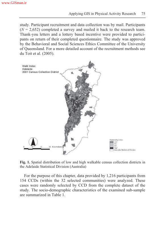
Applying GIS in Physical Activity Research 75

study. Participant recruitment and data collection was by mail. Participants

(N = 2,652) completed a survey and mailed it back to the research team.

Thank-you letters and a lottery based incentive were provided to partici-

pants on return of their completed questionnaire. The study was approved

by the Behavioral and Social Sciences Ethics Committee of the University

of Queensland. For a more detailed account of the recruitment methods see

du Toit et al. (2005).

Fig. 1. Spatial distribution of low and high walkable census collection districts in

the Adelaide Statistical Division (Australia)

For the purpose of this chapter, data provided by 1,216 participants from

154 CCDs (within the 32 selected communities) were analyzed. These

cases were randomly selected by CCD from the complete dataset of the

study. The socio-demographic characteristics of the examined sub-sample

are summarized in Table 1.

www.GISman.ir

76 Ester Cerin, Eva Leslie, Neville Owen and Adrian Bauman

Table 1. Socio-demographic characteristics of the sample (n = 1,216)

Characteristic Estimate Characteristic Estimate

Male, % 38.2 Education, %

Missing values 0.5 Year 10 or less 21.0

Employment status, % Year 12 / trade 28.5

Full time 39.5 Tertiary 46.8

Part time / casual / family 26.1 Missing values 3.7

Unemployed or home duties 13.6 Annual household

income, %

Retired / permanently un-

able to work

13.7 < $20,800 22.0

Other 5.1 $20,800 - $41,599 25.8

Missing values 1.9 $41,600 - $77,999 29.2

Age, mean (SD), y 42.8

(11.5)

> $77,999 18.2

Missing values, % 1.0 Missing values 4.8

Children in household, %

Yes 32.1

Missing values 1.0

2.2 Measures

2.2.1 Walkability Index (GIS-Based Community Walkability)

A Walkability Index was computed at the CCD level using GIS data on

four environmental attributes that have been found to be related to walking

(Saelens et al. 2003a). These were dwelling density, street connectivity,

net retail area and land-use mix (Frank and Pivo 1994). Dwelling density

was defined as the ratio of the number of dwelling units to the land area in

residential use (number of dwelling units per km2). Street connectivity was

defined as the ratio of the number of true intersections to the land area

(number of true intersections per km2). Figure 2 shows the map of a study

area with high residential density and street connectivity (suburb of Nor-

wood). A study area with low connectivity is shown in Figure 3.

Net retail area was represented by the average retail ratio of the retail

gross floor space to the land area. Finally, land-use mix represented the

degree to which different land uses were scattered within the land area.

Land-use mix was quantified as an entropy index. Land use was classified

into the following categories: residential, commercial, industrial, recrea-

tional and other. The entropy index was computed using the following

formula (Frank and Pivo 1994):

www.GISman.ir

Applying GIS in Physical Activity Research 77

N

ppk kk

ln

)ln( Eqn. (1)

where k is the category of land use; p is the proportion of the land area

within a CCD allocated to a specific land use; and N is the number of land

use categories (in our case, five). The entropy index ranges from 0 to 1,

with 0 representing homogeneity (all land uses are of a single type), and 1

representing maximal heterogeneity (the land use categories are evenly

represented in the CCD). The four environmental characteristics were

transformed into deciles and summed for each CCD, with a possible score

of 4 to 40, denoting the Walkability Index of a CCD (see Figure 1). Simi-

lar walkability indexes have been related to physical activity variables in

studies conducted in the Atlanta, Georgia (Frank et al. 2005) and Seattle,

Washington regions (Frank et al. 2006), supporting its validity and gener-

alizability.

Fig. 2. Map section representing a high density and high street connectivity study

area (suburb of Norwood, Adelaide, Australia); dots represent parcels in residen-

tial use

www.GISman.ir

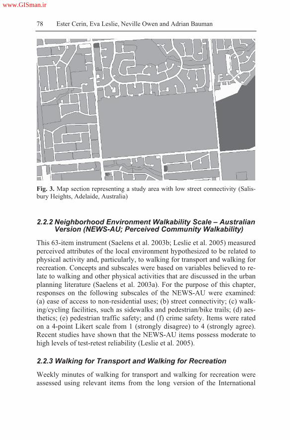
78 Ester Cerin, Eva Leslie, Neville Owen and Adrian Bauman

Fig. 3. Map section representing a study area with low street connectivity (Salis-

bury Heights, Adelaide, Australia)

2.2.2 Neighborhood Environment Walkability Scale – Australian Version (NEWS-AU; Perceived Community Walkability)

This 63-item instrument (Saelens et al. 2003b; Leslie et al. 2005) measured

perceived attributes of the local environment hypothesized to be related to

physical activity and, particularly, to walking for transport and walking for

recreation. Concepts and subscales were based on variables believed to re-

late to walking and other physical activities that are discussed in the urban

planning literature (Saelens et al. 2003a). For the purpose of this chapter,

responses on the following subscales of the NEWS-AU were examined:

(a) ease of access to non-residential uses; (b) street connectivity; (c) walk-

ing/cycling facilities, such as sidewalks and pedestrian/bike trails; (d) aes-

thetics; (e) pedestrian traffic safety; and (f) crime safety. Items were rated

on a 4-point Likert scale from 1 (strongly disagree) to 4 (strongly agree).

Recent studies have shown that the NEWS-AU items possess moderate to

high levels of test-retest reliability (Leslie et al. 2005).

2.2.3 Walking for Transport and Walking for Recreation

Weekly minutes of walking for transport and walking for recreation were

assessed using relevant items from the long version of the International

www.GISman.ir

Applying GIS in Physical Activity Research 79

Physical Activity Questionnaire (IPAQ; long last-7-days self-administered

format; Craig et al. 2003). A recent report on data collected in 12 countries

showed that the IPAQ had comparable reliability and validity to other self-

report measures of physical activity (Craig et al. 2003). The respondents

were instructed to report the frequency and duration of walking for trans-

port and walking for recreation during the past seven days. These items of

the IPAQ have been shown to possess good reliability (Vandelanotte et al.

2005) and adequate validity (Vandelanotte et al. 2005; Cerin et al. 2006).

In this study, total weekly minutes of walking for transport and for recrea-

tion were computed and values were truncated to 1860 minutes.

2.2.4 Socio-Demographic Attributes

Participants were asked to report their age, gender, educational attainment,

annual household income before taxes, employment status and number of

children under 18 years in the household.

2.3 Data Analyses

Multilevel confirmatory factor analysis (MCFA) was employed to define a

neighborhood-level measurement model for the NEWS-AU subscales with

items rated on a 4-point Likert scale. We used MCFA because this study

adopted a two-stage cluster sampling design and significant intraclass cor-

relations (ICCs), denoting the proportion of total item variance due to dif-

ferences between CCDs, were observed for all the NEWS-AU items

(Muthén 1997). MCFA was carried out using Bentler and Liang’s Maxi-

mum Likelihood Estimation (MLE) method (Bentler and Liang 2003).

This method uses an EM-type gradient algorithm for computing the MLE

for two-level structural equation models, of which confirmatory factor

analysis is a special case. This algorithm is applicable to any sample size

with balanced or unbalanced design and is preferable to other methods

when the sample sizes vary substantially among clusters (neighborhoods).

The end result of a MCFA is the estimation of a measurement model for

each level of variation (within- and between-neighborhoods). This chapter

focuses on between-neighborhood variations and, hence, a neighborhood-

level measurement model of the NEWS.

The construction of a two-level measurement model of the NEWS in-

cluded three main steps. The first two steps involved the assessment of two

a priori two-level measurement models. The first model encompassed six

oblique (correlated) factors, as originally defined by its developers (Sael-

ens et al. 2003b). For this model, the factor structures at the individual and

www.GISman.ir

80 Ester Cerin, Eva Leslie, Neville Owen and Adrian Bauman

neighborhood level were defined to be equal. The second a priori model

consisted of five correlated neighborhood-level factors, and six correlated

individual-level factors, emulating the empirically-based measurement

model of the original version of the NEWS (Cerin et al. 2006). In the third

step of the analyses, re-specification of the original model was conducted

according to Jöreskog and Sörbom’s (1993) iterative model-generating ap-

proach. This approach consists of testing the viability of initial hypotheti-

cal models in terms of whether they satisfactorily fit the observed data. If

the results indicate a lack of fit based on empirical or substantive evidence,

the models are re-specified. The ultimate goal of model re-specification is

to identify models that can provide a statistically acceptable fit and a theo-

retically meaningful interpretation of the data. Model re-specification was

based on the analysis of standardized factor loadings, the analysis of three

empirical indices of poor model fit (standardized residual covariances,

univariate Lagrange multiplier tests and Wald tests), and substantive con-

siderations (i.e., salience) (15). Factor loadings greater than |.30| were con-

sidered to be significant (Bryant and Yarnold 1994).

Several measures of absolute and incremental fit were used to evaluate

the goodness-of-fit of the measurement models. Absolute-fit indices de-

scribe the ability of the model to reproduce the original covariance matrix.

The absolute-fit indices reported in this chapter are the goodness-of-fit in-

dex (GFI) and the root mean square error of approximation (RMSEA). The

GFI describes the proportion of variance in the original data that is ac-

counted for by the proposed model, with values ranging from 0 (poor fit)

to 1.0 (perfect fit). The RMSEA estimates the average covariance residual

that would have been expected had the entire population of potential re-

spondents been represented, with values less than .08 indicating an accept-

able model fit. Two incremental fit indices, assessing the degree to which a

specified model is better than a baseline model that specifies no covari-

ances, were used. These were the non-normed fit index (NNFI) and the

comparative fit index (CFI). Values exceeding .90 are generally indicative

of an acceptable model fit. In addition to the above indices of fit, the stan-

dardized root mean squared residual (SRMR) was computed. The SRMR

is a standardized summary of the average covariance residuals. A favor-

able value for the SRMR is less than .10 (Browne and Cudeck 1993). All

MCFA analyses were performed using EQS 6.1 (Multivariate Software

Inc. 2004).

Multilevel linear models were used to estimate the magnitude of the

neighborhood-level associations between the GIS-based walkability in-

dex/components (neighborhood-level variables) and the MCFA-based

neighborhood-level NEWS-AU subscales. These models were also used to

estimate the neighborhood-level associations of the walkability index, its

www.GISman.ir

Applying GIS in Physical Activity Research 81

components and the NEWS-AU factors with weekly minutes of walking

for transport and walking for recreation. These associations were estimated

following the procedure specified by Snijder and Bosker (1993). A prob-

ability level of 0.05 was adopted. These analyses were performed using

MLwiN 2.02 (Multilevel Models Project, Institute of Education 2004).

3 Results

The two a priori models of the NEWS-AU did not adequately fit the ob-

served data. Hence, these models were re-specified following the proce-

dure described above. Table 2 reports the final between-neighborhood

measurement model (groups of items and underlying factors) of the

NEWS-AU. Three latent factors of perceived neighborhood environmental

attributes were found. All factor loadings were significant at a probability

level of .05 and their absolute values were greater than .42. These were

‘Access to services and ease of walking’, ‘Street connectivity’ and ‘Aes-

thetics, traffic and safety’. The first two factors were moderately positively

correlated (.48). All the goodness-of-fit indices indicated an acceptable fit

of the final measurement model to the data (GFI = .96; RMSEA = .052;

SRMR = .100; NNFI = .91; CFI = .90).

The descriptive statistics of, and correlations between, the walkability

index, its components and the NEWS-AU factors are shown in Table 3. A

reasonable degree of variability was observed in the objective and per-

ceived measures of neighborhood environmental attributes (see means and

standard deviations in Table 3). Ratings on the NEWS-AU factors of ‘Ac-

cess to services and ease of walking’ and ‘Street connectivity’ were mod-

erately to strongly correlated with the walkability index and its compo-

nents (r = 0.32 to 0.66), with the exception of land-use mix. No significant

associations were observed between the NEWS-AU factor ‘Aesthetics,

traffic and crime safety’ and the GIS-based measures of neighborhood

walkability.

www.GISman.ir

82 Ester Cerin, Eva Leslie, Neville Owen and Adrian Bauman

Table 2. Neighborhood-level measurement model of the NEWS-AU

Neighborhood-level

factor

Item content

- Can do most of the shopping

- Many shops within easy walking distance

- Many places to go within easy walking distance

- Easy to walk to a public transport stop

- Major barriers to walking [negatively scored]

- Footpaths on most of the streets

- Well-maintained footpaths

Access to services &

ease of walking

- Busy streets have pedestrian crossing / traffic signals

- Streets do not have many, or any, cul-de-sacs

- Walkways that connect cul-de-sacs to streets [nega-

tively scored]

- Short distance between intersections.

- Many four-way intersections

- Many alternative routes for getting from place to

place

Street connectivity

- Footpaths separated from the road/traffic by parked

cars

- Park or nature reserve in the local area

- Bicycle or walking paths in or near the local area

- Lots of greenery around the local area.

- Tree cover or canopy along the footpaths

- Many interesting things to look at while walking

- Local area free from litter, rubbish, or graffiti

- Many attractive buildings and homes

- Pleasant natural features

- A lot of traffic along the streets [negatively scored]

- Main arterial road or busy throughway for motor

vehicles nearby [negatively scored]

- A lot of exhaust fumes [negatively scored]

- A lot of petty crime [negatively scored]

- A lot of major crime [negatively scored]

- Level of crime makes it unsafe to walk during the day

[negatively scored]

- Level of crime makes it unsafe to walk at night

[negatively scored]

Aesthetics, traffic &

crime safety

- Feel safe walking home from a bus or train stop at

night

www.GISman.ir

Applying GIS in Physical Activity Research 83

Table 3. Neighborhood-level correlations between perceived and objective attrib-

utes of the neighborhood environment (154 CCDs)

GIS measures

WI DD ID NRA LUM

NEWS

factors

M (SD) 18.9

(5.5)

720.7

(304.3)

245.5

(156.4)

0.24

(0.20)

0.41

(0.19)

ASEW a 3.25 (0.64) 0.48* 0.32* 0.38* 0.48* 0.08

SCa

2.94 (0.63) 0.69* 0.48* 0.55* 0.65* 0.09

ATCSa

2.75 (0.74) -0.10 0.01 0.06 -0.10 0.02

M = mean; SD = standard deviation; ASWE = Access to service and ease of walk-

ing; SC = Street connectivity; ATCS = Aesthetics, traffic and crime safety; WI =

walkability index (possible range of values 4-40); DD = dwelling density (defined

as dwelling units per km2); ID = intersection density (defined as number of true in-

tersections per km2); NRA = net retail area (defined as the ratio of the gross retail

area to the total retail parcel area); LUM = land-use mix (possible range of values

0 – 1;); a possible range of values 1-4; * p <.05

Table 4. Neighborhood-level correlations of perceived and objective attributes of

the neighborhood environment with self-reported weekly minutes of walking for

transport

Objective measures R Perceived measures R

Walkability index .20* Access to services and ease of walking .27*

Dwelling density .45* Street connectivity .41*

Intersection density .27* Aesthetics, traffic and crime safety -.18

Net retail area .18

Land-use mix -.10

R = multiple correlation; * p < .05

Table 4 reports the univariate neighborhood-level associations of objec-

tive and perceived measures of neighborhood walkability with walking for

transport, adjusting for individual-level socio-economic factors. As no sig-

nificant neighborhood-level variation in walking for recreation was ob-

served, neighborhood-level associations between this type of walking and

objective/perceived attributes of the environment could not be computed.

The examined sample (N = 1,216) walked for transport on average 180

minutes a week (SD = 279 min/wk; Median = 85 min/week). Neighbor-

hood differences explained 1.4% of the variations in residents’ walking for

transport.

Significant positive associations were found between weekly minutes of

walking for transport and the GIS-based walkability index, dwelling den-

sity, and intersection density (Table 4). Although the relationship between

net retail area and walking for transport was in the expected direction, it

www.GISman.ir

84 Ester Cerin, Eva Leslie, Neville Owen and Adrian Bauman

was not statistically significant. Also, the data did not provide support for

an association between the GIS-based measure of land-use mix and walk-

ing for transport. As expected, two neighborhood-level factors of the

NEWS-AU hypothesized to be related to utilitarian walking were indeed

significantly related to weekly minutes of walking for transport. In con-

trast, the factor ‘Aesthetics, traffic and crime safety’ was not a reliable ex-

planatory variable of self-reported walking for transport. The multiple cor-

relation between the four GIS-based, objective measures of walkability

and walking was 0.47, whilst that between the three survey-based meas-

ures of perceived walkability and walking was 0.45.

4 Discussion

One of the main aims of this chapter was to examine the correspondence

between GIS-based, objective measures and survey-based, perceived

measures of neighborhood walkability in a sample of Australian adults.

Moderate to high levels of correspondence were found between perceived

neighborhood access to services, ease of walking, street connectivity and

all but one of the GIS-based measures of walkability. Specifically, no sig-

nificant association was observed between these perceived aspects of the

neighborhood environment and objective land-use mix. It is possible that

the lack of correspondence was due to the way land-use mix was opera-

tionalized. The measure of land-use mix used in this study was based on

the distribution of land area across different uses rather than, as recom-

mended, on the distribution of building floor space across different uses.

This can result in very different outcomes as, for example, a tall building

may contain over a million square feet of office and commercial use on a 1

acre (43,560 square foot site). However, adequate building square foot data

were not available for Adelaide (Australia). Also, while previous studies

used a measure of land-use mix which was exclusively based on categories

of land use that are thought to be conducive to walking for transport (e.g.,

commercial, residential, institutional, office; Frank et al. 2004; Frank et al.

2005), this study included an additional category of land use – namely,

recreational land use. Access to this type of land use is not captured by the

NEWS-AU factors of ‘Access to services and ease of walking’ and ‘Street

connectivity’. This could at least in part explain why no significant asso-

ciation was found between a GIS-based measure of objective land-use mix

and perceived attributes of the neighborhood environment thought to be re-

lated to utilitarian walking.

www.GISman.ir

Applying GIS in Physical Activity Research 85

The fact that the NEWS-AU factors ‘Access to services and ease of

walking’ and ‘Street connectivity’ were, but ‘Aesthetics, traffic and crime

safety’ was not related to the objective measures of walkability, gives sup-

port for the construct and criterion validity of the NEWS-AU as a measure

of neighborhood environmental attributes. As the GIS-based measures of

walkability were essentially measures of access to services and street con-

nectivity, it was logical to expect that these would show a significant asso-

ciation with their corresponding perceived neighborhood attributes

(NEWS-AU factors). Moreover, since the GIS-based measures of walk-

ability did not include information about aesthetic aspects of the neighbor-

hood environment, green areas, traffic load and safety from crime, it is not

surprising that no relationship was observed between the GIS-based walk-

ability measure and the respondents’ ratings on the factor ‘Aesthetics, traf-

fic and crime safety’.

The second main aim of this study was to examine the relationships of

objective and perceived attributes of the neighborhood environment with

walking for transport and walking for recreation. The associations between

the GIS-measures of walkability and walking for transport were, in the

main, significant and in the expected direction (i.e., positive). Contrary to

previous studies (Frank et al. 2004), no significant association was found

between objective land-use mix and walking for transport. As noted ear-

lier, this finding may be attributable to how land-use mix was operational-

ized. The index of land-use mix used in this study encompassed a compo-

nent (i.e., recreational land use) that is more likely to be associated with

walking for recreation. In this regards, Cerin et al. (in press) found that

residents of areas with access to commercial and industrial destinations re-

ported significantly more transport-related walking than did residents of

areas with access to recreational destinations, even if these areas had a

similar level of land-use mix. Indeed, recreational venues are likely to be

regularly visited less often and by fewer people (Sallis et al. 2004) and,

hence, their impact on residents’ transport-related walking is bound to be

limited.

Positive associations were also observed between some of the perceived

neighborhood attributes and walking for transport. As was the case for

their objective counterparts, perceived access to services and street con-

nectivity in the neighborhood of residence were predictive of higher levels

of walking for transport. Similar results have been recently reported in the

transport and urban planning literature and public health literature (Trans-

portation Research Board 2005). No significant associations were found

between walking for transport and perceived aesthetic features of the

neighborhood environment, traffic and safety from crime. This is some-

www.GISman.ir

86 Ester Cerin, Eva Leslie, Neville Owen and Adrian Bauman

what understandable as these are characteristics that haven been shown to

be more pertinent in relation to walking for recreation (Owen et al. 2004).

Importantly, in the present investigations, the GIS-based measure of

walkability was as good an explanatory variable of neighborhood differ-

ences in walking for transport as were residents’ perceptions of the

neighborhood environment. Both measures accounted for a significant

proportion of the neighborhood-level variance in walking for transport

(i.e., over 20%). This is an important finding supporting the utility of GIS

for the measurement of physical activity correlates and determinants. Ad-

ditionally, this particular finding suggest that the strength of association

between attributes of the built environment and walking behavior may be

substantially greater than previously noted. Studies examining the envi-

ronment-walking association at the individual level have reported only up

to 5% of shared variance between walking measures and specific aspects

of the environment (Transportation Research Board, 2005). These weaker

associations can be partly attributed to the fact that some individual differ-

ences in walking and perceived neighborhood environment are due to

measurement error (Cerin et al. 2006). An examination of the environ-

ment-walking association at the neighborhood level can partly eliminate

such problems. This is because the average rating given by a group of resi-

dents for the same neighborhood is likely to be a more reliable and valid

measure of the environment than is the rating of a single individual.

Finally, no significant association could be found between both objec-

tive and perceived neighborhood environmental attributes and walking for

recreation. This is because there was no neighborhood-level variation in

the respondents’ level of self-reported walking for recreation. This finding

can be easily explained by noting that, in this study, neighborhood selec-

tion was based on attributes that are relevant to walking for transport (e.g.,

street connectivity, dwelling density, and access to services) but irrelevant

to walking for recreation. Future research needs to focus on the develop-

ment of a GIS-based index of walkability suited to walking for recreation.

This index might include information on green areas, traffic load, presence

of footpaths, and proximity to beach or waterways, as suggested by recent

studies in the area of public health (Humpel et al. 2003).

5 Conclusions

In general, this study provides further support for the contention that as-

pects of the built environment are associated with specific forms of physi-

cal activity, and, hence, residents’ health. We have illustrated how GIS

www.GISman.ir

Applying GIS in Physical Activity Research 87

data were successfully used in the PLACE study to define and measure as-

pects of the built environment that are related to walking for transport. Im-

portantly, in the present investigation, a GIS-based measure of walkability,

grounded on the work of Frank and Pivo (1994), emerged to be as good an

explanatory variable of neighborhood differences in walking for transport

as residents’ perceptions of the neighborhood environment. This confirms

the utility of using GIS in physical activity research. This chapter has also

highlighted that there is still room for improvement in the operationaliza-

tion of GIS-based measures of neighborhood transport-related walkability.

There is also a need for the development of a walkability index appropriate

for walking for recreation.

Acknowledgements

The National Health and Medical Research Council (NHMRC) Project

Grant #213114 and NHMRC Program Grant #301200 supported the

PLACE (Physical Activity in Localities and Community Environments)

study. The authors are grateful to the South Australian Government de-

partment for Transport and Urban Planning for providing access to the

relevant GIS data used in this study. We thank Mr. Neil T. Coffee (Na-

tional Centre for the Teaching and Research into Social Application of

GIS, University of Adelaide) for computing the GIS-based walkability in-

dex and producing the maps presented in this chapter. We also thank Dr.

Poh-Chin Lai and the GIS laboratory of the Department of Geography,

University of Hong Kong for processing the images included in this chap-

ter.

References

[1] Bentler PM and Liang J (2003) Two-level mean and covariance structures:

maximum likelihood via an EM algorithm. In: Reise SP, Duan N (eds.) Multi-

level modeling: Methodological advances, issues, and applications. Lawrence

Erlbaum, Mahwah NJ, pp 53-70

[2] Browne MW and Cudeck R (1993) Alternative ways of assessing model fit.

In: Bolen KA, Long JS (eds.) Testing structural equation models. Sage Publi-

cations, Newbury Park CA, pp 136-162

[3] Bryant FB and Yarnold PR (1994) Principal-components analysis and ex-

ploratory and confirmatory factor analysis. In: Grimm LG, Yarnold PR (eds.)

Reading and understanding multivariate statistics. APA, Washington DC pp

99-136

[4] Cerin E, Leslie E, du Toit L, Owen N, Frank L (in press) Destinations that

matter: associations with walking for transport. Place Health

www.GISman.ir

88 Ester Cerin, Eva Leslie, Neville Owen and Adrian Bauman

[5] Cerin E, Saelens BE, Sallis JF, Frank LD (2006) Neighborhood Environment

Walkability Scale: validity and development of a short form. Med Sci Sports

Exerc 38:1682-1691

[6] Craig CL, Marshall AL, Sjöström M, Bauman A, Booth ML, Ainsworth BE,

Pratt M, Ekelund U, Yngve A, Sallis J, Oja P (2003) International Physical

Activity Questionnaire (IPAQ): 12-country reliability and validity. Med Sci

Sports Exerc 35:1381-1395

[7] du Toit L, Cerin E, Leslie E (2005) An account of spatially based survey

methods and recruitment outcomes of the Physical Activity in Localities and

Community Environments (PLACE) study. Cancer Prevention Research Cen-

tre, School of Population Health, The University of Queensland, Brisbane

Australia

[8] Frank L and Pivo G (1994) Impacts of mixed use and density on utilization of

three modes of travel: single-occupant vehicle, transit, and walking, Transport

Res Rec 1466:44-52

[9] Frank L, Andresen MA, Schmid TL (2004) Obesity relationships with com-

munity design, physical activity, and time spent in cars. Am J Prev Med

27:87-96

[10] Frank LD, Sallis JF, Conway T, Chapman J, Saelens B, Bachman W (2006)

Many pathways from land use to health: walkability associations with active

transportation, body mass index, and air quality. J Am Plann Assoc 72:75-87.

[11] Frank LD, Schmid TL, Sallis JF, Chapman J, Saelens BE (2005) Linking ob-

jectively measured physical activity with objectively measured urban form:

findings from SMARTRAQ. Am J Prev Med 28(2S2):117-125

[12] Hayashi T, Tsumura K, Suematsu C, Okada K, Fujii S, Endo G (1999) Walk-

ing to work and the risk for hypertension in men: The Osaka health survey.

Ann Intern Med 131:21-26

[13] Humpel N, Owen N, Leslie E, Marshall AL, Bauman AE, Sallis JF (2003)

Associations of location and perceived environmental attributes with walking

in neighborhoods. Am J Health Promot 18:239-242

[14] Jöreskog KG and Sörbom D (1993) Structural equation modeling with the

SIMPLIS command language. SPSS, Chicago IL

[15] King AC, Stokols D, Talen E, Brassington GS (2002) Theoretical approaches

to the promotion of physical activity. Am J Prev Med 23(S):15-25

[16] Leslie E, Coffee N, Frank L, Owen N, Bauman A, Hugo G (2007) Walkabil-

ity of local communities: Using Geographic Information Systems to objec-

tively assess relevant environmental attributes. Health Place 13:111-122

[17] Leslie E, Saelens B, Frank L, Owen N, Bauman A, Coffee N, Hugo G (2005)

Residents' perceptions of walkability attributes in objectively different

neighborhoods: a pilot study. Health Place 11:227-236

[18] Muthén BO (1997) Latent variable modeling of longitudinal and multilevel

data. In: Raftery AE (ed.) Sociological methodology (pp. 453-481) ASA,

Washington DC, pp 453-481

[19] Owen N, Humpel N, Leslie E, Bauman A, Sallis JF (2004) Understanding en-

vironmental influences on walking: review and research agenda. Am J Prev

Med 27:67-76

www.GISman.ir

Applying GIS in Physical Activity Research 89

[20] Rafferty AP, Reeves MJ, McGhee HB (2002) Physical activity patterns

among walkers and compliance with public health recommendations. Med Sci

Sports Exerc 34:1255-1261

[21] Saelens BE, Sallis JF, Frank LD (2003a) Environmental correlates of walking

and cycling: findings from the transportation, urban design and planning lit-

eratures. Ann Beh Med 25:80-91

[22] Saelens BE, Sallis JF, Black JB, Chen D (2003b) Neighborhood-based differ-

ences in physical activity: An environment scale evaluation. Am J Public

Health 93:1552-1558

[23] Sallis JF and Frank LD, Saelens BE, Kraft MK (2004) Active transportation

and physical activity: opportunities for collaboration on transportation and

public health research. Transport Res A 38:249-268

[24] Sallis JF and Owen N (2002) Ecological models of health behavior. In: Glanz

K, Lewis FM, Rimer BK (eds.) Health behavior and health education: theory,

research and practice. Jossey-Bass, San Francisco, pp 462-484

[25] Snijder TAB, Bosker B (1993) Modeled variance in two-level models. Sociol

Method Res 22: 342-363

[26] Transportation Research Board and Institute of Medicine (2005) Does the

built environment influence physical activity? Examining the evidence. Spe-

cial Report 282. National Academies Press, Washington DC

[27] United States Department of Health and Human Services (1996) Physical ac-

tivity and health: a report of the Surgeon General. Public Health Service, Cen-

ters for Disease Control and Prevention, National Centre for Chronic Disease

Prevention and Health Promotion, Atlanta GA

[27] Vandelanotte C, De Bourdeaudhuij I, Philippaerts R, Sjöström M, Sallis J

(2005) Reliability and validity of a computerized and Dutch version of the In-

ternational Physical Activity Questionnaire (IPAQ). J Phys Act Health 2:63-

75

www.GISman.ir

Objectively Assessing ‘Walkability’ of Local

Communities: Using GIS to Identify the Relevant

Environmental Attributes

Eva Lesliea, Ester Cerinb, Lorinne duToitc, Neville Owenc and Adrian

Baumand

a School of Health and Social Development, Deakin University, Australia b Institute of Human Performance, University of Hong Kong, HK, China c Cancer Prevention Research Centre, University of Queensland, Australia d NSW Centre for Physical Activity and Health, University of Sydney,

Australia

Abstract: Geographic Information Systems (GIS) may be used to

measure objectively, those features of the built environment that may

influence walking. Public health research on environmental determinants

of physical activity in adults shows that different factors can influence

walking for recreation, compared to walking for transport. Most studies

have used perceived (self-report) rather than objective measures of

potentially relevant environmental attributes. We describe how a

previously-developed index of ‘walkability’ was operationalized in an

Australian context, using available spatial data. Attributes believed to be of

relevance to walking for transport, that are measurable using GIS, are:

Dwelling density (higher-density neighborhoods support greater retail and

service variety, resulting in shorter, walkable distances between facilities;

driving and parking are more difficult and time consuming). Connectivity

(higher intersection densities provide people with a greater variety of

potential routes, easier access to major roads where public transport is

available and shorter times to get to destinations). Land use mix (the more

varied the land use mix and built form, then the more conducive it is to

walk to various destinations). Net retail area (there are more options for

destinations where goods and services may be purchased and more local

employment opportunities that can be reached by walking). The

associations of these attributes with walking behaviors can be examined

separately, or in combination. Such GIS data are very helpful in

fundamental studies of the environmental determinants of behavior, and

also in applied policy research for cities, regions or local communities, to

address public health and environmental issues.

www.GISman.ir

Assessing ‘Walkability’ of Local Communities Using GIS 91

Keywords: GIS, community walkability, walking for transport,

environment and public health.

1 Introduction

Physical inactivity is a major risk factor for overweight and obesity, diabe-

tes, heart disease and some cancers (USDHHS, 1996). In Australia, some

30 % of adults are sedentary in their leisure time (Owen & Bauman, 1997)

and over 50 % are insufficiently active to accrue health benefits (Booth et

al, 1997). Environmental and policy interventions form one of the major

strategic approaches to promoting participation in physical activity in in-

dustrialized countries (Sallis et al, 1998).

Researchers in both public health and the urban planning and transporta-

tion fields have highlighted the importance of using objective measures to

help better understand the relationships between physical environment at-

tributes and physical activity behaviors (Saelens et al, 2003; Sallis et al,

2004; Owen et al, 2004). Walking is the physical activity behavior that is

currently the main focus of environmental and policy initiatives in public

health (Owen et al, 2004). The ‘walkability’ of a community may be con-

ceptualized as the extent to which characteristics of the built environment

and land use may or may not be conducive to residents in the area walking

for either leisure, exercise or recreation, to access services, or to travel to

work. GIS provides methods that have the potential to facilitate the devel-

opment of indices of walkability at the local level in cities or regional ar-

eas, not only for the purposes of research, but also to evaluate new envi-

ronmental and policy initiatives (Sallis et al, 1998; Bauman et al, 2002).

Behavior-specific ecological models in population health identify a key

role for particular environmental attributes as determinants of specific

health-related behavioral choices (Bauman, Sallis & Owen, 2002; Sallis &

Owen, 2002). In the case of adults’ walking in local communities, the

choice to walk may be shaped by the cueing properties of environmental

attributes (for example, sidewalks, shade, accessible destinations); and, by

the reinforcing consequences of walking (for example, completion of er-

rands, use of recreational facilities) that are likely to increase the future

probability of choices to walk. Studies from the community design disci-

plines (particularly transportation and urban planning research) have iden-

tified some strong patterns of association (Frank et al, 2003). To date, there

are only a limited number of physical activity studies that have used envi-

ronmental variables derived objectively from GIS data (Frank et al, 2005;

Giles-Corti, 2002, 2003; Kirtland et al, 2003; Troped et al, 2001, 2003). A

www.GISman.ir

92 E. Leslie, et al.

feature of these studies is a specificity of focus (both on the environmental

attributes and the behavior) as there is an increasing body of evidence on

the correlates of specific behavioral physical activities and on the role of

particular environmental attributes (Humpel et al, 2002; Owen et al, 2004;

Trost et al, 2002). In the case of walking, different physical attributes of

local walking environments may be related to walking for particular pur-

poses, such as walking for exercise, pleasure or transport.

Building on research findings from the transportation, urban design and

planning fields, Saelens, Sallis and Frank (2003) argue that particular

physical elements of local environments influence residents’ choices to

walk. They describe aspects of local physical environments that are con-

sidered to influence walking for transport; two main dimensions of the way

land is used appear to be important: proximity (distance) and connectivity

(directions of travel). Proximity reflects two key land-use variables: den-

sity or compactness of land use; and, land use mix (the degree of heteroge-

neity with which functionally different uses are co-located in space). The

more compact and intermixed an urban environment is, the shorter the dis-

tances between destinations. Walking, relative to other modes of travel be-

comes less probable, as distances between origins and destinations in-

crease (Frank, 2004). Connectivity is the directness of routes between

households, stores, and workplaces. Walking is facilitated where there is a

lack of barriers (freeways and other physical obstacles) and where there

are a number of options for travel routes. Interconnecting streets laid out in

a regular grid pattern will act to facilitate walking for transport (Saelens,

Sallis & Frank, 2003; Frank, Engelke & Schmid, 2003).

The aim of this chapter is to describe the construction of an objective,

GIS-based measure of community walkability (walkability index) based on

key environmental characteristics related to walking for transport. This in-

dex of walkability is designed to reflect utilitarian forms of walking to

work, shops and other daily destinations rather than walking for recreation

and leisure. The applications, limitations and potential for further devel-

opment of the walkability index are discussed.

2 Methods

2.1 Using Australian GIS data to derive a walkability index

The potential walkability dimensions of proximity and connectivity de-

scribed above can be readily operationalized using GIS methods. A num-

ber of approaches have previously been used to measure walkability and

the connectivity of different neighborhood designs (Aultman-Hall et al,

www.GISman.ir

Assessing ‘Walkability’ of Local Communities Using GIS 93

1997; Cervero & Kockelman, 1997; Handy, 1996; Hess, 1997; Greenwald

& Boernet, 2001; Randall & Baetz, 2001). The spatial index of walkability

described in this chapter is built upon the method originally developed by

Frank and colleagues in the USA (Frank et al, under review) for use in the

Neighborhood Quality of Life Study (NQLS; see www.nqls.org). The

USA and Australian research teams collaborated on the adaptation of the

walkability index for use with readily available Australian GIS databases.

The index was subsequently used to generate a sampling frame for the

PLACE (Physical Activity in Localities and Community Environments)

study, conducted in Adelaide, the capital city of South Australia (Leslie et

al, in press).

2.2. Measures

Spatial data sets used included tax valuation and cadastral (parcel) data,

street centerline data, land use, zoning data, shopping centre location data

integrated within a GIS to create an environmental characteristic index at

the Census Collection District (CCD) level. In Australia, a CCD is the

smallest unit for which population census data is made available. The fol-

lowing sections describe how each attribute was measured. The implied re-

lationship to walking for transport for each of the measures calculated for

the walkability index are summarized in Table 1.

Table 1. Elements of environmental characteristics and relationships to walking

behavior (From Leslie et al, in press)

Environmental

attribute

Implied Relationship with Walkability GIS Databases

to Identify the

Attribute

Dwelling

density

High-density neighborhoods include

mixed-use development - improves ac-

cessibility to variety of complementary

activities and thus, increased utility

Associated with increases in retail and

service variety, resulting in shorter,

walkable distances between complemen-

tary shops and restaurants

Driving and parking more difficult and

time consuming

Dwellings data

Connectivity Higher intersection densities are corre-

lated with increased network connec-

tivity, thus providing people with a

greater variety of potential routes

Higher connectivity provides easier ac-

Road centre line

and intersec-

tions data

www.GISman.ir

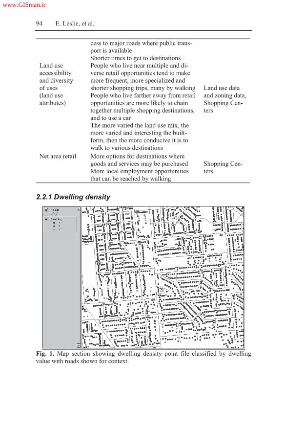
94 E. Leslie, et al.

cess to major roads where public trans-

port is available

Shorter times to get to destinations

Land use

accessibility

and diversity

of uses

(land use

attributes)

People who live near multiple and di-

verse retail opportunities tend to make

more frequent, more specialized and

shorter shopping trips, many by walking

People who live farther away from retail

opportunities are more likely to chain

together multiple shopping destinations,

and to use a car

The more varied the land use mix, the

more varied and interesting the built-

form, then the more conducive it is to

walk to various destinations

Land use data

and zoning data,

Shopping Cen-

ters

Net area retail More options for destinations where

goods and services may be purchased

More local employment opportunities

that can be reached by walking

Shopping Cen-

ters

2.2.1 Dwelling density

Fig. 1. Map section showing dwelling density point file classified by dwelling

value with roads shown for context.

www.GISman.ir

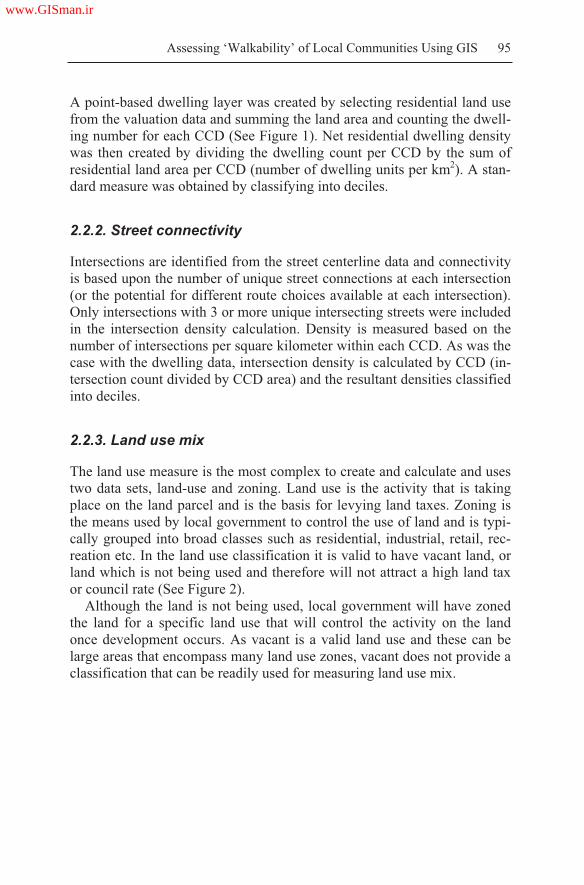
Assessing ‘Walkability’ of Local Communities Using GIS 95

A point-based dwelling layer was created by selecting residential land use

from the valuation data and summing the land area and counting the dwell-

ing number for each CCD (See Figure 1). Net residential dwelling density

was then created by dividing the dwelling count per CCD by the sum of

residential land area per CCD (number of dwelling units per km2). A stan-

dard measure was obtained by classifying into deciles.

2.2.2. Street connectivity

Intersections are identified from the street centerline data and connectivity

is based upon the number of unique street connections at each intersection

(or the potential for different route choices available at each intersection).

Only intersections with 3 or more unique intersecting streets were included

in the intersection density calculation. Density is measured based on the

number of intersections per square kilometer within each CCD. As was the

case with the dwelling data, intersection density is calculated by CCD (in-

tersection count divided by CCD area) and the resultant densities classified

into deciles.

2.2.3. Land use mix

The land use measure is the most complex to create and calculate and uses

two data sets, land-use and zoning. Land use is the activity that is taking

place on the land parcel and is the basis for levying land taxes. Zoning is

the means used by local government to control the use of land and is typi-

cally grouped into broad classes such as residential, industrial, retail, rec-

reation etc. In the land use classification it is valid to have vacant land, or

land which is not being used and therefore will not attract a high land tax

or council rate (See Figure 2).

Although the land is not being used, local government will have zoned

the land for a specific land use that will control the activity on the land

once development occurs. As vacant is a valid land use and these can be

large areas that encompass many land use zones, vacant does not provide a

classification that can be readily used for measuring land use mix.

www.GISman.ir

96 E. Leslie, et al.

Fig. 2. Map section showing the Planning South Australia land use groupings.

(Notice the large area in the top left is classified as vacant under land use).

To overcome the problem of large vacant areas and the potential to skew

the land use mix calculation, the underlying local government zoning is

used to reclassify vacant parcels to the local government zoning (See Fig-

ure 3). In this way, the intended land use (zoning) is used in place of the

vacant land use for the purpose of calculating the land use mix measure.

Once the vacant land is replaced with a land use zone, the land uses are re-

classified into the following five classes, residential, commercial, indus-

trial, recreation and other.

The sum of land area by CCD is used to create an entropy score for each

CCD, calculated via the following formula, where k is the category of land

use; p is the proportion of the land area devoted to a specific land use; N is

the number of land use categories:

N

ppk kk

ln

ln

www.GISman.ir

Assessing ‘Walkability’ of Local Communities Using GIS 97

Fig. 3. Map section showing the Planning South Australia zoning (intended land

use) groupings. Note the large vacant area (top left) from Fig.2 is designated as ru-

ral living under zoning.

The entropy equation results in a score of 0 to 1, with 0 representing

homogeneity (all land uses are of a single type), and 1 representing hetero-

geneity (the developed area is evenly distributed among all land use cate-

gories). The entropy land use score for each CCD is joined to the CCD

theme and classified into deciles with the 1st decile recoded to 1 represent-

ing CCDs with the least land use mix and the 10th decile recoded to 10 rep-

resenting CCDs with the most mixed land uses.

2.2.4. Net area retail

The final measure in the walkability index is net retail area. A Retail Data

Base is a collection of all retail activity in shopping centers with three or

more shops or a single shop 250 square meters or larger. Field survey

teams visit all centers and measure the gross retail area, the parcel area, re-

tail activity and a range of other data. It is the gross retail area and the par-

cel area that are used in this measure as a simple ratio: NRA = GRA / P;

(where GRA = gross retail area; and, P = total retail parcel area).

The premise for this measure is to calculate the amount of retail floor

area in relation to the total amount of land area that serves retail use. As a

result, this measure captures the degree to which retail is located near the

roadway edge, as is the case in a pedestrian oriented community, or set be-

hind a sea of parking. A ratio of 1 (retail space=total parcel space) or

greater than 1 indicates retail areas where less space is devoted to cars and

www.GISman.ir

98 E. Leslie, et al.

where distances between building entrances, transit, and other activities as

shortened. Most importantly, pedestrians in locations with a high retail

floor area ratio are less likely to be confronted with dangerous auto domi-

nated environments such as large parking lots that sever sidewalks from

building entrances. The net retail area ratio is calculated for each CCD and

classified into deciles.

2.3. The walkability index

The four environmental characteristics were all transformed into deciles

and summed for each CCD, with a possible score of 4 to 40, to denote the

walkability index. This score was then classified into quartiles with the 1st

quartile used to identify low walkability CCDs and the 4th quartile identify-

ing high walkability CCDs. These indexes can then be mapped to visually

identify areas at the extremes of walkability.

3 Results

Field validation was conducted to check the performance of the walkabil-

ity index and determine how well the method worked as a means of sorting

areas on the basis of environmental attributes which support walking be-

havior. The majority of selected areas’ physical characteristics accorded

with the classification of walkability objectively derived in GIS. Through

an extensive field observation process, the study team determined that the

methodology does return a face-valid means of identifying areas based

upon the input characteristics of dwelling data, land use and zoning, inter-

section data and net retail area.

In addition, an earlier study comparing residents’ perceptions of walk-

ability attributes in objectively different neighborhoods at the extremes of

walkability, found that residents of high and low-walkable neighborhoods

could reliably perceive the objective differences between them (Leslie et

al, 2005). This earlier study used only three components for measuring

walkability (net retail area was not included). Figure 4 shows the mean

subscale scores for residents in high and low walkable neighborhoods.

Comparison of scores shows that residents in the high-walkable neighbor-

hoods provided ratings indicative of higher residential density, land use

mix-diversity, land use mix access, street connectivity and infrastructure

for walking (all p<.001) than did residents of low-walkable neighborhoods.

www.GISman.ir

Assessing ‘Walkability’ of Local Communities Using GIS 99

Fig. 4. Comparison of mean scores for perceived environmental characteristics for

residents in high- and low-walkable neighborhoods (all statistically significantly

different, p<.001). Adapted from Leslie et al, 2005.

4 Discussion

The four environmental characteristics utilized in the method described

above are a starting point to a more detailed and informed measure of

walkability. There are plausibly many other factors linked with walking

behavior that warrant further consideration. However, it should be noted

that while there may be a range of factors that are worthy of consideration,

data is specific to particular areas and it may not be possible to include a

large range of the same factors across different areas.

Applications

The walkability index and its component measures, provides a useful tool

for the selection of communities for household recruitment, as it can

maximize the variability in the built environment and result in an improved

ability to detect differences in physical activity levels that likely occur in

objectively different environments. Selecting communities based on ex-

tremes of walkability is currently being promoted by the International

Physical Activity and the Environment Network (www.ipenproject.org) to

0

0.5

1

1.5

2

2.5

3

3.5

4

Density Land use

diversity

Land use

access

Connectivity Aesthetics

HIGH walkable LOW walkable

www.GISman.ir

Assessing ‘Walkability’ of Local Communities Using GIS 101

could examine a wider range of GIS variables for their relation to physical

activity, with the eventual aim of creating a more comprehensive walkabil-

ity index.

As with any use of GIS data there are also issues of data quality and in-

tegrity. For example, boundaries and attributes may no longer match if the

data has been collected at various timepoints. Some data may be incom-

plete or may include variation as a result of being constructed at various

stages and accuracy for some attributes could be ambiguous or may lack

sufficient detail. There will naturally be a need to make assumptions and

decisions along the way in working with any ‘raw’ data and this will vary

according to who is working with it.

Further development of the walkability index

A further development in the application of the walkability index in public

health, transport and planning research is to use these characteristics at the

individual residence level. Many of the elements involved in the derivation

of the index of walkability are applicable at an individual residence level

and it would be desirable to calculate the index for each individual resi-

dence. This would require identifying the relevant boundaries around each

residential location, within which the measures of relevant attributes can

be derived and an individual walkability score calculated. This would al-

low a surface of walkability to be derived which could then be aggregated

to any desired spatial level to protect confidentiality and for further analy-

sis. For example, new measures that allow for assessment of walking

within (10-15 minute walk from home) and outside local neighborhoods

have recently been developed (Giles-Corti et al, 2006). These can be used

against GIS methods that increase the specificity of a neighborhood walk-

ability measure by using smaller spatial units based on a resident’s loca-

tion. Methods for increasing such specificity are currently being developed

(Learnihan et al, 2006). It is anticipated that refined measures that include

additional elements and that build upon the actual residential location may

provide a more robust measure with a greater range of inputs, be spatially

more flexible and can be aggregated to a multitude of geographic scales at

the observation, community, sub-area, and regional scale.

www.GISman.ir

102 E. Leslie, et al.

5 Conclusion

There are a wide array of potential applications of GIS methods for guid-

ing environmental and policy initiatives to promote walking and to in-

crease overall physical activity levels. Increased computing capabilities, in

concert with the availability of GIS based land use and transportation data

provide considerable opportunity to develop objective measures of the

built environment that form independent predictors of human activity pat-

terns.

Acknowledgements

We thank Neil Coffee and the National Centre for Social Applications of

GIS (GISCA) at the University of Adelaide for technical support. The Na-

tional Health and Medical Research Council (NHMRC) Program Grant

#301200 supported the PLACE (Physical Activity in Localities and Com-

munity Environments) study. Dr Leslie is supported by an NHMRC Public

Health Fellowship # 301261.

References

[1] Aultman-Hall L, Roorda M, Baetz BW (1997) Using GIS for evaluation of

neighborhood pedestrian accessibility. Journal of Urban Planning and Devel-

opment 123(1):10-17

[2] Bauman A, Sallis JF, Owen N (2002) Environmental and policy measurement

in physical activity research. In Welk G & Dale D (Eds.), Physical activity

assessments for health-related research. Champaign, Illinois: Human Kinet-

ics, pp. 241-251

[3] Booth ML, Bauman A, Owen N, Gore CJ (1997) Physical activity prefer-

ences, preferred sources of assistance and perceived barriers to increased ac-

tivity among physically inactive Australians. Preventive Medicine, 26:131-7

[4] Cervero R and Kockelman K (1997) Travel demand and the 3Ds: Density, di-

versity, and design. Transportation Research Part D, 2(3):199-219

[5] Frank LD (2004) Economic determinants of urban form. Resulting trade-offs

between active and sedentary forms of travel. American Journal of Preventive

Medicine 27(3S): 146-153

www.GISman.ir

Assessing ‘Walkability’ of Local Communities Using GIS 103

[6] Frank L, Andresen MA, Schmid TL (2004) Obesity relationships with com-

munity design, physical activity, and time spent in cars. American Journal of

Preventive Medicine 27(2):87-96

[7] Frank LD, Engelke PO, Schmid TL (2003) Health and community design.

The impact of the built environment on physical activity. Washington: Island

Press

[8] Frank LD, Sallis JF, Saelens BE, Leary LE, Cain K, Conway T (manuscript

under review). Assessing the relation between urban form and physical activ-

ity: design and methods of the Neighborhood Quality of Life Study

[8] Frank LD, Schmid TL, Sallis JF, Chapman J, Saelens BE (2005) Linking ob-

jectively measured physical activity with objectively measured urban form.

American Journal of Preventive Medicine 28(2S2):117-125

[9] Giles-Corti B and Donovan RJ (2002) The relative influence of individual,

social and physical determinants of physical activity. Social Science and

Medicine 54(12):1793-1812

[10] Giles-Corti B and Donovan RJ (2003) Relative influences of individual, so-

cial environmental and physical environmental correlates of walking. Ameri-

can Journal of Public Health 93(3):1583-1589

[11] Giles-Corti B, Timperio A, Cutt H, Pikora TJ, Bull FCL, Knuiman M, et al.

(2006) Development of a reliable measure of walking within and outside the

local neighborhood: RESIDE's Neighborhood Physical Activity Question-

naire. Preventive Medicine 42:455-459

[12] Greenwald MJ and Boarnet MG (2001) The built environment as a determi-

nant of walking behavior: Analyzing non-work pedestrian travel in Portland,

Oregon. Transportation Research Record 1780:33-43

[13] Handy SL, Boarnet MG, Ewing R, Killingsworth RE (2002) How the built

environment affects physical activity. Views from urban planning. American

Journal of Preventive Medicine 23(2S):64-73

[14] Hess PM (1997) Measures of connectivity. Places 11:58-65

[15] Humpel N, Owen N, Leslie E (2002) Environmental factors associated with

adults’ participation in physical activity: A review. American Journal of Pre-

ventive Medicine 22(3):188-99

[16] Kitamura R, Mokhtarain PL, Laidet L (1997) A micro-analysis of land use

and travel in five neighborhoods in the San Francisco Bay area. Transporta-

tion 24:125-128

[17] Kirtland KA, Porter DE, Addy CL, Neet MJ, Williams JE, Sharpe PA, et al.

(2003) Environmental measures of physical activity supports: Perception

versus reality. American Journal of Preventive Medicine 24(4):323-331

[18] Learnihan V, Van Niel K, Giles-Corti B (2006) Walking and the built envi-

ronment. The influence of data scale in walkability analyses: results from

RESIDE. Abstract in Fifth Conference of the International Society for Behav-

ioral Nutrition and Physical Activity, ISBNPA, Boston, USA, p.240

[19] Leslie E, Saelens B, Frank L, Owen N, Bauman A, Coffee N, et al. (2005).

Residents' perceptions of walkability attributes in objectively different

neighborhoods: a pilot study. Health and Place 11:227-236

www.GISman.ir

104 E. Leslie, et al.

[20] Leslie E, Coffee N, Frank L, Owen N, Bauman A, Hugo G (in press, available

on line). Walkability of local communities: using Geographical Information

Systems to objectively assess relevant environmental attributes. Health and

Place

[21] Owen N and Bauman A (1997) The descriptive epidemiology of a sedentary

lifestyle in adult Australians. International Journal of Epidemiology

21(2):305-10

[22] Owen N, Humpel N, Leslie E, Bauman A, Sallis JF. (2004) Understanding

environmental influences on walking: review and research agenda. American

Journal of Preventive Medicine 27(1):67-76

[23] Pikora TJ, Bull FCL, Jamrozik K, Knuiman M, Giles-Corti B, Donovan RJ

(2002) Developing a reliable audit instrument to measure the physical envi-

ronment for physical activity. American Journal of Preventive Medicine

23(3):187-194

[24] Randall TA and Baetz BW (2001) Evaluating pedestrian connectivity for

suburban sustainability. Journal of Urban Planning and Development 127:1-

15

[25] Rodriguez DA and Joo J (2004) The relationship between non-motorized

mode choice and the local physical environment. Transportation Research

Part D, 9:151-173

[26] Sallis J, Bauman A, Pratt M (1998) Environmental and policy interventions to

promote physical activity. American Journal of Preventive Medicine 15(4):

379-97

[27] Saelens BE, Sallis JF, Frank LD (2003) Environmental correlates of walking

and cycling: Findings from the transportation, urban design, and planning lit-

eratures. Annals of Behavioral Medicine 25(2):80-91

[28] Sallis JF, Frank LD, Saelens BE, Kraft MK (2004) Active transportation and

physical activity: opportunities for collaboration on transportation and public

health. Transportation Research Part A, 38:249-268

[29] Sallis JF and Owen N (2002) Ecological models of health behavior. In: Glanz

K, Lewis FM, Rimer BK. (eds.) Health Behavior and Health Education: The-

ory, Research, and Practice. 3nd ed. San Francisco: Jossey-Bass, pp. 462-484

[30] Trost SG, Owen N, Bauman AE, Sallis JF, Brown W (2002) Correlates of

adults participation in physical activity: review and update. Medicine and Sci-

ence in Sports and Exercise 34(12):1996-2001

[31] Troped PJ, Saunders RP, Pate RR, Reininger B, Addy CL (2003) Correlates

of recreational and transportation physical activity among adults in a New

England community. Preventive Medicine 37:304-310

[32] United States Department of Health and Human Services (1996) Physical Ac-

tivity and Health: A Report of the Surgeon General. Atlanta, GA: Public

Health Service, Centers for Disease Control and Prevention, National Centre

for Chronic Disease Prevention and Health Promotion

www.GISman.ir

Developing Habitat-suitability Maps of Invasive

Ragweed (Ambrosia artemisiifolia.L) in China

Using GIS and Statistical Methods

Hao Chena,b, Lijun Chenb, and Thomas P. Albrightc

a School of Remote Sensing Information Engineering, Wuhan university,

Wuhan, China, b National Geomatics Centre of China, Beijing, China, c Department of Zoology, University of Wisconsin-Madison, WI, USA

Abstract: Invasive alien species pose a large and growing threat to the

economy, public health, and ecological integrity in China. Ragweed (Am-

brosia artemisiifolia.L), native to North America, was first documented in

China in 1935. As the primary pathogen of pollinosis, ragweed has become

a serious menace to public health of China’s population. Explaining and

predicting the spatial distribution of ragweed is of great importance to pre-

vention and early warning efforts. We studied the potential distribution of

ragweed, the environmental factors that influence its distributions, as well

as the ability to compute habitat-suitability maps using GIS and statistical

tools. We have developed models using logistic regression based on her-

barium specimen locations and a suite of GIS layers including climatic, to-

pographic, and land cover information. Our logistic regression model was

based on Akaike’s Information Criterion (AIC) from a suite of ecologi-

cally reasonable predictor variables. Based on the results, we provided a

new method to compartmentalize the habitat-suitability in the native range.

Finally, we used the model and the compartmentalized criterion developed

in the native range to “project” a potential distribution onto the exotic

ranges to build habitat-suitability maps.

Keywords: invasive species, habitat-suitability maps, Akaike’s Informa-

tion Criterion (AIC), logistic regression, quantile, GIS

1 Introduction

Invasive alien species pose a growing threat to the economy, public health,

and ecological integrity of nations worldwide. The invasions on local eco-

www.GISman.ir

Developing Habitat-suitability Maps of Invasive Ragweed in China 107

consists only of presence data sets. In order to decrease this sampling bias,

we proposed a new approach specifically to compartmentalize the habitat-

suitability using logit value threshold and the quantile statistics.

2 Methods

2.1 Study Species

Ragweed, originally found in North America, is an annual herbaceous

plant. It is a well-documented cause of seasonal allergic rhinitis and sea-

sonal asthma for countries in the Northern Hemisphere such as the United

States and Canada (Creticos et al. 1996, Boulet et al. 1997). It appeared

that Ragweed accidentally intruded china and was discovered in northeast

China for the first time in 1935. It then rapidly spread to northern and cen-

tral China, covering 15 provinces, but its ability to continue its invasion

into other regions of China is unknown. By 2004 and in Jilin province

alone, there were over 150,000 people suffering from the pollinosis related

to ragweed with more than 530,000 hectares of farmland threatened by re-

source competition from ragweed (Cui et al. 2004). The aim of this chapter

was to predict the potential future distribution of this species based on its

habitat suitability.

2.2 Species Data

Habitat-suitability models were based on 243 unique georeferenced her-

barium specimen records derived from the native range (USA and Canada)

of ragweed accumulated from museum collections and databases (see Ac-

knowledgments) An additional 83 points from the species’ invaded range

(China) were gathered from the herbarium museum of the Kunming Insti-

tute of Botany and the herbarium museum of the Institute of Botany of the

Chinese Academy of Sciences. The occurrences of ragweed are shown in

Figure 1. Because we have no absence data for ragweed, we generated

“pseudo-absence” data by selecting points at random from the geographi-

cal space in the native range. All occurrence points were georeferenced to

a precision finer than the 0.167 degree of latitude and longitude grain size

used for the modeling.

www.GISman.ir

108 Hao Chen, Lijun Chen and Thomas P. Albright

Fig. 1. Distribution of herbarium specimen records for ragweed ( ) in native

(North America) and invaded ranges (China)

2.3 Selection of Habitat Variables

Many potential predictors were either different measures of the same eco-

logical characteristic or were calculated using the same data, thus inherit-

ing problems of collinearity (Legendre and Legendre 1998). For this rea-

son, six biologically relevant environmental factors were considered for

inclusion in the analysis (Table 1). They included elevation (Elev), mean

annual precipitation (Precip), minimum temperature of the coldest month

(Mintmp), percent of maximum solar radiation (Sun), the proportion of ar-

eas devoted to either agricultural or urban land uses (Agurb), and percent

forest cover (Fordens). Although these data were collected from sources of

variable scales, they were all converted to the same resolution level of

0.167° 0.167° (about 15 15 km2 for the middle latitudes of China).

Altitude was selected as a variable because of its influence in the cli-

matic conditions of the ragweed that result in changes to the vegetation

and the timing and length of fruit bearing and flowering seasons. Precipita-

tion has the potential impact on soil moisture and the water balance of

ragweed. Minimum temperature and solar radiation are both essential fac-

tors to the growth of ragweed. The interaction terms including (Sunshine *

Minimum temperature) and (Precipitation * Minimum temperature) may

be important for the plant in periods of short daylight. The four coverages

were all from CRU CL 2.0 (New et al. 2002) and Worldclim 1.4

(http://biogeo.berkeley edu/worldclim/worldclim.htm). Human disturbance

is very important for the expansion and persistence of many invasive

plants, including ragweed, and the percentage of agriculture and urban

landuse (derived from the USGS Global Landcover Characterization data-

set) (Loveland et al. 2000) was thought to be a reasonable proxy for this.

Finally, density of forest cover came from the UN/FAO Forest Resources

Assessment 2000 dataset (Waller and Zhu 1999).

www.GISman.ir

Developing Habitat-suitability Maps of Invasive Ragweed in China 109

Table 1. Prior knowledge of predictor variables and their abbreviations used in the

model

Abbreviation Predictor Vari-

ables

Description

Elev Elevation Elevation may influence associated cli-

matic conditions.

Precip Precipitation Precipitation has the potential to influ-

ence soil moisture and the water balance

of ragweed.

Mintmp Min temperature

of coldest month

Ragweed is very sensitive to low tem-

peratures.

Sun Sunshine Percent of maximum possible solar radia-

tion is very important for the plant under

short days.

Agurb Density of agricul-

ture and urban

Human settlement may influence the

spread of ragweed.

Fordens Density of forest Treeless areas may not support popula-

tion. On the other hand, very high forest

cover may limit opportunities.

2.3 Statistical Analyses

Binary Logistic Regression

We used the GLM to predict the potential distribution of ragweed based on

presence points and “pseudo-absence” data in their native range. As the re-

sponse variable of this analysis was binary, the appropriate form of GLM

was binomial logistic regression (Guisan and Zimmermann 2000). The

probability of the species occurrence is calculated as follows:

0 1 1 2 2

0 1 1 2 2

...

...( ) ,

1

K K

K K

B B X B X B X

B B X B X B X

eprobability even

e

Eqn. 2.1

where B0 to Bk are coefficients, X1 to Xk are the independent variables. Lo-

gistic regression analysis was in the R statistical package. Initially three

variables (Precip, Mintmp, and Sun) and their second order terms were in-

cluded in a core model. We used a stepwise approach to add the other vari-

ables to the basic model to build more complicated models using logistic

regression. The additional variables included Elev, Agurb, Fordens and

their second order terms and two interaction terms: Sun* Mintmp and Pre-

cip * Mintmp.

www.GISman.ir

110 Hao Chen, Lijun Chen and Thomas P. Albright

Akaike’s Information Criterion (AIC)

The selection of the logistic regression model was based on Akaike’s In-

formation Criterion (AIC). AIC represents the relationship between the

maximum likelihood and Kullback-Leibler information. It is based on the

principle of parsimony (by including a penalty for the number of parame-

ters) and attempts to select a good approximating model (Anderson et al.

2000, Burnham and Anderson 2002). AIC is defined as:

eˆL | data 2K,AIC 2 log Eqn. 2.2

where eˆL | data2 log is the value of the maximized-log-likelihood

over the unknown parameters (ˆ), given the data and the model, and K is

the number of estimable parameters included in the model (number of

variables + the intercept).

The models can then be ranked from best to worst using the delta AIC

( i), which is a measure of each model relative to the best model, and is

calculated as:

i iDelta AIC AIC min AIC, Eqn.2.3

where AICi is the AIC value for model i , and minAIC the AIC value of

the best model. We ran each of the models and computed the AIC and i

in the R statistical package. Akaike weights ( wi ) provide another measure

of the strength of evidence for each model, and represent the probabilities

that model i is the Kullback–Leibler best model in the whole set of R can-

didate models:

i

exp / 2w .

exp / 2

I

R

I

r i

Eqn. 2.4

A weighted average was calculated for the coefficient of each parameter

for the average model using the equation below, i is the coefficient

for model i.

1

model-averaged estimate .R

i i

i

wEqn. 2.5

www.GISman.ir

Developing Habitat-suitability Maps of Invasive Ragweed in China 111

The assessment of relative importance of the predictor variables can be

made by summing the Akaike weights for all models containing a given

predictor variable rather than a single selected model (Burnham and

Anderson 2001).

2.4 Habitat-suitability Compartmentalization

Calculation of the Logit Value

Having obtained the weighted average model and their regression coeffi-

cients (see Table 3), the resulting regression equations were applied to the

native samples including the presence points and “pseudo-absence” points

to produce the output of the logit value. The final function takes the form

of:

2 2log precip precip mintmp mintmp sun0 1 2 3 4 5

2 2 2 sun elev elev fordens fordens agurb6 7 8 9 10 11

2 agurb (sun * mintmp) *(precip * mintmp)12 13 14

it Eqn.2.6

Re-class for the Samples

Because of the lack of true absence data, it was not be possible to calculate

meaningful probabilities from the logit values. Instead, we developed a

method, inspired by resource selection functions (Manly et al. 2002), to

map relative suitability values based on logit thresholds and quantiles.

Firstly, we defined a suitability threshold based on the minimum logit

value of reference presence points in the native range. As an alternative,

we also determined this threshold from the invaded range data. The

threshold allowed us to place every pixel broadly into either suitable or un-

suitable categories depending on whether its modeled logit value exceeded

or was less than the threshold. Finally, we calculated quartiles for each of

these two groups using the quantile function (Hyndman and Fan 1996) in

the R statistical package. The resulting eight classes ranked from the most

unsuitable to the most suitable are as below:

www.GISman.ir

112 Hao Chen, Lijun Chen and Thomas P. Albright

Unsuitable < minimum logit

1 most unsuitable < first quartile of unsuitable samples

2 first quartile of unsuitable samples ~ second

quartile of unsuitable samples.

3 second quartile of unsuitable samples ~ third

quartile of unsuitable samples

4 slightly unsuitable third quartile of unsuitable samples ~ minimum

logit

Suitable > minimum logit

5 slightly suitable minimum logit ~ first quartile of suitable samples

6 first quartile of suitable samples ~ second quartile

of suitable samples

7 second quartile of suitable samples ~ third

quartile of suitable samples

8 most suitable > third quartile of suitable samples

Compute the Habitat-suitability Map

Logit values were then calculated for every pixel in ERDAS 8.6 for both

native (North America) and invaded (China) ranges, according to the

Equation 2.6 and Table 3. The resulting maps of logit values were then

categorized into the eight suitability classes.

Because of the geographic and floristic similarities between China and

North America, we used the habitat-suitability models developed from na-

tive ranges to “project” onto the exotic ranges to predict the ragweed’s po-

tential distribution in China. But in view of variation between native and

invasive ranges, we tried to use the minimal logit value of herbarium

specimen locations in invasive (China), instead of the native (North Amer-

ica), ranges as the critical value to compute habitat-suitability in order to

reflect the current distribution of ragweed in China.

3 Results

3.1 Logistic Regression

In this chapter, we used a conservative strategy for selecting models using

information theoretic approach. Initially based on the prior knowledge, this

was carried out using three variables (precip, mintmp, and sun) and their

square terms as the core model. We then added the other variables to the

core model using stepwise approach to build forty-nine more complicated

models.

www.GISman.ir

Developing Habitat-suitability Maps of Invasive Ragweed in China 113

Table 2. Results of information-theoretic statistics for the best nine models and

the core model in rank order for ragweed

Model Descriptiona K -2LL AIC i wi

precip + precip2 + mintmp + mintm2 +

sun + sun2 + elev + agurb + agurb2

+ fordens + fordens2 + sun*mintmp

13 912.42 938.42 0.00 0.2460

precip + precip2 + mintmp + mintm2 +

sun + sun2 + elev + agurb + agurb2

+ fordens + fordens2 + precip*

mintmp

13 910.98 938.98 0.56 0.1859

precip + precip2 + mintmp + mintm2 +

sun + sun2 + elev + fordens + for-

dens2+ precip*mintmp + sun*

mintmp

12 916.17 940.17 1.75 0.1026

precip + precip2 + mintmp + mintm2 +

sun + sun2 + elev + elev2 +agurb +

agurb2 + fordens + fordens2 +

sun* mintmp

14 912.42 940.42 2.00 0.0905

precip + precip2 + mintmp + mintm2 +

sun + sun2 + elev + fordens +

fodens2 + sun*mintmp

11 918.64 940.64 2.22 0.0811

precip + precip2 + mintmp + mintm2 +

sun + sun2 + elev + elev2+ fordens

+ fordens2+ agurb + agurb2 + sun*

mintmp + precip*mintmp

15 910.94 940.94 2.52 0.0698

precip + precip2 + mintmp + mintm2 +

sun + sun2 + elev + fordens +

fodens2 + agurb + sun*mintmp

12 917.51 941.51 3.09 0.0524

precip + precip2 + mintmp + mintm2 +

sun + sun2 + elev + elev2+ fordens

+ fordens2+ sun*mintmp + precip*

mintmp

13 916.00 942.00 3.58 0.0411

precip + precip2 + mintmp + mintm2 +

sun + sun2 + elev + elev2+ fordens

+ fordens2+ sun*mintmp

12 918.55 942.55 4.13 0.0312

precip + precip2 + mintmp + mintm2 +

sun + sun2 ( core )

7 975.16 989.16 50.7 0.000

a : Models are referenced by explanatory variables in their abbreviated forms (see

Table 1).

Table 2 shows the number of estimated parameters in an approximating

model (K), the maximized log-likelihood (-2LL), the AIC values, differ-

ences between the model with the lowest AIC value and each candidate

model ( i), Akaike weights (wi) for the best nine models and the core

www.GISman.ir

114 Hao Chen, Lijun Chen and Thomas P. Albright

model. The model with the lowest AIC included the core variables, eleva-

tion, agurb, fordens, and sun*mintmp as variables but only has an Akaike

weight of 0.2460, suggesting that this model might not be the best model.

The top four models had i <2 and so were considered the most parsimo-

nious (Burnham and Anderson 2002). The next four models had i<4, and

the ninth model had i of just over 4, and they were considered useful for

explaining variances in dependent variables. The sum of the weights for

these nine models was 0.906, and thus considered as having a high confi-

dence relative to other models considered. Besides the three variables in

the core model, both elev and fordens were included in all of the top 9

models, suggesting that they were very important for improving the predic-

tive power of the models (Greaves et al. 2006).

3.2 Model Averaging

A weighted average of the estimates was computed based on the Akaike

weights of the above nine models, instead of relying solely on the first

rank model. The weights for each of the variables and the coefficients for

the averaged model are given in Table 3.

Table 3. The coefficients for AIC >90% certainty model average and the weights

for each of the variables

Model variable Coefficient Importance Weightc

Precip -0.00645a -1.34339b 1.0000

Mintmp 0.13393a -0.00002b 1.0000

Sun 0.01544a 4.84667b 1.0000

Elev -0.00158a -0.00158b 0.9996

Fordens 0.03388a -0.00032b 0.9806

Agurb 0.00145a -1.28464b 0.7533

Sun*Mintmp -5.91351 0.9501

Precip*Mintmp 3.04714 0.4441

Intercept -219.68

a: the coefficient of the first order term; b: the coefficient of the second order

term; c: including both the first and second order terms; : no calculation.

The weights for the three variables in the core model are one, because

they were included in each of the nine best models. Elev and fordens both

had the very high predicting weight and occurred in all high ranked mod-

els, reflecting that the two variables were very important predictors. Agurb

and sun*mintmp was supported as an important variable too, whilst pre-

cip*mintmp were much less important.

www.GISman.ir

Developing Habitat-suitability Maps of Invasive Ragweed in China 115

3.3 Habitat-suitability Map

Having obtained the weighted average model, the resulting regression

equations were applied to local data set of the native range which included

the presence and “pseudo-absence” points to produce the output of the

logit value. The minimal logit value and the correlative quantile thresholds

calculated by the frequency statistical approach formed the habitat-

suitability compartmentalization criterion for ragweed (see Table 4).

Table 4. The habitat-suitability compartmentalization criterion and the correlative

threshold

Suitability

Classes

Compartmentalization

criterion

Coefficientsc Coefficientsd

Unsuitable < minimal logit < -2.09197 < -0.93756

1 most un-

suitable

< 1th quartilea < -3.47050 < -3.17542

2 1th quartilea ~ 2th quartilea -3.47050 ~ -

2.96187

-3.17542 ~ -

2.46708

3 2th quartilea ~ 3th quartilea -2.96187 ~ -

2.53550

-2.46708 ~-

1.80273

4 slightly un-

suitable

3th quartilea ~ minimal logit -2.53550 ~ -

2.09197

-1.80273 ~ -

0.93756

Suitable > minimal logit > -2.09197 > -0.93756

5 slightly

suitable

minimal logit ~ 1th quartileb -2.09197 ~ -

1.40881

-0.93756 ~-

0.70046

6 1th quartileb ~ 2th quartileb -1.40881 ~ -

0.78746

-0.70046 ~ -

0.50788

7 2th quartileb ~ 3th quartileb -0.78746 ~ -

0.42575

-0.50788 ~ -

0.27703

8 most suit-

able

> 3th quartileb > -0.42575 > -0.27703

a: the native samples (including presence and pseudo-absence) in which the logit

value < the minimal logit value; b: the native samples (including present and

pseudo-absence) in which the logit value > the minimal logit value; c: based on

the minimal logit of herbarium specimen locations in native range (N.A.); d: based

on the minimum logit of herbarium specimen locations in invaded range (China).

www.GISman.ir

116 Hao Chen, Lijun Chen and Thomas P. Albright

Fig. 2. Habitat-suitability maps for ragweed in both native and invaded ranges.

Darker shading indicates greater confidence in the prediction of presence. The

map shows logit thresholds derived from the native herbarium specimen records

(a and b) and invasive herbarium specimen records(c).

Combining with the habitat-suitability compartmentalization criterion,

the weighted average models were implemented into the GIS layers to

fractionize the native range into eight classes ranked from the most suit-

able to the most unsuitable and generated the habitat-suitability map for

ragweed in North America (Fig. 2a). We next “projected” the model de-

veloped from the native ranges onto the exotic ranges and generated the

ragweed’s habitat-suitability map in China (Fig. 2b). The habitat-

suitability map shows that Ragweed has very strong potential to expand in

China. However, the distribution appears to have been over-predicted. This

problem might arise from the variation in habitat availability across the

geographic ranges (Osborne and Sua´rez-Seoane 2002). We then used the

minimal logit value of herbarium specimen locations in the invaded range

(China), instead of that derived from the native range (U.S and Canada) to

compute another habitat-suitability map for China (Fig. 2c). This map was

more conservative and consistent with known records of the current rag-

weed distribution in China. Outside of the known current ranges of rag-

weed, the Sichuan Basin, Xinjiang, and areas to the southwest China were

identified as the most suitable regions for ragweed. The results suggested

that if given the opportunity through the spread of propagules, ragweed

may invade these areas in the future.

www.GISman.ir

Developing Habitat-suitability Maps of Invasive Ragweed in China 117

4 Discussions

4.1 The Potential of Ragweed Spreading into New Regions in China

Both the suitability map generated by the North America-derived thresh-

olds and the map using the more conservative China-derived thresholds

indicated a strong potential of ragweed to expand into regions of China not

known of its occurrences including Sichuan, Guizhou, Guangxi, Hainan,

and Xinjiang.

4.2 Information-theoretic Approach

When conducting statistical analyses, we often strive to estimate the ef-

fects of a given variable on a response variable and the associated confi-

dence level. Classical techniques such as significance tests of null hy-

potheses are well suited for manipulative experiments. But in recent years,

the validity of this broad scale environmental method has been questioned

by a number of researchers (Anderson et al. 2001, 2000; Anderson and

Burnham 2002; Burnham and Anderson 2002). Null hypotheses are often

biologically unlikely to occur; there being a big difference between statis-

tical significance and biological importance (Yoccoz 1991). Furthermore,

hypothesis testing does not perform particularly well in model selection,

(e.g., variables selected by forward, backward, or stepwise approaches).

Information-theoretic approach built on the idea that there may be no

single true model. Indeed, models only approximate reality (Kullback and

Leibler 1951). We try at best to find which model would best approximate

reality – that is to say minimize the loss of information as measured by

Kullback-Leibler information. Akaike’s information criteria (AIC) can es-

timate the relationship between the maximum likelihood, which is an esti-

mation method used in many statistical analyses, and the Kullback-Leibler

information. In this chapter we built forty-nine models using logistic re-

gression and used AIC to rank this set of models on how closely they ap-

proximate reality. The Akaike weights for the top nine models (Table 3)

are all relatively low (the top one model only has an Akaike weight of

0.2460) which indicated that there was too much model selection uncer-

tainty for this to be considered the best model (Greaves et al. 2006). One

of the advantages of information-theoretic approach is that it allows model

averaging instead of solely dependent on the model itself. The sum of the

weights of the top nine models was 0.906, which suggests a high confi-

dence that these models together are better at explaining the observed data

www.GISman.ir

118 Hao Chen, Lijun Chen and Thomas P. Albright

than the remaining candidate models. The average model calculated based

on the Akaike weights was shown in Table 3. Another advantage of the In-

formation-theoretic Approach is that it can measure the importance of in-

dividual variables based on the multiple models instead of only one chosen

model, which alone may not accurately indicate variable importance.

4.3 Approach of Habitat-suitability Compartmentalization without True Absence Data

Sampling for presence/absence information is a crucial step for niche

modeling. The sample must be unbiased to be representative of the whole

population. In many cases, including ours, accurate data on absences is dif-

ficult to obtain, and so “pseudo-absence” data generated by selecting sam-

ple locations at random from the geographical space are used instead as

true absence data. There are two types of results from logistic regression:

one is the logit value that is the output of the linear equation, and the other

is the probability value which reflects the occurrence probability for the

species .The relationship between them is expressed below:

0 1 1 2 2var var var log ,i iiable iable iable it (4.1)

1

exp(log )

1 exp(log )y

itprobability

it

(4.2)

For binomial logistic regression the absence probability for the species

is as below:

0 11

y yprobability probability (4.3)

For lack of true absence data, we did not transform the logit value back to

regular space scaled from 0-1 representing probability of a pixel contain-

ing the species but regard the logit value as the degree of the suitability for

the species. More explicitly, we set the minimal logit value of exact pre-

sent samples as the threshold to divide the whole samples into two sets of

new sample points: suitable samples and unsuitable samples, then respec-

tively calculated the quantiles for these two sets of points based on the

logit value to generate a new criterion for compartmentalizing the habitat-

suitability using the result of the logistic models (Table 4). In this case, the

approach yielded easily interpretable and highly plausible results.

www.GISman.ir

Developing Habitat-suitability Maps of Invasive Ragweed in China 119

5 Conclusion

The distribution of ragweed in China is strongly influenced by precipita-

tion (negatively), sunshine (positively) and minimum annual temperature,

elevation, percent forest cover, and, to a lesser extent, the fraction of the

landscape intensively used by humans. The relationship between ragweed

and these factors in both its native North America and invaded range in

China, as manifested in the mapped suitability strongly suggests the ability

of ragweed to continue expansion in China into new areas such as Sichuan,

Guizhou, Guangxi, Hainan, and Xinjiang. Managers and officials may

wish to prepare for this possibility and/or take steps to prevent it from oc-

curring.

The methodological advance in using the Information-theoretic ap-

proach for predicting the invasion of exotic plants is encouraging. Pre-

sented with the challenge of developing a model based on presence-only

information, we developed a simple algorithm to produce a relative suit-

ability map that makes reasonable predictions. We feel that an approach

that uses logistic regression grounded in an information-theoretic frame-

work offers a high degree of transparency desirable for explanation and

understanding of ecological process as well as a robust platform for predic-

tion. Future models might allow the prediction of a potentially invasive

species based solely on its distribution in a native range before it arrives in

a new region. Such ability would be highly desirable from the perspective

of invasive species management. Before this point, however, it is impor-

tant that we continue to evaluate this approach using a variety of species to

ensure its robustness. We are currently doing just that using not only spe-

cies native to North America and invasive in China, but using Chinese na-

tive species that are invasive to North America. Having international data

and cooperation is a key asset in undertaking such works.

Acknowledgements

We gratefully acknowledge the invaluable assistance either through per-

sonal assistance or the provision of databased specimen records provided

by the following herbaria: ALTA, ARIZ, AUA, F, JEPS, KUNHM, LL,

MO, MONTU, MSC, NAU, NSPM, NY, OKL, PH, QUE, SASK, SUWS,

TAMU, TEX, UA, UBC, UCR, UMO, UNB, USGB, UWPL, UWSP,

WIS, WTU. In addition we acknowledge the herbarium museum of the

Kunming Institute of Botany and the herbarium museum of the Institute of

Botany of the Chinese Academy of Sciences.

www.GISman.ir

120 Hao Chen, Lijun Chen and Thomas P. Albright

The work was supported by the National Natural Science Foundation of

China (No.40371084), U.S. Geological Survey (contract 03CRCN0001),

and U.S. Geological Survey cooperative agreement (03CRAG0016). We

wish to thank Drs Zhiliang Zhu and Qing-Feng Guo of USGS for their re-

search collaboration, Professors Jun Chen and Yousong Zhao of NGCC for

their constructive suggestions and comments, and M. Turner, D. Anderson,

and other members of the Turner Laboratory for Ecosystem and Landscape

Ecology for their helpful ideas and comments.

References

[1] Anderson DR and Burnham KP (2002) Avoiding pitfalls when using informa-

tion-theoretic methods. Journal of Wildlife Management 66:912–918

[2] Anderson DR, Burnham KP, Thompson WL (2000) Null hypothesis testing:

problems, prevalence, and an alternative. Journal of Wildlife Management

64:912–923

[3] Anderson DR, Burnham KP, White GC (2001) Kullback–Leibler information

in resolving natural resource conflicts when definitive data exist. Wildlife So-

ciety Bulletin 29:1260–1270

[4] Austin MP (2002) Spatial prediction of species distribution: an interface be-

tween ecological theory and statistical modeling. Ecological Modeling

157:101–118

[5] Boulet LP, Turcotte H, Laprise C, Lavertu C, Bedard PM, Lavoie A, Hebert J

(1997) Comparative degree and type of sensitization to common indoor and

outdoor allergens in subjects with allergic rhinitis and/or asthma. Clin Exp Al-

lergy 27:52–59

[6] Burnham KP and Anderson DR (2001) Kullback–Leibler information as a ba-

sis for strong inference in ecological studies. Wildlife Research 28:111–119

[7] Burnham, KP and Anderson, DR (2002) Model selection and multimodel in-

ference. A Practical Information-Theoretic Approach. Springer, New York

[8] Cui LG, Shi DJ, Chen YM (2004) Survey and research for ragweed. Jilin Ag-

riculture 178:20-21

[9] Creticos PS, Reed CE, Norman PS, Khoury MS, Adkinson NF, Buncher CR,

Busse WW, Gadde J, Li JT et al. (1996) Ragweed Immunotherapy in adult

asthma. J Allergy Clin Immunol 334:501–506

[10] Greaves RK, Sanderson RA, Rushton SP (2006) Predicting species occurrence

using information-theoretic approaches and significance testing: An example

of dormouse distribution in Cumbria, UK. Biological conservation 130: 239-

250

[11] Guisan A and Zimmermann NE (2000) Predictive habitat distribution models

in ecology. Ecol. Mode 135:147–186

[12] Guo QF (2002) Perspectives on trans-pacific biological invasion. Acta Phy-

toecologica Sinica 26:724-730

www.GISman.ir

Developing Habitat-suitability Maps of Invasive Ragweed in China 121

[13] Hyndman RJ and Fan Y (1996) Sample quantiles in statistical packages.

American Statistician 50:361-365

[14] Kullback S and Leibler RA (1951) On information and sufficiency. Annals of

Mathematical Statistics 22:79-86

[15] Legendre P and Legendre L (1998) Numerical ecology developments in envi-

ronmental modeling, vol. 20. Elsevier, Amsterdam

[16] Loveland TR, Reed B C, Brown JF, Ohlen DO, Zhu Z, Yang L, Merchant JW

(2000) Development of a global land cover characteristics database and IGBP

discover from 1-km AVHRR data. International Journal of Remote Sensing

6:1303–1330

[17] Manly BF, MacDonald LL, McDonals TL, Thomas DL, Erickson, WP (2002)

Resource selection by animals: Statistical design and analysis for field studies.

Kluwer, Dordrecht

[18] Manel S, Dias JM, Ormerod SJ (1999) Comparing discriminant analysis, neu-

ral networks and logistic regression for predicting species distributions: as

case study with a Himalayan river bird. Ecol. Model 120:337–347

[19] New M, Lister D, Hulme M, Makin I (2002) A high-resolution data set of sur-

face climate over global land areas. Climate Research 21:1-25

[20] Osborne PE and Sua´rez-Seoane S (2002) Should data be partitioned spatially

before building large-scale distribution models? Ecological Modeling

157:249-259

[21] Peterson AT (2003) Predicting the geography of species' invasions via eco-

logical niche modeling. Quarterly Review of Biology 78:419-433

[22] Waller E and Zhu Z (1999) Estimating subpixel forest cover with 1-km satel-

lite data. In: Proceedings of the Pecora14 Conference, Demonstrating the

Value of Satellite Imagery, Denver, pp 419-426 (CD-ROM).

[23] Yoccoz Ng (1991) Use, overuse, and misuse of significance tests in evolu-

tionary biology and ecology. Bulletin of the Ecological Society of America

72:106–111

www.GISman.ir

An Evaluation of a GIS-aided Garbage Collection

Service for the Eastern District of Tainan City

Jung-hong Hong and Yue-cyuan Deng

Department of Geomatics, National Cheng-Kung University, Tainan, Tai-

wan

Abstract: To provide citizens with a healthy living environment is a sol-

emn duty of governments in the modern societies. The GIS technology

opens new dimensionalities and possibilities to health-related research

with its capabilities to record, manage and analyze spatio-temporal phe-

nomena. Garbage collection is a common challenge to modern cities and

efficiency is an important indicator of the dedication of the governments in

this regard. With the so-called “no garbage on the ground” policy, garbage

in the Tainan city has been collected by garbage trucks following fixed

routes and schedules. It is therefore important for information about gar-

bage collection to be widely distributed to the public and the designated

routes and schedules to match the needs and living patterns of the resi-

dents. A web-based query system has been developed to allow for the

search of accessible garbage collection points with given spatial and tem-

poral constraints. The routes and schedules of garbage collection trucks

were further analyzed using the four indicators we proposed and together

with a street address database, to evaluate the efficiency of the garbage

collection service. The results could serve as a basis to refine or adjust

truck routes and schedules. In comparison with the traditional handbill ap-

proach and the adoption of a homepage of static contents, the GIS-aided

approach clearly provides more thorough and powerful spatial analysis ca-

pabilities to addressing the garbage collection issue.

Keywords: garbage collection, GIS-aided analysis, serviceable area

1 Introduction

Developments made in the human civilization have dramatically revolu-

tionized how we live in the world. With innovated technologies continu-

ously emerging, we have indulged ourselves in the convenience and ex-

citement modern technologies have brought us and abused recklessly

www.GISman.ir

An Evaluation of GIS-aided Garbage Collection Service 123

limited resources and the ecological environment of this planet. One dev-

astating phenomenon is the steadily growing volumes of garbage collected

worldwide over the past years. Some garbage may contain chemical wastes

that will have deteriorating effects to the environment for hundreds of

years (Zheng, 2000).

Since garbage is an inevitable production of wastes from our daily lives,

the critical challenges ahead of us are how to reduce volume, control pollu-

tion and make the best of its reusable portions. Some of these issues may

be resolved only with technological innovations and huge capital invest-

ments in civic programs, but there are issues that can be improved by co-

operation between the governing bodies and ordinary citizens like us. For

example, the sorting of family garbage into recyclable and kitchen wastes

can effectively reduce its volume and create profit making opportunities

through the processing of recyclable items. With an average garbage vol-

ume per day in Taiwan reaching its historical highpoint of 24,331 tons in

1997, a remarkable 20% drop in the garbage volume to 19,876 tons in

2001 within a span of five years was achieved with the promotion of gar-

bage sorting and recycling programs (Su, 2003). The citizens of Taiwan

have helped create a better and healthier living environment with relatively

little effort from every family. However, the success of the garbage reduc-

tion program certainly cannot depend solely on the introspective nature of

the general public. Because garbage is collected and processed by the gov-

ernments, the efficiency of the garbage collection service plays a crucial

and indispensable role in achieving a better living environment.

For the perspective of an ordinary family, garbage may mean a few

trash bags needing dumping. From the perspective of the government, gar-

bage disposal involves such complicated issues as collection, cleaning, in-

cineration and landfill. Among the 32 healthy cities indicators WHO

(World Health Organization) proposes, the “Household waste collection

quality index” and the “Household waste treatment quality index” are used

to evaluate the progress on garbage issues (Hu and Tsai, 2004). Sponsored

by the Bureau of Health Promotion (BHP), the Healthy City Research

Centre (HCRC) of the National Cheng Kung University conducted a 3-

year project to investigate and assess healthy city related issues in Taiwan.

The HCRC, upon choosing Tainan city as the research site, has main-

tained a close relationship with the Tainan city government and worked

together to suggest a list of healthy cities indicators. This list of indicators

included both international indicators from the WHO and local indicators

to encompass distinguishing features of the Tainan City (HCRC, 2005).

Among the proposed indicators, “Garbage volume per person per day” is

designed to measure efforts incurred by residents and the city governments

in reducing the garbage volume. The same indicator is also included in the

www.GISman.ir

124 Jung-hong Hong and Yue-cyuan Deng

“Sustainable Development Indicator System” to evaluate Taiwan’s pro-

gress in environmental protection (National Council for Sustainable De-

velopment, 2006). In addition, garbage volumes processed by landfill or

incineration are included. Though these indicators have been widely used

and often cited in the annual statistical reports of the city governments in

the past, we must point out that they only reflect an overall measure of the

garbage volume and fail to present a clear picture about the efficiency and

effectiveness of the garbage collection service from the spatio-temporal

perspective.

Back in the 1970s, garbage in Taiwan was collected by garbage trucks

following fixed-routes and fixed-schedule, such that residents were re-

quired to wait at the garbage collection points for garbage trucks to collect

their garbage. This approach was later modified to offer more flexibility by

allowing residents to leave their garbage at the garbage collection points

within an allowable period of time and not requiring them to wait for the

garbage trucks to arrive. Though this approach was welcome by the resi-

dents, the accumulated garbage nonetheless caused environmental nui-

sance, triggered complaints from neighboring residents, and attracted un-

pleasant insects and animals. Many cities therefore began to promote the

so-called “no garbage on the ground” policy about five years ago, which

basically reverted to the old way of garbage collection. While the

neighboring environments of garbage collection points were dramatically

improved, the traditional approach to garbage collection meant inflexibility

for the residents.

With a limited number of trucks and crews, an efficient dispatch plan of

truck routes and garbage collection points can significantly reduce incon-

venience to the residents. The current dispatching process, however, lacks

a mechanism to quantitatively measure the efficiency of the garbage col-

lection service as it relies on the dispatchers’ experience and reactions

from the general public to make adjustments. GISs have been successfully

used, in the past 10 years, in various spatio-temporal domains including

public health matters (Melnick, 2002; Soret et al., 2003). Since garbage

collection is a typical problem with a spatial and temporal context, we be-

lieve the introduction of a GIS can bring new insights to the garbage col-

lection issue. With the Internet technology, WebGISs have enabled a wider

and easier access to geographic information by the general public. Loca-

tion-based GISs, on the other hand, can instantly forward such information

to public users. It is necessary for city governments to have an accurate

and objective assessment about whether all households are well served and

to identify regions with a poor service provision.

In this chapter, we focus on the use of a GIS toward (1) better dissemi-

nation of garbage collection information, and (2) the development of a

www.GISman.ir

An Evaluation of GIS-aided Garbage Collection Service 125

quantitative measure of the quality of garbage collection service. The re-

maining parts of this chapter are organized as follows: section 2 discusses

the evaluation model for the quality of garbage collection service, which

leads to the design of four different indicators; section 3 demonstrates the

WebGIS prototype we built for querying collection information and ser-

vice evaluation; and section 4 presents some of our major findings and

suggests possible future works.

2 Development of Evaluation Models

2.1 The current approach

Garbage collection service in the Tainan city is operated by The Bureau of

Environmental Protection (BEP). In 2002, the BEP began to promote the

“no garbage on the ground” policy. To help citizens gain a better under-

standing of accessible garbage collection services, every household was to

receive a paper-based handbill that included the following information: (1)

a map about the truck routes and garbage collection points in their

neighborhoods, and (2) descriptive information about garbage collection

points of the suggested routes, e.g., the order of stops, names of the

neighborhood, the arrival and departure times, the duration of visit and lo-

cation descriptions of the collection points with landmarks and/or street

addresses (Figure. 1). Since contents of these handbills were not specifi-

cally customized for individual households, residents must read the infor-

mation provided to determine the most convenient garbage collection

points for them (by considering the distance to the collection points and

the arrival times of garbage trucks). Should the garbage collection plan

failed to meet their needs, residents must turn to the BEP’s homepage to

download route information of other trucks (i.e. an electronic version of

other handbills) to make alternative choices. Unfortunately, the BEP’s

homepage is organized by individual truck route instead of regions or

street addresses of households, so it is not a straightforward process for

residents to find other garbage collection points near their homes. Let us

suppose that a resident normally arrives at his/her home after 8pm, he/she

has to first find all truck routes within the neighborhood and inspect the re-

spective collection points one by one to determine an alternative collection

point near the house with an arrival time of 8pm and beyond. This process

can be very tedious if the resident has not sufficient spatial cognition about

his/her neighborhood.

www.GISman.ir

126 Jung-hong Hong and Yue-cyuan Deng

Fig.1. A printed handbill of garbage collection information

2.2 Factor Analysis

Whether residents are satisfied or not with their existing garbage collection

service may largely depend on its “degree of convenience”, meaning that

the location of garbage collection points must be well distributed such

that residents do not need to walk very far; and

the arrival times of the garbage trucks must match the living patterns of

residents such that they are not away from home when the trucks arrive.

Since the location of garbage collection points, the arrival time of gar-

bage trucks and the location of households are pre-determined, the search

for qualified garbage collection points for a particular household can be

typified as a constraint with both spatial (i.e., how far is the collection

point from a residence) and temporal (i.e., will I be home when the gar-

bage trucks arrive) components. Residents must specify an acceptable and

reasonable distance and the preferred time period to successfully create a

spatio-temporal constraint. For a garbage collection point to qualify as a

candidate, its distance to the residence must be less than the given distance

constraint and the arrival time of garbage trucks must be within the pre-

ferred time period. Based on this principle, three ideal scenarios can be

identified:

www.GISman.ir

An Evaluation of GIS-aided Garbage Collection Service 127

1. At least one collection point is within a comfortable walking dis-

tance from the residence

Residents normally need to carry garbage and walk from their houses to

the collection points, so the selection of an accessible collection point is

determined by the distance. The choice of a “comfortable waking distance”

is subject to an individual’s physical condition and may differ from one

person to another. Assuming the length of a normal step is between 0.6 and

0.7 meters and the normal walking speed is 100~120 steps per minute, the

walking distance per minute is between 60 and 84 meters. If we further

make an assumption that residents are only willing to walk for about 2

minutes at the most, “150 meters” appears to be an approximate and ac-

ceptable walking distance. We can then evaluate how many collection

points are within the range of 150 meters from a particular household us-

ing geometric calculations. An ideal scenario is that every household has at

least one accessible collection point within a given distance constraint.

2. The arrival times of garbage trucks match the living patterns of the

residents

Based on their living patterns, residents will have their own preferred

times for dumping garbage and will wish the arrival times of garbage

trucks can meet their demands. In an urban area, the so-called “double in-

come” families are very common. Since family members need to work in

the daytime, their preferred service hours are often between dinner and bed

times. On the other hand, business operations (e.g., stores) often have spe-

cific opening hours of 10am to 8pm and thus more flexible about the arri-

val times. The identification of communities with a high density of double-

income families for designation of garbage collection in the evening hours

can improve the quality of garbage collection service. An ideal scenario is

that all households can find accessible collection points that match their

temporal constraints.

3. All households are serviceable based on spatio-temporal constraints

By specifying the constraints of walking distance and arrival time, we can

calculate the serviceable area of current garbage collection points and de-

termine their serviceable households by testing the “within” relationship

between the locations of serviceable area and the households. An ideal sce-

nario is that all households are serviceable based on the residents’ spatio-

temporal constraints. The locations of the non-serviceable households rep-

resent the “weak regions” and the garbage collection plan must be adjusted

accordingly. Both the number of non-serviceable households and their spa-

tial distributions should be presented to the authorities for further reviews.

www.GISman.ir

128 Jung-hong Hong and Yue-cyuan Deng

2.3 Indicator Design

Following the above discussion, an evaluation of the garbage collection

service requires at least three types of fundamental data:

1. Garbage truck routes and collection points

Garbage trucks follow pre-designed routes and stay at collection points for

a certain period of time according to the schedules. A truck route is geo-

metrically modeled as a linear feature, while its associated collection

points are modeled as an ordered set of point features (Figure 2). The at-

tributes of a truck route include the route ID, type of truck, plate number,

truck weight, the name of the driver, etc., while the attributes of a collec-

tion point mainly comprise the abovementioned descriptive information in

the handbill. These two types of data share a common attribute named

“route ID” that affords the query of route information from a single collec-

tion point and vice versa. Since the BEP did not own GIS-ready data of

garbage truck routes and collection points, the required data were created

manually from existing road network maps, street address databases and

the distributed handbills.

Fig. 2. A geometric depiction of truck routes and garbage collection points

2. Street address database

The street address database of Tainan city was created by a city-wide field

survey founded on 1/1000 topographic maps. Every street address in the

database represents a house and has a pair of associated plane coordinates

(i.e., a point). For a multi-stories building, there may be a number of street

addresses referring to the same coordinates. According to the survey speci-

fication, the recorded coordinates are preferably near the centre of a build-

ing, but this is not a rigorous requirement. Given the circumstance, the dis-

tance calculation for large buildings will invariably be less accurate. The

street address database is constantly updated whenever necessary to ensure

the completeness of all legal street addresses for our analysis.

3. Urban planning landuse district map data

Route ID:112

Order:10

Arrival

time:5:25Route ID: 112

Plate #:XYZ 765

www.GISman.ir

An Evaluation of GIS-aided Garbage Collection Service 129

Urban planning or landuse district data, which show land uses regulated by

law, provide a good indication of the living patterns of households. This

type of data is maintained by the Bureau of Urban Planning and Develop-

ment. Each landuse district is represented as a polygon feature with its lan-

duse as a major attribute. Each household is assigned a landuse value with

the point-in-polygon test. Lands mainly designated for family housing are

normally classified as the “building” landuse.

As mentioned earlier, whether a garbage collection point is regarded as

a candidate or not is based on the result of the “within” test between the

location of households and the serviceable area of that particular collection

point. Theoretically, the delineation of serviceable areas should be based

on the distance following existing roads (similar to the concept of “Man-

hattan” or “taxicab” distance discussed in Gartell, 1991) and not the

Euclidean distance. However, because the current road data fail to provide

all roads in the research area, we have to adopt a simplified approach of

the Euclidean distance in this chapter. Assuming the location of both

households and collection points are point features; the serviceable area is

represented by a circle of a fixed distance using the well-known buffer op-

eration (Figure 3). Should the calculated Euclidean distance between the

residence and the collection point be less than the given distance con-

straint, the collection point would be regarded as a qualified collection

point. Since the Euclidean distance represents the minimum distance be-

tween two point features, the analyzed result is naturally more optimistic

than what would happen in reality. This limitation can only be improved

with the availability of a more detailed road network data.

Fig. 3. The simplified distance buffer scenario for serviceable areas

Distance

buffer

www.GISman.ir

130 Jung-hong Hong and Yue-cyuan Deng

Having determined the serviceable areas of all collection points, we can

spatially aggregate these serviceable areas into a “total serviceable area”

representing the current configuration of collection points. Depending on

its location, an individual household may have zero accessible collection

point (i.e. outside the serviceable area) or one to many accessible collec-

tion points. Figure 4 illustrates this scenario in which the triangle symbols

represent individual households and their associated labels denote the

number of their accessible collection points. Given two truck routes in this

figure, an individual household may have access to collection points along

both routes and sometimes their arrival times may be very different (e.g.,

4pm and 8pm) to provide more flexibility.

Fig. 4. Number of serviceable collection points by households

While past indicators have concentrated on garbage volume only, we

argue that the quantitative measure of garbage service quality should pre-

sent a more precise spatio-temporal meaning and propose the following

four indicators.

1. The total number of non-serviceable households

This indicator reports the total number of households “outside” the “total

serviceable area” based on existing configuration of garbage collection

points and the use of spatial/temporal constraints. The spatial distribution

of non-serviceable households shows the “weak regions” with poor ser-

vices such that the residents are required to walk farther than expected to

dump their garbage. Were the distance buffer to increase because residents

are willing to walk farther, the value of this indicator should decline. But

for an ill-distributed configuration of garbage collection points, the im-

provement may not be significant. Under such a circumstance, the authori-

0

12

3

www.GISman.ir

An Evaluation of GIS-aided Garbage Collection Service 131

ties must further inspect the distribution of these non-serviceable house-

holds to make necessary adjustments to the truck routes and locations of

garbage collection points.

2. The number of accessible collection points for individual households

With a given distance constraint, this indicator records the total number of

accessible collection points for individual households regardless of their

arrival time. After determining the number of accessible collection points

for every household, the analyzed result can be further categorized by the

number of accessible collection points. The total number of households for

each category can also be used to measure the service coverage.

3. The total number of non-serviceable households after 6:30 pm

With a given walking distance constraint, this indicator shows the number

of non-serviceable households after 6:30pm. As the off-duty time in Tai-

wan is usually between 5pm and 5:30pm, we assume that most residents

would be back at home before 6:30pm. This indicator serves as a quantita-

tive measure about the overall provision of garbage collection service at

night which is particularly important to households located in the “build-

ing” landuse districts. Given that “6:30pm” is an assumption in this chap-

ter, the time can of course be adjusted accordingly.

4. The total number of households serviceable both before and after

6:30 pm

This indicator reveals the total number of households fulfilling the follow-

ing conditions: (i) multiple accessible collection points, (ii) at least one

collection point whose arrival time is before 6:30pm, (iii) at least one col-

lection point whose arrival time is after 6:30pm, and (iv) the duration be-

tween two arrival times is more than 30 minutes. This indicator demon-

strates an ideal service scenario to individual households, as residents are

provided more flexibility as far as the arrival time is concerned.

3 Analyses and Results

To demonstrate the proposed evaluation mechanism, the “eastern district”

of Tainan city was chosen as our research site (Figure 5.a). Tainan city

with a 2005 population of more than 700,000 is one of three early-

developed areas in Taiwan in the 18th century and still one of two major

cities in southern Taiwan. Since lands in the downtown area have been

fully developed, new developments have turned to the suburb districts over

the recent 20 years. The eastern district is the fastest developed district in

www.GISman.ir

132 Jung-hong Hong and Yue-cyuan Deng

terms of population growth. The 2005 census data reported that the “east-

ern district” now owns the most population 25% among the six districts

of the Tainan city. About half of the lands in the eastern district belong to

the “building landuse” (Figure 5.b). In this chapter, we created 25 garbage

truck routes and 895 garbage collection points based on the information

collected from the BEP. It was documented in the Tainan city govern-

ment’s annual report that the average garbage cleaning volume per day ex-

ceeded 600 tons in the late 90’, but has since gradually declined to about

580 tons in 2005.

Fig. 5. (a) Eastern district of Tainan (b) Lands of the “Building landuse”

type in the “Eastern district”

3.1. A Web-based Garbage Information Query System

One apparent shortcoming of the current approach is that only information

about selected truck routes is presented to residents and this information

unfortunately is not customized on the basis of an individual’s needs. By

effectively integrating all related data into a GIS, the additional query ca-

pabilities will enable a resident to search qualified collection points within

the given spatial and temporal constraints that suit the individual’s need.

Furthermore, the search will not be limited to only the suggested truck

routes or nearby collection points. The query system provides the neces-

sary flexibility and most importantly, the queried result is totally based on

individual preference and is therefore customized. To overcome limitations

of the current static approach, the eventual query system should provide

the following capabilities:

Eastern

district

Lands whose

landuse is

“building”

www.GISman.ir

An Evaluation of GIS-aided Garbage Collection Service 133

Easy access by the general public

Ability to integrate relevant and related data

Ability to allow an individual to specify spatial and temporal constraints

Ability to filter alternative garbage collection points within given con-

straints

Ability to map the locations and display attributes of collection points

It is obvious that the traditional handbill approach cannot be relied on if

a wider public access to updated garbage collection information is to be

realized. Given the fact that households in Taiwan having connectivity to

the Internet reached 50% in 2003 (TWNIC, 2003) and is expected to grow

with the completion of wireless mobile networks in the coming years, the

WebGIS appears a good alternative for wider and easier information dis-

semination.

A web-based garbage information query system has been developed

with the AutoDesk MapGuide. The interface allows a user to specify

online the location of his/her houses (with a street address or via a map

click) and the distance/temporal constraints (e.g., Find collection points

within 100 meters from No.77, Shin-Li Road and whose arrival time is be-

tween 7am and 10pm) (Figure 6). Street address is the default input

method for specifying a residential location. The online query process will

return a map showing the specified street address and its neighboring envi-

ronment, plus highlighted symbols indicating the locations of qualified

garbage collection points (Figure 7). The arrival times and location de-

scription of garbage collection points are also displayed on the side to

permit further inspection. In comparison with the traditional handbill ap-

proach, a distinct difference for the residents is the capability to customize

spatial and temporal constraints and find collection points targeted for in-

dividual needs without extraneous information. Furthermore, whenever

truck routes and schedules have been modified, the WebGIS system can

immediately offer updated information to the residents, which is practi-

cally impossible under the traditional approach.

www.GISman.ir

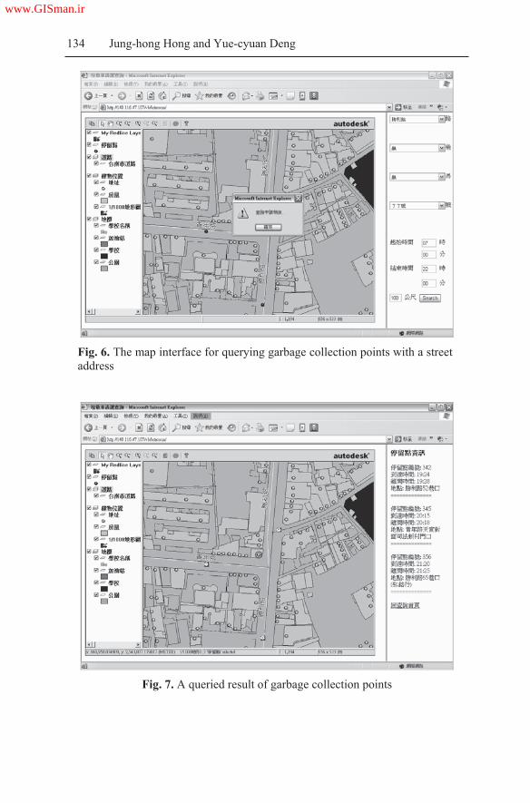
134 Jung-hong Hong and Yue-cyuan Deng

Fig. 6. The map interface for querying garbage collection points with a street

address

Fig. 7. A queried result of garbage collection points

www.GISman.ir

An Evaluation of GIS-aided Garbage Collection Service 135

3.2. An Evaluation of the Garbage Collection Service

There were altogether 71,246 households in the research area based on the

street address database provided by the city government. We analyzed the

serviceable areas for 895 garbage collection points using five different dis-

tance constraints: 50 meters, 75 meters, 100 meters, 125 meters and 150

meters. For every chosen distance constraint, we can determine the number

of accessible collection points for individual households and calculate the

total number of households on the basis of the number of accessible collec-

tion points (Table 1). For example, under the column of “50 meter” buffer,

“25,236” is interpreted as “there exists 25,236 households with zero acces-

sible collection points within 50 meters of their residence.” Similarly, 95

households have access to 4 garbage collection points. Some other findings

are discussed as follows:

1. It can be seen from Table 1 that the number of non-serviceable house-

holds decreased from 25,236 (35% of the total households) to 62 house-

holds (0.08%) with increasing buffer distances from 50 meters to 150

meters. Indeed, only about 2% of the households would remain non-

serviceable were the residents willing to walk 100 meters to the collec-

tion points.

Table 1. Statistics of the number of accessible collection points and the number of

households based on different distance buffers

50 m 75m 100m 125m 150m

0 25236 6894 1319 197 62

1 33494 24508 8834 3173 1117

2 11105 22569 16230 6907 3578

3 1496 12324 18812 9486 3505

4 95 3822 13501 14820 7258

5 1195 7989 12390 9246

6 103 3279 10438 11023

7 11 1067 7737 9989

8 311 3842 8071

9 75 1572 7005

10 6 622 4647

11 3 191 2901

12 31 2008

13 20 734

14 165

15 104

16 13

BufferNumber of

accessible collection points

www.GISman.ir

An Evaluation of GIS-aided Garbage Collection Service 137

Fig. 8. Number of serviceable households with different conditions

Fig.9. Number of households serviceable both before and after 6:30pm

Figure 9 shows the number of households serviceable both before and

after 6:30pm. This quantitative measure allows for an assessment of the

provision of garbage collection services. Even with the number of service-

able households steadily increasing as the distance buffer increases from

50 meters to 150 meters, only 26,125 qualified households (about 1/3 of

the total households) are served at the 100 meter distance buffer. Unless a

higher level of garbage collection service is expected both before and after

6:30pm by the majority of residents, the current schedule and configura-

tion of garbage collection points need no major modification.

www.GISman.ir

138 Jung-hong Hong and Yue-cyuan Deng

(a) 50 meters buffer (b) 75 meters buffer (c) 100 meters buffer

(d) 125 meters buffer (e) 150 meters buffer

Fig. 10. Spatial distribution of non-serviceable households based on different dis-

tance buffers

The above indicators provide overall measures about the “quality” of

garbage collection service. To improve the garbage collection service, the

most important thing is to identify non-serviceable households and adjust

collection routes and schedules accordingly. Figures 10 (a) - (e) illustrate

the spatial distribution of non-serviceable households assuming different

distance buffers. A 50 meter distance buffer yielded a widespread distribu-

tion of non-serviceable households which did not seem realistic. As the

distance buffer was increased, it became easier to identify “weak regions”

with non-serviceable households. Such maps are potentially useful in iden-

tifying areas needing more collection points. It should be noted that some

non-serviceable households are located close to the boundary of the east-

ern district, so they may be able to access garbage collection services pro-

vided by other districts. Figure 11 uses the thematic mapping technique to

illustrate the number of accessible collection points for individual house-

holds based on a distance buffer of 100 meters; the darker symbols indi-

www.GISman.ir

An Evaluation of GIS-aided Garbage Collection Service 139

cate the more accessible collection points a household has. From this fig-

ure, the authorities can see visually the levels of service provision.

Fig. 11. A thematic map illustration based on the number of accessible collection

points of individual households.

(a) 50 meters buffer (b) 100 meters buffer (c) 150 meters buffer

Fig. 12. A spatial distribution of non-serviceable households within the “building”

landuse districts

A critical factor for evaluating the garbage collection service for house-

holds located within the “building” landuse districts is its level of night-

time service provision. Figures 12 (a) - (c) illustrate the spatial distribution

of non-serviceable households after 6:30pm using three different distance

buffers. When the distance buffer is 50 meters, it is clear that the provision

level is rather poor. As the distance buffer increases, we can find a trend of

www.GISman.ir

140 Jung-hong Hong and Yue-cyuan Deng

spatial distribution similar to that of Figure 10. Since the non-serviceable

households are again located within a limited area, the addition of more

garbage collection points near these regions should be able to improve ef-

fectively the non-serviceable situations.

4 Conclusion

Garbage processing is a common challenge facing modern cities world-

wide. Major cities in Taiwan have adopted the “no garbage on the ground”

policy and relied on fixed-route and fixed-schedule trucks to collect gar-

bage. The success of such services is depended on a well-designed geo-

metric configuration of garbage collection points and careful planning of

the arrival times of garbage trucks. We successfully demonstrated in this

chapter the use of GIS in the evaluation of the level of service provision in

garbage collection. Compared with the traditional handbill approach, the

introduction of the WebGIS technology allows for ubiquitous access via

the Internet and an easier dissemination of garbage collection information.

Its flexible query capability further allows the search of all serviceable

garbage collection points within a selected neighborhood.

We further proposed four indicators to quantitatively measure the gar-

bage collection service based on the geometric distribution of households

and collection points. The use of a GIS offers powerful tools to calculate

indicator values and to undertake thematic mapping to illustrate the spatio-

temporal nature of the analyzed results. Our analyses indicated that the

proposed four indicators can highlight characteristics of a specific configu-

ration of garbage collection points, particularly in reference to require-

ments of the residents. Our example of the eastern district suggested that

the current configuration of collection points can provide sufficient ser-

vices to its residents at a distance buffer of 100 meters. Because the loca-

tions of non-serviceable households are displayed on maps, the authorities

are in a better position to adjust the routes and collection points to improve

the service level of the “weak regions.” For the garbage processing au-

thorities, a GIS is therefore not only an invaluable aid to bridging the gap

between the government and the general public, but also a powerful tool to

improving the level of service provision in garbage collection.

www.GISman.ir

An Evaluation of GIS-aided Garbage Collection Service 141

Acknowledgements

The authors would like to express their appreciation to the Healthy City

Research Centre of the National Cheng-Kung University for their assis-

tance in the preparation of this chapter. Some of the ideas and technology

used in this chapter are from the research result of an NSC sponsored re-

search project (NSC94-2211-E-006-071).

References

[1] Gatrell AC (1991) Concepts of Space and Geographic Data, In: Maguire DJ,

Goodchild MF, Rhind, DW (eds.) Geographical Information Systems, Vol-

ume 1: Principles, Longman Scientific & Technical, pp. 119-134

[2] Healthy City Research Centre (2005) White Paper for the Healthy City of the

Tainan City, National Cheng Kung University in Tainan, 116 pages

[3] Hu SC and Tsai SY (2004) Concepts of WHO Healthy Cities, Journal of

Healthy Cities, Taiwan, 1(1): 1-7

[4] Melnick AL (2003) Introduction to Geographic Information Systems in Public

Health. Aspen Publishers. Inc. 300 pages

[5] National Council for Sustainable Development (2006) Sustainable Develop-

ment Indicator System, http://www.cepd.gov.tw/sustainable-development/

eng/main.htm, Accessed on March 10, 2006

[6] Soret S, McCleary K, Rivers PA, Montgomery SB, Wiafe SA (2002) Under-

standing Health Disparities through Geographic Information Systems. In: W.

Khan (ed.) Geographic Information Systems and Health Applications, Idea

Group Publishing, pp. 12-42

[7] Su HY (2003) The Garbage Sampling and Analysis in Taiwan in 2002: Final

Report,

http://ivy2.epa.gov.tw/out web/twdep/www/d40/%E6%96%B0%E8%B3%87

%E6%96%99%E5%A4%BE/Chapter 2.pdf, Accessed on January 15, 2006

[8] TWNIC (2003) Broadband Network Use Survey Analysis in Taiwan, Taiwan

Network Information Centre, http://www.twnic.net.tw/file/TWNIC-Borband

Survey-92.08.19.pdf, Accessed on March 10, 2006

[9] Zheng YM (2000) “Current Status of Garbage Processing and Questions in

Taiwan.” http://eec.kta.org.tw/incinerator/diox111.htm, Accessed on March

15, 2006

www.GISman.ir

A Study of Air Quality Impacts on Upper

Respiratory Tract Diseases

Huey-hong Hsieha, Bing-fang Hwangb, Shin-jen Chenga and Yu-ming

Wangc

a Department of Environment and Resources Engineering, Diwan College

of Management, Taiwan b School and Graduate Institute of Occupational Safety and Health College

of Public Health, China Medical University, Taiwan c Department of Information Management, Diwan College of Management,

Taiwan

Abstract: Upper respiratory tract (URT) diseases are highly related to air

quality. Recent interests have focused on traffic-related air pollution and

the potential health effects associated with such exposure. These studies

have indicated a strong correlation between air pollution and its related

diseases. With advances made in computer technologies, Geographic In-

formation Systems (GIS) nowadays provide useful spatial analysis tools to

examine spatial characteristics of air quality. Maps of the spatial distribu-

tion of air pollutants can be produced with a GIS to facilitate in-depth stud-

ies. Our study incorporated the 2003 Cancer Death Rate (CDR) map pro-

vided by the Bureau of National Health Insurance with the air quality data

provided by the Environmental Protection Agency to examine the associa-

tions between air pollution and upper respiratory tract diseases. First, maps

of select air pollutants (NOX, O3, PM10, SO2 and CO) were produced using

the inverse distance weighting interpolation method. Then, a series of sta-

tistical analyses were performed to examine the correlation between these

pollutants. Finally, a multivariate regression analysis of association was

preformed to study the correlation between air pollution and URT diseases.

The results indicated a strong correlation between NOX and CO (coeffi-

cient of correlation 0.92), and association between these pollutants and

URT diseases.

Keywords: upper respiratory tract disease, air quality, multivariate re-

gression

www.GISman.ir

A Study of Air Quality Impacts on Upper Respiratory Tract Diseases 143

1 Introduction

Recent research from the U.S., Netherlands and Australia reported an as-

sociation between URT diseases and the air quality (Woolcock, et, al,

1997, Boezen, et al., 1999, Brunekreef, et al., 2002). In Taiwan, the rela-

tionship between the diseases and air quality has not yet been discussed.

Air pollutant exposure on an individual can be estimated from measure-

ments recorded by nearby monitoring gauges. However, air pollutants vary

in space and time and the gauge measurements only provide point-based

exposure values at an instance. To extend the point-based measurements of

air pollutant exposure, spatial interpolation was applied on these point

measurements using a GIS to estimate a pollution surface. Associative

analyses were then applied to find the relationships between the URT dis-

eases and the derived air pollutant values.

The procedures can help extract the most significant influential factors

of URT diseases. In addition, the derived air pollutant maps can provide

useful information for related analyses.

2 Data Characteristics

Three types of data sources were used for our analyses: (1) Air Quality

System (AQS) database from the Environment Protection Administration

(EPA), (2) Census database from the Department of Statistics of the Minis-

try of Interior (DSMI), and (3) the Cancer Distribution (CD) database pro-

vided by the Bureau of Health Promotion of the Department of Health

(BHPDH). The following sections describe in greater detail the character-

istics of each type of data.

2.1 Air Quality System (AQS) database

The AQS database contains measurements of air pollutant concentrations

in Taiwan under the provisions of the Clean Air Act intended to monitor

the quality of air. The EPA sets limits on the acceptable amounts of a

range of pollutants present in the air. Included in the measurements are the

five criteria air pollutants: Carbon Monoxide (CO), Nitrogen Dioxide

(NO2), Sulphur Dioxide (SO2), Ozone (O3), and Particulate Matter (PM10).

The air quality monitoring network of Taiwan consists of 58 gauges as il-

lustrated in Figure 1. The measurements of each pollutant were interpo-

lated into a pollution surface for further analyses.

www.GISman.ir

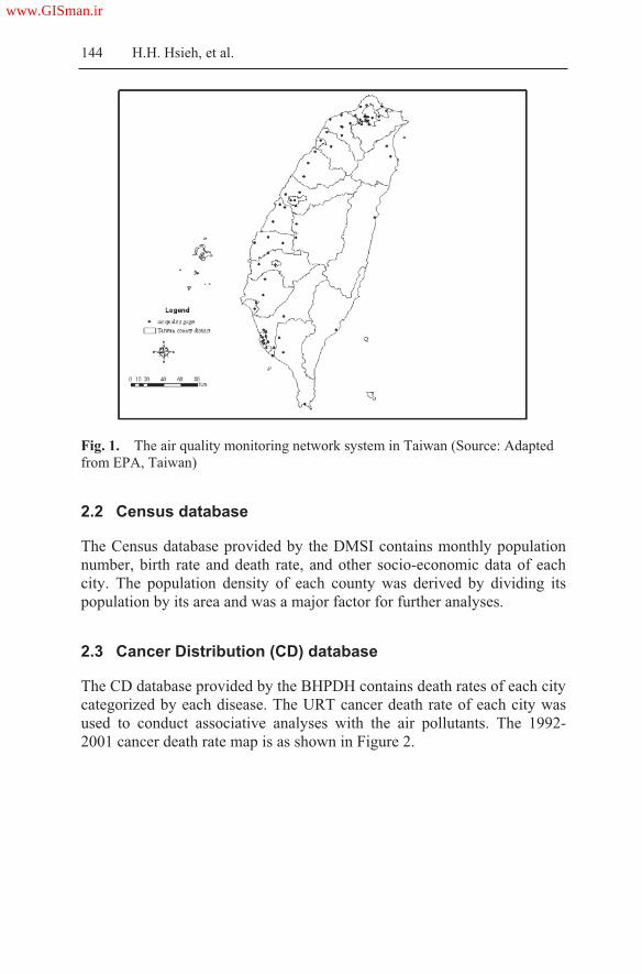
144 H.H. Hsieh, et al.

Fig. 1. The air quality monitoring network system in Taiwan (Source: Adapted

from EPA, Taiwan)

2.2 Census database

The Census database provided by the DMSI contains monthly population

number, birth rate and death rate, and other socio-economic data of each

city. The population density of each county was derived by dividing its

population by its area and was a major factor for further analyses.

2.3 Cancer Distribution (CD) database

The CD database provided by the BHPDH contains death rates of each city

categorized by each disease. The URT cancer death rate of each city was

used to conduct associative analyses with the air pollutants. The 1992-

2001 cancer death rate map is as shown in Figure 2.

www.GISman.ir

A Study of Air Quality Impacts on Upper Respiratory Tract Diseases 145

Fig. 2. Age-adjusted cancer mortality by precinct and township of Taiwan

(Source: Adapted from BHPDH, Taiwan)

3 Methodology

As introduced in the previous section, three types of data were used in this

study. Each data set was pre-processed for further analyses. Four proce-

dures were involved in the analyses: (1) interpolation of the point data, (2)

extraction of estimated values at specific locations on a surface map, (3)

analyses of the correlation between air pollutants, and (4) association

analyses between the URT diseases and air pollutants. The following sec-

tions briefly describe the processes.

3.1 Interpolation of point data

The air pollutant measurements from AQS database were integrated into

monthly and yearly point data and interpolated to pollutant surfaces using

the inverse distance weighting method. The method is briefly described as

below.

www.GISman.ir

146 H.H. Hsieh, et al.

Inverse distance weighting is the simplest interpolation method. A

neighborhood about the interpolated point is identified and a weighted av-

erage is taken of the observation values within this neighborhood. The

weights are a decreasing function of distance. The user has control over the

mathematical form of the weighting function, the size of the neighborhood

expressed as a radius or a number of points, in addition to other options

(Fisher, 1987). The weighting function is formulated as follows:

w(d)= 1/dp

where w(d) is the weighted distance;

d is the distance; and

p>0 is the weight

Eqn. (1)

The value of p is specified by the user. The most common choice is p=2.

When p=1, the interpolated function is "cone-like" in the vicinity of the

data points, where it is not differentiable. Shepard's (1968) method is a

variation of the inverse power, with two different weighting functions us-

ing two separate neighborhoods. The default weighting function for the

Shepard's method is an exponent of 2 in the inner neighborhood and an ex-

ponent of 4 in the outer neighborhood. The form of the outer function is

modified to preserve continuity at the boundary of the two neighborhoods.

The neighborhood size determines how many points are included in the in-

verse distance weighting. The neighborhood size can be specified in terms

of its radius (in km), a number of points, or a combination of the two. The

use of a radius requires the user to specify an override value in terms of a

minimum and/or maximum number of points. Invoking the override option

will expand or contract the circle as desired. Conversely, specification by

number of points requires an override value in terms of minimum and/or

maximum radius. It is also possible to specify an average radius as an

override to expand or contract the size of a neighborhood.

3.2 Extraction of estimated values at specific locations on a surface map

The air pollutant surfaces derived from the previous section summarize the

spatial distribution of each pollutant. To examine correlations among the

pollutants and possible association between these air pollutants and the

URT diseases, air pollutant readings at each URT disease locations were

extracted from the derived concentration surface maps. The ArcGIS Spa-

tial Analyst tool (developed by ESRI) was used to extract pollutant read-

ings at specified locations on a surface.

www.GISman.ir

A Study of Air Quality Impacts on Upper Respiratory Tract Diseases 147

3.3 Analyses of correlation between air pollutants

The correlation between a pair of air pollutants was calculated using the

Pearsons coefficient of correlation (Edwards, 1976) expressed as follows:

Eqn. (2)

where R is the correlation coefficient;

x and y are readings for pollutant x and pollutant y respectively; and

n is the number of measurements.

The correlation coefficient is between -1 and 1; with –1 and 1 indicating

perfect negative and positive correlation between variables in the sample

data and with a value of 0 indicating no relationship between the variables

in the sample data.

3.4 Association analysis between URT diseases and air pollutants

The relationships between the URT diseases and the air pollutants can be

assessed using the Kendall coefficient of concordance (Gibbons, 1997)

which indicates the degree of association between the variables in the

sample data. The test variables in ordinal measurement must be rearranged

before the Kendall coefficient of concordance can be calculated. The fol-

lowing sub-sections describe briefly the procedures.

3.4.1 Data ranking

Suppose the data consist of a random sample of n pairs of observations

with k variables, (X11, X21, X31, …, XK1), (X12, X22, X32, …, XK2),

…, (X1n, X2n, X3n, …, XKn), where each set (that is X1 set, X2 set,

…, XK set) is measured on an ordinal scale. For the purpose of the analy-

sis, observations in each set are ranked. That is, the integers 1,2,3, …, n

are assigned to X11, X12, X13 according to their relative magnitudes

within the set of X1 observations. Let U1i denotes the rank of X1i, so the

set U11, U12, …, U1n represents some arrangement of the first n positive

integers. Similarly, the series of Xk1, Xk2, Xk3, …, Xkn is ranked; the re-

sults of this ranking are denoted by Uk1, Uk2, …, Ukn. Now the data to be

analyzed consist of n pairs of positive integers (U11, U21, …, Uk1), …,

(U1n, U2n, …, Ukn), which represent the pairs of ranks of the original ob-

servations. In the discussion to follow, we assume for convenience that

2222 yynxxn

yxxynR

www.GISman.ir

148 H.H. Hsieh, et al.

these pairs are listed in increasing order of the value of the Xk ranks; that

is Uki=I, for i=1,2, …, n.

3.4.2 Rationale for the descriptive measure

The rankings of the k characteristics are in perfect agreement if and only if

U1i=U2i= … =Uki for each i. The rankings of the k data characteristics are

in perfect disagreement if they are paired in completely reverse orders.

3.4.3 Kendall coefficient of concordance for complete rankings

As mentioned in section 3.4.1, suppose the data consist of k complete sets

of rankings of n objects. Each ranking is made by a comparison of objects

within the set only. The data as collected or observed consist of nk ranks or

measurements on at least an ordinal scale. The rankings are assigned sepa-

rately within each of the k group. The association between the k sets of

rankings is of interest. For simplicity, the ranks of each set are assigned

accordingly. The sum of ranks from X11, X12, …, X1n to Xk1, Xk2, …,

Xkn are calculated accordingly. We use S1, S2, …, Sk to denote the sum

of ranks for each set. The sum of ranks of each data set is also calculated

and is summarized in total Sk. Let Sa denote the average of a perfect

agreement of data sets, then Sa=Sk/n. If data sets are in perfect agreement,

then S1=S2=… =Sk. Let S denotes the sum of squares of deviations be-

tween the observed sums and the expected sums, as expressed in the fol-

lowing form:

S=(S1-Sa)2+(S2-Sa)2+ … + (Sx-Sa)2

If the k sets of rankings are in perfect agreement, the rank of X11, X12,

…, X1n will be assigned rank 1 and the sum will be n. The sum of ranks of

X21, X22, …, X2n will have a value of 2n, and so forth. We can then cal-

culate the sum Sd of squares of deviations of these column sums (with per-

fect agreement) from the column expected (with no association):

Sd=(n-S)2+(2n-S)2+…+(n2-S)3= [Sj-k(n+1)/2]2 Eqn. (3)

where j=1,2, …, n

The relative agreement can be measured by a ratio of the actual sum of

squares to the sum of squares under a perfect agreement, or

W=Sd/Sa=12Sd/k2n(n2-1)

where W denotes the Kendall coefficient of concordance.

www.GISman.ir

A Study of Air Quality Impacts on Upper Respiratory Tract Diseases 149

The ratio will clearly compute to 1 for a perfect agreement and tend to-

ward 0 for no agreement.

3.4.5 Test of association

Given that the k sets of rankings result from measurements on k character-

istics, the Kendall coefficient of concordance can be used to test the null

hypothesis that these characteristics are independent. In other words, there

is no association or relationship between the k variables. The hypothesis is

set as below:

HO: No association HA: Association exists

The p-value or significance level is the right tail and can be determined

from a reference table of the Kendall coefficient of concordance. A 95 per-

cent confidence interval or 0.05 significance is used for the test.

3.5 Analysis procedures

The analysis procedures are outlined in the following steps:

Step 1: Find the URT death rate for each city from the CD database

Step 2: Transfer the death rate into a geodatabase

Step 3: Interpolate the point-based URT death rate data into a surface

Step 4: Extract from the surface derived in step 3 death rate values at

the EPA questionnaire locations

Step 5: Interpolate the point-based air pollutant data of CO, NOx, SO2,

O3, PM10 into surfaces

Step 6: Extract from surfaces derived in step 5 values of pollutants at

the EPA questionnaire locations

Step 7: Find population density values at the EPA questionnaire loca-

tions

Step 8: Examine correlation between air pollutants

Step 9: Examine correlation between URT death rate and population

density

Step 10: Test for association between URT death rate and air pollutant

values

www.GISman.ir

150 H.H. Hsieh, et al.

4 Results

The analyses were performed following the procedures mentioned in sec-

tion 3 and the results presented below.

4.1 Spatial distribution of air pollutants

The study first computed the 1996 yearly concentration of air pollutants

from the AQS database. These point-based data were then interpolated into

concentration surfaces as shown in Figure 3. Note that the mountainous

area in the middle was removed from the analysis since there were no

monitoring gauges in this area.

Fig. 3. 1996 yearly air pollutant distribution and population density (figures from

upper left to right, then lower left to right show the concentration of CO, NOx,

SO2, O3, PM10, and population density)

www.GISman.ir

A Study of Air Quality Impacts on Upper Respiratory Tract Diseases 151

pollutant NOx O3 PM10 SO2 CO

NOx 1.00 -0.47 0.04 0.32 0.92

O3 -0.47 1.00 0.26 -0.11 -0.47

PM10 0.04 0.26 1.00 0.51 0.26

SO2 0.32 -0.11 0.51 1.00 0.51

CO 0.92 -0.47 0.26 0.51 1.00

From the series of surface maps, we could see that pollution was more

serious in the urban areas such as Taipei and Kaoshung. Southern Taiwan,

however, registered a more serious level of air particulate suspension of

PM10 than the north, possibly a result of uneven rainy days. In the northern

part, the rainy season was longer than the central and southern parts of Tai-

wan during the study period and rain was suspected to wash away sus-

pended particulates.

Table 1. Correlation coefficients between air pollutants

The correlation between the various air pollutants were calculated and

shown in Table 1 which shows a strong relationship between NOx and CO

with a correlation coefficient of 0.92. Hence, one of the two pollutants

needed to be excluded from the associative analysis between URT death

rate and air pollutants. In the study, CO was removed from the analyses of

association. Also SO2 and CO are correlated (R = 0.51) and there exists a

reverse correlation between NOx and O3 (R = –0.47).

4.3 Correlation between URT death rate and air pollutants

The correlation coefficient of the URT death rate and population density

was 0.1, which indicates a weak relationship between them. The correla-

tion coefficients between the URT death rate and NOx, O3, PM10, SO2 and

CO were: 0.26, -0.09, 0.03, 0.26, 0.25 respectively. These results indicate

positive although weak relationships between the URT death rate and

NOx, SO2 and CO.

4.4 Associative analysis

Given the weak correlation between the URT death rate and NOx, SO2 and

CO, these three pollutants were taken into further consideration for asso-

ciative analysis with the URT death rate.

www.GISman.ir

152 H.H. Hsieh, et al.

The test was performed in SPSS and the test statistics was 0.9 with a p

value of near 0 indicating rejection of the null hypothesis. This result im-

plies that a strong association of the URT diseases and the pollutants.

5 Summary and suggestions

This study combined three types of data in an analysis of pollutants and

their possible effects on the URT diseases. Point-based data on pollutants

were used to derive air pollutant surfaces which facilitated the study of the

relationships between the UTR diseases and various air pollutants. Major

findings are summarized below:

1. The correlation coefficients between air pollutants indicated a strong re-

lationship between NOx and CO and moderate correlation between O3

and CO.

2. The UTR diseases and population density were not correlated.

3. The UTR diseases and the air pollutants (NOx, SO2, and CO) exhibited

a strong association.

Suggestions for further analyses include a more refined examination of

air pollutant concentrations and other factors leading to pollution, such as

vehicle emissions. The monthly or daily air pollutant concentrations may

be used to examine in greater detail occurrences of the UTR diseases. Ve-

hicle emission data may be obtained from the transportation fluxes data-

base to further the understanding of the UTR diseases and air quality.

Acknowledgements

The authors would like to thank the Environment Protection Administra-

tion, Department of Statistics, Ministry of Interior, and the Bureau of

Health Promotion of the Department of Health for the provision of data for

this study. Thanks also go to the National Science Council for the funding

of this research (project no. NSC932320-B-434-001).

References

[1] Boezen HM, Van der Zee SC, Postman DS, et al. (1999) Effect of ambient air

pollution on upper and lower respiratory symptoms and peak expiratory flow

in children. Lancet 1999; 353:874-878

www.GISman.ir

A Study of Air Quality Impacts on Upper Respiratory Tract Diseases 153

[2] Brunekreef B (2002) Particulate matter and lung function growth in children:

a 3-yr follow-up study in Austrian schoolchildren (correspondence). Eur Res-

pir J 2002; 20:1354-1355

[3] Edwards AL (2002) The Correlation Coefficient. In: An Introduction to Lin-

ear Regression and Correlation. San Francisco, CA: W. H. Freeman, Ch4, pp.

33-46, 1976

[4] Fisher NI, Lewis T, Embleton BJJ (1987) Statistical Analysis of Spherical

Data, Cambridge University Press, pp 329

[5] Gibbons JD (1997) Nonparametric Methods for Quantitative Analysis,

American Science Press, pp 537

[6] Shepard D (1968) A two-dimensional interpolation function for irregularly-

spaced data, Proc. 23rd National Conference ACM, ACM, pp 517-524

[7] Woolcock AJ and Peak JK (1997) Evidence for the increase in asthma world-

wide, Ciba Found Symp., p 206:122-134

www.GISman.ir

Spatial Epidemiology of Asthma in Hong Kong

Franklin F.M. Soa and P.C. Lai b

a Experian Asia Pacific, Experian Limited b Department of Geography, The University of Hong Kong

Abstract: This chapter employs Geographic Information Systems (GIS) in

a study of asthma, a major respiratory disease in Hong Kong. Hospital ad-

missions records for the period 1996-2000 were obtained from the Hong

Kong Hospital Authority. Residential addresses of patients were geocoded

in a GIS and aggregated to make reference to the demographic statistics in

census enumeration units. Disease maps were used to explore the relation-

ship between the Standardized Morbidity Ratio (SMR) and three environ-

mental factors of population density, land use, and air pollution. A strong

positive correlation was found between asthma incidence and high-density

residential areas and industrial development. A lack of direct association

between asthma admissions and air pollution indicates that the relationship

may not be that explicit from the spatial context.

Keywords: geographic information system, GIS, respiratory disease,

asthma, spatial epidemiology, Hong Kong

1 Introduction

The prevalence of asthma1 is increasing worldwide (WHO 2000; Wieringa

et al., 2001; Corburn et al., 2006). The WHO (2000) estimated that about

100- 150 million people around the world were suffering from asthma and

that the economic cost exceeded those of tuberculosis and HIV/AIDS

combined. Asthma epidemiology reported by the medical and clinical pro-

fession has always emphasized individual and family-based risk factors

1 Asthma is a disease characterized by recurrent attacks of breathlessness and

wheezing. This condition is due to inflammation of the air passages in the lungs

that affects the sensitivity of the nerve endings in the airways so they become

easily irritated. In an attack, the lining of the passages swell causing the airways

to narrow thereby reducing the flow of air in and out of the lungs (WHO,

2000).

www.GISman.ir

Spatial Epidemiology of Asthma in Hong Kong 155

such as indoor allergen exposures, tobacco smoking, and chemical irritants

(Clark et al., 1992; Richard et al., 2000; Skoner, 2001). A number of epi-

demiological studies also identified air pollution as another risk factor

(Schwartz, 1993; Koenig, 1999; Swift and Foster, 1999; Donaldson, et al.,

2000; Samet et al., 2004).

Spatial epidemiology, which describes and identifies spatial variations

in disease risks through map visualization and exploratory analysis, repre-

sents a new frontier of epidemiological research (Elliott et al., 2000;

Berke, 2005; Ostfeld et al., 2005). The spatial context facilitates a close-up

examination of diseases against their surrounding and neighborhood envi-

ronmental exposures (Corburn et al., 2006). The approach provides a way

to examine another spectrum of risk factors yet to be explored from the

clinical perspective (Meade and Erickson, 2000; Jackson, 2003; Fritz and

Herbarth, 2004; Kimes, et al., 2004; Oyana, et al., 2004). Advances in

digital technologies have facilitated the use of Geographic Information

Systems (GIS) in undertaking spatial epidemiological research (Ostfeld et

al., 2005). GIS is a tool to input, store, retrieve, manipulate, analyze and

output geographic or mappable data (Marble and Peuquet, 1983; DeMers,

1997). It facilitates three levels of analyses: (i) visual - to locate and plot

disease cases, (ii) spatiotemporal – to integrate and link cases and envi-

ronmental features in space and time, and (iii) geostatistical – to evaluate

the disease pattern by means of spatial and statistical inference.

The limited number of spatial epidemiological studies in Hong Kong

definitely underscores research gaps in this region. Applications of geo-

graphic concepts and techniques to health studies in Hong Kong came to

exist only in the mid-1990s with the first series of medical maps presenting

spatial patterns of malignant disease mortalities between 1979 and 1993

(Lloyd et al., 1996). These research studies mainly employed visual dis-

play and map presentation but with limited data manipulation and analyti-

cal capabilities (Lloyd, et al. 1996; Wong, et al., 1999). It was not until re-

cently in the 21st century that disease patterns in Hong Kong were analyzed

from the spatial perspective (So, 2002; Lai, et al., 2004).

Spatial epidemiological studies in Asian countries are comparatively

fewer in number and not as methodologically advanced as those of the

western world. While some studies conducted in the United States and

other developed nations have suggested that urban areas contribute more to

asthma, this observation is not evident in Hong Kong. It is believed that

there is much room for exploring the use of GIS in spatial epidemiological

studies of Hong Kong. The objectives of this chapter are twofold: (i) to

visualize the spatial distribution of asthma, and (ii) to examine the spatial

association of asthma occurrence against three environmental risk factors

namely, population density, land use, and air pollution. Essentially, resi-

www.GISman.ir

156 Franklin F.M. So and P.C. Lai

dential addresses of patients were mapped to represent disease events as

points which were then studied against other geographic data, such as air

pollution and land use surfaces. Likewise, the analysis was approached at

the neighborhood level using the census subdivision of Tertiary Planning

Units (TPUs) to present population density.

2 Methodology

Hong Kong (22º15’N, 114º10’E) bordering the South China Sea in East

Asia, is a densely populated city of 6.9 million occupying a total land area

of 1,098 square kilometers (Census and Statistics Department, 2000, p.

346). The population density in 2004 was 15 and 40 times more than Japan

and China respectively (Central Intelligence Agency, 2005). Respiratory

diseases were amongst the top-three killer diseases in Hong Kong (Hospi-

tal Authority, 2000, p. 10), with a cumulative death rate of over 90 per

100,000 population between 1996 and 1999. A sharp increase was evident

in hospital admissions of respiratory illness which nearly doubled in ten

years from 61,000 in 1988 to 118,000 in 1998 (Hospital Authority, 1999,

p. 19).

The 1996-2000 admission records of 44 public hospitals under the man-

agement of the Hospital Authority formed the primary data source of this

study. Records of private hospitals were not included because of inconsis-

tencies in the data collection and record keeping protocols. Moreover, pub-

lic hospital records accounted for over 80 percent of disease cases in Hong

Kong (Hospital Authority, 2000, p. 67). Each record contains a patient’s

age, gender, residential address, disease code according to the International

Code of Disease Version 9 (ICD-9 code), and dates of admission and dis-

charge. The address data provide crucial information to link the home lo-

cations of patients, while age and gender enable further breakdowns of pa-

tients into subgroups. The study was also confined to patients discharged

with asthma (ICD code = 493). A patient admitted repeatedly into hospi-

tals with the same disease and within the study period of 1996-2000 was

counted only in the first occurrence. The total records amounted to 52,020

admissions after having removed 754 repeat admissions of the same per-

son (representing 1.13% of total) and discounting the 1,609 cases, or 3% of

patients, with problem addresses.

The life expectancy of females in Hong Kong was 84.6 compared to

78.4 for males (Hospital Authority, 2003). It was found necessary to stan-

dardize the crude rates by gender and age groups to account for age-sex

difference in disease impacts. The Standardized Morbidity Ratio (SMR in

www.GISman.ir

Spatial Epidemiology of Asthma in Hong Kong 157

Eqn. 1) was employed to compute ratios of the at-risk population in an

area by comparing the observed number of patients against the expected

counts of various age groups by gender.

SMR = N

Rsi Pi

Eqn. (1)

where N = total number of patients in the observed population

Rsi = age-gender specific morbidity rate of age-gender interval i in the

standard population

Pi = the population of age-gender interval i in the observed population

The SMR measure expresses the difference between morbidity experi-

ence of the population under study and the experience of that population as

it would be if it experienced the age-specific rates of the comparison popu-

lation. A ratio of greater than 1.0 indicates greater than expected morbidity

has occurred while less than 1.0 indicates lower than expected morbidity.

The decimal fraction shows the percentage comparison. An SMR of 1.12,

for example, infers 12% more than the expected number of patients has

occurred.

GIS was employed to geocode the residential addresses by assigning

data items to some locations or geographic positions in Earth space

(Croner et al., 1996). However, address entries must first be standardized

to eliminate inconsistencies (such as mis-spellings or incomplete records)

since the patients were not provided with guidelines or rules in entering

their addresses. It was possible to geocode about 89.3 percent of the raw

records without much difficulty and painstakingly geocode 7.5 percent of

the records by interactive means, which required substantial manual inputs.

The remaining 3 percent of addresses could not be geocoded either be-

cause of missing details or incorrect entries of non-existing streets or

buildings.

Maps were employed to visualize spatial patterns of asthma using the

ArcGIS 9.1 software. Geocoded point data derived from address matching

formed the essential data for further analysis. Three levels of mapping and

spatial analyses were undertaken: point, Tertiary Planning Unit2 (TPU),

and District3. While point data can reveal raw distributional patterns, com-

2 Tertiary Planning Unit (TPU) is a census enumeration unit demarcated by the

Planning Department for the territory of Hong Kong. Each TPU is sub-divided

into a number of Street Blocks (SB) for urban areas and Village Clusters (VC)

for rural areas. 3 There are at present 18 districts in Hong Kong, 9 in the urban areas and 9 in the

New Territories, including Central and Western, Eastern, Islands, Kowloon

City, Kwai Tsing, Kwun Tong, Northern, Sai Kung, Sham Shui Po, Shatin,

www.GISman.ir

158 Franklin F.M. So and P.C. Lai

parison of these data with demographic statistics must be made in refer-

ence to census enumeration units by TPUs and Districts. The point data

were therefore aggregated by areal units using the point-in-polygon opera-

tion in a GIS to enable the making of thematic maps (Gatrell, 2002, p. 51).

This study employed the 2001 population census data of 139 TPUs as de-

fined by the Census and Statistics Department for finer comparison and 18

districts as defined by the District Council for territorial-wide analysis.

GIS was employed to facilitate the point-in-polygon and polygon-on-

polygon overlay operations. The geocoded point data were overlaid in a

GIS to examine variation of the SMR of asthma by the 18 Districts and

139 TPUs of Hong Kong. Analysis at the District level provides a general

overview, and more detailed spatial variations are reflected at the TPU

level. It was postulated that asthma occurrences are associated with popu-

lation density and land use types. The polygon-on-polygon overlay opera-

tion was used to examine the association of SMR of each district and TPU

against the population density as well as the land use patterns defined by

the Planning Department.

The association between asthma and air pollution was analyzed. Air pol-

lution data of Hong Kong were derived from a total of 14 monitoring sites

that measure, on a daily basis in Hong Kong since 1999, concentrations of

major pollutants, including the ambient respirable suspended particulate,

sulphur dioxide, carbon monoxide, ozone and nitrogen dioxide (Environ-

mental Protection Department, 2002). The Air Pollution Index (API)

summarizes the severity of the pollution level and is calculated by compar-

ing the measured concentrations of major air pollutants against their re-

spective health related Air Quality Objectives established under the Air

Pollution Control Ordinance. The mean seasonal API values were calcu-

lated for the 14 sites and the Inverse Distance Weighting (IDW) method

(Chung and Yun, 2004) used to simulate a grid-based air pollution surface

for each of the four seasons. Monthly hospital admission rates of asthma

patients for each district were regrouped to reflect seasonal changes and

these were compared against the overall average (i.e. annual average ad-

mission rate). Seasonal variations of asthma admissions of each district

were reduced to percentages above or below the overall average. These

seasonal figures were mapped against the API surfaces for the respective

seasons and their correlation coefficients computed.

Statistical methods were used to account for association between asthma

and three environmental variables of population density, types of land use,

and air pollution. The distribution of asthma was assumed to have a Pois-

Southern, Tai Po, Tsuen Wan, Tuen Mun, Wan Chai, Wong Tai Sin, Yau Tsim

Mong, and Yuen Long.

www.GISman.ir

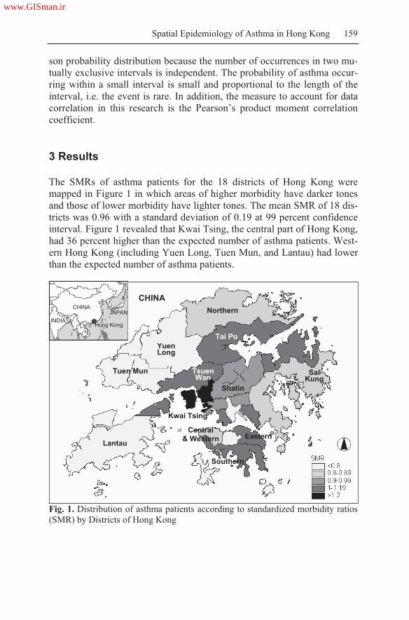
Spatial Epidemiology of Asthma in Hong Kong 159

son probability distribution because the number of occurrences in two mu-

tually exclusive intervals is independent. The probability of asthma occur-

ring within a small interval is small and proportional to the length of the

interval, i.e. the event is rare. In addition, the measure to account for data

correlation in this research is the Pearson’s product moment correlation

coefficient.

3 Results

The SMRs of asthma patients for the 18 districts of Hong Kong were

mapped in Figure 1 in which areas of higher morbidity have darker tones

and those of lower morbidity have lighter tones. The mean SMR of 18 dis-

tricts was 0.96 with a standard deviation of 0.19 at 99 percent confidence

interval. Figure 1 revealed that Kwai Tsing, the central part of Hong Kong,

had 36 percent higher than the expected number of asthma patients. West-

ern Hong Kong (including Yuen Long, Tuen Mun, and Lantau) had lower

than the expected number of asthma patients.

Fig. 1. Distribution of asthma patients according to standardized morbidity ratios

(SMR) by Districts of Hong Kong

CHINA JAPAN

INDIA Hong Kong

YuenLong

Tuen Mun

CHINA

Lantau

Tai Po

Tsuen Wan

SaiKung

Shatin

Central& Western

Kwai Tsing

Northern

Southern

Eastern

www.GISman.ir

160 Franklin F.M. So and P.C. Lai

SMR values were correlated against population density at the district

and TPU levels (Table 1). The district level analysis indicated a positive

but marginally insignificant (close to 90 percent confidence level) correla-

tion between disease morbidity and population density (r=0.329, p=0.103).

Given that the maximum plot ratio (i.e. Gross Floor Area / Population

Number) varies for different land use types, SMRs were further correlated

with densities of different land uses (classified as high-, medium- and low-

residential, and industrial in accordance with the statutory land use plan-

ning put forth by the Planning Department). Although not statistically sig-

nificant, it was interesting to note that SMR correlated positively with

high-density residential development (r=0.178) and negatively with low-

density residential development (r=-0.094). The above results warranted

more detailed examination at the TPU level.

Table 1. Correlation coefficients of SMR against population density and land use

types

Districts Tertiary Planning Units

All1

(N 18)

All1

(N 139)

HK2

(N 37)

KLN3

(N 44)

NT4

(N 58)

(a) Population density5 0.329+ 0.174* 0.149+ 0.127 0.262*

(b) High residential usage6 0.178 0.230** 0.230+ 0.237+ 0.270

(c) Medium residential us-

age7-0.031+ -0.387** -0.499** -0.351** -0.242+

(d) Low residential usage8 -0.094 -0.405** -0.488** -0.364** -0.434**

(e) Industrial usage9 0.064 0.227**0.278 0.208* 0.318**

+p < 0.10,

* p<0.05,

**p<0.01

Data Source: Hong Kong Hospital Authority 1996 2000; Hong Kong Census and Statistics Depart

ment 2001; Hong Kong Planning Department.

Note: 1 All areas covered by 18 Districts or 139 Tertiary Planning Units

2 HK Hong Kong Island

3 KLN Kowloon Peninsula

4 NT New Territories

5 Population density Number of 2001 population / Area

6 High residential usage High residential usage area / Total area; Indicates areas of

high density development and where commercial uses are always permitted on the

lowest three floors of a building or in the purpose designed non residential portion of

an existing building

7 Medium residential usage Medium residential usage area / Total area; Indicates ar

eas primarily used for medium density residential development

8 Low residential usage Low residential usage area / Total area; Indicates areas pri

marily intended for low rise and low density residential development

9 Industrial usage Industrial usage area / Total area; Indicates areas intended primar

ily for general industrial uses to ensure an adequate supply of industrial floor space to

meet demand from

Mapping of SMRs and correlation analyses at the TPU level were much

more revealing than the generalized district-based statistics. Figure 2

www.GISman.ir

Spatial Epidemiology of Asthma in Hong Kong 161

showed much variation in the SMR readings by TPUs in each of the 18

districts. The mean SMR value of 139 TPUs was 0.92, with a standard de-

viation of 0.32 at 95 percent confidence interval. It was also interesting to

note that while the mean SMR of three geographic constituencies (2a -

Hong Kong Island, 2b - Kowloon Peninsula, and 2c - New Territories)

were similar, SMR values of TPUs in Hong Kong Island varied much

more (standard deviation of 0.4) than for the Kowloon Peninsula and New

Territories (with standard deviations of 0.28 and 0.29 respectively). Be-

sides Kwai Tsing which registered a high SMR (at both district and TPU

levels), there were actually a few TPUs with high SMRs in Hong Kong Is-

land and the Kowloon Peninsula. Details rendered through TPUs (Figure

2) seem superior to those of Districts (Figure 1) in revealing the spatial

variation of disease morbidity.

N Mean StandardDeviation

Confidence Interval

N Mean StandardDeviation

Confidence Interval

37 0.90 0.40 ± 0.13 44 0.97 0.28 ± 0.08

N Mean StandardDeviation

Confidence Interval

N Mean StandardDeviation

Confidence Interval

58 0.91 0.29 ± 0.08 139 0.92 0.32 ± 0.05

Note: 3a Hong Kong Island; 3b Kowloon Peninsula; 3c New Territories

Data Source: Hospital Authority 1996 2000; Census and Statistics 2001.

Fig. 2. Distribution of asthma patients according to standardized morbidity ratios

(SMR) by Tertiary Planning Units of Hong Kong

2a 2b

2c

2b

2a

2c

www.GISman.ir

162 Franklin F.M. So and P.C. Lai

Table 1 presents correlation values broken down by three geographic

constituencies in comparison to the whole of Hong Kong. There is a clear

indication of a statistically significant correlation between SMR and popu-

lation density in Hong Kong (r=0.174, p<0.05). Further analyses broken

down by land use types indicated positive correlation with high-density

residential and industrial development (r=0.23, p<0.01 and r=0.227,

p<0.01) and negative correlation with medium- and low- density residen-

tial development (r=-0.387, p<0.01 and r= -0.405, p <0.01), all of which

were statistically significant at the 99 percent confidence interval. Interest-

ingly, the geographic constituencies contributed in varying degrees to the

highly significant relationships in each land use types. In particular, the

negative correlation between SMR or asthma morbidity and low-density

residential development was significant in all three geographic constituen-

cies.

The attempt to examine the possible association between asthma and air

pollution from the spatial perspective was rather illuminating. The effects

of seasonal variations of air quality on asthma admissions were summa-

rized in Figure 3. Areas colored in dark brown or grey (Figures 3a, 3c and

3d) indicated the worsening of air pollution while light and dark green

tones (Figure 3b) represent lower APIs. Air pollution in Hong Kong was

worst in the winter and acceptable in the summer months. The maps also

underscored northern Wan Chai as the pollution black spot in Hong Kong.

At first glance, Figure 3d revealed that adverse atmospheric conditions in

the winter had a parallel effect on asthma admissions. However, the high-

est APIs were recorded in Eastern, Central and Western districts of the

Hong Kong Island and Yau Tsim Mong in the Kowloon Peninsula but the

greatest increase in admissions was not reflected in these districts (as evi-

dent from the directions and sizes of arrows). This lack of direct associa-

tion seemed to indicate that the relationship between asthma admissions

and air pollution might not be explicit.

Further analyses using the Pearson’s correlation coefficients highlighted

seasonal variations between APIs and asthma admissions (Figure 4). Al-

though the winter and summer months respectively recorded consistently

high or low pollution levels, the range of values was not as widespread.

Statistical results did not indicate a significant relationship between the

APIs and asthma admissions in these seasons. The relationship between

asthma admission rates against generalized APIs was significant and posi-

tive for spring (r=0.534, p<0.01) but negative for autumn (r=-0.581,

p<0.01). It is suspected that unstable air currents brought about by the

monsoons in autumn contributed to this lack of association. The overall

plot however clearly indicates a positive relationship with statistical sig-

nificance (r=0.652, p<0.01).

www.GISman.ir

Spatial Epidemiology of Asthma in Hong Kong 163

(a) Spring (b) Summer

(c) Autumn

Seasonal variation of asthmaadmissions was apparent from variation in the sizes and directions of the arrows. Deviations in asthmaadmissions comparedagainst the overall average were plotted on four air pollution surfaces, each representing the air pollution levels derived from API readings for the respective seasons.

The effects of air pollutants were derived from API readings from the Environment Protection Department.

(d) Winter

Fig. 3. Effects of seasonal variations of air quality on asthma admissions in

Hong Kong, 1996-2000

Decrease by >20%

Decrease by 16 20%

Decrease by 11 15%

Decrease by 6 10%

Decrease by 1 5%

Increase by 1 5%

Increase by 6 10%

Increase by 11 15%

Increase by 16 20%

Increase by >20%

www.GISman.ir

164 Franklin F.M. So and P.C. Lai

30

20

10

0

10

20

30

20 25 30 35 40 45 50 55 60 65 70 75 80

Air Pollution Index (API)

Hospta

Adm

ss

on (

%)

Spring

Summer

Autumn

Winter

Time Interval Statistical significance, two-tailed: *p<0.01

Spring (Mar - May) 0.534*

Summer (Jun - Aug) 0.274

Autumn (Sep - Nov) -0.581*

Winter (Dec - Feb) -0.296

All seasons 0.652*

The relationship between deviations

in asthma admissions against the

generalized APIs was significant and

positive for spring and negative for

autumn. Admission: Percent of hospital admissions of asthma cases above or below the average, 1996 2000.

API: Generalized Air Pollution Indices sourced from the 14 monitoring sites in 1999 and 2000.

Data Source: Hospital Authority 1996 2000; Environmental Protection Department 1999 2000.

Fig. 4. Graphic plots of deviations in asthma admissions against seasonal air pol-

lution indices of Hong Kong, 1996-2000

4 Discussion

This research has demonstrated the use of GIS in a spatial epidemiol-

ogical study of asthma in Hong Kong making use of disease maps to ex-

amine the causative relationship between asthma and environmental risk

factors, i.e. population density, land use, and air pollution. This study is the

first attempt in Hong Kong to use hospital morbidity data with patient ad-

dresses, particularly down to individual building blocks, to geocode and

(

www.GISman.ir

Spatial Epidemiology of Asthma in Hong Kong 165

analyze patterns of diseases in a GIS. While the approach of point mapping

that displays residential locations of patients has raised concerns regarding

privacy and confidentiality of health records (Rushton, 1998), the avail-

ability of such data enables nested case-control or case-cohort study to be

conducted for direct study within a large-scale population based cohort

(Diggle, 2003; Elliott and Wartenberg, 2004). Point mapping at the initial

stage was adopted to compile area-based statistics by district and TPU. It

was shown that data summarized by 139 TPUs provided sufficient detail to

characterize spatial variation of disease morbidity.

The use of exact address location as the data unit may also lead to the

problem of epidemiological inference (Lawson, 2001) because a case ad-

dress used to represent residential exposure to environmental risk may not

be comprehensive enough to reflect the individual exposure occurring at

work, at school, or at regular weekend visits (Wakefield, et al., 2001).

Given that technologies can handle very detailed accounts of human activi-

ties, the question of how far ‘society’ wants to go in the use of personal

data to increase our understanding of disease, and exposure, must be

posed. Considering all of the above, mapping by patient addresses is an

acceptable and practical option.

The flexibility to partition data sets by various levels of detail by auto-

mated means in a GIS has greatly extended our ability to probe spatial

data. Users of GIS, however, must take time to examine the input data and

make necessary adjustments to the data before further analysis. Various

cartographic and geo-statistical techniques were employed to enhance un-

derstanding of the spatial event. Some cartographic presentations shown in

this research are experimental in nature as they have not been attempted by

other researchers. The air pollution surfaces were interpolated and extrapo-

lated from APIs recorded from 14 monitoring stations. Despite extensive

epidemiological evidence of the adverse effect of air pollution on asthma,

this study did not reveal a direct association, perhaps due to the sparseness

of the API data points. Although mobile air pollution monitoring platforms

have been developed to supplement the fixed number of monitoring sites

(Department of Chemical Engineering HKUST, 2002), this study did not

have access to these data. Other contributing factors of air pollution (such

as terrain, wind, and traffic) were not accounted for in this study. The rela-

tionship between these risk factors can also be further examined in the

three-dimensional (3D) modeling environment of a GIS. For instance, the

relationship between respiratory diseases and the ventilation of air condi-

tioning systems in offices or buildings can be investigated in 3D. This

method would be particularly valuable in Hong Kong because of its hilly

terrain and the abundance of high-rise buildings. The topographic effect of

www.GISman.ir

166 Franklin F.M. So and P.C. Lai

air pollution, wind direction, and wind speed on the distribution of disease

patients should also be investigated in the future.

The feasibility of the approach was largely dependent on the data qual-

ity. It should be noted that there were quite a number of data problems in

conducting this study. Attempts were made to resolve these issues in a sat-

isfactory manner, but some of the problems would never have arisen had

certain data been included in the process of data collection. First, given

that our study employed primarily secondary data sources, some issues on

data availability and comparability were unavoidable. In addition, patient

data of this research originated from admission records of public hospitals

under the management of the Hospital Authority. Similar data of private

hospitals, or clinics other than hospitals, were not included in this study

because of data inconsistency and resource constraints. It is arguable that

the incomplete coverage of all of the hospitals and clinics may result in the

data set not being sufficient to reflect the true picture of disease patterns.

Patient data might need to be derived from medical records of clinics other

than hospitals if the pattern of morbidity was to be better represented. Sec-

ond, the use of a mixture of data (patient data 1996-2000, census data

2001, and land use data 2001) also raises the concerns of data representa-

tiveness and the extent to which epidemiological interpretation and infer-

ence can be made. The morbidity of the respiratory diseases could be stud-

ied by examining changes in spatial patterns of different time intervals,

were longer periods of medical records available. This research considered

only five years of data from the Hospital Authority. Finally, socioeco-

nomic variables (e.g. income, occupation, educational level, etc.) were not

taken into account. Areas with a high population density tend to imply less

than desirable living conditions which may better explain the relationship

between asthma morbidity and poverty households. This aspect was exam-

ined in an earlier study (So, 2002) which we shall address further in an-

other paper.

5 Conclusion

This study demonstrated the use of three levels of spatial epidemiological

approaches to examining asthma occurrences. Firstly, the visual analysis

helps locate and plot disease cases. Visual presentation is made possible

with geocoding of patient addresses which facilitates rapid assessment of

disease clusters. Secondly, the spatiotemporal approach is highlighted by a

space-time examination of disease spread against seasonal air pollution

patterns. While the results did not reveal a direct association between

www.GISman.ir

Spatial Epidemiology of Asthma in Hong Kong 167

asthma and pollution, the point-in-polygon and polygon-on-polygon over-

lay methods are instrumental in uncovering and perhaps alerting possible

association for further scrutiny. Finally, the geostatistical method was ap-

plied to assess the disease pattern against land use types by means of spa-

tial and statistical inference. The approach allows for the quantification of

possible spatial association, besides visual evidence, which offers an ob-

jective basis for comparative analyses.

Acknowledgment

We are indebted to the Hui Oi Chow Trust Fund of the University of Hong

Kong for the generous support. Data sources for the research include the

Hong Kong Hospital Authority, Hong Kong Census and Statistics Depart-

ment, Hong Kong Planning Department, and Hong Kong Environmental

Protection Department.

References

[1] Berke O (2005) Exploratory spatial relative risk mapping, Preventive Veteri-

nary Medicine 71, 173-182

[2] Bowling A (1997) Research Methods in Health: Investigating Health and

Health Services. Philadelphia: Open University Press

[3] Chau CK, Tu EY, Chan DWT, Burnett, J (2002) Estimating the total exposure

to air pollutants for different age groups in Hong Kong, Environmental Inter-

national 27, 617-630

[4] Chung U and Yun JI (2004) Solar irradiance-corrected spatial interpolation of

hourly temperature in complex terrain, Agricultural and Forest Meteorology

126, 129–139

[5] Census and Statistics Department (2000) Hong Kong Annual Digest of Statis-

tics. Hong Kong: Government Printer

[6] Census and Statistics Department (2001) Hong Kong 2001 Population Census

TAB on CD-ROM. Census and Statistics Department, HKSAR Government

[7] Central Intelligence Agency (2005) World Fact Book, Available at

http://www.cia.gov/cia/publications/factbook/index.html [Accessed on 23

February 2005]

[8] Clark TJH, Godfrey S, Lee, TH (1992) Asthma. London: Chapman and Hall

Medical, 3rd Edition

[9] Corburn J, Osleeb J, Porter M (2006) Urban asthma and the neighborhood en-

vironment in New York City, Health and Place 12, 167-179

www.GISman.ir

168 Franklin F.M. So and P.C. Lai

[10] Croner CM, Sperling J, Bromme FR (1996) Geographic Information System

(GIS): New Perspectives in Understanding Human Health and Environmental

Relationships, Statistics in Medicine 15, 1961-1977

[11] DeMers MN (1997) Fundamentals of Geographic Information Systems. New

York: Wiley

[12] Department of Chemical Engineering, Hong Kong University of Science and

Technology (2002) Mobile, real-time air monitoring platform, Available at

http://www.ust.hk/~webiesd/Project%20Frame.htm [Accessed on 23 February

2005]

[13]Diggle PJ (2003) Statistical analysis of spatial point patterns, London: Arnold;

New York: Distributed by Oxford University Press, Chapter 4, 42-62

[14] Donaldson K, Gilmour IM, MacNee W (2000) Asthma and PM10, Respira-

tory Research 1, 12-15

[15] Environmental Protection Department, 2002. API and Air quality, Available

at http://www.info.gov.hk/epd/english/environmentinhk/air/air quality/air

qua lity.html [Accessed on 23 February 2005]

[16] Elliot P, Wakefield JC, Best NG, Briggs DJ (2000) Spatial Epidemiology:

Methods and Applications. Oxford, UK: Oxford University Press

[17] Elliot P and Wartenberg D (2004) Spatial Epidemiology: Current Approaches

and Future Challenges, Environmental Health Perspectives 12 (9), 998-1006

[18] Fritz GJ and Herbarth O (2004) Asthma disease among urban preschoolers: an

observational study, International Journal of Hygiene and Environmental

Health 207, 23-30

[19] Gatrell AC (2002) Geographies of Health: An Introduction. Oxford, UK:

Blackwell Publishers Ltd

[20] Hospital Authority (2003) Hospital Authority Statistical Report 2002-2003.

Hong Kong: Hospital Authority

[21] Hospital Authority (2000) Hospital Authority Statistical Report 1999-2000.

Hong Kong: Hospital Authority

[22] Hospital Authority (1999) Hospital Authority Statistical Report 1998-1999.

Hong Kong: Hospital Authority

[23] Jackson LE (2003) The relationship of urban design to human health and con-

dition, Landscape and Urban Planning 64, 191-200

[24] Kimes D, Ullah A, Levine E, Nelson R, Timmins S, Weiss S, Bollinger ME,

Blaisdell C (2004) Relationships between pediatric asthma and socioeco-

nomic/urban variables in Baltimore, Maryland, Health and Place 10(2), 141-

152

[25] Lai PC, Wong CM, Hedley AJ, Lo SV, Leung PY, Kong J, Leung GM (2004)

Understanding the Spatial Clustering of Severe Acute Respiratory Syndrome

(SARS) in Hong Kong, Environmental Health Perspectives 112(15), 1550-

1556

[26] Lawson AB (2001) Statistical Methods in Spatial Epidemiology. Chichester:

John Wiley and Sons Ltd

[27] Lloyd OL, Wong TW, Wong SL, Yu TS (1996) Atlas of Disease Mortalities

in Hong Kong for the Three Five-year Periods in 1979-93. Hong Kong: Chi-

nese University Press

www.GISman.ir

Spatial Epidemiology of Asthma in Hong Kong 169

[28] Marble DF and Peuquet DJ (1990) Introductory readings in geographic infor-

mation systems. London: Taylor and Francis

[29] Meade MS and Earickson RJ (2000) Medical geography. London: Guildford

Press

[30] Ostfeld RS, Glass GE, Keesing F (2005) Spatial epidemiology: an emerging

(or re-emerging) discipline, Trends in Ecology and Evolution 20(6), 328-336

[31] Oyana TJ, Rogerson P, Lwebuga-Mukasa JS (2004) Geographic clustering of

adult asthma hospitalization and residential exposure to pollution sites in Buf-

falo neighborhoods at a U.S.-Canada Border Crossing Point in American

Journal of Public Health 94(7), 1250-1257

[32] Richard C and Beasley W, Pearce NE (2000) Epidemiology of Asthma Mor-

tality. In: Giembycz MA, O'Connor BJ (Eds) Asthma: Epidemiology, Anti-

Inflammatory Therapy and Future Trends, Basel: Birkhäuser Verlag, Chapter

1, 1-24

[33] Rushton G (1998) Improving the Geographical Basis of Health Surveillance

using GIS. In: Gatrell, A.G., Loytonen, M. (Eds) GIS and Health. London;

Philadelphia: Taylor and Francis, Chapter 5, 63-80

[34] Samet JM, Dominici F, Curriero FC, Coursac I, Zeger SL (2000) Fine particu-

late air pollution and mortality in 20 US cities, 1987-1994, N England J Med.

343, 1742-1749

[35] Schwartz J (1993) Particulate air pollution and chronic respiratory disease in

Environ Res 62, 7-13

[36] Skoner DP (2001) Asthma and Respiratory Infections. New York; Basel:

Marcel Dekker

[37] Swift DL and Foster WM (1999) Air Pollutants and the Respiratory Tract.

New York: Marcel Dekker

[38] So FM (2002) An Application of Geographic Information Systems in the

Study of Spatial Epidemiology of Respiratory Diseases in Hong Kong, 1996–

2000. MPhil Thesis. Hong Kong: The University of Hong Kong

[39] Wakefield SEL, Elliott SJ, Cole DC, Eyles JD (2001) Environmental risk and

(re)action: air quality, health, and civic involvement in an urban industrial

neighborhood, Health and Place 7(3), 163-177

[40] Wieringa MH, Verimerie PA, Van Bever HP, Helen VJ, Weyler JJ (2001)

High occurrence of asthma-related symptoms in an urban than a suburban area

in adults, but not in children in Eur Respir Journal 17, 422-427

[41] Wong TW, Lau TS, Yu TS, Neller A, Wong SL, Tam W, Pang SW (1999) Air

pollution and hospital admissions for respiratory and cardiovascular diseases

in Hong Kong, Occupational and Environmental Medicine 56(10), 679-683

[42] World Health Organization (2000) Factsheets of bronchial asthma, Available

at http://www.who.int/mediacentre/factsheets/fs206/en/ [Accessed on 23 Feb-

ruary 2005]

www.GISman.ir

An Alert System for Informing Environmental

Risk of Dengue Infections

Ngai Sze Wong a, Chi Yan Law a, Man Kwan Lee a, Shui Shan Lee c and

Hui Lin a,b

a Geography & Resource Management Department, Chinese University of

Hong Kong, Hong Kong, China b Institute of Space and Earth Information Science, Chinese University of

Hong Kong, Hong Kong, China c Centre for Emerging Infectious Disease, Chinese University of Hong

Kong, Hong Kong, China

Abstract: Dengue is a mosquito-borne infection the incidence of which

varies with the environment and climate. Knowingly, the reported

incidence of dengue is an insensitive indicator of infection risk in a

locality. The Ovitrap Index has been in use in many countries. This index

is a measurement of mosquito eggs in specified geographic locations

which, in turn, reflects the distribution of Aedine mosquitoes, the vector

for dengue. An alert system, founded on the Geographic Information

System (GIS) technology, was created from a synthesis of geospatial data

on ovitrap indices in Hong Kong. The inter-relationship between ovitrap

indices and temperature was studied. This inference forms the rationale for

the generation of weighted overlays to define risk levels. The weighting

can be adjusted to set the sensitivity of the alert system. The system is

operational at two levels: (1) for the general public to assist in the

evaluation of dengue risk in the community, and (2) for professionals and

academia in undertaking technical analysis. The alert system offers one

objective means to defining the risk of dengue in a society, which would

not be affected by the incidence of the infection itself.

Keywords: health, GIS, Dengue Alert System, Ovitrap Index, weighted

overlay

www.GISman.ir

172 N.S. Wong, et al.

Fig. 1. An ovitrap

1. Introduction

Dengue is a mosquito-borne infection the incidence of which varies with

climate and environment. The Ovitrap Index is a measurement of mosquito

eggs in specified geographic locations to reflect the distribution of the Ae-

dine mosquitoes. The main objective of this chapter is to discuss an alert

system built on a geographic information system (GIS) to describe the risk

level of dengue infection in districts of Hong Kong.

Aedes albopictus is the local vector of dengue fever.

It is a day biter (the most active times are within 2

hours after dawn and before sunset) and a weak flier

(with a flight range of about 100 meters). The presence

of adult Aedine mosquitoes in selected areas is de-

tected by the oviposition trap (ovitrap), which is a

simple device made of a black plastic container with a

brownish oviposition paddle placed diagonally (Figure

1) (FEHD 2006).

A total of 38 locations in Hong Kong have been installed with ovitraps

for the vector surveillance. The Ovitrap Index is measured monthly and

formulated as follows (FEHD, 2006):

%100.

.X

ofOvitrapsno

itrpaspositiveOvofAedesnoexOvitrapInd

Eqn. (1)

Two types of Ovitrap Indices are available: the Area Ovitrap Index

(AOI) and the Monthly Ovitrap Index (MOI). The Ovitrap Index in this

chapter refers to AOI which measures the extensiveness of the distribution

of Aedine mosquitoes in a particular area surveyed (FEHD, 2006).

There are specific preventive and control measures recommended for

each of the four alert levels (Table 1):

Table 1. Level of Action to be taken (FEHD 2006)

Level Ovitrap Index Action to be taken

1 <5% Closely monitor the hygienic condition to prevent breeding

Conduct weekly inspection to identify breeding/ potential

breeding places and eliminate

2 5% O.I<20% Public are advised to check and eliminate possible breeding

places within their premises at least once a week

3 20% O.I<40% Conduct special operations in addition to the regular weekly

program to eliminate all breeding/potential breeding places

www.GISman.ir

An Alert System for Informing Environmental Risk of Dengue Infections 173

4O.I 40%

Private pest control contractor might be employed to control

the mosquito problem. Other control measures by using lar

vicides or adulticides might be feasible

2. System Design and Development

2.1. Assumption

The alert system is designed to predict the risk of dengue infection. It is as-

sumed that temperature and the Ovitrap Index are two factors strongly as-

sociated with the exposure to dengue fever infection and they are of great

geographic significance.

2.2. Data Source

Data on Ovitrap Index for 2004 and 2005 are available from the Food and

Environmental Hygiene Department (FEHD), and the 2004 and 2005

monthly mean temperatures from the Hong Kong Observatory. The base

map of Hong Kong is obtained from the Geography and Resource Man-

agement Department of the Chinese University of Hong Kong.

2.3. Conceptual Design

The alert system is divided into two modules: (1) technical analysis and (2)

the alert system proper. The system is designed for four levels of users.

The first level is the general public with limited data access. The second

level is for researchers with more data access and who may not be familiar

with the operation of GIS software. Less demanding user interfaces are de-

signed for users of the first two levels to allow for limited usage of GIS

tools without difficulty. The third level is meant for researchers familiar

with the operation of GIS software and who are able to conduct in-depth

analyses with GIS tools. The fourth level users are those maintaining the

system.

First level users can only have access to the current Ovitrap Index, risk

level data and the corresponding measures by selecting an area of concern.

For second level users who have little knowledge of GIS software usage,

interfaces are designed to facilitate their access to additional data such as

Ovitrap Indices from 2004 onwards and the buffer areas. Third level users

are those familiar with GIS operations. They have easy access to and can

www.GISman.ir

174 N.S. Wong, et al.

reach more data for analyses. Data accessible by both levels two and three

users include past and current statistics on the Ovitrap Index. A login sys-

tem is set up to distinguish the type of users and to provide appropriate

guidance on different GIS tools for undertaking analyses. For instance, the

buffer function can be used to identify affected and potentially affected ar-

eas. Users at the highest level include authorized personnel for data main-

tenance having the rights to access, change and update the database. User

interfaces are also designed to simplify their work. They can either enter

the data directly to the attribute table through the interface or by loading

the table from other sources.

The alert levels used in the dengue alert system are built according to

guidelines of the FEHD as listed in Table 1. There is only one factor,

namely the Ovitrap Index, affecting the risk level. However, results of the

weighted overlay analysis offer another perspective for assessing risk lev-

els and are recommended here to researchers for investigating the feasibil-

ity and standardization of a new set of risk levels.

2.4. Function and System Requirement

The functions envisioned for the system include the following: (i) gradu-

ated color mapping for spatial distribution analysis, (ii) buffering for show-

ing affected and potentially affected areas, (iii) zoom-in views for close-up

examination, (iv) raster calculator for raster data overlay, and (v) weighted

overlay for controlling the sensitivity of the alert system. The Visual Basic

Editor was used to program the user interface.

The hardware needed for the system includes a computer. The software

requirement comprises the ArcMap GIS software developed by ESRI

which enables users to undertake spatial data building, modeling, analysis,

and map display.

2.5. System Framework

The system framework (Figure 2) shows the four user levels and three user

interfaces offering an easy access to data and system functions. Level 1 us-

ers will employ the “Public” interface to learn about the alert levels and ac-

tions under each. Users of levels 2, 3 and 4 may also use functions de-

signed for level 1 users as no login is required. Users of levels 2 and 3 can

identify affected areas through the “Technical” interface. In addition, level

4 users have the right to change contents of data residing in the system

through the “Data Maintenance” interface. These interfaces guide their re-

spective users to selective functions, to databases of the Ovitrap Index and

www.GISman.ir

An Alert System for Informing Environmental Risk of Dengue Infections 175

temperatures, as well as a base map of Hong Kong in different spatial ex-

tent.

Fig. 2. System framework

2.6. System Development

The project objectives were first determined and user requirements ana-

lyzed. Schematic flow charts were drawn and modified to obtain a blue-

print for the system. Upon assembling and processing the input data, GIS

functions were explored. The alert system was then tested for its opera-

tional efficiency and necessary modifications made. Finally, data mainte-

nance procedures and working details were defined.

3. Applications of the Dengue Alert System

3.1. Feature Description

Raw data on monthly temperatures for 2004 and 2005 as well as locational

coordinates of sampling stations are stored in the dbf file format. The sta-

tion data are geo-referenced by a GIS according to the X and Y coordi-

nates. A new raster layer or temperature surface (Figure 3) is then created

by the inverse distance weighted function provided by the ArcGIS Spatial

Analyst extension. The temperature surface is estimated from monthly

Interface:

Public

Technical

Data Maintenance

Functions:

• Popup Alert Level Message

• Zoom in to Selected Sites

• Affected Area

• Add New Field in Database

• Input Data to Database

Users:

User Level 1

User Level 2

User Level 3

User Level 4

Database:

Ovitrap Index (All Months in 2004 & 2005)

Temperature (All Months in 2004 & 2005)

Hong Kong Base Map (18 Districts)

System

www.GISman.ir

176 N.S. Wong, et al.

temperature readings at a set of disperse points representing the sampling

stations. The surface provides a quick overview of temperature variation

by locations, with darker tones indicating higher temperatures.

Fig. 3. A raster layer of temperature

Fig. 4. A polygon layer of Ovitrap Index sites

Raw data on monthly readings of the Ovitrap Index for 2004 and 2005

are also stored in the dbf file format. These data can link with the attribute

table of the geo-referenced Ovitrap Index sites shown as a polygon layer

(Figure 4).

www.GISman.ir

An Alert System for Informing Environmental Risk of Dengue Infections 177

3.2. Spatial Query

The Visual Basic Editor was used to design the forms for the user inter-

face, stored in the frm file format. The system will first require its users to

indicate their “Public” or “Academic” status. Public users, upon gaining

entry, can view the risk of Dengue for the whole territory of Hong Kong

(Figure 5) or select a district in Hong Kong to examine in greater detail

(Figure 6).

Fig. 5. A function selection box Fig. 6. Selection with a combo box

At the selection of the district option, a logical operation will be carried

out and the result displayed in a dialog box to indicate the Dengue alert

level, ranging from no potential danger (Level 0) to alert level (Level 4).

Using Fanling as an example, the alert level shown in Figure 7 is a Level 3

and its associated advice to preventing dengue infection is also provided in

the message box. Users can choose to exit the system by clicking the “Fin-

ish” button or return to select another operation by clicking the “Back”

button.

Fig. 7. Dengue alert message by district

www.GISman.ir

178 N.S. Wong, et al.

Technical users selecting the “Academic” status are required to login

with a user ID and a password (Figure 8). This login mechanism serves to

protect the security of data under research. Upon gaining entry to the sys-

tem, users are asked to make a selection of the year of study (Figure 9).

Both contents of the database and selections are expected to grow in the

future.

Fig. 8. Login dialog box Fig. 9. Selection of temporal data

Fig. 10. Site area analysis

Technical users have the option to draw buffer zones around areas of

concern. The buffer function delineates clearly affected and potentially af-

fected areas (see enlarged section in Figure 10). The professionals respon-

sible for control measures have the flexibility to expand the buffer distance

to explore potential impact over a wider area and estimate the resource im-

plications.

www.GISman.ir

An Alert System for Informing Environmental Risk of Dengue Infections 179

3.3. Analysis Process

3.3.1. Weighted Overlay

The weighted overlay procedure is available for Level 3 users expected to

have operational proficiency even without the aid of a user interface. They

are given access to the databases of temperature and the Ovitrap Index,

along with a base map of Hong Kong.

Fig. 11. Results of the weighted overlay

Fig. 12. An overlay with temperature and results of the weighted overlay

Figure 11 illustrates the result of a weighted overlay combining tem-

perature (40% weighting) and the Ovitrap Index (60% weighting) for July

2005. Four alert levels from minimal risks to alert are available and the

darker shadings are indicative of areas with higher risks. Thus, Tai Po and

Kowloon Tong

Yau Tsim Mong

Fanling

Tai Po

www.GISman.ir

180 N.S. Wong, et al.

Fanling are classified as the alert areas, as supported by a higher reading in

both temperature and the Ovitrap Index in July 2005. When the weighted

overlay is superimposed on the temperature layer (Figure 12), it is obvious

that the contribution of temperature at 40% is not the deciding factor. The

Ovitrap Index at 60% is the overriding factor, resulting in areas with simi-

lar temperatures such as Kowloon Tong and Yau Tsim Mong to register a

different risk level.

3.3.2. Alert System

Users of all levels can access the Alert system by clicking the

icon.

The Alert system shows four alert levels in graduated colors as illus-

trated above in Figure 11. The user friendly interface allows users to view

the distribution of Ovitrap Index of a particular month. Users can also

compare the situation with those of other months to examine temporal

changes of the Ovitrap Index in spatial scale.

4. Discussion

4.1. The Weighting of Factors

Two factors are used in the system, namely the Ovitrap Index and tempera-

ture. Seasonal temperatures seem to exhibit a strong association with the

Ovitrap Index as higher ovitrap readings are mostly concentrated in the

summer and autumn months. It is believed that these two factors can be

used to predict, with some degrees of reliability, activities of Aedes al-

bopictus. Shown spatially in a map display, however, the temperature

variation across the geographic space is rather small; for instance, around 2 oC, in July 2005. Given the small range in temperature by geographic

space, it is advised the Ovitrap Index be assigned a heavier weighting to

draw out the spatial difference.

4.2. Other Possible Factors

Our system assesses the risk of dengue infection by considering favorable

environmental factors for the breeding of Aedine mosquitoes and the ex-

www.GISman.ir

An Alert System for Informing Environmental Risk of Dengue Infections 181

tent of protection against them. Other potential factors can be added to the

system.

Vanwambeke et al. (2006) investigated the determinants of dengue in-

fection in Thailand and discovered that the location of a person and the

housing environment were crucial. The density of human population is an

important consideration, as a desert region with little or no inhabitants and

lots of Aedine mosquitoes will not be regarded as risky. Furthermore,

housing environments favorable for the breeding of Aedine mosquitoes

(e.g. hot and humid, with abundant vegetation and open containers, etc.)

have a higher risk of dengue exposure. Thus, temperature, humidity, con-

tainers, vegetation and topography can be influential factors. Finally, the

species of mosquitoes also plays a role, as it is widely known that Aedes

albopitus may not be the most efficient vector for the virus.

Currently, the FEHD uses the Ovitrap Index alone in the classification

of Dengue risk levels. However, the 31 cases of dengue fever reported in

2004 and a similar number in 2005 in Hong Kong showed an even and

consistent distribution over the months (Table 2). Evidently, many dengue

infections were imported cases, the occurrence of which was unaffected by

local risk levels.

Table 2. Dengue Fever Infection (Department of Health 2006)

Disease Jan Feb Mar Apr May Jun Jul Aug Sep Oct Nov Dec Total

Dengue Fever 2005 2 1 3 2 2 4 5 4 4 4 31

Dengue Fever 2004 5 3 1 1 2 2 3 5 4 1 2 2 31

4.3. Preventive Measures

The main aim of the alert system is to raise public awareness for enhancing

personal protection against dengue exposure. Knowledge on the risk of ex-

posure and an advice on appropriate actions are necessarily useful. For

members of the public, this alert system must be user friendly, attractive

and complete with geographic visualization. The availability of such kinds

of information not only allows an individual to take proper actions against

dengue exposure in an informed manner but also deters needless specula-

tions.

www.GISman.ir

182 N.S. Wong, et al.

5. Limitations and Future Prospect of the System

Our system is not without its limitations. In real life, many factors affect

the risk of dengue infection, including those of the host, the virus, vector,

and the environment. The combination of temperature and the Ovitrap In-

dex offers one aspect of risk assessment, focusing on the determination of

the exposure risk alone. Additional factors could be explored and included

to enhance the robustness of the system. Besides, other relevant informa-

tion such as the epidemiology of infections in a region, vector characteris-

tics, and the distinction between imported and local infections, are needed

to better interpret the risk levels as defined by the FEHD. The limitations

of such an alert system as a warning mechanism on the risk of local expo-

sure should be made known to the population at large.

This pilot project has the potential of expansion to become a real-time

system with collaboration from concerned government departments. In the

future, it will be meaningful to integrate the system with on-going activi-

ties on the prevention and control of dengue fever and to develop training

to professionals on dengue vector control. Similar systems can be adapted

to cater for other infections such as bird flu, for which environmental fac-

tors are important in the propagation of the disease. Moreover, the alert

system can be placed on the Internet for widespread accessibility by the

general public.

6. Conclusion

We have designed a prototype system to visualize the spatial distribution

of the risk of exposure to Aedine mosquitoes in the local setting. The sys-

tem offers information on the incidence of infection and provides a more

objective way of defining risk levels. Overall, the system helps to exem-

plify the spatial concept of risk levels with the aid of a GIS, much unlike

the conventional practice of posting statistics about the Ovitrap Index in

tabular formats. This system allows visualization of the Ovitrap Index in

association with four risk levels for easy interpretation by non-technical

users. For researchers with more sophisticated technical skills, dengue fe-

ver can be analyzed in both spatial and temporal manner through the

weighted overlay analysis in a GIS, thereby enabling an integration of pub-

lic health matters and geographical approaches.

This project introduces a new method for expressing alert warnings in

the spatial scale. The use of spatial graphics provides a clearer picture and

an easy interface to better understand the severity or spread of dengue in-

www.GISman.ir

An Alert System for Informing Environmental Risk of Dengue Infections 183

fections, which is considered more superior to data presented in statistical

and textual formats. In addition, the weighted overlay method allows the

users to explore contribution of factors in varying degrees in determining

the exposure risk to dengue. The system therefore serves as both a more

objective platform for informing risks and an experimental tool for evalu-

ating the influence of various factors on the risk levels.

It is anticipated that the alert system can contribute to the prevention of

dengue infections in real situations. The system can be an effective means

of raising awareness of the public in dengue risks because of its direct

links to localized advice on preventive measures. However, an effective

prevention will require active participation by all sectors of the community

including companies and individual families aiming at reducing the breed-

ing grounds of Aedine mosquitoes at the source. Disease prevention is a

complex problem requiring full community participation.

Acknowledgement

We thank the Food and Environmental Hygiene Department for the provi-

sion of Ovitrap Index data for 2004 and 2005. The monthly mean tempera-

ture data for 2004 and 2005 came from the website of the Hong Kong Ob-

servatory.

Reference

[1] Department of Health, HKSAR. Monthly Summary Tables of Notifiable Infec-

tious Diseases. http://www.info.gov.hk/dh/publicat/index.htm Accessed on

May 17, 2006

[2] Food and Environmental Hygiene Department (FEHD), HKSAR Safe Food &

Public Health. http://www.fehd.gov.hk/safefood/dengue fever/index.html

Accessed on May 17, 2006

[3] Vanwambeke, SO et al. (2006) Multi-level analyses of spatial and temporal

determinants for dengue infection. International Journal of Health

Geographics 5:5

www.GISman.ir

GIS Initiatives in Improving the Dengue Vector

Control

Mandy Y.F. Tang and Cheong-wai Tsoi

Hong Kong SAR, China

Abstract: The Hong Kong Government has been conducting a dengue

fever surveillance program using ovitraps for several years. In the current

practice, the disease patterns and vector trends are mapped with the use of

a Geographical Information System (GIS) and analyses are then performed

to identity buildings having potential danger of a higher Aedes Albopictus

infestation. This chapter has two objectives: (1) to review the methodology

adopted in this control in Hong Kong, and (2) to propose a GIS based ap-

proach to enhance the management and monitoring of the disease, with

consideration of temporal, environmental and climatic factors. This study

could be important to local communities and countries using ovitraps as a

means of controlling dengue infection.

Keywords: GIS, health, Dengue fever, ovitraps, temperature, rainfall

1 Introduction

Dengue viruses have been recognized in recent decades as one of the most

dreadful diseases worldwide. Dengue fever is a life threatening disease if a

person is being infected more than once. Hong Kong recorded 24 imported

cases and 20 local cases of dengue fever in 2002 and a total of 49 cases in

2003 [1]. Although the number of cases is not high compared with some

tropical countries, preventive measures and surveillance strategies against

the sporadic occurrences of dengue fever are still necessary, especially in a

densely populated international city like Hong Kong.

Hong Kong is a Special Administrative Region of China. It borders the

South China Sea and Southern China with geographic coordinates at 22°

15 N, 114° 10 E. According to the Hong Kong Observatory, the climate of

Hong Kong is subtropical with distinct seasonal variations. In spring

(March to mid-May), the temperatures range from 18 °C to 27 °C and the

average humidity is about 82 percent. In summer (late May to mid-

September), the temperatures rise to 33 °C and the average relative humid-

www.GISman.ir

GIS Initiatives in Improving the Dengue Vector Control 185

ity is 86 percent. In 2004 and 2005, the highest number of Aedes albopic-

tus infestation occurred between May and July which suggested that the

density of occurrence of the mosquito population is seasonal.

2 Ovitrap Survey

In an effort to prevent and control dengue fever, the Hong Kong Govern-

ment has been conducting a dengue vector surveillance program using the

oviposition trap (ovitrap) since 2000. The use of ovitraps has been consid-

ered an effective way for detecting and investigating the oviposition popu-

lations. Currently, there are about 2000 ovitraps installed in 38 different

locations to assess the presence of Aedes albopictus infestation. Ovitraps

installed to detect the presence of Aedine mosquitoes are mainly located

outside built structures like housing estates, hospitals and schools, with

less than 5 percent of these ovitraps located inside premises. The ovitraps

are checked on a regular basis and the Area Ovitrap Index (AOI) of each

area is used to indicate the oviposition response by Aedes albopictus mos-

quitoes. Control measures are undertaken with reference to readings of the

ovitrap index.

To analyze the spatial and temporal patterns of oviposition behaviors, a

web-based Geographical Information System (GIS) for dengue fever sur-

veillance equipped with query and buffer analysis functions was developed

by the Lands Department in 2004 and 2005. Figure 1 shows ovitraps mod-

eled as points and monitoring areas represented as polygons in the web-

based GIS. Spatial analyses can be performed on the ovitrap point layer

with associated ovitrap count attributes. The system enables officers to

query and identify buildings within 100 meter radius of ovitraps indicating

the presence of either Aedes albopictus larva or egg (positive count of

AOI). These buildings are considered more susceptible to Aedes albopic-

tus.

Apart from the spatial analysis function, GIS can further be extended to

provide better insights into the local situation of dengue fever. Two addi-

tional types of spatial analyses are proposed in this chapter – one at the lo-

cal or district level while another at the territory-wide level. The identifica-

tion of hot spots and the most active ovitraps in terms of mosquito activity

in selected sites will be discussed in the local analysis. The results of this

analysis can help identity areas of high or low Aedes albopictus population

density in the vicinity of particular monitoring areas. The territory-wide

analysis makes use of rainfall and temperature data to explore the relation-

www.GISman.ir

186 Mandy Y.F. Tang and Cheong-wai Tsoi

ships between climatic factors and the occurrence of Aedes mosquitoes in

Hong Kong.

(a) (b)

Fig. 1. A distribution of (a) 38 selected ovitrap sites in Hong Kong and (b)

Ovitraps in some sites

3 GIS Analysis

The development of a GIS has enabled epidemiologists to include more

easily the spatial component in epidemiologic studies [7]. The reason to

employ a GIS is its ability to map health-related information in the geo-

graphical context. This spatial and visual platform allows relevant authori-

ties to make better decisions about areas needing more resources and to

formulate prevention strategies. The potential of using a GIS in health ap-

plications can be illustrated in the paragraphs below.

3.1 Local Analysis

The local analysis focuses on a spatial analysis of the Aedes albopictus

mosquito count of individual ovitraps in a particular area and their rela-

tionships to the nearby ovitraps. According to the Department of Food and

Environmental Hygiene of Hong Kong, Aedes albopictus mosquitoes are

weak fliers with an average flight distance of about 100m [3]. For practical

purposes, ovitrap data collected in monitoring regions in Hong Kong of

over 100m apart should therefore have very little or no direct relationship

or implications to each other. Hence, the 38 selected regions for vector sur-

veillance are considered as 38 separate areas for local analysis. The results

from this local perspective can facilitate investigation, detection, planning

and more target specific responses.

www.GISman.ir

GIS Initiatives in Improving the Dengue Vector Control 187

Mappings of health-related data have dedicated mostly to detecting hot

spots, i.e. areas of higher risks or concentration of disease occurrences.

The definition of a hot spot varies from application to application. In gen-

eral, a hot spot refers to an area where there is sufficient coming together

of certain activities (e.g. Aedes albopictus infestation incidents in this

case) such that it is labeled as an area of heavy concentration [2]. With ref-

erence to ovitrap data in June 2005, a hot spot analysis was carried out and

the results in two areas are as shown in Figure 2. It can be seen that there

are several hot spots distributed within the area. The local trends of hot and

cold spots can be visualized and identified easily with a continuous surface

(Figure 2b). The irregular distribution of the mosquito population through-

out a local region obviously is suggesting environmental differences within

the area. Small containers, flower pots and discarded tires which are

known to be highly suitable breeding grounds for Aedes albopictus might

be a cause factor. The hot spot analysis can be performed monthly in a par-

ticular region to understand the spatial distribution of hot and cold spots.

2. (a) Hot spots in Fanling and Sheung Shui, and (b) a continuous surface of a

generalized view of hot and cold spots.

In a GIS, spatial statistical analysis can be applied to determine and

visualize the magnitudes of reoccurrences of certain events in a particular

location. This is useful in studying the conditions of Aedes albopictus

mosquitoes and planning control actions in each region. All positive count

ovitrap data in 2005 were used. They were converted into weighted point

data to extract the most ‘active’ ovitraps having positive indices over a 12

month period. Figure 3 uses a dot to indicate the location of an ovitrap and

the dot size is proportional to the number of incidents at the location. The

result reflects that only a few of the ovitraps had positive counts for 6

months or more in 2005. The majority (over 70%) of the devices detected

(a) (b)

www.GISman.ir

188 Mandy Y.F. Tang and Cheong-wai Tsoi

breeding of Aedes albopictus only once or twice a year. This could be the

result of community efforts and coordination by the government in envi-

ronmental cleaning. Based on the results of hot spot and spatial statistical

analyses, a list of locations requiring extra efforts to reduce mosquito in-

festation could be derived. Furthermore, an examination of the spatial dis-

tribution of ‘active’ and ‘inactive’ ovitraps can pinpoint the most and least

likely breeding locations of mosquitoes such that more strategic position-

ing of ovitraps can be realized.

Fig. 3. A dot map showing ovitrap locations where Aedes albopictus are found.

Dot size is proportional to the occurrence of Aedes albopictus.

3.2 Territory-Wide Analysis

A study of mosquito population in relation to temperature and rainfall is

fundamental to mosquito surveillance [5]. Besides performing analyses of

individual events at the local level, a GIS can also be used to investigate

the correlation between ovitrap data and various meteorological factors

such as rainfall and temperature. Territory-wide analyses of ovitrap data

against temperature and rainfall data of 2004 obtained from the Hong

Kong Observatory Department were conducted using a GIS. The correla-

tion between rainfall and the positive breeding of Aedes albopictus was

computed using the conventional correlation and regression techniques. A

regression line was drawn and the Pearson’s correlation coefficient (r) was

calculated.

In 2004, the regression line representing ovitrap count (X) against rain-

fall (Y) was Y = 9.404X + 43.25 with a correlation coefficient r = 0.6559

www.GISman.ir

GIS Initiatives in Improving the Dengue Vector Control 189

at the p <= 0.022 significance level, reflecting that the breeding of mosqui-

toes was significantly affected by rainfall in Hong Kong. The regression

line of ovitrap count (X) against temperature (Y) was represented by Y =

0.3595X + 19.53 with a correlation coefficient r = 0.8279 at the p <=

0.0016 significance level, revealing a strong association between tempera-

tures and the breeding of mosquitoes. Similar situations were observed us-

ing the 2005 data.

The GIS technology offers a completely different way of analyzing and

visualizing relationships between spatial and non-spatial features as well as

other external factors. The peak period for mosquito breeding was re-

corded between May and September in 2004. The analysis below uses

dengue and meteorological data collected in May, July and September to

highlight association between the two variables over different time peri-

ods. To start with, all the positive ovitrap data were extracted for cluster

analysis. Clusters are deemed to occur in a geographic distribution when

groups of discrete features with similar attribute values are found together

[4]. In this study, the geographic locations of features (i.e. ovitraps in this

study) were used to determine the distribution of clusters. The relationship

between mosquito activity and climatic factors can be determined by over-

laying the clusters with surfaces representing the temperature gradient and

the rainfall distribution (Figure 4).

Figures 4(a) to 4(c) shows the positive ovitrap clusters in relation to

rainfall in three different months. It can be seen that most of the clusters

were located in regions where rainfall was intense. However, it should be

noted that there were some exceptional clusters in areas with a relatively

low rainfall. Such a phenomenon could be the result of local human activi-

ties or local environmental issues. Referring to the statistical results, there

should be a strong correlation between temperature and mosquito activi-

ties. However, as shown in Figures 4(d) to 4(f), many clusters were formed

in regions with lower temperatures (i.e. areas shaded in lighter tones). This

contradiction could be explained possibly by the locations of several of the

31 automatic weather stations in Hong Kong. While the majority of these

stations are installed at the ground level of urbanized areas, 5 stations are

located at the top of mountains in relatively remote areas (e.g. Tai Mo

Shan, the highest mountain in Hong Kong). To understand effects of these

remote weather stations in high grounds on the analytical results, another

attempt to create the temperature gradient surface was made by isolating

the three stations from the dataset: Tai Mo Shan (945m above mean sea-

level (msl)), Tate’s Cairn (575m above msl) and Nei Lak Shan (747m

above msl). It can be seen from Figure 5(d)-5(f) that the positive ovitrap

clusters basically coincide with regions of higher temperatures upon the

exclusion of the three outlier stations.

www.GISman.ir

190 Mandy Y.F. Tang and Cheong-wai Tsoi

(a) Correlation of positive ovitrap

clusters and rainfall in May 2004 (d) Correlation of positive ovitrap

clusters and temperature in May 2004

(b) Correlation of positive ovitrap

clusters and rainfall in July 2004 (e) Correlation of positive ovitrap

clusters and temperature in July 2004

(c) Correlation of positive ovitrap

clusters and rainfall in Sept 2004 (f) Correlation of positive ovitrap

clusters and temperature in Sept 2004

Fig. 4. Maps showing the relationships between areas with a positive ovitrap count

against rainfall or temperature

www.GISman.ir

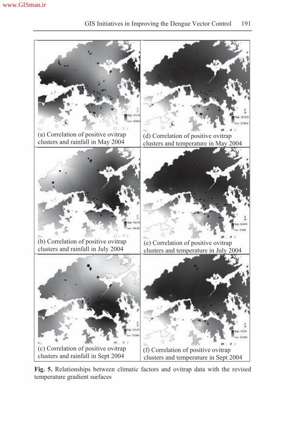
GIS Initiatives in Improving the Dengue Vector Control 191

(a) Correlation of positive ovitrap

clusters and rainfall in May 2004 (d) Correlation of positive ovitrap

clusters and temperature in May 2004

(b) Correlation of positive ovitrap

clusters and rainfall in July 2004 (e) Correlation of positive ovitrap

clusters and temperature in July 2004

(c) Correlation of positive ovitrap

clusters and rainfall in Sept 2004 (f) Correlation of positive ovitrap

clusters and temperature in Sept 2004

Fig. 5. Relationships between climatic factors and ovitrap data with the revised

temperature gradient surfaces

www.GISman.ir

192 Mandy Y.F. Tang and Cheong-wai Tsoi

Higher temperatures and excessive rainfall provide favorable conditions

for mosquito breeding. But the correlation between meteorological factors

and the mosquito population is not always straightforward and might be af-

fected by other underlying factors [6]. Public utilities like household water

supply and storage as well as solid waste disposal are also important envi-

ronmental determinants [1].

4 Discussions

This study has demonstrated that the GIS approach can be used to analyze

spatial patterns of vector borne diseases. Spatial analysis techniques in a

GIS can help determine the most likely areas of mosquito infestation. The

GIS techniques can also help understand correlations between climatic fac-

tors and vector surveillance data (e.g. ovitrap indices). The impact of cli-

matic factors such as temperature, rainfall and humidity on mosquito

breeding should not be belittle or oversimplified. A weak relationship be-

tween the mean temperature and dengue vector incidence was reported

from 1988 to 1992 in Puerto Rico [6]. Similar findings were found in the

Johor State of Malaysia [6]. Hence, analysis of a longer term is still neces-

sary to further confirm the effects of meteorological factors on the growth

of mosquito population.

Mosquitoes usually breed in pails, watering cans, discarded containers,

saucers of potted plants, and gully traps which contain stagnant water. In

fact, most of these “artificial” mosquito breeding sites may be made unin-

tentionally by people due to inadequate or improper waste management.

Some of these containers are of microscopic scale in GIS applications and

their dynamic nature makes them difficult to model in a GIS. Thus, in-

volvement of the community and public awareness on environmental hy-

giene are of paramount importance in the control of vectors for dengue fe-

ver .

5 Conclusions

This study illustrates that spatial statistical analysis can be applied to help

identify and visualize potential risk areas or hot spots affected by Aedes

albopictus. With the incorporation of surveillance data in a GIS, mosquito

activities can be tracked and monitored regularly and more efficiently. Ar-

eas repeatedly having positive ovitrap counts can be identified more read-

www.GISman.ir

GIS Initiatives in Improving the Dengue Vector Control 193

ily to target more focused cleaning activities. Furthermore, the study illus-

trates that rainfall and temperatures are two factors among others that af-

fect the breeding of mosquitoes. Without a doubt, a GIS is seen as a useful

tool that assist in decision making, adjusting monitoring scheme, deploy-

ing resources and coordinating cleaning efforts – all of which are essential

elements to controlling the spread of dengue fever in local communities.

But community involvement and awareness are also important in minimiz-

ing breeding grounds and the occurrences of mosquito infestation which,

in turn, contribute to the success of the dengue vector surveillance and

control programs.

Acknowledgements

The work described in this chapter was substantially supported by the de-

velopment team of the “HKSAR Geospatial Information Hub (GIH)” in

the Lands Department and ovitrap data from Risk Assessment and Com-

munication Division in the Food and Environmental Hygiene Department.

The authors thank both parties.

Reference

[1] Centre for Health Protection, Department of Health, HKSAR (2005) A Three-

Year Strategic Plan for the Prevention and Control of Dengue Fever in Hong

Kong Report of the Scientific Committee on Vector-borne Diseases

[2] CrimeStat Manual, Chapter 6 – ‘Hot Spot’ Analysis I

http://www.icpsr.umich.edu/CRIMESTAT/download.html

Accessed on April 5, 2006

[3] Food and Environmental Hygiene Department – Dengue Fever

http://www.fehd.gov.hk/safefood/dengue fever/index.html

Accessed on April 5, 2006

[4] Mitchell Andy (2005) The ESRI Guide to GIS Analysis vol 2: Spatial Meas-

urements & Statistics. Redlands, Calif: ESRI Press

[5] Schulz Travis, Bichler Mike, Voller Laura, Hoff Jennifer (2003) North Dakota

Mosquito Surveillance 2003 Program Division of Microbiology, Department

of Health, North Dakota

[6] Seng Su Bee, Chong Albert K, and Moore Antoni (2005) Geostatistical Mod-

eling, Analysis and Mapping of Epidemiology of Dengue Fever in Johor

State, Malaysia. Proceedings of the Seventeenth Annual Colloquium of the

Spatial Information Research Centre. 24 November to 25 November 2005,

Dunedin, New Zealand. University of Otago, pp 109-123

www.GISman.ir

194

[7] Tran Annelise (2001) Dengue Spatial and Temporal Patterns, French Guiana,

2001. http://www.findarticles.com/p/articles/mi m0GVK/is 4 10/ai n60764

45 Accessed on April 3, 2006

Remark

The authors work in the Land Information Centre of the Lands Department

in Hong Kong SAR, China. The views expressed in this chapter represent

the views of the authors and do not necessarily reflect the views of the

Lands Department or the Hong Kong SAR Government.

www.GISman.ir

Socio-Demographic Determinants of Malaria in

Highly Infected Rural Areas: Regional Influential

Assessment Using GIS

Devi. M. Prashanthia, C.R. Ranganathanb and S. Balasubramaniana

a Division of Remote Sensing and GIS, Department of Environmental Sci-

ences, Bharathiar University Post, Coimbatore, Tamil Nadu, India b Department of Mathematics, Tamil Nadu Agricultural University, Coim-

batore, Tamil Nadu, India

Abstract: Geographical Information Systems for disease surveillance play

a major role in public health and epidemiology. Malaria is a serious tropi-

cal disease and micro level mapping of the disease and its determinants are

necessary. Several studies have identified that the major malaria vector

Anopheles breeds in pools and streams and hence the people living in

close proximity to such breeding sites are at a high risk. The impact of to-

pography and human activities on the incidence of malaria was investi-

gated in a longitudinal trial study conducted in the highly endemic Vellar

region of Salem in India using a Global Positioning System (GPS) and a

Geographical Information System (GIS). A group of highly endemic vil-

lages and an uninfected village with similar topography were surveyed for

their geographical features, distance from house to breeding sites, the socio

economic living condition of a community (including the construction type

of houses), and the use of anti-malaria measures. The results indicated sig-

nificant relationships between the disease risk and the livelihood patterns

of the infected community like sanitation, livestock dependence, etc. A

comparative study against the uninfected village highlighted heterogene-

ous differences among the regions. Based on the integration of social, bio-

logical and geographical sciences, the present study provides the regional

malaria control authorities an opportunity to assess the risk of encounter-

ing the disease infection and to plan prevention measures accordingly.

Keywords: Malaria, disease surveillance, logistic regression

www.GISman.ir

196 Devi. M. Prashanthi, C.R. Ranganathan and S. Balasubramanian

1 Introduction

Natural ecosystems throughout the world have been severely altered by

human intervention (Tadei et al. 1998). The rapid urbanization in many

parts of the world is changing the context for human population and their

interaction with the natural ecosystem. To understand the complex nature

of the mosquito human relationship, it is required to identify the type of

human migration, population growth, socio economic status, behavior and

the environmental aspects around them. This requirement underscores the

importance of human intervention that may affect the mosquito vector

population and the intensity of parasitic transmission in endemic areas,

whether in rural or urban settings. The key determinants of the outcome of

malaria should be related to the human host, parasite, vector or environ-

mental parameters. However, the relative importance of these factors has

yet to be determined (Greenwood et al. 1991; Marsh 1992; Mbogo et al.

1999).

The habitats of the Anopheline vector and its ecological settings in rural

areas have been well documented by earlier studies (Minakawa et al. 1999;

Gimnig 2001; Chinery 1984; Barbazan 1998). Vector densities are nor-

mally higher in rural than urban areas due to favorable habitats (Coene,

1993). Poverty, farming activities, deteriorating infrastructure and over

crowding also contribute to the favorable conditions for developing mos-

quito breeding habitats (Keating et al. 2003). If households in a community

are unable to protect themselves, the risk of transmission of the disease in-

creases. Earlier studies have focused on identifying potential factors in ru-

ral areas that help the transmission of the disease such as the type of house

construction (Konradsen et al.2003; Hoek et al. 2003), socio economic

status of the public (Charlwood et al. 2003; Singh 2003), livestock de-

pendence (Mbogo et al. 1999), behavioral aspects among the residents

(Roper et al. 2000; Keating et al. 2003), drainage (Keating et al. 2003;

Eisele et al. 2003), distance to streams (Mbogo et al. 1999; Konradsen et

al. 2003; Hoek et al. 2003; Staedke et al.2003), and infectious-bite avoid-

ance pattern (Mbogo et al. 1999; Roper et al. 2000; Konradsen et al. 2003).

Understanding the influence of human activities on population dynam-

ics of the malaria vector is important in identifying areas in need of the

source reduction efforts and further control. To identify these factors, a

longitudinal study of malaria infected zones was carried out to record the

socio economic and the demographic data in highly endemic zones of the

Salem district using a questionnaire survey accompanied by a hand held

GPS (Garmin III Plus). As all the data were collected with household iden-

tifiers, opportunities for examining the spatial hypothesis exist. A map of

www.GISman.ir

Socio-Demographic Determinants of Malaria 197

the households and their related surveyed regions can be linked to existing

data sources through a GIS.

2 Study Area

Our study area is rather large and covers an size of 5494 sq. km. Surveying

an area of this size is a laborious task; therefore, we have selected a small

region within the study area for the epidemiological survey using a ques-

tionnaire and the Garmin III plus GPS (Figure 1). The study area chosen

for the survey was the Vellar PHC region based on its high infection rate

and the Santhaithanapatty PHC region as the controlled area. Three village

panchayats were surveyed which had seven hamlets in them. Thoppiar, a

major perennial stream, runs through these villages.

Fig. 1. Location of the study area

Only hamlets that could be visited either by walking or driving tractors

were chosen for the study. Each household was visited based on the house

number and the questionnaire was filled in by personal interview with the

residents. The living habitats of the people, occupational pattern and basic

village amenities were also enquired about. The distance from the hamlet

to the village hospital was also measured.

www.GISman.ir

198 Devi. M. Prashanthi, C.R. Ranganathan and S. Balasubramanian

3 Methodology

The survey was carried out during the month of October 2004 at four in-

fected villages that come under the Vellar PHC and one non-infected vil-

lage under the Santhaithanapatty PHC. The survey questionnaire included

queries of socio economic status, environmental conditions, human behav-

ior and possible locations of the breeding sites. Random sampling was

done in each village for a total of 206 samples which were geocoded using

the Garmin III plus GPS. The surveyed information was recorded into a

database and the input of data was facilitated with EpiInfo. The data were

later imported into the Arcview GIS 3.2a for further processing. The loca-

tions of the selected surveyed areas are presented in Figure 1. The Normal-

ized Differential Vegetation Index (NDVI) of these villages was calculated

using the ERDAS Imagine 8.5 image processing software for the subse-

quent month of Nov 2004 (Figure 2). The slope of the study area was also

computed from a Digital Elevation Model (DEM). The NDVI values, the

slope of each location and the obtained survey data were analyzed in SPSS

using Logistic Regression analysis for the determinants of the disease.

Fig. 2. Location of the surveyed area

www.GISman.ir

Socio-Demographic Determinants of Malaria 199

4 Statistical Analysis

Logistic Regression is an extension of the multiple linear regression

method and it is used when the dependant variable is dichotomous (non–

metric) and the independent variables normally are metric. Logistic Re-

gression is also known as Logistic analysis. This technique can be used to

describe the relationship of several predictor variables (X1, X2, …… Xk)

to a categorical dependant variable Y, typically coded as 1 or 0.

The expected value of Y (E(y)) is in the form of

k

j

jj X

yE

1

0exp1

1 Eqn (1)

The probability of the expected Logistic value i.e., the probability of

occurrence of any of the possible outcome y is rewritten as:

k

j

jj X1

0exp1

1Pr

Eqn (2)

The right head side of the equation 2 is the general expression of

sezf

1

1 Eqn (3)

where,

k

j

jjo Xz1

Eqn (4)

The function f(z) is called the logistic function and its values range

from 0 to 1 as z varies from - to + . This function is widely applied in

epidemiological modeling of the probability of a disease.

The general form of the logistic model is

Logit y = 0 + 1(X1) + 2(X2) + 3(X3) + 4(X4)+…+ K(YK) Eqn (5)

A conditional Multiple Logistic estimation was applied in the present

study for estimating the parameters (ß) to employ a conditional likelihood

function which led to the biased estimates of ß.

www.GISman.ir

200 Devi. M. Prashanthi, C.R. Ranganathan and S. Balasubramanian

Based on the above, a logistic model was proposed to postulate the

presence of mosquitoes (absence (0) / presence (1)). The equation (5) is

now rewritten for the present model as

Logit y = 0+ 1(X1)+ 2(X2)+ 3(X3)+ 4(X4)+ 5(X5)+

6(X6)+ 7(X7)+ 8(X8)+ 9(X9)+ 10(X10)+ 11(X11)

Eqn (6)

where,

Y = Presence of mosquitoes (No=0, Yes=1)

X1 = Vegetation (No=0, Yes=1)

X2 = Slope (No=0, Yes=1)

X3 = Drainage (No=0, Yes=1)

X4 = Wood storage (No=0, Yes=1)

X5 = Sanitation (No=0, Yes=1)

X6 = Livestock Dependence (No=0, Yes=1)

X7 = Waterbody (No=0, Yes=1)

X8 = Education (No=0, Yes=1)

X9 = House type (Reinforced concrete =0, Tiled=1, thatched =2,

Combined=3)

X10= Source of water (Tanks=0 Wells=1, Pipes=2, Open=3,

Closed=4)

X11= Prevention measure (No=0, Yes=1)

In multiple linear regression or any other regression models, the regres-

sion coefficients j play an important role in providing information about

the relationships of the predictors (independent variables) in the model to

the dependent variable. In a logistic regression, the quantification of these

relationships involves a parameter called “odds ratio’.

The odds ratio is expressed as

)Pr(

)Pr(

noevent

eventOdd = e 0 + 1X1 + KXK

Eqn (7)

The estimated odds ratio is the ratio of the probability of the occurrence

of some events divided by the probability that the same event will not oc-

cur. We used SPSS to compute the odds ratio of malaria incidences in the

surveyed areas using the aforementioned independent variables.

5 Results

Using the GPS values for the elevation of the surveyed households and

contour maps digitized through Arcview GIS 3.2a, a Digital Elevation

Model was generated to describe the slopes of the area (Figure 3). The ele-

www.GISman.ir

Socio-Demographic Determinants of Malaria 201

vation of the area varied from 250 m to 480 m above Mean Sea Level. The

slope values were derived from this map.

Fig. 3. Digital Elevation Model (DEM) of the surveyed study area

Slope is expressed as the change in elevation over a certain distance. In

this case, the certain distance is the size of the pixel. Slope is most often

expressed as a percentage but can also be calculated in degrees. The rela-

tionship between the percentage and degree expressions of a slope is as

follows:

• A 45º angle is considered a 100% slope

• A 90º angle is considered a 200% slope

• Slopes less than 45º fall within the 1 - 100% range

• Slopes between 45º and 90º are expressed as 100 - 200% slopes

For the present study slope was calculated in percentages and vary from

0% to 90%. This slope was attributed to the respective surveyed data to de-

termine the influence of slopes on mosquito breeding sites.

The NDVI, based on spectral reflectance properties, was calculated us-

ing the spectral analysis in ERDAS Imagine 8.5 (Figure 4). The NDVI is

used to identify the density of vegetation pattern of the selected areas and

it was used to recode the data into 3 vegetation classes: densely vegetated

area, scrublands or partial fields, and dry lands. These values were attrib-

uted to corresponding records in the database.

www.GISman.ir

202 Devi. M. Prashanthi, C.R. Ranganathan and S. Balasubramanian

Fig.4. Normalized Differential Vegetation Index (NDVI) of the surveyed study

area

A logistic approach was used to identity factors facilitating the proliferation

of mosquitoes in the surveyed areas based on the socio demographic data ob-

tained for the infected and controlled surveyed areas. The results are presented

in Table 1.

Table 1. The R square values for Model I and II for infected and uninfected areas

Pseudo R-Square Infected Areas

(Model I)

Controlled area

(Model II)

Cox and Snell 0.188 0.471

Nagelkerke 0.399 1.000

McFadden 0.326 1.000

Proximity to water bodies or thatched house type were two factors

found significant at the 5% level while reinforced concrete houses, tiled

houses and the avoidance behavior were significant at the 1% level. In

Model II for the controlled area, all the variables were found to be insig-

nificant for malaria proliferation (Table 2).

The fitted model II for the controlled area was

Logit y = 0 Eqn (9)

www.GISman.ir

Socio-Demographic Determinants of Malaria 203

Ta

ble

2

Lo

gis

tic

Reg

ress

ion a

nal

ysi

s of

the

surv

eyed

var

iab

les

of

infe

cted

are

a.

www.GISman.ir

204 Devi. M. Prashanthi, C.R. Ranganathan and S. Balasubramanian

6 Conclusion

From the results, it was inferred that among the 206 households surveyed,

the mosquito proliferation leading to malaria in the study area was found

dependent on the major driving factors identified in Model I. As the main

occupation of the people was farming, the economic status of the areas was

low and even below the poverty level. The people were found living close

to their farms and hence more likely infected due to proximity to stagnant

water in the fields and also still water caused by improper drainage that

provided breeding grounds for mosquitoes. The houses had mostly

thatched roofs. Even in cases of reinforced concrete housing, the adjacent

cattle barns were made of thatched roofs, which provided a suitable place

for the breeding of mosquitoes. The usage of open ground tanks for water

storage afforded another major breeding site. The lack of awareness of

proper sanitation facilities and avoidance behavior also added to the con-

text.

In addition, it was noted that people stayed outside their houses most of

the time i.e., they slept outside their houses in the evenings or at night

when mosquito activity was at its peak. These residents were mostly farm-

ers who wore partial or improper clothing to facilitate the daytime heat.

Mostly people reared cattles and other livestocks within their premises

which also led to constant and favorable conditions for mosquito prolifera-

tion. In the infected areas, the schools were situated closer to farms or had

water storage tanks nearby. This practice led to the children being infected

more than the adults.

Results of the present study identified target variables that potentially

favor mosquito breeding sites in the survey areas. The findings should help

in mobilizing social behavior and communication programs that may be

implemented to reduce the breeding sites based on community involve-

ment. Additionally, resource allocation can be recommended to infected

areas identified through population-based-surveys, which can be con-

ducted as a component of malaria control surveillance.

References

[1] Barbazan P, Baldet T, Darriet F, Escaffre H, Dhoda DH, Hougard JM, (1998)

Impact of treatments with B.sphaericus on Anopheles populations and the

transmission of malaria in Maroua, a large city in a savannah region of Cam-

eron. J.Am. Mos. Contrl Asso. 14:33-39.

[2] Charlwood JD, Pinto J, Ferrara PR, Sousa CA, Ferreira C, Gil V, Virgillo ER

(2003) Raised houses reduce mosquito bites, Malaria Journal 2:45

www.GISman.ir

Socio-Demographic Determinants of Malaria 205

[3] Chinery WA (1984) Effects of ecological changes on the malaria vectors

Anopheles funestes and the Anopheles gambiae complex of mosquitoes in

Accra, Ghana . J. Trop. Med. Hyg 87:75-81

[4] Coene J (1993) Malaria in Urban and rural Kinshasa: the entomological input.

Med Vet Entomol 7: 127-137

[5] Eisele TP, Keating J, Swalm C, Mbogo C, Githeko A, Regens JL, Githure JI,

Andrews L and Beier J C (2003) Linking field based ecological data with re-

motely sensed data using a geographic information system in two malaria en-

demic urban areas of Kenya. Malaria Journal 2:44

[6] Gimnig JE, Ombok M, Kamau L, Hawley WA (2001) Characteristics of larval

Anopheline (Diptera: Culicidae) habitat in western Kenya. J Med Entomol 38:

282-288

[7] Greenwood BM, Marsh K, Snow RW (1991) Why some African children de-

velop severe malaria? Parasitol Today 7: 277-281

[8] Hoek W, Konradson F, Amersinghe P H, Perara D, Piyaratne M K, Ameras-

inghe FP (2003) Towards a risk map of malaria in Srilanka: the importance of

house location relative to vector breeding sites. Int J Epidemiology 32: 280-

285

[9] Keating J, Macintyre K, Mbogo C, Githeko A, Regens JL, Swalm C, Ndenga

B, Steinberg L, Kibe L, Githure JI and Beier JC (2003) A geographical sam-

pling strategy for studying relationships between human activity and malaria

vectors in Urban Africa Am. J Trop. Med. Hyg 68(3): 357-365

[10] Konradsen F, Amerasinghe P, Hoek W, Amerasinghe F, Perara D, Piyaratne

M (2003) Strong Association between House characteristics and malaria vec-

tors in Srilanka Am. J Trop. Med. Hyg 68 (2): 177-181

[11] Marsh K (1992) Malaria- a neglected disease? Parasitol 104: S53-S69

[12] Mbogo CNM, Kabiru EW, Gregory EG, Forster D, Snow RW, Khamala

CBM, Ouma JH, Githure JI, Marsh, K and Beier JC (1999) Vector related

case control study of severe malaria in Kilifi district, Kenya Am. J Trop Med

Hygiene, 60(5): 781-785

[13] Minakawa N, Mutero CM, Githuire JI, Beier JC, Yan G (1999) Spatial distri-

bution and habitat characterization of anopheline mosquito larva in Western

Kenya. Am. J Trop. Med. Hyg 61: 1010-1016

[14] Roper MH, Torres RSC, Goicochea CG, Anderson EM, Guarda JSA,

Calampa, Hightower A W, Magill A J (2000) The Epidemiology of malaria in

epidemic area of the Peruvian Amazon Am. J Trop. Med. Hyg 62(2):247-256

[15] Singh N, Mishra AK, Shukla MM, Chand SK, (2003) Forest malaria in

Chhindwara, Madhya Pradesh, Central India: A Case study in Tribal Commu-

nity Am. J Trop. Med. Hyg 68(5): 602-607

[16] Staedke SG, Nottigham EW, Cox J, Kamya MR, Rosenthal PJ and Dorsey G

(2003) Short report: Proximity to Mosquito Breeding sites as a risk factor for

clinical malarial episodes in an urban Cohort of Ugandan Children. Am. J

Trop. Med. Hyg 69(3): 244-246

[17] Tadei WP, Tatcher BD, Santos JMM, Scarpassa VM, Rodrigues IB, Rafeal

MS (1998) Ecologic observations on Anopheline vectors of Malaria in the

Brazilian Amazon Am. J Trop Med Hyg, 59(2): 325-335

www.GISman.ir

A Study of Dengue Disease Data by GIS Software

in Urban Areas of Petaling Jaya Selatan

Mokhtar Azizi Mohd Din, Md. Ghazaly Shaaban, Taib Norlaila and

Leman Norariza

Department of Civil Engineering, Faculty of Engineering, University of

Malaya, 50603 Kuala Lumpur, Malaysia

Abstract: The MapInfo GIS software was used to map dengue data and

its relationship to the sanitary conditions in the study site of Petaling Jaya

Selatan, Selangor, Malaysia. The study utilized dengue data provided by

the Petaling Jaya Municipal Health Unit and it was integrated with the

Petaling Jaya map to pictorially present information about the affected

areas. The software gives a rapid identification of the locations of dengue

cases through a graphics display. This multi racial residential area reported

35 cases of dengue over a seven-month study commencing between

November 1998 and June 1999. The racial breakdown of patients was 57%

Chinese, 20% Indian and 23% Malay among which 54% was female and

46% male. Based on the on-site survey, it was observed that the affected

areas have very poor sanitary living conditions. This study concluded that

poor sanitary conditions were the most probable cause for the spread of

such a disease and the GIS technology has been proven efficient in data

collection and presentation of disease incidence for charting immediate

corrective and preventive actions.

Keywords: health, MapInfo Geographical Information System (GIS),

dengue, Aedes aegypti, improper drainage

1 Introduction

Dengue is transmitted by the Aedes aegypti mosquito species found pre-

dominantly in urban centers and in certain rural areas of Malaysia. It is

rarely observed at an elevation of 4,000 feet above sea level. This species

breeds in stagnant water and poorly drained areas.

www.GISman.ir

A Study of Dengue Disease Data in Petaling Jaya Selatan 207

Dengue fever is characterized by a sudden onset of high fever, severe

headaches, joint and muscle pain, nausea, vomiting and rash (National

Centre for Infectious Diseases 2000). The rash appears 3-4 days after the

onset of fever and the illness may last up to 10 days but complete recovery

can take 2 to 4 weeks. There is no known vaccine for dengue fever. Eradi-

cation is through preventative methods by instilling awareness on im-

proved public health through education and therefore improvement in gen-

eral hygiene is most crucial.

Previous work by Md. Ghazaly et al. (1998) on a similar research on

water quality and health investigated the impact of water quality and quan-

tity on human health. It was observed that a general improvement in both

the quality and quantity of water supplied to users was necessary to curtail

the spread of the disease. This was especially true for raw river water qual-

ity prior to treatment and post treatment at the water treatment plant. How-

ever, no direct link between raw water, treated water at the water treatment

plants and the disease could be ascertained due to inadequate information.

The importance of sanitation (including proper disposal of wastes) was

also emphasized in the prevention of the disease from spreading. At that

time, no GIS work was carried out due to the preliminary nature of the

work.

2. Role of GIS

The Mapinfo GIS software (MapInfo Corporation 1996) has the ability to

present dengue data spatially. Spatial data analysis involves describing

data related to a process operating in space, the exploration of patterns and

relationships in such data, and the search for explanations of such patterns

and relationships (Bailey and Gatrell 1995). Coupled with time based data,

useful information can be extracted from locational data and layering of

analytical outputs for visual presentation. Data about disease incidence, in-

cluding location and date of occurrence, can be incorporated easily in a

GIS for comprehensive analyses.

In this study, we managed to convert dengue data found in various

formats into the MapInfo GIS format. Having arranged the data in a

systematic way, the relevant authority was able to retrieve and view the

required information efficiently. This information on Dengue prevalence is

essential for town and urban planning units in coordinating and managing

works in environmental health.

www.GISman.ir

208 Mokhtar Azizi Mohd Din, et al.

3 Methodology

3.1 Selection of the study area

Petaling Jaya Selatan (PJS) was chosen because it is located in the urban

area where dengue cases are frequently reported in comparison to the other

areas of Petaling Jaya. Given the scope and time limitation of the study

and the availability of surveillance data, the investigation was focused on a

very limited area as indicated above (Norariza 2000). A digital map of the

study area in Petaling Jaya was obtained from the Jabatan Ukur dan Pe-

metaan Negara Malaysia (JUPEM).

3.2 Sources of Dengue Case Data

Dengue data was obtained from the Department of Health and Petaling

Jaya Municipal Council (Jabatan Kesihatan and Majlis Perbandaran

Petaling Jaya) or MPPJ. On-site surveys of the study area were also carried

out to identify possible factors to correlate with dengue, such as conditions

of sanitation, solid waste disposal and wastewater treatment system.

3.3 Data Input to MapInfo

The addresses of all reported dengue cases were input into the MapInfo

GIS. The location of each case was marked on a digital base map to see its

distribution within the study area. Other related information such as date,

age, gender, race, drainage system, solid waste disposal system, and build-

ing type were arranged as attributes to each case in a tabular format.

4 Analysis of Dengue cases

The study adopts a 5-step procedure for map digitizing and analysis.

Firstly, the digital map of Petaling Jaya in dxf format was imported to the

MapInfo GIS for further processing (Figure 1). Then, Dengue data was

aligned with the base map and mapped. The Dengue locations were linked

with the corresponding attributes for easy retrieval and display in MapInfo

(Figure 2). The map could be enlarged or zoomed in for a better view to

permit editing and analysis. Finally, the exact locations of the dengue cases

could be studied in relation to other factors.

www.GISman.ir

A Study of Dengue Disease Data in Petaling Jaya Selatan 209

Fig. 1. A digital base map of Petaling Jaya from JUPEM

Fig. 2. MapInfo showing attributes of selected cases

www.GISman.ir

210 Mokhtar Azizi Mohd Din, et al.

5 Results and Discussion

35 cases of dengue were reported over an eight month period from No-

vember 1998 to June 1999. The Dengue cases were reported monthly to

the hospitals and the patients for the study aged between 4 to 62 years old.

The breakdown of these cases by racial groups was 57% Chinese, 20% In-

dian, and 23% Malay, as indicated in Figure 3. There was an almost equal

split between the gender groups with 54% female and 46% male, as shown

in Figure 4.

Fig. 3. Dengue case according to race Fig. 4. Dengue case according to gender

Data obtained from the MPPJ indicated that each of the patients was

found to keep a container within their house, where the mosquitoes could

breed easily. Weekly on-site visits to the affected areas in September 1999

for one month yielded some interesting findings. Some of the areas exhib-

ited poor disposal of solid wastes. Most of the uncovered drains were

found to contain stagnant and foul water.

Primary findings in areas badly affected by Dengue included the follow-

ing observations: (i) abundance of man-made containers such as cans, bot-

tles, tires, flower pots, and others; (ii) inadequate solid waste disposal; and

(iii) inadequate drainage system. From the survey information, it was

found that the categories of waste disposal ratings (in 3 classes of bad, me-

dium, and good) had a strong influence on the number of cases of dengue,

as shown in Figure 5.

Fig.5. Solid waste disposal versus Dengue case

www.GISman.ir

A Study of Dengue Disease Data in Petaling Jaya Selatan 211

The Ministry of Health has taken reactive and proactive measures in

combating the dengue problems in Petaling Jaya Selatan and particularly

in places having a tendency for mosquito breeding. These measures in-

cluded the following:

educating the people about the importance of cleanliness and hy-

giene (Table 1)

periodic fogging of insecticide such as malathion (Table 2)

Table 1. Public awareness activities by MPPJ

SUBJECT YEAR

Health Awareness Education 1993 1994 1995 1996 1997

Health briefing 20 30 95 125 58

Video session 1 1 1 0 0

Demonstrations 0 0 0 0 0

Exhibitions 0 0 0 20 10

No. of posters and flyers 35,000 40,000 70,000 62,000 34,000

Table 2. Fogging activities by MPPJ (Aedes control / Fogging / Health education

activities)

Our study demonstrated that the application of MapInfo in examining

dengue data contributed to faster viewing and retrieval of critical health

and environmental information, as shown in Figure 6. Appropriate mitigat-

ing actions by the relevant authorities can be executed far more quickly

once the affected locations are identified.

Week No. of

Buildings

Checked

Building

With +Ve

Result

(Found

Aedes)

% OF

Building

(Found

Aedes)

Fogging

Activities

Cleaning

Activities

Health

Briefing

current

week4,066 57 1.4 10,697 0 0

last

week55,853 1,542 2.9 284,479 12 5

total 59,919 1,599 2.9 295,176 12 5

www.GISman.ir

212 Mokhtar Azizi Mohd Din, et al.

Fig. 6. MapInfo showing a full view of the area studied and patient databases

6 Conclusion

The use of MapInfo GIS in our investigation of the Dengue data yielded

some useful information about the disease. On-site visits to the area tended

to confirm the data obtained from the Ministry of Health. Factors such as

hygienic living conditions, proper disposal of solid wastes and effective

drainage play important roles in curtailing the spread of Dengue in the

long run. Short term measures of fogging may alleviate the problem to a

certain extent. Our future work will involve an exploration of statistical

analysis of health related data with environmental and locality factors.

Acknowledgements

The authors would like to thank the Department of Health of Petaling Jaya,

Petaling Jaya Municipal Council (MPPJ), Department of Surveying and

Mapping Malaysia (JUPEM) and staff of the Department of Civil Engi-

neering, University of Malaya for the technical information supplied and

their continuous support.

www.GISman.ir

A Study of Dengue Disease Data in Petaling Jaya Selatan 213

References

[1] Bailey TC and Gatrell AC (1995) Interactive spatial data analysis. 2nd edition,

Longman, Harlow

[2] MapInfo Corporation (1996) Map Info User Manual, version 4.5. Troy, New

York

[3] Md Ghazaly Shaaban, Zubaidah Ismail, Norjidah Anjang Abdul Hamid,

Sumiani Yusoff and Nik Meriam Sulaiman (1998) Impact of water quality and

quantity on human health. One day seminar on Recent Advances on Research

in the Water Industry. Malaysian Water Association, 28 July, Kuala Lumpur,

pp.1-17

[4] National Centre for Infectious Diseases (2000) Travellers Health. Virginia,

February

[5] Norariza Leman (2000) Application of GIS in dengue studies in Petaling Jaya.

B.Eng.(Environment) Thesis, University of Malaya, Kuala Lumpur

www.GISman.ir

A Spatial-Temporal Approach to Differentiate

Epidemic Risk Patterns

Tzai-hung Wena, Neal H Linb, Katherine Chun-min Linc, I-chun Fana,

Ming-daw Sud and Chwan-chuen Kingb

a Centre for Geographical Information Science, Research Centre for Hu-

manities and Social Sciences, Academia Sinica, Taipei, Taiwan b Institute of Epidemiology, College of Public Health, National Taiwan

University, Taipei, Taiwan c Department of Public Health, College of Public Health, National Taiwan

University, Taipei, Taiwan d Department of Bioenvironmental Systems Engineering, National Taiwan

University, Taipei, Taiwan

Abstract: The purpose of disease mapping is to find spatial clustering and

identify risk areas and potential epidemic initiators. Rather than relying on

plotting either the case number or incidence rate, this chapter proposes

three temporal risk indices: the probability of case occurrence (how often

did uneven cases occur), the duration of an epidemic (how long did cases

persist), and the intensity of a transmission (were the case of chronological

significance). By integrating the three indicators using the local indicator

of spatial autocorrelation (LISA) statistic, this chapter intends to develop a

novel approach for evaluating spatial-temporal relationships with different

risk patterns in the 2002 dengue epidemic, the worst outbreak in the past

sixty years. With this approach, not only are hypotheses generated through

the mapping processes in furthering investigation, but also procedures pro-

vided to identify spatial health risk levels with temporal characteristics.

Keywords: risk identification, spatial autocorrelation, spatial-temporal

analysis, epidemic

1 Introduction

In 1854, John Snow curbed the spread of cholera by identifying through

mapping the infected water pump located in the Golden Square of London

(Snow 1936). Ever since, mapping of infected cases has become an impor-

www.GISman.ir

A Spatial-Temporal Approach to Differentiate Epidemic Risk Patterns 215

tant means to generating hypotheses, guiding intervening measures, and

controlling infectious outbreak. Mapping can help epidemiologists to find

the origins of an outbreak, but more importantly, to target high-risk areas

and places of strategic importance in disease prevention (Ali et al. 2003).

A Geographical Information Systems (GIS) is often constructed under

these circumstances: a computer-based system is set up to integrate spatial

statistics into maps, which can detect disease clustering and determine re-

lationships between disease rates and relevant geographic locations (Lai et

al. 2004, Cockings et al. 2004, Dunn et al. 2001). Recent studies have

united temporal factors with spatial analysis and found dynamic epidemic

changes in certain time course and in specific locations (Tran et al. 2004,

Harrington et al. 2005, Morrison et al. 1998, João et al. 2004, Getis et al.

2003). Unlike the traditional approach, this chapter enhances spatial analy-

sis by using not only the incidence rate. We propose a spatial model that

integrates temporally-defined epidemiological characteristics and verify it

using data from the 2002 dengue epidemic in Taiwan.

Dengue virus, a member of flaviviruses with four known antigenic dis-

tinct serotypes, is transmitted in Taiwan mainly by mosquitoes of species

Aedes aegypti and Aedes albopictus. Few studies have focused on the in-

terplay between the spatial clustering of dengue cases and entomological

factors (Ali et al. 2003, Tran et al. 2004, Morrison et al. 1998) or environ-

mental conditions (Alpana and Haja 2001) by using a GIS with spatial sta-

tistics. However, spatial analysis is the key to identifying the incidence of

dengue fever (DF), dengue hemorrhagic fever (DHF) and dengue shock

syndrome (DSS). On the contrary, several studies have the treated tempo-

ral issues on dengue transmission (Tran et al. 2004, Harrington et al. 2005,

Morrison et al. 1998, Derek et al. 2004). Innovative models of temporal-

spatial analysis in disease transmission have proffered, and tested by data

of the 2002 dengue epidemic in Taiwan, which was the worst outbreak in

both magnitude and severity in the past sixty years. Hopefully this novel

approach of disease surveillance can be applied to detect other infectious

diseases.

2 Materials and Methods

2.1 Data of Dengue Confirmed Cases

Kaohsiung City and its satellite city of Fengshan, confronted in 2002 the

biggest dengue epidemic in Taiwan since 1940s. A total of 4,790 cases

were confirmed (representing 85% of total cases found in 2002), including

4,574 dengue fever (DF) cases and 286 dengue hemorrhagic fever (DHF)

www.GISman.ir

216 T.H. Wen, et al.

cases according to WHO’s definition (Chao et al. 2004). This study fo-

cuses on these 4,790 confirmed cases cohered with positive results in one

of the three following laboratory tests: (1) molecular diagnosis (Lanciotti

et al. 1992), or (2) serological diagnosis (Shu et al. 2001), or (3) virus iso-

lation (Kuno et al. 1985). Figure 1 illustrates the temporal progression of

DF versus DHF cases.

This chapter chooses Li - the smallest administrative unit in Taiwan - as

the spatial mapping unit, and a 7-day week as the temporal indicator. Most

Li in urban areas occupies 0.26-0.58 square kilometers and comprises

2,100-5,300 residents or 850-1,600 households. 423 Li covered roughly

94.4% of total confirmed dengue cases in 2002. These case data were pro-

vided by the Taiwan-CDC and without personal identifiers to protect the

privacy of the patients. All cases (including DHF cases) collected in this

chapter were summarized at the Li scale, instead of by exact addresses.

Fig. 1. The epidemic curve of week-based total confirmed dengue (DEN) and

dengue hemorrhagic fever (DHF) cases in Kaoshiung City and Fengshan City,

2002

2.2 Temporally-defined Indices as Epidemiological Measures

A risk model developed by Wen et al. (2006) depicts the dynamic process

of a dengue epidemic by emphasizing temporal characteristics on map dis-

plays. To evaluate a dengue epidemic in both magnitude and severity, this

chapter modifies and further introduces indices with temporally-defined

epidemiological characteristics (also referred to as temporal indices), in-

cluding (1) probability of occurrence or how often do cases occur in cer-

tain week(s) of a calendar year (e.g. 2002 in this study), (2) duration of

www.GISman.ir

A Spatial-Temporal Approach to Differentiate Epidemic Risk Patterns 217

epidemic or how long does an epidemic persist, and (3) intensity of

transmission or how significant do cases among people at risk happen

and cumulate in consecutive weeks during an epidemic wave. A higher

value of , , will indicate that a case studied is more likely to occur

within a specific time interval with a longer duration and more intense

transmission.

2.2.1 Probability of Occurrence Index ( )

, the probability of a disease occurrence in certain week(s), is the propor-

tion of one or more laboratory confirmed dengue cases occurred in an epi-

demic period (i.e.. numerator, EW) to the total number of weeks in that

year (i.e.. denominator, TW = 52). The mathematical definition of of a

specific disease is expressed in Equation 1 below:

TW

EW Eqn. 1

2.2.2 Duration of Epidemic Index ( )

To monitor the persistence of disease cases in a geographical area of inter-

est, the duration of an epidemic ( ) is described as the average number of

weeks per epidemic wave as in Equation 2:

EV

CWEV

i

i

1

Eqn. 2

where CWi represents the summation of persistent numbers of weeks for

the ith epidemic wave, and EV is the total number of epidemic waves in the

studying period. The duration index, reflecting the effectiveness of preven-

tive and control strategies used during the early period of an epidemic, is

very valuable for public health practitioners and administrators. A larger

value means fewer disease cases are eliminated.

2.2.3 Intensity of Transmission Index ( )

To measure population-adjusted mean magnitude of dengue cases per

wave, intensity of transmission equals to the mean number of case(s) oc-

curred in successive weeks divided by number of people at risk in an epi-

demic wave. Therefore, the intensity of transmission index ( ) is formu-

lated as in Equation.3:

www.GISman.ir

218 T.H. Wen, et al.

= (CaseNum/POP)/EV Eqn. 3

where CaseNum and POP represent respectively the cumulative total of

confirmed dengue cases and population-at-risk, and EV as described

above. The index is comparable to a measure of the intensity of cases in

different areas considering both the duration and size of the population. A

higher index implies that the occurrence of cases is temporally concen-

trated; whereas a lower value equates to a smaller epidemic wave, indicat-

ing that most cases are sporadic and temporally dispersed throughout the

epidemic. The use of different temporal indices offers clues to key ele-

ments of an epidemic that are worth investigating.

2.3 Spatial risk index: Local Indicator of Spatial Autocorrelation

Other than temporally-defined epidemiological characteristics, the degree

of spatial clustering among cases (i.e. spatial risk) (Odland 1988) is also

needed to measure the degree of association between an interested tempo-

ral index and its specified location. Spatial autocorrelation, including

global and local autocorrelation indices, are then introduced. A Positive

spatial autocorrelation and negative spatial autocorrelation in the Global

indices (Griffith 1987) respectively represent “clustering” of points based

on tested variables (Anselin 1995) and inverse correlation, shown as “spa-

tial outliers”, between neighboring areas. A zero spatial autocorrelation is

considered a random distribution rather than clustering or dispersal. Local

autocorrelation indices, however, evaluate trends of clustering by compar-

ing similarities and dissimilarities among neighboring locations. Therefore,

further information about clustered loci is gained. In brief, the Local Indi-

cator of Spatial Autocorrelation (LISA) can be regarded a spatial risk in-

dex to identify both significant spatial clusters and outliers (Anselin 1995).

The definition of LISA index is given below:

n

j

j

iji

XXW

XXiI

1

)()()(

Eqn. 4

where I(i) = the LISA index for region i; Wij = the proximity of region i to

region j; Xi = the value of the tested temporal index of region i; Xj = the

value of the tested temporal index of region j; X = the average value of

the tested temporal index; = the standard deviation of Xi; and n = the to-

tal number of regions to be evaluated.

www.GISman.ir

A Spatial-Temporal Approach to Differentiate Epidemic Risk Patterns 219

The term Wij describes the proximity between region i and j, where a

value of 1 means that region i is next to region j. The term

)()( XXXX jidescribes the degree of similarity in a tested index within

a designated area and its neighbors; from which each of temporal indices

for the 2002 dengue epidemic in Kaohsiung and Fengshan was evaluated.

A positive I(i) value of the tested LISA means that a certain region and its

neighboring areas exhibit a clustering of homogenous areas and have a

higher tendency of local spatial dependency. In contrast, a negative I(i)

value, which shows the opposite trend between Xi and Xj (i.e. Xi = high,

Xj = low or vice versa), implying a negative spatial dependency (i.e. the

region is a spatial outlier in relation to its neighborhoods). The Monte

Carlo significance test can be used to evaluate the statistical significance of

spatial clusters and outliers (Anselin 1995). Risk areas can be classified by

LISA index values into five distinct levels of epidemiological significance

(Table 1).

Fig. 2. Definitions of five spatial risk levels. Areas with a high value of the tested

index are shown in grey and areas with a low index value are shaded in white.

Among the five spatial risk distributions, (a) shows a spatial cluster of high values

of the tested temporal index; (b) and (c) represent the spatial outliers; (d) shows

random spatial distribution of the tested temporal index; and (e) displays a spatial

cluster of low values of the tested temporal index.

Risk Levels: (a) Extreme (b) High (c) Moderate (d) Mild (e) Lowest

Cell with high index value is shaded in grey Cell with low index value is shaded in white

www.GISman.ir

220 T.H. Wen, et al.

Table 1. Five spatial risk levels with epidemiological significance

Spatial

Risk Level Epidemiological Significance

Level 1

(Extremely

high)

Areas surrounded by neighboring areas having a statistically

significant positive LISA index and a high tested temporal index

value, shown in Figure 2(a), represent a spatial clustering of

such an designated temporal index. This implies the presence of

a severe epidemic spreading in that locality with extreme risk.

Level 2

(High)

Areas surrounded by neighboring areas with statistically signifi-

cant negative LISA index, where the central area has lower

tested temporal index value (as a spatial outlier) compared with

it’s neighbors, shown in Figure 2(b). This implies that a disease

outbreak would soon occur in these high-risk areas, if effective

control measures are not taken.

Level 3

(Moderate)

Areas surrounded by neighboring areas with statistically signifi-

cant negative LISA index, where the central area has higher

tested temporal index value (as a spatial outlier), opposite to

Level 2, compared with it’s neighbors, shown in Figure 2(c),

and implies that the focused area with moderate risk could be a

potential source of infection if cases begin appearing in the sur-

rounding areas.

Level 4

(Mild)

Areas surrounded by neighbors having neither a significantly

positive nor negative LISA index, shown in Figure 2(d). This re-

fers to cases occurred sporadically in those areas but there is no

significant spatial cluster or outlier.

Level 5

(Lowest)

Areas surrounded by neighbors having a statistically significant

positive LISA index, but low for the tested all the three temporal

index values, shown in Figure 2(e); this situation implies no

outbreak occurs in those areas.

3 Results

3.1 Correlation among three temporally-defined epidemiological Indices

All three temporal indices (including probability of case occurrence , du-

ration of epidemic , and intensity of transmission ) show significant

positive correlation with the “incidence rate” (p < 0.001) (Table 2). Among

the temporally-defined characteristics, intensity is strongly correlated with

duration ( and : 0.841), indicating that dengue cases in areas with a

higher intensity are most likely to persist (i.e. last a longer duration). Yet,

www.GISman.ir

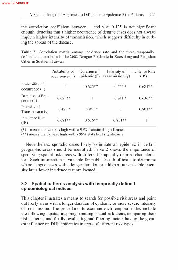
A Spatial-Temporal Approach to Differentiate Epidemic Risk Patterns 221

the correlation coefficient between and at 0.425 is not significant

enough, denoting that a higher occurrence of dengue cases does not always

imply a higher intensity of transmission, which suggests difficulty in curb-

ing the spread of the disease.

Table 2. Correlation matrix among incidence rate and the three temporally-

defined characteristics in the 2002 Dengue Epidemic in Kaoshiung and Fengshan

Cities in Southern Taiwan

Probability of

occurrence ( )

Duration of

Epidemic ( )

Intensity of

Transmission ( )

Incidence Rate

(IR)

Probability of

occurrence ( )1 0.625** 0.425 * 0.681**

Duration of Epi-

demic ( )0.625** 1 0.841 * 0.636**

Intensity of

Transmission ( )0.425 * 0.841 * 1 0.801**

Incidence Rate

(IR)0.681** 0.636** 0.801** 1

(*) means the value is high with a 95% statistical significance.

(**) means the value is high with a 99% statistical significance.

Nevertheless, sporadic cases likely to initiate an epidemic in certain

geographic areas should be identified. Table 2 shows the importance of

specifying spatial risk areas with different temporally-defined characteris-

tics. Such information is valuable for public health officials to determine

where dengue cases with a longer duration or a higher transmissible inten-

sity but a lower incidence rate are located.

3.2 Spatial patterns analysis with temporally-defined epidemiological indices

This chapter illustrates a means to search for possible risk areas and point

out likely areas with a longer duration of epidemic or more severe intensity

of transmission. The procedures to examine each temporal index include

the following: spatial mapping, spotting spatial risk areas, comparing their

risk patterns, and finally, evaluating and filtering factors having the great-

est influence on DHF epidemics in areas of different risk types.

www.GISman.ir

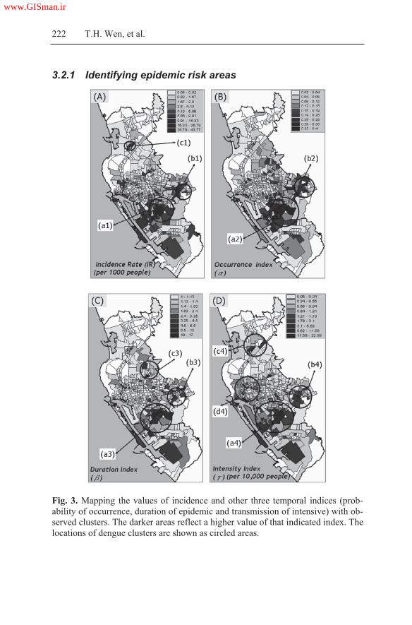
222 T.H. Wen, et al.

3.2.1 Identifying epidemic risk areas

Fig. 3. Mapping the values of incidence and other three temporal indices (prob-

ability of occurrence, duration of epidemic and transmission of intensive) with ob-

served clusters. The darker areas reflect a higher value of that indicated index. The

locations of dengue clusters are shown as circled areas.

www.GISman.ir

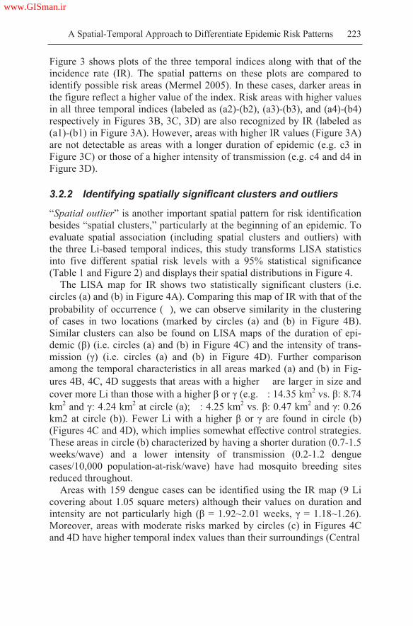
A Spatial-Temporal Approach to Differentiate Epidemic Risk Patterns 223

Figure 3 shows plots of the three temporal indices along with that of the

incidence rate (IR). The spatial patterns on these plots are compared to

identify possible risk areas (Mermel 2005). In these cases, darker areas in

the figure reflect a higher value of the index. Risk areas with higher values

in all three temporal indices (labeled as (a2)-(b2), (a3)-(b3), and (a4)-(b4)

respectively in Figures 3B, 3C, 3D) are also recognized by IR (labeled as

(a1)-(b1) in Figure 3A). However, areas with higher IR values (Figure 3A)

are not detectable as areas with a longer duration of epidemic (e.g. c3 in

Figure 3C) or those of a higher intensity of transmission (e.g. c4 and d4 in

Figure 3D).

3.2.2 Identifying spatially significant clusters and outliers

“Spatial outlier” is another important spatial pattern for risk identification

besides “spatial clusters,” particularly at the beginning of an epidemic. To

evaluate spatial association (including spatial clusters and outliers) with

the three Li-based temporal indices, this study transforms LISA statistics

into five different spatial risk levels with a 95% statistical significance

(Table 1 and Figure 2) and displays their spatial distributions in Figure 4.

The LISA map for IR shows two statistically significant clusters (i.e.

circles (a) and (b) in Figure 4A). Comparing this map of IR with that of the

probability of occurrence ( ), we can observe similarity in the clustering

of cases in two locations (marked by circles (a) and (b) in Figure 4B).

Similar clusters can also be found on LISA maps of the duration of epi-

demic ( ) (i.e. circles (a) and (b) in Figure 4C) and the intensity of trans-

mission ( ) (i.e. circles (a) and (b) in Figure 4D). Further comparison

among the temporal characteristics in all areas marked (a) and (b) in Fig-

ures 4B, 4C, 4D suggests that areas with a higher are larger in size and

cover more Li than those with a higher or (e.g. : 14.35 km2 vs. : 8.74

km2 and : 4.24 km2 at circle (a); : 4.25 km2 vs. : 0.47 km2 and : 0.26

km2 at circle (b)). Fewer Li with a higher or are found in circle (b)

(Figures 4C and 4D), which implies somewhat effective control strategies.

These areas in circle (b) characterized by having a shorter duration (0.7-1.5

weeks/wave) and a lower intensity of transmission (0.2-1.2 dengue

cases/10,000 population-at-risk/wave) have had mosquito breeding sites

reduced throughout.

Areas with 159 dengue cases can be identified using the IR map (9 Li

covering about 1.05 square meters) although their values on duration and

intensity are not particularly high ( = 1.92~2.01 weeks, = 1.18~1.26).

Moreover, areas with moderate risks marked by circles (c) in Figures 4C

and 4D have higher temporal index values than their surroundings (Central

www.GISman.ir

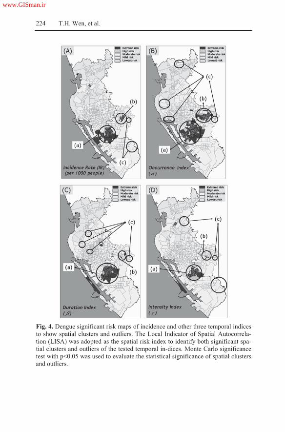
224 T.H. Wen, et al.

Fig. 4. Dengue significant risk maps of incidence and other three temporal indices

to show spatial clusters and outliers. The Local Indicator of Spatial Autocorrela-

tion (LISA) was adopted as the spatial risk index to identify both significant spa-

tial clusters and outliers of the tested temporal in-dices. Monte Carlo significance

test with p<0.05 was used to evaluate the statistical significance of spatial clusters

and outliers.

www.GISman.ir

A Spatial-Temporal Approach to Differentiate Epidemic Risk Patterns 225

vs. Surroundings: =1.5~3.1 vs. 0.03~0.6 weeks, =1.04~2.01 vs.

0.01~0.57). These areas might experience further outbreaks if mosquito

breeding sites were not eradicated. We can see that IR map alone (Figure

4A) without LISA map supplements (Figures 4B-4D) is not sufficient for

distinguishing spatial risk patterns among epidemiologically significant ar-

eas.

4 Discussion

This chapter proposes a minimum data requirement and more straightfor-

ward statistical methods to capture major temporal characteristics along

the dynamic epidemic process, and to suggest a workable procedure to in-

tervene in endemic or hyper-endemic developing countries of dengue (Ali

et al. 2003, Harrington et al. 2005, Morrison et al. 1998, Getis et al. 2003,

Derek et al. 2004). The integrated spatial-temporal characteristics, unlike

incidence rate alone, are useful in both nailing down risky areas and indi-

cating places that might have virus transmissible to facilitate and cause an-

other epidemic.

Temporal Epidemic patterns are complex. Although this chapter pro-

poses three temporally-defined epidemiological characteristics (probability

of occurrence, duration of epidemic, and intensity of transmission) to strat-

ify the severity of an epidemic, it is difficult to compare these indices with

each other in order of strength or severity measures. For example, which

one of temporal risk patterns exhibited by, for example, a high intensity of

transmission or a high duration of epidemic is more indicative? It is also

apparent from the discussions above that none of the indices is able to

stand alone. Clearly, further studies should focus on integrating three tem-

porally-defined epidemiological indices into ONE single risk index. Fur-

thermore, the effectiveness of this approach in identifying spatial-temporal

epidemic risk patterns should be evaluated in depth by considering multi-

year epidemic constructions, other diseases, and different locations.

In conclusion, the model proposed in this chapter can both quantita-

tively measure epidemiologically related temporal characteristics and

qualitatively evaluate the effectiveness of control measures based on

chronologically dynamic maps. Rather than relying on mapping cases or

incidence rate solo at different periods, this study enables public health ex-

perts additional options: (1) to comprehensively identify risk areas and ex-

amine their dynamic spatial-temporal changes throughout an epidemic, (2)

to provide broader perspectives with temporal risk characteristics other

than epidemic curves, and (3) to measure risk levels along with the sever-

www.GISman.ir

226 T.H. Wen, et al.

ity of epidemics after integrating spatial-temporal characteristics. Further-

more, monitoring spatial risk patterns over time described in this chapter

can as well be applied to other infectious diseases, such as the West Nile

encephalitis or Ebola hemorrhagic fever. Last but not least, the approach is

potentially useful for controlling the fast spreading and highly pathogenic

avian influenza virus (HPAI) by shortening the duration of the virus activ-

ity, and by minimizing its intensive transmission in epidemic sites; thus

avoiding a possible pandemic (Mermel 2005).

References

[1] Ali M, Wagatsuma Y, Emch M, Breiman RF (2003) Use of geographic in-

formation system for defining spatial risk for dengue transmission in Bangla-

desh: Role for Aedes Albopictus in an urban outbreak. Am J Trop Med Hyg

69(6): 634 – 640

[2] Alpana B and Haja A (2001) Application of GIS in Modeling of Dengue Risk

Based on Sociocultural Data: Case of Jalore, Rajasthan, India. Dengue Bulle-

tin 25:92-102

[3] Anselin L (1995) Local indicators of spatial association – LISA. Geogr Anal

27 (2): 93–115

[4] Chao DY, Lin TH, Hwang KP, Huang JH, Liu CC, King CC (2004) 1998

Dengue hemorrhagic fever epidemic in Taiwan. Emerg Infect Dis 10(3):552-4

[5] Cockings S, Dunn CE, Bhopal RS, Walker DR (2004) Users' perspectives on

epidemiological, GIS and point pattern approaches to analyzing environment

and health data. Health Place 10(2):169-82

[6] Derek C, Rafael I, Norden H, Timothy E, Ananda N, Kumnuan U, Donald B

(2004) Travelling waves in the occurrence of dengue hemorrhagic fever in

Thailand. Nature 427(22): 344-347

[7] Dunn CE, Kingham SP, Rowlingson B, Bhopal RS, Cockings S, Foy CJ, et al.

(2001) Analyzing spatially referenced public health data: a comparison of

three methodological approaches. Health Place 7:1 -12

[8] Getis A, Morrison AC, Gray K, Scott TW (2003) Characteristics of the spatial

pattern of the dengue vector, Aedes Aegypti, in Inquitos, Peru. Am J Trop

Med Hyg 69(5): 495 – 505

[9] Griffith DA (1987) Spatial Autocorrelation: A Primer. Resource Publications

in Geography (Washington: Association of American Geographers).

[10] Harrington LC, Scott TW, Lerdthusnee K, Coleman RC, Costero A, Clark

GC, et al. (2005) Dispersal of the dengue vector Aedes Aegypti within and

between rural communities. Am J Trop Med Hyg 72(2): 209 – 220

[11] Siqueira JB, Martelli CM, Maciel IJ, Oliveira RM, Ribeiro MG, Amorim FP,

Moreira BC, Cardoso DD, Souza WV, Andrade AL. (2004) Household Sur-

vey Of Dengue Infection In Central Brazil: Spatial Point Pattern Analysis

And Risk Factors Assessment, Am J Trop Med Hyg 71(5): 646–651

www.GISman.ir

A Spatial-Temporal Approach to Differentiate Epidemic Risk Patterns 227

[12] Kuno G, Gubler DJ, Velez M, Oliver A (1985) Comparative sensitivity of

three mosquito cell lines for isolation of dengue viruses. Bull World Health

Organ 63(2):279-86

[13] Lai PC, Wong CM, Hedley AJ, Lo SV, Leung PY, Kong J et al. (2004) Un-

derstanding the spatial clustering of severe acute respiratory syndrome

(SARS) in Hong Kong. Env Hlth Persp 112(15): 1560 – 6

[14] Lanciotti RS, Calisher CH, Gubler DJ, Chang GJ, Vorndam AV (1992) Rapid

detection and typing of dengue viruses from clinical samples by using reverse

transcriptase-polymerase chain reaction. J Clin Microbiol 30(3):545-51

[15] Mermel LA (2005) Pandemic avian influenza. Lancet Infect Dis 5(11):666-7

[16] Morrison AC, Getis A, Santiago M, Rigau-Perez J, Reiter P (1998) Explora-

tory space-time analysis of reported dengue cases during an outbreak in Flor-

ida, Puerto Rico, 1991-1992. Am J Trop Med Hyg 58: 287 – 298

[17] Odland J (1988) Spatial autocorrelation. Newbury Park, CA: Sage

[18] Shu PY, Chen LK, Chang SF, Yueh YY, Chow L, Chien LJ, et al. (2001) An-

tibody to the nonstructural protein NS1 of Japanese encephalitis virus: poten-

tial application of mAb-based indirect ELISA to differentiate infection from

vaccination. Vaccine 19(13-14):1753-63

[19] Snow J (1936) On the mode of communication of cholera. The Common-

wealth Fund. Oxford University Press, London

[20] Tran A, Deparis X, Dussart P, Morvan J, Rabarison P, Remy F, et al. (2004)

Dengue spatial and temporal patterns, French Guiana, 2001. Emerg Infect Dis

10(4): 615 – 621

www.GISman.ir

A “Spatiotemporal Analysis of Heroin Addiction”

System for Hong Kong

Phoebe Tak-ting Panga, Lee Phoebe a, Wai-yan Leung a, Shui-shan Leec,

and Hui Lina,b

a Department of Geography & Resource Management, Chinese University

of Hong Kong, Hong Kong, China b Institute of Space and Earth Information Science, Chinese University of

Hong Kong, Hong Kong, China c Centre of Emerging Infectious Disease, Chinese University of Hong

Kong, Hong Kong, China

Abstract: Heroin addiction is a socio-behavioral and medical condition

with significant public health implications. It is known that socioeconomic

factors and population changes are important forces shaping the pattern of

heroin addiction in a community. An understanding of these factors would

be useful for the planning of effective intervention strategies. We applied

the GIS technology in a study to display heroin addiction data over

consecutive years in 18 districts of the territory of Hong Kong. Correlation

was made between the proportions of heroin users in each district with the

following variables: (a) changes in the local population size and structure;

(b) economic attributes, in terms of employment and household income;

(c) social factors, notably education levels; and (d) access to drug

rehabilitation services, using methadone clinics as the surrogates. The data

were obtained from available repository including the Census data, service

statistics of methadone clinics, and Central Registry of Drug Abuse. The

spatiotemporal framework has enabled analyses from different

perspectives. We concluded that despite an overall decline in the number

of heroin users in Hong Kong over the years, proportional increases were

observed in selected districts. The association with poorer socioeconomic

indices was obvious and the coverage of methadone clinics was found to

vary from one district to another. The study offered a new means for

examining conventional data, which may be useful in fostering public

health policy development in the long run.

Keywords: GIS, heroin addiction, methadone clinics, spatial analysis

www.GISman.ir

230 T.T. Pang, et al.

1 Introduction

Heroin addiction has always been a major social problem in Hong Kong.

Although less than 1% of the total population was reportedly taking heroin

in the territory, a figure much lower than those of 4-5% in nearby South-

east Asian countries like Vietnam and Thailand (Department of Health,

2006), the potential threat of heroin addiction has continued to demand our

attention. In regard to prevention and control measures, it is necessary to

direct our attention to address socio-economic factors that may have trig-

gered the abuse of heroin. Besides eradicating heroin-related problems, it

would be beneficial to formulate measures to prevent people from heroin

addiction in the first place.

Heroin is considered a “hard” drug to distinguish it from other psycho-

tropic substances. The spatial distribution of heroin abusers is dictated

largely by their addictive behaviors and access to instant treatment. The

associated withdrawal symptoms when one is in need of heroin means that

one is not expected to travel too far to have the problem fixed. In this con-

nection, the Hong Kong government has established 20 methadone clinics

to provide treatment on demand. We assume therefore that heroin addicts

normally take heroin in their living regions and visit methadone clinics that

are within their living districts. Spatiotemporal analysis of heroin addiction

in Hong Kong would offer one means of describing the problem to inform

effective policies on prevention and control.

The Narcotics Division of the Security Bureau of HKSAR has been,

over the past 30 years, collecting drug abuse data through services like the

hospitals and Methadone clinics. The information is open to the public

through the Central Registry of Drug Abuse reports published twice a year.

Heroin addiction patterns are often described with charts and tables but

with little description of the geographic distribution. We piloted in this

study the development of a system to support spatiotemporal analysis of

heroin addiction in Hong Kong. The system involves not only the display

of heroin addiction data by districts, but also offers a platform to visualize

spatial pattern and temporal changes of heroin addiction, and to study the

relationships between heroin abusers and their socio-economic characteris-

tics. Data on methadone clinics are included in this system to allow users

an option to investigate their accessibility.

www.GISman.ir

A “Spatiotemporal Analysis of Heroin Addiction” System for Hong Kong 231

2 System Design And Development

A GIS is used as a tool in this project to draw spatial relationship between

the distribution of drug abusers and its correlation with districts and popu-

lation characteristics, as well as the coverage of existing methadone

clinics. The Spatiotemporal Analysis of Heroin Addiction system is de-

signed to offer a more comprehensive view on the issue of heroin addic-

tion in Hong Kong.

2.1 Data Source and Data Base Dictionary

A base map of Hong Kong was obtained from the Geography and Re-

source Management Department of the Chinese University of Hong Kong.

Data on heroin drug abusers came from the Central Registry of Drug

Abuse report. The population data for 2000 – 2004 were drawn from an

annual report entitled “Population and household statistics analyzed by

District Board district” published by the General Household Survey Sec-

tion of the Census and Statistics Department. Location of methadone

clinics and workload statistics were from the Department of Health and its

website (www.dh.gov.hk).

Fig.1. A data flow chart

www.GISman.ir

232 T.T. Pang, et al.

To sustain a comprehensive analytical system for users, different types

of data related to heroin addiction were prepared. These included data on

population demographics, methadone clinic locations, and district level

population statistics covering economic activities, income ranges, age

groups and education attainment (Figure 1).

2.2 System framework

As a database system and also an analytical tool, the Spatiotemporal

Analysis of Heroin Addiction system consists of two inter-related compo-

nents: the Heroin Addiction Spatial Analysis and the Methadone Clinic

Spatial Analysis. The existing database structure would support the organi-

zation of the datasets in a systematic way, making it easy for users to

search data and carry out appropriate analyses with the help of analytical

tools embedded in the System (Figure 2).

Fig. 2. A functional flow chart of the Heroin Addiction Spatial Analysis System

2.2.1 Heroin Addiction Spatial Analysis Subsystem

The Heroin Addiction Spatial Analysis subsystem is designed to support

the search for relevant data and to analyze heroin addiction patterns and

their relationships with population characteristics (i.e. income, education

attainment, economic status, and age group). This tool emphasizes on tem-

www.GISman.ir

A “Spatiotemporal Analysis of Heroin Addiction” System for Hong Kong 233

poral changes and specific statistical comparisons. To facilitate its use by

non-geographers wishing to focus on the statistics alone, the system is de-

signed to visualize spatial data in multiple representations. Heroin addic-

tion statistics can be displayed over time, or as charts and tables with ref-

erence to their spatial locations at the District level. Users can observe

heroin pattern changes over the years and the relationships with other

population variables at the same time. A special toolbox is designed for

creating graphs and buffers in support of further investigation.

2.2.2 Methadone Clinic Spatial Analysis Subsystem

The Methadone Clinic Spatial Analysis subsystem is an analytical tool for

assessing the geographic range of service and coverage of heroin addicts of

methadone clinics within a district. The system is designed on two as-

sumptions: All heroin addicts are evenly distributed within the districts and

the catchment area of methadone clinics appears circular in shape to yield

the highest coverage extending from the clinics. The “Range of service”

refers to the distance (or radius in this case) of the circular catchment area

from each clinic while “coverage” of the heroin population refers to the

proportion of heroin addicts that can be served within a district. Users can

perform the calculation by either inputting the range of service to yield the

coverage proportion or inputting the coverage proportion to get the maxi-

mum distance a clinic can serve.

Equation (1) is used to calculate the coverage of heroin addicts by input-

ting the range of service, while equation (2) is used to calculate the cover-

age of heroin addicts by inputting the coverage proportion.

Range of service2 * / Area of the district * Total number of

heroin addicts in that district * 100% Eqn. (1)

(Coverage proportion/ 100* Area of the district/ 3.14) ½

Eqn. (2)

The coverage of heroin addicts is further classified into different levels

for evaluating the efficiency of methadone clinics. This system is designed

for users who may wish to check the proportion of heroin addicts served

by clinics within a specific district at different assumption levels of walk-

ing distances.

www.GISman.ir

234 T.T. Pang, et al.

2.3 Software Requirement

The software required is the ArcMap GIS package, developed and mar-

keted by ESRI. ArcMap supports various kinds of spatial analyses, visuali-

zation of spatial data and execution of different modeling functions. The

Visual Basic Editor is also adopted for the programming of the system-

interface.

3 Applications

3.1 Documentation

The Spatiotemporal Analysis of Heroin Addiction 2006 system is equipped

with two powerful subsystems. Users may click on the Analysis button to

start either one of them. A Start dialog box with a welcome message will

pop up to prompt users into selecting either the ‘Hong Kong’ option (rep-

resenting the Heroin Addiction Spatial Analysis subsystem) or the ‘Metha-

done Clinic’ option (representing the Methadone Clinic Spatial Analysis

subsystem). The ‘What is this?’ button next to the options offers an expla-

nation of these choices (Figure 3).

Fig. 3. The start dialogue box and the explanation message box

3.2 Applications of Heroin Addiction Spatial Analysis

The Heroin Addiction Spatial Analysis subsystem has two drop down lists.

The first provides 6 categories of socio-economic factors related to heroin

addiction, namely ‘Number of heroin abusers’, ‘Number of population in

each district’, ‘Education attainment’, ‘Income range’, ‘Economic activity’

and ‘Income group’ (Figure 4). The second drop down list allows the

choice of an attribute from the chosen category of data, and then the time

www.GISman.ir

A “Spatiotemporal Analysis of Heroin Addiction” System for Hong Kong 235

bar will be activated. The legend of for the map display is shown at the

bottom left portion of the dialog box.

Fig. 4. The dialogue tool box of Heroin Addiction Spatial Analysis

In terms of map displays, users may visualize the chosen socio-

economic data of a particular year represented as a choropleth map (Figure

5) and its progressive changes over time by dragging the time bar. The

magnitudes of data in a choropleth map are represented in different shades,

with darker tones indicating larger values.

Fig. 5. A map showing variation of area-based data in different shades

www.GISman.ir

236 T.T. Pang, et al.

Graphs/charts of the chosen data can be produced in place of area shad-

ings by simply clicking on the Graph button which enables users to com-

pare the observed results on both maps and graphs at the same time. To be

more user-friendly, a Graph Wizard and a message box will pop-up when

users click on the Create Graph button. The making of graphs is stepped

through a few online instructions. It is noteworthy that the graphs pro-

duced will be automatically saved by the Graph manager for easy retrieval

at a later date.

3.3 Applications of Methadone Clinic Spatial Analysis

The Methadone Clinic Spatial Analysis subsystem allow users to obtain

basic information about a particular clinic from the Table of Content or all

clinics by activating the layer number 20 to show them concurrently. The

activated clinic layers will have the location of each clinics marked by a

glass filled with a green-colored methadone. Details of a particular clinic

such as the number of effective registration of methadone patients for each

month in 2004 and particulars of that methadone clinic will be shown in a

small window (Figure 6) by first clicking the Identify button on the tool

bar and then placing the mouse cursor over the clinic on the map.

Fig. 6. Identify results of a clinic on the map

www.GISman.ir

A “Spatiotemporal Analysis of Heroin Addiction” System for Hong Kong 237

Fig. 7. Dialogue tool boxes for Methadone Clinic Spatial Analysis

With the Methadone Clinic Spatial Analysis subsystem, users can

choose one methadone clinic from the drop down list in the Start dialogue

box. Then, the district name of the selected clinic will appear at the bottom

of the drop list. Users can key in the time equivalent in minutes of the

walking speed of heroin addicts for a distance of one kilometer. The total

required walking time to the range of services will be shown below the

“Load” button (Figure 7).

There are two methods to assess the efficiency of clinics, which is either

by determining the Range of Service (Figure 7a), or by determining the

Coverage of heroin population (Figure 7b). For example, users can deter-

mine the proportion of coverage by adjusting the radius of the sphere of

access for each clinic, or find out the maximum distance a clinic can serve

for a certain proportion of the coverage. The input data and calculated re-

sults are shown in the space at the bottom half of the dialogue box. The

level of efficiency is computed as the proportion of coverage in which a

higher figure implies a clinic with greater efficiency where more heroin

addicts in the population are served.

Users may proceed with another analysis on a different clinic by press-

ing the Reset button to make a new selection from the drop down list, fol-

lowed by a new walking distance, range of service, or the cover propor-

tion. The spatial coverage of each clinic can be displayed on a map having

completed the calculation. The Create Buffer button can be used to invoke

the buffer wizard to prompt users for values to draw buffers on a map.

(a) (b)

www.GISman.ir

238 T.T. Pang, et al.

3.4 Start Over

Users may return to the Start dialog box and press Quit to exit the system.

Another dialog box will pop up for confirmation of quitting the system in

which users should select “Yes” to end the session. Users are now back at

the interface where the project began.

4 Discussion

The system offers some interesting observations. On the overall situation

of heroin addiction in Hong Kong, the top 3 districts with the highest abso-

lute number of heroin abusers for 2002-2004 were Sham Shui Po, Yau

Tsim Mong and Kwun Tong, while Sai Kung, Central and Western Island

were the 3 lowest. Expressed in number per 10,000 population, the highest

were Yau Tsim Mong and Sham Shui Po and the lowest being Shatin and

Sai Kung. There was a difference between the two comparisons due to

variation in the district population. Sham Shui Po and Yau Tsim Mong

were smaller districts with a low population and therefore registered a rela-

tively large number of heroin abusers per 10,000 population. Kwun Tong

on the contrary had a large absolute number of heroin abusers but the pro-

portion was relatively small. In Shatin, the absolute number of heroin

abusers was in fact not very high, but it was characterized by a high preva-

lence because of the small denominator.

Population structure was a determining factor in another observation.

We found that the absolute number of heroin abusers in all districts de-

creased significantly but the decrease in the number of abusers per 10000

people was very small. For example, the number of heroin addicts in Tuen

Mun decreased from 900 to 810 between 2002 and 2004, but the preva-

lence per 10,000 population remained the same. Despite an overall decline

in the number heroin users in Hong Kong over the years, proportional in-

creases were observed in selected districts, such as the Islands. It seems

that the real situation of heroin addiction in Hong Kong has remained the

same rather than improved.

A comparison of the population characteristics produces interesting re-

sults. Sham Shui Po and Sai Kung with approximately the same population

size had the former registering the 2nd highest prevalence of heroin addicts

while the latter showing the lowest number. Compared with Sham Shui Po,

Sai Kung had a larger number of households of the high income groups,

more people with a higher education, and a lower proportion of the elderly

population. The number economically inactive population was also lower

in Sai Kung. It can thus be inferred that population characteristics differ

www.GISman.ir

A “Spatiotemporal Analysis of Heroin Addiction” System for Hong Kong 239

between districts irrespective of a higher or lower prevalence of heroin

abusers expressed as a proportion of the population. Areas with a higher

proportion of high income group, educated people, younger population and

more economically active population tend to be associated with fewer her-

oin abusers.

Table 1. Coverage proportion of different clinics

Name of clinic Level of coverage District located

Aberdeen 3 Central and Western

Eastern Street 1 Southern

Shau Kei Wan 2 Eastern

Violet Peel 3 Wan Chai

Ho Man Tin 4 Yau Tsim Mong

Hung Hom 3 Kowloon City

Kwun Tong 3 Kwun Tong

Li Kee 3 Kowloon City

Ngan Tau Kok 4 Wong Tai Sin

Robert Black 4 Wong Tai Sin

Sham Shui Po 4 Sham Shui Po

Wu York Yu 4 Wong Tai Sin

Yau Ma Tei 4 Yau Tsim Mong

Cheung Chau 1 Island

Lady Trench 1 Tsuen Wan

Sha Tin 1 Sha Tin

Shek Wu Hui 1 North

Tai Po 1 Tai Po

Tuen Mun 1 Tuen Mun

Yuen Long 1 Yuen Long

* Level 1: 0 25%; Level 2: 26 50%; Level 3: 51 75%; Level 4: over 75%

Source: Department of Health, 2006

The Methadone Clinic Spatial Analysis yields other interesting findings.

We set a walking speed at 15 min/km and obtained a range of service of

1.5 km. We then made an assumption that an average person or a heroin

addict was prepared to walk 22.5 minutes to access a service. Table 1

shows that with the range of service kept constant, clinics located in Kow-

loon had the highest average coverage proportion and level of coverage.

The level of coverage of clinics in Hong Kong Island was lower while that

in the New Territories was the lowest. Apparently districts in Kowloon are

smaller in size and therefore the clinics can serve a larger proportion of the

districts and hence more heroin addicts.

www.GISman.ir

240 T.T. Pang, et al.

Obviously, with the same range of service, it would be difficult for clin-

ics in the districts of New Territories to cover a large proportion of areas. It

is also understandable that the New Territories have fewer clinics as the

absolute number of heroin abusers is generally smaller, thus less demand

for the service. In some districts like Yuen Long, which has a relatively

higher number of heroin abusers than other parts of the New Territories,

there may not be sufficient methadone services to meet the need. From the

above analysis, we may conclude that there is a need to review the geo-

graphic distribution of Methadone clinics to suit the latest trends and needs

of heroin abusers.

5 Advantages and Limitations

This system is a pilot project built on the spatial method to support analy-

sis of heroin addiction problems. There is the advantage of effective utili-

zation of available data. Both heroin addiction data and population data are

integrated in one system such that the inter-relationships can be observed

and investigated. Numerical numbers and tables are transformed into spa-

tial data or maps to illustrate concurrently their variations across districts

and the patterns of distribution. Users can have a board overview of heroin

addiction in Hong Kong. Another advantage is that the system supports a

variety of functions like graphing and buffering to enable users to perform

multiple analyses at the same time.

A major limitation of the system is however the small amount of data

available given time limit and administrative problems. Data on population

characteristics are insufficient to support a more extensive analysis, includ-

ing the predisposing factors of heroin addiction. For example, it would be

desirable to include in the analysis such fields like gender and housing

type of population. However, it is difficult with limited heroin addiction

data to see the long term temporal change of heroin abuse and perform fu-

ture projection. While a considerable amount of data have been collected

under the Central Registry of Drug Abuse, there are restrictions in acquir-

ing data not currently included in the regular publications.

Another limitation is about the user interface. As a searching and an

analytical tool, the Analysis system is generally useful to users. But given

technical imperfections, users must exit the system to create graphs and

buffers and they cannot use toolbar functions like zoom in and zoom out

when the Analysis System is on. It would be more convenient if the

Analysis System and the toolbar functions can be both functional at the

same time. Other limitations include a slower loading speed for the graph-

www.GISman.ir

A “Spatiotemporal Analysis of Heroin Addiction” System for Hong Kong 241

ics version without which users may not know exactly which layers should

be chosen in the Graph Wizard to create the graphs they have in mind.

Despite the technical limitations, the system is unquestionably a valu-

able tool to transform numerical data into spatial data, along with support

for the application of spatial analysis on a socio-medical issue.

6 Potentials and Future Development

The Spatiotemporal Analysis System of Heroin Addiction system is only

the beginning of a new platform for gathering heroin abuse data in a GIS

system and presenting it in a more organized way. The pilot system has

compiled only 5 years worth of data. The next step would be an extension

of the system to gather and organize data of earlier periods from 1976 to

the latest available data.

The trend of drug addiction is changing. Heroin addition is usually found

among people of older ages. There are many new substances of abuse such

as Ketamine, Triazolam, MDMA (Ecstasy), Cannabis and

Methylamphetamine (Ice), the distributive patterns of which have also

been changing. With the collation of data collected by the Central Registry

of Drug Abuse, not only would heroin addiction data be researched, but

that data of other substances of abuse be input into the system to form a

central information system, so that the trends can be analyzed effectively.

Currently, GIS-based systems are not widely available in the territory of

Hong Kong. In the long run, the system should be developed into a web-

based service for easy accessibility by people who need it. The system

should consist of both ordinary (like the number of drug abusers in each

district, or the address and number of heroin abusers served by each

Methadone clinic in tabular formats) and complicated or statistical data

(such as correlations between age and type of drugs abused). A web-based

system would be an ideal solution for a simple and user-friendly imple-

mentation. Sharing of drug addiction data not only can increase the value

of the data but also the feedback and opinion of users from different sec-

tors of the society can improve the system by bringing in new and different

points of view on the issue.

This analysis of heroin addiction can in the future help public health of-

ficials open up another dimension for research, that is the geospatial corre-

lation of diseases transmitted among drug abusers. Knowing that needle-

sharing among heroin abusers is one of the ways of transmitting blood-

borne infections, knowledge on the pattern of heroin abuse can naturally

help track the transmission of infections.

www.GISman.ir

242 T.T. Pang, et al.

Acknowledgements

We thank the Department of Health for the provision of data on methadone

clinics, the Narcotic Division for data from the Central Registry of Drug

Abuse, and the Hong Kong Census and Statistics Department for the popu-

lation data.

References

[1] Department of Health (2006) Department of Health. Retrieved on 28 March

2006 at http://www.info.gov.hk/dh/index.htm

[2] Household Survey Section (1) (2000) Population and household statistics

analyzed by District Board district. Hong Kong: Census and Statistics De-

partment

[3] Household Survey Section (1) (2001) Population and household statistics

analyzed by District Board district. Hong Kong: Census and Statistics De-

partment

[4] Household Survey Section (1) (2002) Population and household statistics

analyzed by District Board district. Hong Kong: Census and Statistics De-

partment

[5] Household Survey Section (1) (2003) Population and household statistics

analyzed by District Board district. Hong Kong: Census and Statistics De-

partment

[6] Household Survey Section (1) (2004) Population and household statistics

analyzed by District Board district. Hong Kong: Census and Statistics De-

partment

[7] Narcotics Division of Security Bureau (2004) Central Registry of Drug Abuse

reports 54th Report 1995 – 2004, Narcotics Division of Security Bureau

www.GISman.ir

A Public Health Care Information System Using

GIS and GPS: A Case Study of Shiggaon

Ashok Hanjagia, Priya Sriharib, and A.S. Rayamanec

a Associate Professor, Department of Geography & Geoinformatics, Ban-

galore University, Bangalore- 56 India b Guest Faculty, Department of Geography & Geoinformatics, Bangalore

University, Bangalore-56 India c Professor, Department of Geography & Geoinformatics, Bangalore Uni-

versity, Bangalore-56 India

Abstract: Health data maps and Geographic Information Systems (GIS)

are significant resources for health planning and health services delivery,

particularly at the local level. The ability to visualize the spatial

distribution of health status determinants and indicators can be a powerful

resource for mobilizing community action to improve the health of

residents. Currently, health data maps and other GIS applications tend to

be highly technical and specialized, and are therefore of limited use to

community members and organizations providing community-based health

services. Developing relevant, accessible, and usable GIS and health data

maps for communities and local agencies is an important step towards

enabling individuals and communities to improve their health and increase

their control over it. The final map was prepared by overlaying all the

layers generated. The spatial objects were digitized out of LISS and PAN

merged data and topomap supplied by the NRSA and Survey of India

respectively. Questionnaires were prepared to get the data needed from

each hospital and house by field investigation. Finally, a map of Public

Health Care Information System was created by interlinking all

topographical features with attribute data of the town so as to keep this

information for planning and development in days to come.

Keyword: public health care system, GIS, GPS

1 Introduction

Health and life expectancy generally improve as societies develop but the

major causes of illnesses and deaths will also change. The mapping of

www.GISman.ir

244 Ashok Hanjagi, Priya Srihari and A.S. Rayamane

towns and cities (showing health centers, pharmacies, health camps, etc.)

and creation of databases using recent technologies have become more sig-

nificant both as an academic discipline and as one of the foundations for

practical decision-making (e.g. in governmental, administrative and other

public health care organizations) towards finding solutions of health re-

lated problems. It is generally known that the general public does not know

where hospitals are located, what facilities and the kinds of specialists are

available? Such problems can be addressed effectively by mapping and

creating relevant databases using a GIS.

The call for streamlining of health care operations as a means of achiev-

ing greater cost-efficiency is a positive sign in the development of a soci-

ety. Community leaders searching for innovative methods for health care

management have begun to recognize the power of a GIS in various man-

agement activities ranging from determining intervention strategies to

formulating health care reforms. Through the geo-coding process, a GIS

allows personal health data to be examined spatially so that patterns can be

discerned. Furthermore, geo-referencing of personal health data can

greatly enhance decisions made by public health officials. The tremendous

potential of a GIS to benefit the health care industry is just now beginning

to be realized. Both public and private sectors (including public health de-

partment, public health policy and research organizations, hospitals, medi-

cal centers, and health insurance organizations) are beginning to harness

the data integration and spatial visualization power of a GIS.

A GIS plays a critical role in the decisions on where and when to inter-

vene, improving the quality of care and accessibility of services, finding

the most cost effective delivery modes, and protecting patient confidential-

ity while satisfying needs of the research community on data accessibility.

The GIS technology has been used in public health care for epidemiologic

studies, as in tracking the sources of diseases and its spread in the commu-

nities such that authorities can respond more effectively to outbreaks of

diseases with appropriate intervention measures to the at-risk population.

GIS Applications in public health include tracking of child immunizations,

conducting health policy research, and establishing health service areas

and districts. A GIS not only provides a way to move data from the project

level to become a ubiquitous resource for an entire organization but also

renders the visualization of clinical and administrative data as a spatial de-

cision support tool.

As towns have grown larger as a result of urbanization and industrializa-

tion, the concentration of population has in turn led to complicated health

issues. A proper understanding of the roots of health problems is essential.

In this connection, an understanding of the spatial occurrences of various

diseases in urban area is a must for rational planning and management.

www.GISman.ir

A Public Health Care Information System Using GIS and GPS 245

Knowledge about characteristics of the population and the diseases can be

derived from GIS and Remote Sensing technologies.

Many health-related problems and determinants in the North Karnataka

state of southern India have been discussed in research papers. These pa-

pers also shed light on causes, differential incidence and socio-spatial con-

sequences of ill health within the towns. The town of Shiggaon, a taluk

headquarter, was selected for this research. Shiggaon is situated between

latitudes 14o59'24''N and 15o00'02"N and longitudes 75o12'36"E and 75o13'48"E (Figure 1). The total study area measures 20.74 sq. km. with an

annual precipitation of about 350 cm. Precipitation occurs in two seasons,

mainly between June and September as well as between October and No-

vember. The mean annual temperature ranges from 22.8oC to 27.8oC. The

population of Shiggaon consists of Hindu (70%), Muslim (29%), and oth-

ers (1%). Socio-economic, demographic, and standard of living data of

Shiggaon’s population were gathered by questionnaire surveys. Projections

on human needs were also made.

Fig. 1. A location map of Shiggaon town

The research aims at mapping Shiggaon to show the distribution of hos-

pitals, clinics, and dispensaries, in addition to assembling a database on

them. The public health care system concerns not only the health, well-

being, and functioning of the population but also offers the ability to visu-

alize spatial distribution (e.g., ward-wise) of health status indicators and

other health-related information (Figure 2). Both GPS and ArcGIS soft-

www.GISman.ir

246 Ashok Hanjagi, Priya Srihari and A.S. Rayamane

ware were used to demarcate the town’s boundaries, locate hospitals and

delimit disease vulnerable zones (Figure 3). Here, a GIS was used to col-

lect, integrate and display population-based data concerning health events

(including disease exposures, risk factors and socio-economic data).

Fig. 2. Distribution of hospitals and medical shops

Developing a GIS with the relevant health data that are accessible and

useable by the communities and local agencies are important steps toward

realizing the goal of enabling individuals and communities a better control

over their personal health. A GIS provides a supportive environment for

population-based public health program planning, program evaluation, and

community based decision-making. In the end, health-related information

will be available for the public of Shiggaon located in the western parts of

middle Karnataka (India) in the Haveri district.

www.GISman.ir

A Public Health Care Information System Using GIS and GPS 247

Fig. 3. Medical facilities and disease zones

2 Major Diseases in Shiggaon

2.1 Heart Related Diseases

WHO and various health organizations declared 2006 as the year of pre-

vention. A major disease for prevention in Shiggaon is the cardiac disease

and sudden cardiac death as these diseases have been spreading rapidly

and reaching epidemic proportions. A 2005 survey of the 25-60 age-groups

of Shiggaon revealed that half of the total death was from heart attack and

heart-related problems. An even more startling fact is that one fourth of

those with heart problems never reached hospitals to receive definitive

treatment. If this was the fate of the population of a medium sized town,

imagine the plight of people in the traffic chaos of Delhi, Mumbai,

Kolkota, Chennai, Bangalore, and Hyderabad. Cardiologists have indicated

that individuals with prior records of a heart attack have a higher risk of

subsequent attacks. Given that the conditions of a heart attack patient can

www.GISman.ir

248 Ashok Hanjagi, Priya Srihari and A.S. Rayamane

deteriorate very fast, adequate facilities must be made available to meet

this kind of emergency. Angioplasty services should also be made avail-

able in each town to rid the need of patients going to major cities for

treatment, which incurs much time and cost.

Preventive steps to avoid a heart attack, such as blood tests to detect the

disease risk, are essential services. In addition, CT Angiography, a simple

and noninvasive procedure to test the blockage in blood vessels, should be

made available to individuals at risk. These individuals would include men

over the age of 40, women over the age of 50, patients with diabetes melli-

tus and/or hypertension, obese individuals, smokers, and those with a fam-

ily history of heart attacks. Such CT Angiography facilities are now only

available in larger cities and not in towns.

2.2 Diabetes Mellitus

A recent survey conducted in Shiggaon indicated that 4 per cent of the

town’s population has Diabetes Mellitus, of which around 20 per cent are

adults. The major causes of this disease are bare foot walking and the rapid

onset and spread of infection once the foot sustains an injury. Foot prob-

lems have remained one of the most serious and expensive complications

of Diabetes Mellitus and the divesting effects are already felt in Shiggaon.

While advances in health care can help in early detection of the disease,

educating the public on preventive measures are a must. For example, one

should not walk barefoot indoor as well as outdoor and use correct foot-

wear as prescribed by physicians. A daily inspection of the feet for blisters,

wounds, bleeding, smell, or increased temperature is also recommended.

2.3 HIV/AIDS

Acquired Immune Deficiency Syndrome (AIDS) was first recognized in

1981. A large proportion of adults and children are infected daily. Because

of high fatality and the lack of effective treatment or vaccine, the

HIV/AIDS has emerged as one of the most serious health problems in In-

dia. In terms of income and wealth, AIDS has been found to associate with

poverty and ignorance in Shiggaon. The percentage of HIV infected people

living in the town should be higher than that reported officially as many

are not aware that they are infected according to statements made by phy-

sicians. There were reportedly 55 confirmed AIDS cases in 2005 and about

20 percent HIV infected individuals in Shiggaon, according to sources

from local hospitals.

www.GISman.ir

A Public Health Care Information System Using GIS and GPS 249

Epidemiological studies have demonstrated that the major routes of HIV

transmission are sexual intercourse, intravenous injections and transmis-

sions from infected mothers to unborn fetuses through the placenta. Fe-

male Sex workers in Shiggaon have a significant level of HIV infection. A

well-established National Highway No.4 which transects the town is

known to be a major site of transmission of the virus where contact be-

tween sex workers and drivers is common. Increasingly, HIV is found to

associate with sexually transmitted diseases (STDs) and tuberculosis,

compounding an already alarming public health problem in Shiggaon.

Unless serious preventive interventions are undertaken, there is a great po-

tential for further acceleration in HIV prevalence.

The situation in Shiggaon can be summarized as follows. Firstly, HIV

infection is rapidly spreading beyond the few high risk areas and exhibit-

ing different epidemiological stages within the town. Secondly, interaction

between HIV and sexually transmitted diseases and Tuberculosis is widely

prevalent in the town, presenting an even more challenging public health

problem. Finally, the co-relation between HIV and tuberculosis may result

in a resurgence of tuberculosis.

2.4 Malaria

Malaria is a major health problem in Shiggaon where the carrier Anophe-

les mosquito breeds in stagnant pools of water due to poor sanitation and

drainage. Other vector–borne diseases, such as dengue hemorrhagic and

yellow fever, are associated with the need of households to store water in

iron drums or earthenware containers which provide ideal breeding condi-

tions for the Aedes Aegypti mosquitoes. The scarcity of clean water and

lack of sanitation make diarrheal diseases a major health problem, while a

variety of intestinal parasites, such as ascaris (roundworm) and trichuris

(whipworm), are usually present. The crowded living condition also in-

creases the risk of meningococcal meningitis, which leads to a high inci-

dence of preventable infections in children such as measles, whooping

cough and polio.

2.5 Tuberculosis

Tuberculosis is a contagious bacterial disease occurring in several forms in

slum pockets of urban areas. It was once a common disease in Shiggaon

but now found in migrant population returning from work in major cities

of India. Major symptoms of Tuberculosis are fever, loss of appe-

tite/weight, lack of energy, coughing, loss of color, irritability, and severe

www.GISman.ir

250 Ashok Hanjagi, Priya Srihari and A.S. Rayamane

sweating at night. There were only a few cases of Tuberculosis diseases

reported in 2005 by Government hospitals. However, studies have found

that children under two and young women are more vulnerable than men

or older people. There is no home treatment for Tuberculosis but the dis-

ease responds well to modern drugs. The key to avoid this potentially seri-

ous disease is frequent Tuberculosis screening.

3 Determinants of Public Health in Shiggaon

Awareness and behavior of the people play a vital role in disease preven-

tion. The level of education of the mothers and the ability to read and

comprehend health-related literature are keys to keeping family members

healthy. Physical environment such as the residential location and its geo-

graphical surroundings has a direct influence on the health conditions of

members of a family and the communities. Socio-economic conditions like

income, education, religion are reflective of the conditions of health. All in

all, air and water qualities, as well as the physical location of a settlement

contribute collectively to the health of the people. Apart from these, bio-

logical and structural factors like age and gender or laws and norms play a

vital role in the assessment of health care needs of the people.

The educational level of the residents of Shiggaon dictates their hygi-

enic practices. About 30% of urbanities in the study area are illiterate and

hardly resort to hospitals for their health problems. Water sources and

sanitation facilities have an important influence on the health of urbanities.

About 72% of households use piped drinking water, 15% use well water,

and 13% use hand pumps. 50% of households either have a source of

drinking water in their residence/yard or take less than 15 minutes round-

trip to obtain drinking water. Only 60% of the town’s population purifies

their drinking water by some methods, including straining by cloth, filter-

ing and boiling. The urbanities hardly use electronic appliances for water

filtration and there is no proper treatment of drinking water by the local

government.

With regard to sanitary facilities, the residents have hardly flush-type

toilets and use either piped water or water from a bucket for flushing. Most

of the urbanities have a pit drop toilet or latrine. However, close to 30%

have no access to sanitary facilities, thus creating a lot of unhygienic con-

ditions in the town.

www.GISman.ir

A Public Health Care Information System Using GIS and GPS 251

4 An Integrated Approach to Health Care

An integrated approach is proposed here to bring together a range of health

and other initiatives to produce an outcome in Shiggaon. Health improve-

ment is seen only as a part of the integrated approach whose goal is total

development of the community. This approach resembles the concept of a

comprehensive Public Health Care (PHC) despite its potential need for

building systematic linkages between physical improvements, social ser-

vices, and resident participation.

Community participation is a key principle in an integrated approach.

Environmental improvements may require some residents to give up parts

of their plots or buildings to allow streets and drainage lines to be installed.

Failure to consult local communities in advance often leads to a subse-

quent lack of cooperation and problems of ongoing maintenance of new in-

frastructures. Consent of the community, however, ensures that changes

are more likely welcome, understood and longer-lasting which can also

generate community spirit and promote local self-help. The potential of a

grassroot-based integrated community development program is to be un-

dertaken in Shiggaon. The local government and Non-Government Or-

ganizations (NGOs) are expected to mobilize local laborers and resources

to develop an integrated program based on initiatives, physical upgrading,

community development, and awareness of HIV/AIDS and other common

diseases in the town. An effective implementation of the community de-

velopment initiatives will require coordinated actions between the service

providers and the intended recipients.

The complexity of poverty-related problems in the most deprived urban

communities - including low levels of education, limited resources, and

unfamiliarity with urban power structures - undermines the inability of the

poor to mobilize resources for their health needs. Neither the NGOs nor

private voluntary organizations (PVOs) can play a leading role in promot-

ing community development. A public-private partnership between a city

health authority and an NGO or PVO can provide the latter with a micro-

scale perspective and framework for replication of successful projects.

Public agencies will benefit by gaining a trusted mode of entry into the

community and a means to deliver community-based PHC services with an

emphasis on prevention as opposed to the more common facility-based

curative care.

Figure 4 illustrates the processes to care for the health of urbanites in

town. These processes involve a coordinated effort. Here, a technical team

develops a respiratory health data model to facilitate identification and as-

sessment of candidate data sources. The model attempts to describe the re-

www.GISman.ir

252 Ashok Hanjagi, Priya Srihari and A.S. Rayamane

lationship between determinants and indicators of respiratory health. Crite-

ria for evaluating candidate data sources were developed from a compre-

hensive metadata model developed for the project which included the fol-

lowing aspects of a data source: quality, completeness, relevance, ease of

integration, potential for misinterpretation, and cost (if any).

Fig. 4. The iterative process used to develop the health of urbanites in the town

5 Primary Health Care

The concentration of health resources and the relative proximity of hospi-

tals and other medical facilities in cities have meant inconvenience to those

living in towns as compared to those living in cities. Given that health-care

services target preventive medicine, the underlying causes of ill health are

www.GISman.ir

A Public Health Care Information System Using GIS and GPS 253

unlikely to be addressed adequately. Primary Health Care (PHC) has

emerged as the favored response to health care provisions in the towns.

At the heart of the PHC approach are the principles of equity in distribu-

tion, community involvement, a focus on prevention, use of appropriate

technology, and a multi-sectoral approach that acknowledges the multiple

aetiology of health problems. Major constituents of the PHC strategy in-

clude education about diseases and their controls, provision of safe water

and basic sanitation, and measures to provide better maternal and child

care, such as family planning, immunization against major infectious dis-

eases, treatment of common diseases and injuries, and provision of essen-

tial drugs. Some have argued that this form of comprehensive PHC is ide-

alistic and unattainable in a Third World city because priorities must be

identified for reasons of practicality, cost and effective use of available re-

sources given extensive health problems of varying severity.

6 Results and Discussions

Shiggaon has three distinctive seasons: (i) cold (winter) from October to

March; (ii) hot (summer) from April to mid-June; and (iii) rain from mid-

June to October. The town receives 85% of its rain from the southwest

monsoon and 15% from the northwest monsoon. The general health condi-

tions of its residents are from moderate to poor mainly because of poor

sanitary conditions, drinking water, drainage etc. The proportion of pre-

ventive and curative clinical services is not up to the national mark and the

amount of health services and programs are inadequate. The health and

family welfare of Shiggaon are provided through a network of government

or municipal hospitals and dispensaries and urban family welfare centers.

Private hospitals, clinics and dispensaries also play a major role in provid-

ing these services to urbanities. While Shiggaon is not lacking of hospitals

and clinics, these facilities are not well equipped to prevent occurrences of

some diseases.

An important development took place when India adopted the National

Health Policy in June 1981. This development may be viewed as an out-

come of the declaration of health issues of the International Conference on

Primary Health, jointly sponsored by the World Health Organization and

UNICEF in Alma Ata in 1978 (World Health Organization and UNICEF,

1978). Although the National Health Policy places a major emphasis on

ensuring primary health care to residents of all towns in India, it neverthe-

less identifies certain areas needing special attention in Shiggaon, as listed

below.

www.GISman.ir

254 Ashok Hanjagi, Priya Srihari and A.S. Rayamane

1. Nutrition for all segments of the population

2. Immunization programs

3. Maternal and child health care

4. Prevention of food adulteration and maintenance of quality of

drugs

5. Water supply and sanitation

6. Environmental protection

7. School health programs

8. Occupational health services, and

9. Prevention and control of locally endemic diseases

The healthcare system of Shiggaon is not reaching its intended popula-

tion of 27,500 with another 50,000 living in its hinterlands. It also faces

the risk of not having enough health workers to take care of the huge popu-

lation. There is thus a need for a holistic approach to cater to the health

care demands of its population. Anti-smoking measures, blood pressure

and diabetes management advisories have been ignored by its residents

who embrace a life of darkness and constant threat to healthy living. De-

spite efforts by government operated hospitals and private medical estab-

lishments in the town, there is little awareness on preventive health care.

The fact is that people take their health for granted and are not bothered to

obtain health insurances for preventive care. At the other end, water and

garbage waterlogged soils are ideal for transmitting diseases such as

hookworm. Likewise, pools of contaminated standing water provide breed-

ing grounds for mosquitoes that convey enteric diseases like filariasis and

malaria. Clearly, there is an urgent demand to improve the hygiene condi-

tions through various measures, such as offering loans to households for

upgrading shelters, granting supplies of cheap and easily available building

materials, improving sanitary situations, and providing clean water sup-

plies.

7 Conclusion

Population health is an emerging framework for assessing and evaluating

the health status and health outcomes of a defined population. It is in many

ways a superset of public health functions and goals. A GIS is an integral

and essential component of a comprehensive population health information

system. It is however a tool rather than an end in the practice of population

health. The local government of Shiggaon has to take care of the general

health welfare and prosperity of its residents by regulating the physical

www.GISman.ir

A Public Health Care Information System Using GIS and GPS 255

growth of the town and providing essential infrastructures for roads, water

and sewerage. There is also the need to stimulate economic development,

provide health education, and secure publicly accessible recreational op-

portunities. In doing so, the local government channels a variety of private

interests toward decisions and policies about health and to protect public

interests. The local government’s efficiency, effectiveness and account-

ability must be improved in order to provide better health services to the

people of Shiggaon. Nonetheless, active participation from the community

is needed for the successful implementation of an integrated health pro-

gram.

References

[1] Anselin L (1999) Interactive techniques and exploratory spatial data analysis.

In: Geographical information systems: Principles, techniques, applications and

management. Ed. PA Longley, MF Goodchild, DJ Maguire, DW Rhind. New

York: Wiley. 253–66

[2] Batallha BHL and Parlatore AC (1977) Controle da qualidade da agua para

consumo humano. Bases conceituaie eoperacionais (Control of water quality

for human consumption). CETESB ediction. São Paulo: Brazil

[3] Briggs DJ (1992) Mapping environmental exposure. In: Geographical and en-

vironmental epidemiology: Methods for small-area studies. Ed. P Elliot, J

Cuzick, D English, R Stern. Tokyo: Oxford University Press. 158–76

[4] Geographic Information Systems in Public Health, Third National Conference

[5] Lakoff G (1987) Women, fire, and dangerous things: What categories reveal

about the mind. Chicago: University of Chicago Press

[6] Longley PA, Goodchild MF, Maguire DJ, Rhind DW. (1999) Geographical

information systems: Principles, techniques, applications and management.

New York: Wiley

[7] Loslier L (1995) Geographical information systems (GIS) from a health per-

spective. In: GIS for health and environment. Org. by P Wijeyaratne. Interna-

tional Development Research Centre, Ottawa

[8] Wartenberg D (1992) Screening for lead exposure using Geographic Informa-

tion System. Environmental Research 59:310–17

www.GISman.ir

GIS and Health Information Provision in Post-

Tsunami Nanggroe Aceh Darussalam

Paul Harrisa and Dylan Shaw b

aNGIS Australia & UN Information Management Service, Banda Aceh,

IndonesiabUN Information Management Service, Banda Aceh, Indonesia

Abstract: The large earthquake and subsequent tsunami that hit the coast

of Nanggroe Aceh Darussalam (NAD), Indonesia in December 2004, was

the cause of one of the largest natural disasters in recorded history. The

health impact on coastal Acehnese community life was both immediate,

with approximately 175,000 people either killed or missing, and also pro-

longed, with many health facilities destroyed and access to health profes-

sionals still severely restricted in many regions.

Providing medical services and supplies to those in need, rebuilding

health facilities and increasing the capacity of the NAD Government to

provide ongoing medical services has been a daunting logistic and

administrative task, requiring timely and accurate information.

The information available to coordinate health recovery programs

(much of which is spatial) has come from a variety of sources and been of

variable accuracy and reliability. The United Nations Information

Management Service (UNIMS) has worked with Provincial Government

Departments, NGOs and other UN agencies for the last 14 months in

Aceh, coordinating and validating much of this information and providing

specialized advice and expertise to the humanitarian aid community to

support planning and operational activities.

This chapter describes the UNIMS experience, focusing on how it

supported health related activities. It describes the many challenges of

acquiring and disseminating information in an emergency situation and

how spatial information and technology are now being used to support

Health planning. Lessons learned over the past 16 months in Aceh can be

applied to other emergency situations, such as an outbreak of avian flu or

SARs.

Keywords: health, GIS, tsunami, Aceh, earthquake, emergency

www.GISman.ir

GIS and Health Information Provision in Post-Tsunami Aceh 257

1 Introduction

On December 26 2004, an earthquake measuring 8.9 struck 150 km off the

coast of Aceh. 45 minutes later, a tsunami wave hit Aceh devastating a 800

km coastal strip. Over 175,000 people were killed or remain missing. An

earthquake on March 28, 2005 added to the destruction and casualties on

the islands of Nias and Simeulue and in southern Aceh. In total, over

600,000 people were left homeless.

The physical destruction of the tsunami and earthquake included:

150,000 houses damaged or destroyed

over 2100 schools severely damaged or destroyed (approximately

50%)

3000 km road impassable

120 arterial bridges destroyed

all major seaports destroyed or severely damaged

8 hospitals and 114 health clinics damaged or destroyed

64,000 hectares of agricultural land and 15,000 hectares of aquaculture

severely damaged or destroyed

In addition, these events caused immense social and economic

devastation to areas where the people were already poor and had been

suffering many years of conflict. The events also sparked unprecedented

world-wide support and the largest emergency and recovery effort that the

world community has undertaken.

The response initially focused on clean-up and providing temporary

shelter and food for those left homeless, and emergency medical support

for those injured. Remarkably, there was no major outbreak of disease or

hunger, as so often the case after such disasters. Recovery programs are

now focused on building houses, rebuilding infrastructure and restoring

livelihoods.

The recovery effort is beset by challenges of enormous complexity.

These include:

Land had to be cleared of millions of tons of debris and silt before it

could be used again – either for agriculture or to build houses.

Land ownership had to be established before houses could be rebuilt.

Large areas of land are no longer suitable for housing because of the

impact of the earthquake.

The single road along the west coast was washed away, resulting in a

logistical nightmare for moving supplies.

Water, sewerage and other services have to be planned before houses

are built to ensure communities are viable.

www.GISman.ir

258 Paul Harris and Dylan Shaw

Avian flu and polio have reached Aceh (BRR, 2005).

Responding to emergency health needs and rebuilding the health

infrastructure has been a daunting task. In addition to the destruction of

health facilities, many health professionals died as a result of the tsunami.

Careful planning and reliable information is crucial to make effective use

of the resources available and to meet immediate needs.

2 United Nations Information Management Service (Unims)

Within days, the United Nations had established a Humanitarian

Information Centre (HIC) in Banda Aceh. This Centre initially acquired

available data for the effected areas, including satellite imagery,

Indonesian Government and public domain spatial data. This information

was provided to any agency working on recovery activities free of charge.

Later, the HIC was also involved in analyzing the information to determine

the extent of damage and to support the planning and logistics of food and

water supply and clean-up activities.

As the emergency phase moved to the recovery phase, the HIC became

the UN Information Management Service (UNIMS), producing a wide

variety of maps and data products, collating and evaluating information

about recovery efforts and coordinating information dissemination. At its

peak, UNIMS employed over 40 staff, both international and Indonesian

nationals.

3 Health Information Activities

3.1 Disease and Hunger

The most immediate concern was the fear that there would be an outbreak

of disease or deaths due to starvation, as is so often the case after a

disaster. Information was urgently required on the location of survivors

and the extent of injuries. Herein lay the first challenge. Many areas were

inaccessible. There were conflicting reports from NGOs as to the extent of

the damage. Information from different government agencies often was

inconsistent. Working with the World Health Organization (WHO) the

HIC Team was able to evaluate the different sources of information and

quickly put together a picture of the where the most likely areas of need

www.GISman.ir

GIS and Health Information Provision in Post-Tsunami Aceh 259

were. This information was used to prioritize and coordinate activities.

This included food and water supply and the provision of field hospitals

and mobile health clinics.

The result was that there was no major outbreak of disease nor many

deaths caused by starvation, although malnutrition is recognized as a

problem in some area.

3.2. Health Facilities Damage Assessment & Rebuilding Capacity

The field hospitals and mobile health clinics provided response to the

immediate needs of the survivors but rebuilding of the destroyed and

damaged health facilities was required to restore the capacity to deliver

health services to pre-tsunami levels. An assessment of damaged health

facilities was undertaken to determine which ones could become

operational more quickly and to prioritize rebuilding (based on population

and proximity to existing facilities). Spatial information was used to

support this process.

Most health facilities have been restored to pre-tsunami levels. Low

levels of public investment and years of conflict resulted in the health

facilities being ill-prepared to deal with a major emergency. Planning for

longer term capacity building is now taking place. Programs are also

required to tackle mental health problems, which are more complex and

long standing than physical injuries.

3.3. Logistics

Spatial Information was used to support the supply and delivery of food,

water and medical supplies. Because the main road on the west coast and

many of the ports were severely damaged, alternative routes had to be

identified and used. Efficient use of transport resources was also required.

The UN Joint Logistics Centre and the World Food Program Shipping

Service supported such agencies as the International Federation of the Red

Cross to effectively plan and implement their delivery of medical and

building supplies.

3.4. Contaminated ground water, pollutants and sanitation

After the tsunami, many ground water reservoirs were contaminated by

saline intrusion as well as by a range of secondary pollutants from

factories, oil facilities, septic tanks and storage facilities. Sanitation at

many of the temporary shelter locations was also sub-standard.

www.GISman.ir

260 Paul Harris and Dylan Shaw

Considerable attention was given to these issues to minimize the risk of

disease. Drinking water was trucked in by NGOs, where required. Spatial

information was used to identify risk areas and areas of need and to

develop management plans.

As housing construction accelerates, the associated water and sanitation

infrastructure needs to be in place. This is hampered by the fact that often

different NGOs and agencies are responsible for different aspects of a

community’s rebuilding. This lack of coordination has resulted in houses

being built without appropriate drainage, septic or sewerage systems.

Spatial information can play a role in coordinating this activity. The

Spatial Information & Mapping Centre (SIMC) has recently been

established at the Baden Rekonstruksi dan Rehabilitasi (BRR), the

Indonesian agency responsible for coordinating recovery activities, to

support this process. However, it requires a mandate and direction form the

BRR to the contractors to enforce provision of planning and as-constructed

data for this coordination to be effective. Building the use of spatial

information into a business process requires an understanding of spatial

systems that is currently lacking by program managers in Aceh. One of the

challenges is to increase this understanding.

In developed countries, these integrated solutions typically rely on the

use of the Internet and possibly Web Services. In Aceh, the

communication infrastructure is not currently adequate to support such

solutions. However, intranet applications are possible and being

introduced.

3.5 Indicators

Spatial information systems are being used to measure and monitor a

range of health indicators and to identify areas that require further

assistance. The maps below (Figures 1 and 2) provide examples of these

indicators (BRR and UNIMS, 2005).

The indicators are used to develop and prioritize programs such as

measles immunization, where midwives are required, responding to

maternal deaths and combating child malnutrition. This information is also

used to develop integrated health programs and identify training needs.

From these maps progress regarding the construction of health facilities

can be gauged and cross-referenced with the incidence of disease to

prioritize need.

www.GISman.ir

GIS and Health Information Provision in Post-Tsunami Aceh 261

Fig. 1. Health related tsunami recovery indicators

www.GISman.ir

262 Paul Harris and Dylan Shaw

Fig. 2. Health facility and disease indicators

3.6. HealthMapper

In early 2005, the World Health Organization (WHO) provided technical

support to the National Institute of Health Research and Development

(NIHRD) and customized their HealthMapper application with data

relevant to Aceh and tsunami affected areas (Figure 3). Information and

analysis using HealthMapper was used to help plan much of the early

response to the emergency and to better understand the impact of the

tsunami on population health and to plan the longer term direction of

www.GISman.ir

GIS and Health Information Provision in Post-Tsunami Aceh 263

rehabilitation efforts in the health sector. It was also planned to link

HealthMapper to the proposed surveillance and early warning system.

Staff at the Ministry for Health in Jakarta were trained to use the system

and it continues to be used to monitor health related indicators.

Fig. 3. HealthMapper interface: monitoring seasonal transmission patterns of ma-

laria

However, there is little integration between this work and the planning

activities at the BRR in Banda Aceh. While HealthMapper is a valuable

tool that has been of benefit for a group of health-related professionals, this

development is an example of the lack of coordination and collaboration

that is occurring among agencies (both government and non-government)

involved in recovery activities.

3.7 Malaria

There is anecdotal evidence that the incidence of malaria has increased

since the tsunami. This is related to the extensive areas of stagnant water

that have remained for many months close to populated areas. Early data

indicated a high incidence of malaria along the west coast (Figure 4).

www.GISman.ir

264 Paul Harris and Dylan Shaw

Fig. 4. Presence of malaria in West Aceh

Fig. 5. Malaria stratification decision tree: malaria risk forecasting by GIS model-

ing

While the authors are unaware of any recent comprehensive analysis of

the incidence of malaria in Aceh, GIS has been used in other parts of

Indonesia to identify risk areas, develop time trends, and monitor malaria

Data provided by

Samaritan’s

Purse,

Global Re

lief,

UNICEF

www.GISman.ir

GIS and Health Information Provision in Post-Tsunami Aceh 265

control and surveillance activities, to assess accessibility to health facilities

and to forecast future potential malaria outbreaks. Dapeng Lou (2003)

describes how GIS modeling is used to forecast malaria risks in Central

Java, using a malaria stratification decision tree approach (Figure 5). His

work demonstrated that GIS was an integral part of a malaria early

warning system and that it could also be used to assess the effectiveness of

surveillance and mosquito eradication measures.

4. Challenges & Lessons

4.1 Access to Information

The first challenge faced by spatial information officers in Aceh was to

quickly find information about the area so that the emergency response

could be planned and prioritized. The process of acquiring current

information was severely hampered by the fact that, because of years of

neglect and conflict, there was little up-to-date spatial data about Aceh and

the Indonesian government was reluctant to make available what

information there was. Satellite information and public domain data

provided the first indication of the extent of the devastation and the likely

areas where there would be the most casualties.

Many of the affected areas were inaccessible and information trickling

back from these areas was frequently inaccurate, conflicting or incomplete.

Information held by different levels of government was also often

inconsistent. It was weeks before a complete picture of the damage could

be put together.

Even when programs were developed, funded and implemented by

Donor agencies, the information did not always flow back to the people or

agencies who needed it. An example of this is the high resolution aerial

photography that was flown in June 2005 and paid for by the Norwegian

government. This imagery was in many cases the only current and reliable

picture for villages that were destroyed by the tsunami and urgently

required to support community planning and rebuilding activities. Yet it

was not released until January 2006, largely because of decisions made by

some sections of the Indonesian government to hold it.

The HIC worked to try and alleviate some of these problems by making

what information it had available to any agency that required it. However,

it did not have the mandate or resources to be in the field collecting

information and was reliant on information given to it by other UN

agencies, government departments and NGOs working in the field.

www.GISman.ir

266 Paul Harris and Dylan Shaw

The lesson for government is to have a regular program for collecting

information and a policy of data sharing and dissemination. The lesson for

donors is to ensure that the work they are paying for will be available to all

those who need it and not restricted by government agencies with their

own agendas.

4.2 Coordination

The second and ongoing challenge is to coordinate the many projects

occurring in Aceh, including gathering information. Lack of coordination

has seen two or three times the number of required houses built in some

villages and no houses built in others, houses built on land without access

to drinking water, schools rebuilt where there are no longer children to

attend them, property boundaries surveyed more than once; to name but a

few examples. In short, lack of coordination has frequently led to either

duplication of effort or no activity where some was required.

Information is crucial for ensuring that coordination can be effective.

This starts with defining what information is required and then setting in

process the actions to acquire the information, to a given standard. An

agency needs to be given the responsibility of doing this. The role of the

HIC and later UNIMS was to make available existing information,

collating it where possible. While information gaps were identified, it did

not have the mandate nor resources to initiate data collection programs.

This was, in large, left to individual government agencies and a few

NGOs, who undertook the task to inconsistent levels of accuracy and

completeness.

As part of its coordination role, the BRR is in the position to initiate data

acquisition programs. However, there is a lack of understanding of the

importance of such programs and frequently information gathering is seen

as an after-thought, rather than something that should be considered from

the beginning of a project. The current Housing Program is an example,

with many NGOs and contractors building houses without reference to

each other or to other projects that are occurring in the same village, such

as water supply and sanitation provision. It is recognized now that these

projects should return as-constructed diagrams to the BRR but they

typically are not referenced to any coordinate system and difficult to

integrate with other data for the same area. If spatial information had been

used to plan these projects from the beginning and the contractors provided

with standard base maps, many of these problems would have been

prevented. The SIMC is now working towards developing a pro-active

approach to the use of spatial information at the BRR and among

contractors and NGOs.

www.GISman.ir

GIS and Health Information Provision in Post-Tsunami Aceh 267

The lesson learned here is to make sure that spatial information is used

in the planning process and that senior managers have a good

understanding of what it can offer.

4.3 Collaboration

Collaboration is different from coordination. Collaboration involves the

agreed working together of agencies to achieve mutually beneficial goals.

While there was often the rhetoric of collaboration, in many cases the

nature of the emergency, the independent culture of many NGOs, the

design of projects and the culture of government agencies mitigated

against it occurring.

This is not to say that there is no collaboration at all. Initially, there was

extensive collaboration among Donor agencies and today collaboration is

increasing at the grass-roots level.

The SIMC has established a GIS User Group, bringing together agencies

and NGOs that have an interest in acquiring and using spatial information.

This is resulting in collaboration among agencies involved in similar

projects. Government agencies are also realizing that a cross-sector

approach to information gathering is often required and there is a move to

establish a government Spatial Information Coordination Group.

Collaboration only occurs when all parties realize that they will benefit

from the collaborative efforts. A Forum needs to be in place to promote

such an approach.

4.4 More than Maps

GIS is often seen as “making maps” and indeed during the initial response

to the emergency the map making activities of the HIC provided

immediate benefit for response planning. However, the challenge for

spatial information professionals is to demonstrate how spatial information

can provide more than maps and be a crucial part of the planning and

management activities of an agency.

Spatial Information Managers must take the time to assess not only what

information is required but how it can fit within the operational activities

of recovery managers and then build systems to maximize it use.

Resources need to be allocated for this activity.

4.5 Base Information

The recovery process in Aceh suffers from a lack of current base

information. Much of the existing mapping is old and inaccurate. There is

www.GISman.ir

268 Paul Harris and Dylan Shaw

only partial coverage from satellite imagery and aerial photography. There

was a delay in releasing the photography that existed.

The lack of base data contributed to many of the above problems,

including the lack of coordination. Current maps, with a level of detail

necessary for planning, remain unavailable for many areas of Aceh. This is

severely impacting on what can be achieved in these areas.

The lesson for Donors here is that after a significant emergency,

immediately put in place a program to acquire new high resolution

orthorectified imagery (image maps) for the entire emergency area that can

be used as a standard base for planning and monitoring.

4.6 Information Silos

The nature of information gathering after the tsunami led to many discrete

databases being developed – databases about displaced persons, health

facilities, damaged schools, housing needs, water logged land, destroyed

bridges, land ownership, wells for drinking water, to name a few.

Rarely is there integration among these databases. Consequently,

decisions are often made without knowing the full picture. GIS is an

excellent means for integrating such databases. Browser-based solutions

exist so that the information from disparate databases can be integrated and

disseminated easily, to those who need it. Until recently, there has been

little recognition of the need to do this.

The SIMC is working towards developing solutions to bring together

these data silos so that all relevant information is available to program

managers. The interface for such a solution can be seen in Figure 6. It

enables all BRR staff to have access to information held by BRR about

districts, villages and projects. Any number of separate databases can be

linked to a unique mapping feature, providing a complete representation of

the situation at the point or region.

www.GISman.ir

GIS and Health Information Provision in Post-Tsunami Aceh 269

Fig. 6. Typical interface for intranet application used by BRR

5 Relevance for Other Emergencies

The magnitude and occurrence of the Aceh disaster was unforeseen.

Emergency managers planning responses to an outbreak of SARs or avian

flu are in a preferable situation. They know a disaster may occur and can

plan for it. However, knowing that a disaster may occur does not always

mean that the planning will be adequate, as demonstrated by the poor

response by authorities to the aftermath of Hurricane Katrina in New

Orleans.

Be prepared is obviously the message for governments and emergency

managers. But what does being prepared entail?

An accurate and up-to-date base dataset is part of being prepared.

Know what information is available and know where the gaps are.

Have in place a program to acquire information about the gaps and to

capture post-emergency data, if relevant. Don’t keep the data in silos –

plan for data integration and sharing and have a system in place that

will facilitate this.

Make the data available to all who need it, free of charge.

www.GISman.ir

270 Paul Harris and Dylan Shaw

Ensure that there is collaboration among the relevant stakeholders. Put

in place the framework for this collaboration to take place. Make sure

the activities are coordinated and that stakeholders know their roles

and responsibilities. Plan as a whole, not as individual groups.

Build solutions that provide real benefit for the emergency manager,

by seamlessly integrating spatial information with the tools needed for

decision and operational support.

6. Conclusion

The aftermath of the earthquake and tsunami in Northern Sumatra resulted

in the largest emergency and recovery effort the world had seen. Spatial

information played a major role from the beginning in supporting the

emergency response and the recovery planning. Swift action to prevent the

spread of disease and to alleviate hunger resulted in few deaths due to

disease and starvation. However, earlier and more active use of spatial

information and technologies in planning the recovery process could have

led to better coordination of projects.

The challenge for spatial information professionals is to build solutions

that demonstrably prove the intrinsic value of spatial information. The

challenge for health professionals is to ensure that they are effectively

using the available information to plan and manage their activities.

References

[1] Dapeng Lou (2003) Geographic Information System: A Tool to Improve Deci-

sion Making on Malaria Surveillance and Control. Unpublished paper, Minis-

try of Health, Jakarta

[2] BRR (Baden Rekonstruksi dan Rehabilitasi) (2005) Aceh and Nias One Year

After the Tsunami : The Recovery Effort and Way Forward. BRR, Banda Aceh,

December 2005

[3] BRR and UNIMS (Baden Rekonstruksi dan Rehabilitasi; United Nations In-

formation Management Service) (2005) Indicators Report: Final. BRR, Banda

Aceh, December 2005

[4] WHO (World Health Organization) (2006) Public Health Mapping and GIS:

The Health Mapper

http://www.who.int/health mapping/tools/healthmapper/en/index.html.

Accessed on May 18, 2006

www.GISman.ir

Estimating Population Size Using Spatial

Analysis Methods

A. Pintoa, V. Brownb, K.W. Chanc, I.F. Chavezd, S. Chupraphawane, R.F.

Graisb, P.C. Laic, S.H. Makc, J.E. Rigbye and P. Singhasivanond

a World Health Organization, Lyon, France b Epicentre, Paris, France c University of Hong Kong, Hong Kong d Mahidol University, Bangkok, Thailand e University of Sheffield, Sheffield, UK

Abstract: In population size is required within the first 24-72 hours to

plan relief-related activities and target interventions. The estimation

method should be easy to use by fieldworkers from various backgrounds,

and minimize intrusion for the displaced population. Two methods have al-

ready been on trial: an adaptation of the Quadrat technique, and a newer T-

Square technique. Here, we report the results of a field trial to test these

alongside a newly adapted spatial interpolation approach. We compared

the results with a population census of nine hamlets within the Tanowsri

sub-district, Ratchaburi Province, Thailand. We mapped the study area to

define the population for inclusion, as applications of this method would

occur in closed settings. Before implementation, we simulated the spatial

interpolation using geo-referenced positions of households in three ham-

lets. This procedure enabled us to establish some operational parameters to

estimate population size, including the number of random points needed

for the field test, the radius of the sample region and the dimension of the

grid intersection on the interpolated surface.

Each method was tested over the same area. The interpolation method

seems to produce accurate results at 30m-grid spacing (at 104% of the cen-

sus) with a worst-case estimate at 124%. These results are comparable to

those of the Quadrat (92% to 108%) and T-Square (80%). The methods are

proven feasible to apply, with a high acceptability among local workers we

trained. The interpolation method seemed the easiest to conduct. The re-

sults were tested statistically where possible, though this was an experi-

mental setting, and further trial is recommended

Keyword: population estimation, crisis, GIS, spatial interpolation, field

survey

www.GISman.ir

272 A. Pinto, et al.

1 Introduction

Population displacement during crisis conditions is frequent, and in most

situations unpredictable. To plan relief-related activities and target inter-

ventions, an estimate of the population size (denominator) is required

within the first 24-72 hours (Tellford et al., 1997). A good estimate of the

population denominator also allows for the subsequent calculation of epi-

demiological indicators which permit the comparison between different ar-

eas and groups affected.

Non-Governmental Organizations (NGOs) often base their needs as-

sessments on population estimates obtained from the modified Quadrat

method (Grais et al, 2006). Recently, new methods such as the T-Square

method have been tested (Grais et al, 2006). In recent crisis conditions,

such as Darfur and Tsunami affected areas, Global Positioning Systems

(GPS) and remotely sensed images were used to select geographical areas

for sampling (Noji, 2005). Previous works conducted by Espie and others

(Espie, 2000; Brown et al, 2001; Grais et al, 2006) have shown that the

Quadrat and T-Square methods can provide reasonable population esti-

mates.

Both the modified Quadrat and the T-Square methods are based on sys-

tematic random sampling within a spatially defined (closed) area. Sam-

pling for the Quadrat method uses squares of equal sizes. The spatial dis-

tribution of units (shelters) present within the sampled squares is studied

and their occupants counted to provide a basis for estimating the popula-

tion of the entire site. Samples for the T-square method consist of pairs of

units, using a nearest neighbor approach. An average occupancy of the

units (shelters) is calculated from the pairs of units and the value is fac-

tored to obtain the count of individuals living in the whole site.

Traditional sampling methods are not designed for auto-correlated data

and therefore the main purpose of traditional sampling is to avoid spatial

autocorrelation and focus on obtaining averages from a sample of data.

Spatial interpolation changes the emphasis to mapping the spatial distribu-

tion of populations. Using interpolation methods for a population in crisis

may provide more robust estimates than traditional sampling. Further, in-

terpolation methods may be less intrusive and quicker than other methods.

Testing the feasibility and accuracy of spatial interpolation, never previ-

ously used for the rapid assessment of population in crisis conditions, is

the main objective of this research.

Briefly, spatial interpolation is a method used to estimate an unknown

value at a certain point using the known sampled values of surrounding

points (ESRI, 2001). Interpolation methods have been employed mostly

www.GISman.ir

Estimating Population Size Using Spatial Analysis Methods 273

for continuous data, such as rainfall and soil chemistry, and incorporate

spatial autocorrelation i.e. that closer values have a higher probability to be

more similar than values which are further apart (Cromley and Mclafferty,

2002). The method of interpolation known as ordinary kriging is applied

here.

2 Methods

2.1 Study Site

The study area is located in the Tanowsri subdistrict of the Suanphung dis-

trict in the province of Ratchaburi in Thailand. The province of Ratchaburi

is approximately 100 kilometers west of the capital city of Bangkok. It

comprises nine districts with a total population of 791,217 in 2005. A long

mountainous range surrounds the western side of the study area, while

plains and occasional plateaus mainly occupy the eastern side. Altitude

surrounding the area varies between 300 to 900 meters above sea level.

From the East, seventy-eight kilometers into Ratchaburi, is the district

of Suanphung, which covers an area of 2,545 square kilometers. The dis-

trict has one community hospital and 13 health centers. Suanphung has

seven subdistricts with 8,254 households and a total population of 33,972.

The Tanowsri subdistrict is within 8 kilometers of the Thai-Myanmar bor-

der. The majority of residents are of Karem ethnicity most having origi-

nally migrated from Myanmar. The population is now relatively stable

with very limited in or out migration. Settlements are constrained by the

topography: fairly steep-sided, narrow valleys. This is an important factor

influencing the spatial dispersion of the households.

2.2 Population Estimation Methods

Two weeks before the field work, an exhaustive census was carried out in

the nine hamlets of the study site. All household members were recorded

by two age groups: under 5 years-old and >= 5 years-old. Each household

was marked with a yellow number for easy recognition by the field teams.

The definition of a member of household included individuals who slept

there the night before.

Although the area had been mapped for the census, the first stage of the

field work was to redefine the boundaries of each hamlet to reduce hetero-

geneity across the area. The field teams used Global Positioning System

(GPS) for this mapping. Some isolated, scattered households were ex-

www.GISman.ir

274 A. Pinto, et al.

cluded. The resulting survey population (Table 1) is thus smaller than the

census population. Hamlet C shows a big difference between the two

populations because most of the area was inaccessible due to flooding at

the time of this revised boundary mapping exercise. For this reason the

area was subsequently excluded from the field test. Hamlet G was also ex-

cluded because of its small size and geographic separation.

Table 1. Hamlets in the Tanowsri subdistrict of Thailand

Hamlet Survey population

Used as gold standard

D – Pong Haeng 289

X – Huay Muang 524

Z – Borwee 781

A – Huay Namnak 878

B – Wangko 205

C – Huay Pak 145 (Not included)

E – Huay Krawan 258

F – Nong Tadang 236

G – Phurakham Not included

2.3 Interpolation

Interpolation usually requires a dataset of measurements at randomly sam-

pled points across the study area. Clearly for a population estimate, a point

measurement is inappropriate. The team therefore decided to generate the

measurement in terms of the population density of a circle surrounding the

point. Two parameters: the radius of the circle, and the number of points to

be sampled, were estimated from computer simulations of the study area.

The radius of the sampling circle was established as 25 meters, and the

sampling set at one point for every 150x150m2 of area. The interpolation

method was tested only in three Hamlets: A, X and Z. The main reason for

limiting the field test to these three hamlets was the difficulty in generating

random points in the remaining hamlets given their small areas. The num-

ber of random points needed for Hamlets A, X, and Z (the three largest ar-

eas) is shown in Table 2:

www.GISman.ir

Estimating Population Size Using Spatial Analysis Methods 275

Table 2. Number of random points per study area

Hamlet/polygon Area in m2 Number of random points

A 382411 18

X 205759 9(+1)*

Z 179983 8(+2)*

* It was noted that the software requires a minimum of 10 random points to inter-

polate a surface.

The interpolation method was conducted twice in each of the three ham-

lets using different sets of random points. The points were computer-

generated and downloaded into a GPS so they could be located in the field.

Once a random point was reached in the field, a stake attached to the

end of a 25m rope was driven into the ground to facilitate the construction

of the circle circumference centered on that random point. In the first in-

stance, a visual inspection determined whether there were any households

in the circle or not – the use of random points meant it was quite possible

to have an ‘empty’ circle. Otherwise, four points on the circumference of

the circle were established by measuring with the rope and marking with a

bamboo stake. If it was still not possible to determine whether a household

was fully in the circle, the rope was extended out to the household. Clearly

there were households which lay on the circumference of the circle, neces-

sitating a method of deciding whether they should be included in the sam-

ple measurement or not. The team decided that all households inside the

circumference and touching the circumference should be counted; re-

cording which household was totally inside and which crossing the cir-

cumference. The household data was extracted from the population census

in reference to the yellow identifying number on the house.

2.4 Quadrat

We applied the Quadrat method as described in the Epicentre MSF field

test in Mozambique which suggested that using 15 quadrats (625 m2 )

yielded an acceptable estimate of population (Grais et al., 2006). A total of

38 points was randomly and proportionately distributed over the surface

areas of the seven disjoint hamlets (Table 3). The points were generated

using the Excel application EPOP v.1.23 (Epicentre 2005). Each quadrat

had a side length of 25m giving a total area of 625m2.

Table 3. Number of random points for the Quadrat method

Hamlet/polygon Area in m2 Number of random points

www.GISman.ir

276 A. Pinto, et al.

)m(insizequadrat

)m(inarea total*occupancyquadratmeanpopulationEstimated

2

2

A 382411 11

B 54706 3

D 69324 3

E 54741 3

F 34689 3

X 205759 8

Z 179983 7

Total = 38

Again, a GPS was used to locate each point, the quadrat constructed,

and households recording, following the published protocol as to whether

households on the boundary should be included or not.

Population estimates were calculated using the Poisson and negative bi-

nomial models. A Poisson model is commonly used for such estimation

but its applicability is limited to randomly distributed units. A Poisson

model assumes that: 1) each unit has an equal probability of hosting an in-

dividual; 2) the occurrence of an individual in a sampling unit does not in-

fluence its occupancy by another (i.e. independent events); and 3) the

mean (μ) is equal to the variance 2. Below are 3 basic patterns and their

variance-to-mean (VMR) relationship, where 2 = variance and μ = mean:

1. Random pattern: 2 = μ;

2. Clumped pattern (over dispersion): 2 > μ

3. Uniform pattern (under dispersion): 2 < μ

If such assumptions are not met, then a Poisson model is not applicable

and appropriate distribution should be considered: negative binomial dis-

tribution for clumped patterns and the positive binomial distribution for

uniform patterns. (Ludwig et al., 1988).

Using population data from all 38 quadrats, the average population per

quadrat was calculated. The mean quadrat occupancy is given by dividing

the total weighted frequencies with the total number of quadrats surveyed.

The calculated mean (from either Poisson or Negative binomial proce-

dures) serves as an estimator of population density, thus the estimated

population size is given by:

Eqn. (1)

www.GISman.ir

Estimating Population Size Using Spatial Analysis Methods 277

2.5 T-square

We adopted the same T-Square methodology applied by the Epicentre in

Mozambique in 2004 (Grais et al., 2006). The T-Square method was also

tested in all seven hamlets selecting a total of 82 points as guided by the

Mozambique study which suggested the selection of at least 50 randomly

distributed points in the seven hamlets as showed in Table 4:

Table 4. Selection of random points for T-square method

Hamlet/polygon Area in m2 Number of random points

A 382411 26

B 54706 6

D 69324 6

E 54741 6

F 34689 6

X 205759 17

Z 179983 15

Total = 82

For the T-square method, once a random point was reached in the field

the team would measure the two distances as showed in Figure 1. A deca-

meter was employed to measure short distances while the telemeter was

used for distances over 20m. Where possible and in most cases, distances

recorded by the telemeter were also counter-checked using the decameter

or the GPS.

Fig. 1. Selecting households for the T-square method

d1

d2

www.GISman.ir

278 A. Pinto, et al.

The T-Square method allows for the calculation of the average unit oc-

cupancy of the number of shelters drawn at random in the site. The number

of persons living in the shelters is counted and the average number of per-

sons per shelter is computed. The total number of shelters in the site is ob-

tained by dividing the total site surface with the average shelter occupancy.

The total population for the site can be obtained by knowing the average

surface occupied by a shelter. Depending upon results of the heterogeneity

tests, the estimation can be presented with or without their confidence in-

tervals.

2.6 Data analysis

Interpolation

We applied the ordinary Kriging interpolation method using the Geosta-

tistical Analyst extension of ESRI’s ArcGIS 9 software:

1. Population density for 25m buffer zone was computed.

2. Data were entered in an Excel file and thus related by house code

to the GIS database.

3. An interpolation surface was generated using ordinary kriging on

population density

4. 30m, 35m, 40m, 45m and 50m grids were generated for population

estimation.

5. Grid points were used to extract the population estimated and re-

sults compared against true population census data

Quadrat and T-Square

For the analysis of Quadrat and T-square methods, EPOP software (Epi-

centre, Paris, France) was used. However, this was extended using a

negative binomial approach (explained above).

2.7 Simulation Analysis

Because the field survey for interpolation was carried out only twice in

each of the three selected hamlets, we used simulation analyses to extend

the testing. In general, the estimation capacity of the interpolation method

was tested using multiple sets of field and simulated data as summarized

below.

www.GISman.ir

Estimating Population Size Using Spatial Analysis Methods 279

Table 5. Number of random points for hamlet and field survey conducted

Hamlet/polygon No. random

points

No. Field

surveysNo. simulations

A 18 2 sets 20 sets

X 9(+1)* 2 sets 10 sets

Z 8(+2)* 2 sets 10 sets

3 RESULTS

For each of the three methods the sum total of population for Hamlets A,

X, and Z was compared against the ‘gold standard’.

3.1. Interpolation

The results of the surveys are presented for three different conditions:

counting all households, including those crossing the circle circumference

(Table 6.a), counting all households inside the circumference and only

50% of the population of the households crossing the circumference (Table

6.b), and counting only the households inside the circumference (Table

6.c).

Table 6.a Unadjusted interpolation from survey (100% of on border cases consid-

ered)

www.GISman.ir

280 A. Pinto, et al.

Table 6.b Unadjusted interpolation from survey (50% of on border cases consid-

ered)

Table 6.c Unadjusted interpolation from survey (0% of on border cases consid-

ered)

It can be seen from Table 6.a that the inclusion of all border cases gives

rise to over-estimation of the true values on all counts of interpolation for

all the grid spacings (30m, 35m, 40m, 45m, 50m). Table 6.c shows the

other extreme that excluded all border cases, giving rise to under-

estimation of the true values across the board. It appears that a 50 percent

inclusion of border cases yielded the best possible estimated values be-

tween 90 and 121 percent of the true values. It also appears that 30m-grid

spacing tended to produce the best estimates in most cases.

www.GISman.ir

Estimating Population Size Using Spatial Analysis Methods 281

3.2 T-square

The T-square method was carried out in 7 hamlets. The total number of

random points was proportionally distributed in each hamlet according to

the surface area of each hamlet. The table below shows the results for each

hamlet and the sum of all of them in respect the total population.

Table 7. T Square method vs. ‘gold standard’

3.3. Quadrat

The Quadrat method was carried out in the same manner as the T-square.

The tables below show the results of the population estimation using the

Poisson distribution and the Negative Binomial distribution.

Table 8.a Quadrat method vs. ‘gold standard’ (Poisson)

www.GISman.ir

282 A. Pinto, et al.

Table 8.b Quadrat method vs. ‘gold standard’ (Negative Binomial)

3.4. Comparing three methods (Interpolation, Quadrat and T-Square)

It can be seen from Table 9 below that the interpolation method seems to

produce highly accurate values for the 30m-grid spacing (at 104 percent of

the true value). In the worst-case scenario, interpolation produced esti-

mates at 124 percent of the true value. These results are quite comparable

to those of the Quadrat (at 92 to 108 percent) and T-Square (at 80 percent).

www.GISman.ir

Estimating Population Size Using Spatial Analysis Methods 283

Table 9. Comparing results of the three methods

Total population of Hamlets A + X + Z = 2183

Interpolation A X Z A+X+Z Accuracy

Set1 30m 945 469 857 2272 104%

Set2 30m 1122 586 873 2580 118%

Quadrat A X Z A+X+Z Accuracy

Poisson 1326 165 864 2355 108%

Negative Binomial 1150 140 727 2017 92%

T Square 404 453 889 1746 80%

3.5. Computer Simulation

A comparison of Tables 6.b and 10 shows that the results were compara-

ble, although population estimates from the field survey showed lesser

variation.

Table 10. Computer simulated results using the same sets of random points for

field survey

A further 20 sets of random points were generated for Hamlet A and 10

sets each for hamlets X and Z using the random point generator in Arc-

View 3.1. For hamlet A the average values of the 20x5 simulations are be-

tween 94 to 106 percent of the true value with the population estimate at

40 m grid spacing yielding the best result. With reference to hamlet X the

average values of the 10x5 simulations are between 106 and 112 percent of

the true value with the population estimate at 30m-grid spacing yielding

the best result. Finally for hamlet Z the average values of the 10x5 simula-

www.GISman.ir

284 A. Pinto, et al.

tions are between 90 to 96 percent of the true value with the population es-

timate at 35m-grid spacing yielding the best result.

Further examination of the estimated values for the three hamlets (aver-

ages of estimated values from different grid spacing for each set of random

points) against the RMS Errors was also done, and the results are shown in

Figure 2. Hamlets A and Z show a clustering of the estimated values about

the true value and within acceptable ranges of RMS errors, whilst for ham-

let X the RMS Errors of the simulations are more widespread. The results

are nonetheless inconclusive and further tests/simulations are necessary.

(a) Hamlet A (b) Hamlet X

(c) Hamlet Z

Fig. 2. Graphic plots of Average Esti-

mated Population against RMS Error

4 Conclusions And Recommendations

Our findings are encouraging although not conclusive. In our assessment

of the feasibility of the interpolation methods, we noted the following:

Spatial interpolation was as easy to implement in the field as traditional

sampling methods in this setting.

The guideline of 1 random point per 150x150m2 area (subject to a mini-

mum of 10 sampled points regardless of total area) yielded a sufficient

number of sampling locations for the interpolation.

www.GISman.ir

Estimating Population Size Using Spatial Analysis Methods 285

The guideline of 25m-search radius about the random sampling points

produced acceptable results.

Through computer simulations, the interpolation method seems to gener-

ate consistent results within a closed area but the precision of the popula-

tion estimate is subject to the location of the sampling points (although

the randomness of the distributional pattern of sampling locations does

not seem to have a bearing on accuracy).

The grid spacing (30m, 35m, 40m, 45m, 50m) in surface interpolation

does not seem to have a significant impact on the precision of the popu-

lation estimates.

Our findings are not conclusive because the homogeneity of settlement

distribution is violated.

In comparing the performances among the three estimation methods

(spatial interpolation, Quadrat, and T-Square), we made the following

observations:

The field test showed all three methods feasible in practice and the inter-

polation method to be easiest to undertake except when border cases

need to be determined. It is uncertain, however, whether the method

would apply with the same relative ease in areas of dense settlement.

The results of the methods were tested statistically and verifiable.

It was not possible with this study to declare operational efficiencies

(savings in time or human resources) of the interpolation method against

the Quadrat and T-Square methods because of standardization problems

in the data collection process. However the view of the field teams was

that the interpolation method was the most efficient method of data col-

lection: the circle was easier to construct than a quadrat, and less were

needed. The interpolation method was also far less intrusive on the

members of the households than the T-square.

In terms of use of the use of technology applied to the three methods, the

training of field workers in GPS and survey method is probably the same

for all 3 methods, and the local field workers picked this up very

quickly. However there is a need for some computer literacy to generate

sample points and download into the GPS, again not that different for all

3 methods.

In terms of generating the results, at the moment the Quadrat and T-

square are quick and robust due to the Excel application developed to

simplify the data analysis. The interpolation still requires a specialized

competence in GIS until a user-friendly application has been developed.

www.GISman.ir

286 A. Pinto, et al.

4.1 Recommendations and Future Research

It appears that the interpolation method has great potential given its ease of

operation in the field. More tests on the method are desirable to address

specific concerns listed below.

The interpolation method needs to be repeated in more homogeneous

settings.

The sampling radius of 25m needs to be tested in areas of dense distribu-

tion.

The consideration of border cases must be more clearly defined.

The delineation of the study area by the initial mapping using GPS re-

ception is to be standardized (e.g. 5-10m from the edge of shelters bor-

dering the settlement).

The relationship between sampling radius and sensitivity of grid spacing

in interpolation needs further exploration.

The use of other kriging methods (e.g. universal kriging) in surface in-

terpolation should be investigated.

A new field test should be carried out using again a gold standard and

counting the household population during the field test data collection

A user-friendly application for field data analysis may be envisaged after

further field tests.

Acknowledgements

This research has been the result of a close and fruitful partnership among

different institutions, namely: World Health Organization, Epicentre, Uni-

versity of Hong Kong, Department of Geography; University of Sheffield,

Department of Geography, UK; University of Mahidol, Bangkok, that

have contributed to the success of the field activities and the production of

the final results.

A special thanks and acknowledgement should go to Prof Pratap

Singhasivanon, Dean of the Faculty of Tropical Medicine at Mahidol Uni-

versity in Bangkok, and all his staff who supported all field activities in

Suanphung. He hosted the whole team in the field at the Rajanagarindra

Tropical Disease International Centre providing all facilities including

transport for the field research.

www.GISman.ir

Estimating Population Size Using Spatial Analysis Methods 287

References

[1] Brown V, Coulombier D, Belanger F, Jacquier G, Balandine S, Legros D

(2001) Rapid assessment of population size by area sampling in disaster situa-

tions. Disasters Vol 25(2): 164-17

[2] Croisier A (2003) Draft research protocol estimating population’s size in

emergency situation. WHO/CSR/Lyon January 2003 (unpublished)

[3] Cromley KE, Mclafferty LS (2002) GIS and Public Health. The Guilford

Press, pp 198-204

[4] Espie E (2000) Rassemblement exceptionnels de populations: Evaluation de

trois methods d’estimation de populations. Memoire de DEA « Epidemiologie

et Interventions en Santé publique ». Université V. Segalen – Bordeaux II,

(unpublished).

[5] ESRI (2001) Introduction to Surface Analysis.

http/siteus.esri.com/courses/spatial analysis

[6] Grais RF, Coulombier D, Ampuero J, Lucas ES, Barretto AT, Jacquier G,

Diaz F, Balandine S, Mahoudeau C, Brown V (2006) Are rapid population es-

timates accurate? A field validation of two different rapid population assess-

ment methods. Disasters (in press)

[7] Ludwig JA, Reynolds JF (1988) Statistical Ecology: A Primer on Methods

and Computing, Wiley-Interscience Publication

[8] Noji EK (2005) Estimating population size in emergencies, Editorial, Bulletin

of The World Health Organization, 83 (3)

[9] Tellford J, Gibbons L, Van Brabant K (1997) Counting and identification of

beneficiary populations in emergency operations: registration and its alterna-

tives. London: Overseas Development Institute

www.GISman.ir

Avian Influenza Outbreaks of Poultry in High Risk

Areas of Thailand, June-December 2005

K. Chanachaia, T. Parakgamawongsab, W. Kongkaewa, S. Chotiprasartin-

tharac and C. Jiraphongsaa

a Field Epidemiology Training Program, Bureau of Epidemiology, Thai-

landb Suphanburi Provincial Livestock Office, Department of Livestock De-

velopment, Thailand c Bureau of Animal Disease Control and Veterinary Services, Department

of Livestock development, Thailand

Abstract: There were 848 suspected and 188 confirmed Avian Influenza

(AI) in poultry flocks in Thailand in 2005. Between June to December

2005, the Suphanburi province reported the highest number of AI con-

firmed flocks. This chapter is an account of the outbreak with a description

of risk factors and recommended preventive measures in poultry farming.

Our case definition of a suspected flock is a poultry flock with abnormal

deaths of more than 10% within one day or more than 40% within three

days, while an AI confirmed flock is a suspected flock with laboratory

confirmation. We interviewed poultry owners and conducted a case control

study in the Suphanburi province in which 25 of 79 reported cases of sus-

pected flocks were confirmed between June to December 2005. Most of

the confirmed flocks (about 64%) were backyard native chickens. The per-

centage of deaths in the first three days for backyard native chicken and

free-grazing duck flocks were 19% compared to 0.46% for layer and

broiler flocks. A number of risk factors, such as contact with waterfowl or

proximity to feeding areas, was associated with the AI infection. The asso-

ciation between the number of poultry population and that of AI confirmed

flocks by areas was also explored. Other than improving bio-security in

poultry farms, some practical recommendations including how to deal with

dead birds and how to protect poultry from neighboring infected poultry

should be communicated especially to backyard chicken owners.

Keywords: Avian influenza, H5N1, poultry, Thailand

www.GISman.ir

Avian Influenza Outbreaks of Poultry in Thailand 289

1 Background

Avian influenza is in the group of Influenza A virus, family Ortho-

myxoviridae. Various serotype of Avian Influenza virus was found de-

pendent on Neuraminidase and Hemagglutinin. H5N1 Avian influenza

(AI) is a threat to the global poultry industry and a cause of increased

global awareness of pandemic influenza in human. AI had its first human

death reported in Hong Kong in 1997 (MMWR, 1997). So far, it has

spread widely into many regions and resulted in human infections in many

countries including Azerbaijan, Cambodia, China, Djibouti, Egypt, Indo-

nesia, Iraq, Thailand, Turkey, and Viet Nam (WHO 1997).

Thailand reported the first AI outbreak in poultry in January 2004

(Tiensin et al. 2005). Thereafter, epidemics in poultry in Thailand occurred

periodically. Between 2004 and 2005, thousands of reported outbreaks in

poultry flocks were confirmed with AI and most of the infected flocks

were located in specific areas in the middle and lower northern parts of

Thailand (Tiensin et al. 2005). AI outbreaks occurred continuously from

the end of 2004 and the first period of epidemic ended in April 2005.

Three month later in July 2005, an outbreak occurred again in the Suphan-

buri province located in the middle part of Thailand and more sporadic

outbreaks were reported in various provinces soon after. 70 flocks were

found positive for AI between July and December 2005. Provinces with

higher numbers of confirmed flocks included Suphanburi (25 flocks),

Kampangphet (23 flocks), and Kanchaburi (6 flocks) (Figure 1).

Risk factors of AI occurrence between July 2004 and May 2005 were

studied. Gilbert et al. (2006) concluded that wetland areas and free-grazing

ducks were associated with AI occurrences. No further study concerning

the risk factors of AI was done after May 2005. Although outbreak inves-

tigations were conducted by local officers at each occurrence, risk factors

of AI among the poultry flocks have remained unclear. In an attempt to

better understand the epidemiology of AI epidemic, we conducted an in-

vestigation on infected flocks in the Suphanburi province to characterize

AI outbreaks, identify potential risk factors for the outbreak, and construct

recommendations for the prevention and control of similar outbreaks in the

future.

www.GISman.ir

290 K. Chanachai, et al.

Fig. 1. Geographical location of AI outbreaks in poultry flocks between July 2004

and December 2005, Thailand

2 Methodology

Our study area was limited to the Suphanburi province because it was the

most effected area during the study period of June-December 2005. Our

case study may not be representative of AI outbreaks for the whole coun-

try. However, the study is intended to draw some important epidemiologi-

cal characteristics and possible risk factors of AI. We reviewed positive

cases reported in Suphanburi from the Department of Livestock Develop-

ment in Thailand, as well as results of active case findings during the out-

break in poultry from the Suphanburi Provincial Livestock Office. Poultry

owners of all confirmed flocks in the province were interviewed about

clinical symptoms, onset date and numbers of dead poultry in the first

three days and other characteristics of the outbreak.

We modified case definitions in this investigation from that used by the

Department of Livestock Development at the time. In this study, suspected

flocks included any poultry flocks with more than 10% deaths within one

day from unknown causes and had at least one of following clinical signs:

sudden death, respiratory system illness, neurological system illness or di-

arrhea. Confirmed flocks would include poultry flocks with laboratory

confirmation of H5 by hemagglutination test performed by the National

Institute of Animal Health in Thailand.

www.GISman.ir

Avian Influenza Outbreaks of Poultry in Thailand 291

A retrospective matched case-control study among confirmed AI flocks

was done in November 2005 to identify potential risk factors of AI out-

breaks in poultry flocks. The rate of case to control was one to two. The

cases were confirmed flocks in our descriptive study. Matched Controls

were randomly selected from within 20 households which had no abnor-

mal deaths of poultry between June and November 2005 around a case

household. Hypotheses of possible risk factors were generated from litera-

ture reviews and preliminary investigations by local officers. We defined

several variables for proving possible risk factors, as shown in Table 1.

Matched odds ratios were calculated for implicated risk factors, and tested

for significance at 0.05 using the Chi-square statistic. A multivariate

matched analysis was conducted by conditional logistic regression using

Epi Info version 3.3.2 (CDC, Atlanta, Georgia) to determine adjusted odds

ratio (OR).

Data on poultry population surveyed in July 2005 by the provincial live-

stock office and results of AI survey in natural birds by the provincial

natural resources authority were also reviewed. The association between

poultry population and the numbers of AI suspected and confirmed flocks

at the village level was analyzed using correlation analysis.

Table 1. Hypotheses of risk factors of AI in poultry and related variables used in

outbreak investigation in Suphanburi province between June and December 2005

Risk factors Variables

Virus was introduced from neighbor-

ing infected poultry flocks to con-

firmed flocks through shared feeding

areas.

Having abnormal deaths of neighboring

poultry from activities with other do-

mestic poultry in shared feeding areas

Virus was introduced from dead or

sick poultry moved into farm sites by

various routes

Introduction of dead or sick poultry

into farm sites

Free-grazing ducks introduced virus to

poultry flocks through contact or in

close proximity with infected flocks

Contact or proximity with free-grazing

ducks

Water fowls introduced virus to poul-

try flocks through contact or in close

proximity with infected flocks

Contact or proximity with water fowl

feeding areas

Mechanical transmission of virus via

fighting cocks or via owners who had

activities in cock fighting courtyards

Cock fighting activities

Mechanical transmission of virus via

movement of healthy poultry into farm

sites or feed containers

Introduction of possible fomites

www.GISman.ir

292 K. Chanachai, et al.

3 Results

Between June and December 2005, 54 suspected and 25 confirmed flocks

were reported by the District Livestock Officer in Suphanburi province.

These confirmed flocks were found in 22 sub-districts and 24 villages. The

spatial and temporal distribution of suspected and confirmed flocks are

shown in Figure 2.

Fig. 2. Spatial and temporal distribution of suspected and confirmed AI flock in

Suphanburi province, June to December 2005

The confirmed flocks included 16 backyard chicken flocks, all of which

was for non-commercial purposes. There were also three quail flocks, two

free-grazing duck flocks, two layer flocks and two broiler flocks which

were all for commercial purposes. The largest number of livestock per

flock was the quail flocks primarily raised for egg production (Table 2).

Table 2. Flock Size by types of AI confirmed flocks in Suphanburi province,

June- December 2005

Type of flock Number (%) Median Flock Size (range)

Backyard Chickens 16 (64) 100 (10-200)

Free-grazing ducks 2 (8) 3,450 (2,400-4,500)

Layers 2 (8) 1,010 (19-2,000)

Broilers 2 (8) 9,400 (8,000-10,800)

Quail 3 (12) 96,000 (50,000-122,000)

Total 25 (100) -

www.GISman.ir

Avian Influenza Outbreaks of Poultry in Thailand 293

The cumulative mortality rates in the first three days of backyard and

free-grazing duck flocks were 4, 10 and 19 percents respectively, while the

cumulative mortality rates in the first three days of broiler, layer and quail

were 0.1, 0.3 and 0.5 percents respectively. Rates for the latter were very

low compared with those among backyard and free-grazing duck flocks.

The timeliness of important events among the confirmed flocks was meas-

ured in terms of the median time needed to report abnormal deaths of poul-

try from the owner to the responsible persons-in-charge: (1) median time

to the officer or the headman of a village was two days, with a range of

zero to nine days; and (2) median time from owners to inform the respon-

sible person to cull poultry flocks was two days, with a range of zero to 18

days.

From the univariate matched analysis, we found association between AI

and (i) abnormal deaths of neighboring poultry and (ii) contact or prox-

imity with waterfowl feeding areas. However, no association was found

between AI and (i) contact or proximity with free-grazing ducks, (ii) cock

fighting activities, and (iii) introduction of possible fomites (Table 3). The

multivariate matched analysis by multiple logistic regressions found asso-

ciation between AI and contact with waterfowl or proximity with their

feeding areas (Table 4).

Table 3. Results of possible risk factors by univariate matched analysis

Case Control

Risk factors Exp

Non

expExp

Non

exp

Matched OR

(95% CI) P value

Abnormal deaths of

neighboring poultry

through shared feeding

areas with other domes

tic poultry

6 19 1 49 12.00

(1.44 99.68)0.01*

Introduction of dead

poultry to farm sites (by

dogs)

3 22 0 50 N/A N/A

Contact or proximity

with free grazing ducks 2 23 6 44

0.67

(0.13 3.30)0.38

Contact or proximity

with water fowl feeding

areas

15 10 14 36 6.33

(1.64 24.47)0.008*

Cock fighting activities 4 21 12 38

0.60

(0.17 2.10)0.26

Introduction of possible

fomites (vehicles, poul

try)

6 19 8 42 2.00

(0.48 8.35)0.58

* significant at 0.01 and 0.05

www.GISman.ir

294 K. Chanachai, et al.

Table 4. Results of possible risk factors with value > 0.20 by multivariate

matched analysis

Case Control Risk factors

ExpNon-

expExp

Non-

exp

Matched OR

(95%CI)

P-

value

Contact or proximity

with water fowl feeding

areas

15 10 14 36 4.01

(1.04-15.45) 0.04*

Abnormal deaths of

neighboring poultry

through shared feeding

areas with other domestic

poultry

6 19 1 49 7.15

(0.80-63.83) 0.08

* significant at 0.05

A survey of natural birds in the province was conducted between July

and December 2006. 399 natural live birds were captured for AI testing at

the Veterinary Faculty of Mahidol University in Bangkok. The results of

all samples were negative. However, another AI survey of natural birds by

the natural resource authority during the same period found AI positive in

birds (including sparrow, pigeon and the Asian Open-bill Stork) in two

neighboring provinces of Suphanburi province (Aung Thong and

Kanchanaburi provinces) that also had AI outbreaks in poultry. Nonethe-

less, correlation analyses between numbers of AI suspected and confirmed

flocks in villages and numbers of total free-grazing duck flocks, backyard

poultry flocks, layer flocks or broiler flock in Suphanburi by village

showed no association with the disease.

4 Discussions

We found a lower mortality rate of poultry flocks in commercial farms

compared with backyard and free-grazing duck flocks. This result may not

represent the pathogenicity of AI virus itself because it may be due to oth-

ers factors; for example, factors related to owner behaviors such as greater

alertness of the commercial poultry owners to unusual deaths or illnesses

of their poultry which may lead to early detection of the disease. However,

our finding of a low mortality rate in infected flocks is beneficial to the

construction of case definitions in AI surveillance system. A low mortality

rate in case definition is needed for early disease detection especially in

commercial farms. Our result which contained lower mortality supports

the new case definition recommended by the FAO, (FAO, 2004). Although

www.GISman.ir

Avian Influenza Outbreaks of Poultry in Thailand 295

the median period of two days (i.e. from the occurrence of dead poultry to

reporting to responsible persons and from owner reporting to culling poul-

try) seemed satisfying, some cases had prolonged reporting and culling

times which may lead to epidemics of a wider coverage. Increased disease

awareness and effectiveness of surveillance networks are key measures to

tackling this problem. Thus, it is recommended that poultry owners are

made aware of the disease and able to recognize AI such that responsible

persons could be informed of possible infection as early as possible, e.g.

within 24 hours upon detection of abnormalities in their poultry. Surveil-

lance networks should be also strengthened to facilitate early detection of

AI in poultry. Moreover, an active AI control by culling suspected flocks

without waiting for laboratory results may be enforced to minimize disease

spreading when abnormality is notified by poultry owners.

There was epidemiological evidence of the waterfowl as a risk factor of

AI. Our empirical findings showed that flocks in farms close to waterfowl

feeding areas or had presence of waterfowl in poultry flock areas had a

greater chance of contracting the AI virus from the waterfowl. Even so,

wild bird samples from the natural bird survey program in Suphanburi

showed negative results for AI, although some wild birds including water-

fowl in the neighboring provinces were found positive for AI but without

any clinical signs. We thus conclude that waterfowl has the potential to

enhance spreading of the disease as mentioned in other publications

(Normile 2006, Sims et al. 2005, Werner 2006) which is also supported by

empirical findings of this study.

It is unclear as to whether virus transmission from the waterfowl to do-

mestic poultry occurred by mechanical or biological means. The presence

of free-grazing ducks surrounding the confirmed flocks was found not as-

sociated with AI in this study, even though free-grazing ducks can be a

natural reservoir for AI virus (Tumpey et al. 2003, Lee et al. 2005, Chen et

al. 2004) and it was proven a risk factor in Thailand in another period

(Gilbert et al. 2006). This observation may suggest that the characteristics

of AI outbreaks in our study period may be different from outbreaks in the

past. It might be because the Department of Livestock Development im-

plemented movement controlling measures on free-grazing ducks during

the study period which we found rather effective through our field investi-

gation.

Abnormal death of neighboring poultry in flocks sharing feeding areas

with other domestic poultry was a factor of borderline significance. This

finding is important to draw the recommendation for poultry owners to

keep their poultry isolated from other poultry flocks. Movement of dead

poultry or carcasses into the three farm sites was found an act of dogs. Al-

though we did not include this risk factor in the multivariate analysis be-

www.GISman.ir

296 K. Chanachai, et al.

cause none of the flocks in the control group had a history of moving in

sick or dead poultry, it is still reasonable to recommend owners to avoid

moving in sick poultry into their farms through intentional or unintentional

acts. Fences for example can be erected to separate other animals (e.g.

dogs and cats) from poultry farms or disinfection areas with sick or dead

poultry within the farm site.

We considered recall bias a limitation of our study which could occur

because of different degrees of awareness between the owners of case and

control groups. Misclassification of case and control could occur because

we did not conduct serological tests among the control flocks. However, a

number of research indicated that sub-clinical infection in chicken was rare

(Swayne and Pantin-Jackwood 2006, Werner 2006) and thus this limitation

should be minimal. Further studies are needed for a better understanding in

the epidemiology of AI; for example, the situation of AI in wild birds and

its association with AI outbreaks, and factors affecting case reporting of AI

occurrences by poultry owners. In conclusion, we found a low mortality

rate of poultry flocks in the first three days after onset. Contact with water-

fowl or proximity to waterfowl feeding areas was found a risk factor of AI

occurrences in Suphanburi province between June and December 2005.

In terms of prevention of AI in the future, it is critical that other practi-

cal preventive measures in backyard flocks be strengthened besides

strengthening of bio-security in commercial poultry farms. These measures

include keeping poultry away from the waterfowl and also from neighbor-

ing poultry, increasing AI awareness among owners and strengthening sur-

veillance networks in the local communities.

Acknowledgement

We would like to acknowledge staff and trainees of the Field Epidemiol-

ogy Training Program-Thailand, The Bureau of Animal Disease Control

and Veterinary Services, Department of Livestock Development, Suphan-

buri Provincial Livestock Office for their contribution in this investigation.

Special thanks are extended to ESRI-Thailand, Dr. Chris Skelly, Dr.

Micheal O’Reilly and Dr. Poh-Chin Lai for their support in the preparation

of the manuscript.

www.GISman.ir

Avian Influenza Outbreaks of Poultry in Thailand 297

Reference

[1] Chen H, Deng G, Li Z, Tian G, Li Y, Jiao P, Zhang L, Liu Z, Webster RG,

Yu K (2004) The evolution of H5N1 influenza viruses in ducks in southern

China. Proc Natl Acad Sci U S A. 101: 10452–10457

[2] FAO (2004). Guiding principles for highly pathogenic avian influenza sur-

veillance and diagnostic networks in Asia.

http://www.fao.org/docs/eims/upload//210749

[3] Gilbert M, Chaitaweesub P, Parakamawongsa T, Premashthira S, Tiensin T,

Kalpravidh W, Wagner H, Slingenbergh J (2006) Free-grazing ducks and

highly pathogenic avian influenza, Thailand. Emerg Infect Dis 12:227-34

[4] Lee CW, Suarez DL, Tumpey TM, Sung HW, Kwon YK, Lee YJ, Choi JG,

Joh SJ, Kim MC, Lee EK, Park JM, Lu X, Katz JM, Spackman E, Swayne

DE, Kim JH (2005) Characterization of highly pathogenic H5N1 avian in-

fluenza A viruses isolated from South Korea. J Virol 79:3692-702

[5] Normile D (2006) Avian influenza. Evidence points to migratory birds in

H5N1 spread. Science 311: 1225

[6] Sims LD, Domenech J, Benigno C, Kahn S, Kamata A, Lubroth J, Martin V,

Roeder P (2005) Origin and evolution of highly pathogenic H5N1 avian in-

fluenza in Asia. Vet Rec 157: 159-64

[7] Swayne, DE and Pantin-Jackwood M (2006). Pathogenicity of avian influ-

enza viruses in poultry. Dev Biol (Basel) 124: 61-7

[8] Tiensin T, Chaitaweesub P, Songserm T, Chaisingh A, Hoonsuwan W, Bu-

ranathai C, Parakamawongsa T, Premashthira S, Amonsin A, Gilbert M,

Nielen M, Stegeman A (2005) Highly pathogenic avian influenza H5N1,

Thailand, 2004. Emerg Infect Dis 11: 1664-72

[9] Tumpey TM, Suarez DL, Perkins LE, Senne DA, Lee J, Lee YJ, Mo IP,

Sung HW, Swayne DE (2003) Evaluation of a high-pathogenicity H5N1

avian influenza A virus isolated from duck meat. Avian Dis 47(3 Suppl):

951-5

[10] Werner O (2006) Highly pathogenic avian influenza--a review. Berl Munch

Tierarztl Wochenschr 119: 140-50

[11] WHO (1997) Isolation of avian influenza A(H5N1) viruses from humans--

Hong Kong, May-December 1997. MMWR Morb Mortal Wkly Rep 46:

1204-7

www.GISman.ir

298 Contact Information

Contact Information

Exploratory Spatial Analysis Methods in Cancer Prevention and Control 2

Gerard Rushton

The University of Iowa

Department of Geography

316 Jessup Hall

The University of Iowa

Iowa City, IA 52242

Email: gerard-rushton@uiowa.edu

Environmental Risk Factor Diagnosis for Epidemics 15

Jin-feng Wang

State Key Laboratory of Resources and Environmental Information System

Institute of Geographical Sciences and Natural Resources Research

Chinese Academy of Sciences, China

A11, Datun Road, Beijing 100101, PR China

Email: wangjf@Lreis.ac.cn

A Study on Spatial Decision Support Systems for Epidemic Disease Prevention

Based on ArcGIS 30

Kun Yang

Faculty of Tourism and Geographic Science, Yunnan Normal University, No.298,

Dec. 1st Street, Kunming, 650092, China

Email: kmdcynu@163.com

Yan-bo Cao

Faculty of Tourism and Geographic

Science, Yunnan Normal

University, Kunming, China.

Shung-yun Peng

Faculty of Tourism and Geographic

Science, Yunnan Normal

University, Kunming, China.

Quan-li Xu

Faculty of Tourism and Geographic

Science, Yunnan Normal

University, Kunming, China.

Development of a Cross-Domain Web-based GIS Platform to Support Surveil-

lance and Control of Communicable Diseases 44

Cheong-wai Tsoi

Lands Department, Hong Kong SAR, China

23/F North Point Government Offices,

333 Java Road, North Point, Hong Kong

Email: cwtsoi@gmail.com

www.GISman.ir

299

A GIS Application for Modeling Accessibility to Health Care Centers in Jeddah,

Saudi Arabia 57

Abdulkader Murad

King Abdulaziz University, Jeddah, Saudi Arabia

Email: amurad25@hotmail.com

Applying GIS in Physical Activity Research: Community ‘Walkability’ and

Walking Behaviors 72

Ester Cerin

Institute of Human Performance,

The University of Hong Kong, Hong Kong SAR, China

Email: ecerin@hku.hk

Eva Leslie

School of Health and Social

Development,

Deakin University, Australia

Neville Owen

Cancer Prevention Research Centre,

University of Queensland, Australia

Adrian Baumand

NSW Centre for Physical Activity

and Health,

University of Sydney, Australia

Objectively Assessing ‘Walkability’ of Local Communities: Using GIS to Iden-

tify the Relevant Environmental Attributes 90

Eva Leslie

School of Health and Social Development,

Deakin University,

Waterfront Campus,

1 Gheringhap St,

Geelong, Australia

Email: evie.leslie@deakin.edu.au

Ester Cerin

Institute of Human Performance,

University of Hong Kong, HK,

China

Lorinne duToit

Cancer Prevention Research Centre,

University of Queensland, Australia

Neville Owen

Cancer Prevention Research Centre,

University of Queensland, Australia

Adrian Bauman

NSW Centre for Physical Activity

and Health,

University of Sydney, Australia

www.GISman.ir

300 Contact Information

Developing Habitat-suitability Maps of Invasive Ragweed (Ambrosia artemisi-

ifolia.L) in China Using GIS and Statistical Methods 105

Hao Chena,b

a School of Remote Sensing Information Engineering,

Wuhan University, Wuhan, China b National Geomatics Center of China, Beijing, China

Email: chenhao087@sohu.com

Lijun Chen

National Geomatics Center of China,

Beijing, China,

Thomas P. Albright

Department of Zoology,

University of Wisconsin-Madison,

WI, USA

An Evaluation of a GIS-aided Garbage Collection Service for the Eastern Dis-

trict of Tainan City 122

Jung-hong Hong

Department of Geomatics

National Cheng-Kung University

Tainan, Tai-wan

Email: junghong@mail.ncku.edu.tw

Yue-cyuan Deng

Department of Geomatics

National Cheng-Kung University

Tainan, Tai-wan

A Study of Air Quality Impacts on Upper Respiratory Tract Diseases 142

Huey-hong Hsieh

Department of Environment and Resources Engineering

Diwan College of Management, Taiwan

Email: hhsieh@dwu.edu.tw

Bing-fang Hwang

School and Graduate Institute of

Occupational Safety and Health

College of Public Health,

China Medical University, Taiwan

Shin-jen Cheng

Department of Environment and

Resources Engineering,

Diwan College of Management,

Taiwan

Yu-ming Wang

Department of Information

Management,

Diwan College of Management,

Taiwan

www.GISman.ir

301

Spatial Epidemiology of Asthma in Hong Kong 154

Franklin F.M. So

Experian Asia Pacific, Experian Limited

Email: fmso@graduate.hku.hk

P.C. Lai

Department of Geography, The University of Hong Kong

An Alert System for Informing Environmental Risk of Dengue Infections 171

Ngai Sze Wong

Geography & Resource Management Department,

Chinese University of Hong Kong,

Hong Kong, China

Email: ngaisiwong@yahoo.com.hk

Chi Yan Law

Geography & Resource

Management Department,

Chinese University of Hong Kong,

Hong Kong, China

Man Kwan Lee

Geography & Resource

Management Department,

Chinese University of Hong Kong,

Hong Kong, China

Shui Shan Lee

Centre for Emerging Infectious

Disease,

Chinese University of Hong Kong,

Hong Kong, China

Hui Lina,b

a Geography & Resource

Management Department,

Chinese University of Hong Kong,

Hong Kong, China b Institute of Space and Earth

Information Science,

Chinese University of Hong Kong,

Hong Kong, China

GIS Initiatives in Improving the Dengue Vector Control 184

Mandy Y.F. Tang

Lands Department, Hong Kong SAR, China

23/F North Point Government Offices,

333 Java Road, North Point, Hong Kong

Hong Kong SAR, China

Email: gis.mandy@gmail.com

Cheong-wai Tsoi

Lands Department, Hong Kong SAR, China

www.GISman.ir

302 Contact Information

Socio-Demographic Determinants of Malaria in Highly Infected Rural Areas:

Regional Influential Assessment Using GIS 194

Devi M. Prashanthi

Division of Remote Sensing and GIS

Department of Environmental Sciences

Bharathiar University Post, Coimbatore, Tamil Nadu, 641 046, India

Email: prashanthi devi@yahoo.co.in

C.R. Ranganathan

Department of Mathematics

Tamil Nadu Agricultural University,

Coimbatore, Tamil Nadu, India

S. Balasubramanian

Division of Remote Sensing and

GIS

Department of Environmental

Sciences

Bharathiar University Post,

Coimbatore, Tamil Nadu, India

A Study of Dengue Disease Data by GIS Software in Urban Areas of Petaling

Jaya Selatan 205

Mokhtar Azizi Mohd Din

Department of Civil Engineering,

Faculty of Engineering,

University of Malaya,

50603 Kuala Lumpur, Malaysia

Email: mokhtarazizi@um.edu.my

Md. Ghazaly Shaaban

Department of Civil Engineering,

Faculty of Engineering,

University of Malaya,

50603 Kuala Lumpur, Malaysia

Taib Norlaila

Department of Civil Engineering,

Faculty of Engineering,

University of Malaya,

50603 Kuala Lumpur, Malaysia

Leman Norariza

Department of Civil Engineering,

Faculty of Engineering,

University of Malaya,

50603 Kuala Lumpur, Malaysia

A Spatial-Temporal Approach to Differentiate Epidemic Risk Patterns 213

Tzai-hung Wen

Center for Geographical Information Science,

Research Center for Humanities and Social Sciences,

Academia Sinica, Taipei, Taiwan

Email: liumin@watgislab.ae.ntu.edu.tw

www.GISman.ir

303

Neal H Lin

Institute of Epidemiology,

College of Public Health,

National Taiwan University,

Taipei, Taiwan

Katherine Chun-min Lin

Department of Public Health,

College of Public Health,

National Taiwan University,

Taipei, Taiwan

I-chun Fan

Center for Geographical Information

Science,

Research Center for Humanities and

Social Sciences,

Academia Sinica, Taipei, Taiwan

Ming-daw Su

Department of Bioenvironmental

Systems Engineering,

National Taiwan University,

Taipei, Taiwan

Chwan-chuen King

Institute of Epidemiology,

College of Public Health,

National Taiwan University,

Taipei, Taiwan

A “Spatiotemporal Analysis of Heroin Addiction” System for Hong Kong 228

Phoebe Tak-ting Pang

Department of Geography & Resource Management,

Chinese University of Hong Kong,

Hong Kong, China

Email: phoebepang@gmail.com

Phoebe Lee

Department of Geography &

Resource Management,

Chinese University of Hong Kong,

Hong Kong, China

Wai-yan Leung

Department of Geography &

Resource Management,

Chinese University of Hong Kong,

Hong Kong, China

Shui-shan Lee

Centre of Emerging Infectious

Disease,

Chinese University of Hong Kong,

Hong Kong, China

Hui Lina,b

a Department of Geography &

Resource Management,

Chinese University of Hong Kong,

Hong Kong, China

b Institute of Space and Earth

Information Science,

Chinese University of Hong Kong,

Hong Kong, China

www.GISman.ir

304 Contact Information

Public Health Care Information System Using GIS & GPS: A Case Study of

Shiggaon Town 242

Ashok Hanjagi

Associate Professor

Department of Geography & Geoinformatics

Bangalore University

Bangalore- 560056 India

Email: drashokhanjagi@yahoo.com

Priya Srihari

Guest Faculty

Department of Geography &

Geoinformatics

Bangalore University

Bangalore-56 India

A.S. Rayamane

Professor

Department of Geography &

Geoinformatics

Bangalore University

Bangalore-56 India

GIS and Health Information Provision in Post-Tsunami Nanggroe Aceh Darus-

salam 255

Paul Harris

NGIS Australia & UN Information Management Service

Banda Aceh, Indonesia

Email: paul.harris@ngis.com.au

Dylan Shaw

UN Information Management Service

Banda Aceh, Indonesia

Estimating Population Size Using Spatial Analysis Methods 270

A. Pinto

World Health Organization,

Lyon, France

Email: Pinto@searo.who.int

V. Brown

Epicentre, Paris, France

K.W. Chan

Department of Geography

The University of Hong Kong

Hong Kong

I.F. Chavez

Mahidol University, Bangkok,

Thailand

S. Chupraphawan

Mahidol University, Bangkok,

Thailand

R.F. Grais

Epicentre, Paris, France

P.C. Lai

Department of Geography

The University of Hong Kong

Hong Kong

www.GISman.ir

305

S.H. Mak

Department of Geography

The University of Hong Kong

Hong Kong

J.E. Rigby

University of Sheffield, Sheffield,

UK

P. Singhasivanond

Mahidol University, Bangkok,

Thailand

Avian Influenza Outbreaks of Poultry in High Risk Areas of Thailand, June-

December 2005 287

K. Chanachai

Field Epidemiology Training Program,

Bureau of Epidemiology,

Thailand

Email: kchanachai@hotmail.com

T. Parakgamawongsa

Suphanburi Provincial Livestock

Office,

Department of Livestock

Development,

Thailand

W. Kongkaew

Field Epidemiology Training

Program,

Bureau of Epidemiology,

Thailand

S. Chotiprasartinthara

Bureau of Animal Disease Control

and Veterinary Services,

Department of Livestock

development, Thailand

C. Jiraphongsa

Field Epidemiology Training

Program,

Bureau of Epidemiology, Thailand

www.GISman.ir

306 Subject Index

Author Index

Albright, Thomas P. 105

Balasubramanian, S. 195

Bauman, Adrian 72, 90

Brown, V. 271

Cao, Yan-bo 30

Cerin, Ester 72, 90

Chan, K.W. 271

Chanachai, K. 288

Chavez, I.F. 271

Chen, Hao 105

Chen, Lijun 105

Cheng, Shin-jen 142

Chotiprasartinthara, S. 288

Chupraphawan, S. 271

Deng, Yue-Cyuan 122

duToit, Lorinne 90

Fan, I-Chun 214

Grais, R.F. 271

Hanjagi, Ashok 243

Harris, Paul 256

Hong, Jung-Hong 122

Hsieh, Huey-hong 142

Hwang, Bing-fang 142

Jiraphongsa, C. 288

King, Chwan-Chuen 214

Kongkaew, W. 288

Lai, P.C. 154, 271

Law, Chi Yan 171

Lee, Man Kwan 171

Lee, Shui Shan 171

Lee, Phoebe 229

Lee, Shui Shan 229

Leslie, Eva 72, 90

Leung, Wai Yan 229

Lin, Hui 171,229

Lin, Neal H 214

Lin, Katherine Chun-Min 214

Mak, S.H. 271

Md. Ghazaly, Shaaban 206

Mokhtar, Azizi Mohd Din 206

Murad, Abdulkader 57

Norariza, Leman 206

Norlaila, Taib 206

Owen, Neville 72, 90

Pang, Tak-Ting, Phoebe 229

Parakgamawongsa, T. 288

Peng, Shung-yun 30

Pinto, A. 271

Prashanthi, Devi M. 195

Ranganathan, C.R. 195

Rayamane, A.S. 243

Rigby, J.E. 271

Rushton, Gerard 2

Shaw, Dylan 256

Singhasivanon, P. 271

So, Franklin F.M. 154

Srihari, Priya 243

Su, Ming-Daw 214

Tang, Mandy Y.F. 184

Tsoi ,Cheong-wai 44, 184

Wang, Jinfeng 15

Wang, Yu-ming 142

Wen, Tzai-Hung 214

Wong, Ngai Sze 171

Xu, Quan-li 30

Yang, Kun 30

www.GISman.ir

307

Subject Index

Accessibility 2, 57, 58, 59, 60, 61,

63, 67, 68, 69, 70, 73, 93, 94, 100,

102, 182, 230, 241, 244, 265

Acquired Immune Deficiency Syn-

drome (AIDS) 28, 30, 31, 40, 41,

43, 154, 248, 251

Address matching 157

Aedes aegypti 206, 215

Aedes albopictus 172, 180, 185,

186, 187, 188, 192, 215

Air pollutants 142, 143, 144, 145,

146, 147, 149, 150, 151, 152, 158,

163, 167

Air quality 88, 142, 143, 144, 147,

152, 162, 163, 168, 169

Akaike’s Information Criterion

(AIC) 105, 106, 110, 113, 114,

117

Asthma 107, 120, 153, 154, 155,

156, 157, 158, 159, 161, 162, 163,

164, 165, 166, 167, 168, 169

Attributes 32, 34, 37, 39, 40, 61, 72,

73, 74, 76, 78, 79, 81, 83, 84, 85,

86, 88, 90, 91, 94, 98, 100, 101,

103, 104, 128, 133, 185, 208, 209,

229

Autocorrelation 214, 218, 224, 226,

227, 272, 273

Avian Flu (see also Bird Flu)iii, 256,

269

Avian Influenza 226, 227, 288, 289,

297

Bayesian inference 26

Bird Flu (see also Avian Flu) 182

Birth defects 15, 18, 20, 22, 28, 29

Buffer 22, 60, 63, 129, 130, 135,

136, 137, 138, 139, 140, 173, 178,

185, 237, 278

Cartography i

Census data 74, 93, 132, 143, 144,

158, 166, 229, 278

Cluster 13, 26, 72, 74, 79, 189, 219,

220

Clustering 19, 23, 168, 169, 214,

215, 218, 219, 220, 223, 227, 284

Confidence intervals 278

Confidentiality 8, 101, 165, 244

Correlation coefficient 147, 151,

152, 158, 159, 160, 162, 188, 221

Covariance 80, 87

Dengue fever 172, 173, 181, 182,

184, 185, 192, 193, 207, 215, 216

Density 2, 4, 5, 8, 9, 10, 11, 13, 14,

23, 25, 63, 64, 65, 66, 67, 72, 73,

76, 77, 83, 86, 88, 90, 92, 93, 94,

95, 98, 100, 102, 108, 109, 127,

144, 149, 150, 152, 154, 156, 158,

160, 162, 164, 166, 181, 185, 201,

274, 276, 278

Diabetes Mellitus 248

Diagnosis 4, 6, 7, 9, 10, 15, 216

Digital Elevation Model (DEM) 198,

201

Disease mapping 214

Disease outbreak 220

Disease surveillance iii, 195, 215

Disease, communicable iii, 15, 17,

25, 32

Distance 7, 9, 13, 14, 19, 21, 22, 28,

57, 58, 59, 60, 61, 62, 67, 68, 69,

82, 92, 125, 126, 127, 128, 129,

130, 131, 133, 135, 136, 137, 138,

139, 140, 142, 145, 146, 158, 175,

178, 195, 196, 198, 201, 233, 237

Distance, Euclidean 129

Earthquake 256, 257, 270

Environmental risks 15

Epidemic 15, 16, 17, 18, 25, 27, 28,

29, 30, 31, 32, 33, 34, 35, 36, 37,

38, 39, 40, 41, 42, 43, 205, 214,

215, 216, 217, 218, 219, 220, 221,

222, 223, 225, 226, 247, 289

Epidemiology 13, 14, 30, 31, 32, 42,

43, 104, 154, 155, 168, 169, 182,

193, 195, 205, 214, 255, 288, 289,

296

www.GISman.ir

308 Subject Index

Exploratory 2, 4, 14, 28, 29, 87, 155,

167, 227, 255

Exposure iii, 15, 25, 72, 142, 143,

165, 167, 169, 173, 181, 182, 183,

255

Factor analysis 79, 87

Feature 11, 28, 39, 58, 64, 92, 128,

129, 175, 268

Field survey 16, 97, 128, 272, 278,

279, 283

Garbage collection 122, 123, 124,

125, 126, 127, 128, 129, 130, 131,

132, 133, 134, 135, 136, 137, 138,

139, 140

Geocoding 2, 4, 6, 166

Geographic Information System

(GIS) i, iii, iv, 1, 2, 5, 12, 13, 16,

26, 27, 28, 30, 31, 32, 33, 34, 35,

37, 40, 41, 42, 43, 57, 58, 59, 60,

61, 62, 63, 66, 67, 69, 70, 72, 73,

74, 76, 81, 83, 84, 85, 86, 87, 90,

91, 92, 93, 98, 101, 102, 105, 106,

116, 122, 124, 128, 132, 140, 142,

143, 154, 155, 157, 158, 164, 165,

168, 169, 171, 172, 173, 174, 175,

182, 184, 185, 186, 187, 188, 189,

192, 193, 195, 197, 198, 200, 206,

207, 208, 212, 213, 215, 226, 229,

231, 234, 241, 243, 244, 245, 246,

254, 255, 256, 264, 267, 268, 270,

272, 278, 285, 287

Geoinformatics 26, 27, 243

Geospatial iv, 6, 30, 171, 193, 241

Geostatistical 155, 167, 193, 278

Getis G* statistics 19, 25

Global Positioning System (GPS)

30, 34, 35, 36, 195, 196, 197, 198,

200, 243, 246, 272, 274, 275, 276,

277, 285, 286

Government Information Hub (GIH)

193

H5N1 288, 289, 297

Heroin addiction 229, 230, 231, 232,

233, 234, 238, 240, 241

Hotspots 19, 20, 26, 187, 192

Human Immunodeficiency Virus

(HIV) 28, 154, 248, 249, 251

Hypothesis testing 106, 117, 120

improper drainage 204, 206

Incidence 2, 3, 5, 6, 9, 14, 17, 21, 24,

27, 154, 171, 182, 192, 206, 207,

214, 215, 220, 221, 222, 223, 224,

225, 245, 249, 260, 263, 264

Interpolation 13, 142, 143, 145, 146,

153, 167, 271, 272, 273, 274, 275,

278, 279, 280, 282, 283, 284, 285,

286

Interpolation, Inverse Distance

Weighted 158

Intervention measures 40, 244

John Snow 31, 214

Kendall coefficient of concordance

147, 148, 149

Kernel 63

Kernel density 2, 10, 63, 65

Kriging 273, 278, 286

Land use 59, 72, 73, 76, 77, 84, 85,

88, 90, 91, 92, 93, 94, 95, 96, 97,

98, 102, 103, 108, 129, 154, 155,

158, 160, 162, 164, 166, 167

Latitude 107

Layer 37, 39, 67, 95, 175, 176, 180,

185, 236, 288, 292, 293, 294

Likelihood 26, 79, 87, 110, 113, 117,

199

Linear models 81, 106

Linear regression 21, 199, 200

Local Indicator of Spatial Autocor-

relation (LISA) 214, 218, 219,

220, 223, 224, 225, 226

Logistic regression 105, 106, 109,

110, 117, 118, 119, 121, 195, 200,

291, 293

Longitude 107

Malaria 43, 195, 196, 202, 204,

205, 249, 254, 263, 264, 270

Maps 2, 3, 4, 5, 6, 7, 8, 9, 10,

11, 13, 14, 28, 37, 40, 87, 105,

106, 112, 116, 128, 138, 142, 143,

146, 151, 154, 155, 157, 162, 164,

www.GISman.ir

309

190, 200, 215, 223, 224, 225, 236,

240, 243, 258, 260, 266, 267, 268

Methadone clinic 229, 230, 231,

232, 233, 236, 237, 240, 241, 242

Models13, 15, 27, 28, 30, 31, 32, 33,

34, 36, 37, 40, 41, 42, 43, 57, 59,

60, 67, 68, 69, 79, 80, 81, 87, 89,

91, 104, 105, 106, 107, 109, 110,

111, 112, 113, 114, 116, 117, 118,

119, 120, 121, 200, 215, 276

Mortality rate 3, 4, 5, 6, 293, 294,

296

Multivariate 80, 87, 142, 291, 293,

294, 296

Neighbor 23, 272

Network analysis 32

Non-Governmental Organizations

(NGOs) 251, 256, 258, 260, 265,

266, 267, 272

Normalized Differential Vegetation

Index (NDVI) 198, 201

Null hypothesis 10, 120, 149, 152

Ovitrap 171, 172, 173, 174, 176,

179, 180, 181, 182, 183, 185, 186,

187, 188, 189, 190, 191, 192, 193

Ovitrap index 185

Physical activity 72, 73, 74, 77, 78,

79, 86, 87, 88, 89, 90, 91, 99, 100,

101, 102, 103, 104

Population density 9, 23, 25, 65,

66, 67, 144, 149, 150, 152, 154,

155, 156, 158, 160, 162, 164, 166,

185, 274, 276, 278

Population estimation 272, 278, 281

Poultry 288, 289, 290, 291, 293,

294, 295, 296, 297

Prediction 26, 116, 119, 120

Prevalence 18, 19, 20, 23, 27, 72,

120, 154, 207, 238, 249

Probability 11, 19, 26, 60, 81, 91,

106, 109, 118, 159, 199, 200, 214,

217, 220, 221, 222, 223, 225, 273,

276

Proximity 60, 61, 62, 68, 86, 92,

195, 202, 204, 205, 218, 219, 252,

259, 288, 291, 293, 294, 296

Public Health iii, iv, 8, 13, 28, 29,

31, 32, 40, 42, 43, 85, 86, 89, 90,

91, 100, 101, 102, 103, 104, 105,

124, 141, 142, 169, 182, 183, 195,

207, 214, 217, 221, 225, 226, 229,

241, 243, 244, 245, 246, 249, 250,

251, 254, 255, 270, 287

Quadrat 271, 272, 275, 276, 278,

281, 282, 283, 285

Ragweed

(Ambrosia artemisiifolia.L)

105, 107, 109, 116, 117, 120

Random 10, 106, 107, 118, 147, 198,

218, 219, 271, 272, 274, 275, 276,

277, 278, 279, 281, 283, 284, 285

Raster 57, 60, 62, 63, 64, 65, 67,

174, 175, 176

Respiratory disease 154, 156, 165,

166, 169

Risk 15, 16, 19, 21, 22, 25, 29, 32,

40, 60, 72, 88, 91, 106, 154, 155,

157, 164, 165, 167, 169, 171, 172,

173, 174, 177, 179, 181, 182, 183,

192, 193, 195, 196, 205, 214, 215,

216, 217, 218, 219, 220, 221, 222,

223, 224, 225, 226, 244, 246, 247,

248, 249, 254, 260, 264, 288, 289,

290, 291, 293, 294, 295, 296

Sample size 27, 79

Sampling 25, 72, 74, 79, 93,

107, 118, 141, 175, 198, 205, 272,

274, 276, 284, 285, 286, 287

Severe Acute Respiratory Syndrome

(SARS) iii, 15, 17, 23, 24, 26,

31, 42, 43, 168, 227

Simulation 15, 27, 278, 283

Smoothing 10, 12, 13

Socio-demographic 73, 75, 76

Socio-economic

72, 74, 83, 144, 230, 234, 235,

245, 246, 250

Spatial analysis 2, 4, 5, 12, 14, 16,

26, 27, 28, 30, 32, 59, 122, 142,

185, 186, 192, 215, 241, 287

Spatial autocorrelation 214, 218,

227, 272, 273

www.GISman.ir

310 Subject Index

Spatial clustering 214, 215, 218,

220, 227

Spatial distribution 30, 32, 40, 72,

75, 105, 128, 130, 138, 139, 142,

146, 150, 155, 174, 182, 187, 188,

205, 219, 223, 230, 243, 245, 272

Spatial interpolation 10, 13, 143,

167, 271, 272, 273, 284, 285

Spatial outliers 218, 219

Spatial query 39

Spatio-temporal 15, 28, 122, 124,

126, 127, 130, 140

Standardized Morbidity Ratio

(SMR) 154

Statistical analysis 30, 35, 40, 168,

187, 192, 212

Surfaces, air pollution 100, 142,

152, 154, 155, 158, 159, 162, 163,

164, 165, 166, 169

Surfaces, rainfall 184, 185, 188,

189, 190, 191, 192, 193, 273

Surfaces, temperature 108, 109,

119, 145, 146, 149, 150, 152, 156,

158, 163, 165, 167, 171, 173, 175,

179, 180, 181, 182, 183, 185, 188,

189, 190, 191, 192, 245, 248

Technical implementation 37

Transformations 16

T-Square 271, 272, 277, 278, 282,

283, 285

Tsunami 256, 257, 258, 259, 261,

262, 263, 265, 268, 270, 272

Tuberculosis 33, 154, 249

United Nations (UN) 108, 256, 258,

259, 265, 270

Univariate 80, 83, 293

Vector 26, 34, 36, 60, 62, 171, 172,

181, 182, 184, 185, 186, 192, 193,

195, 196, 205, 226, 249

Visualization 32, 40, 155, 181, 182,

234, 244

Walkability 72, 73, 74, 76, 77, 78,

81, 83, 84, 85, 86, 87, 88, 91, 92,

93, 97, 98, 99, 100, 101, 103, 104

Walkability index 72, 74, 77, 81,

83, 87, 92, 93, 97, 98, 99, 100,

101

Weighted overlay 171, 174, 179,

182, 183

World Health Organization (WHO)

iv, 29, 123, 141, 154, 169, 247,

253, 259, 262, 270, 271, 286, 287,

289, 297

www.GISman.ir

Printing: Krips bv, MeppelBinding: Stürtz, Würzburg

www.GISman.ir