keynote address: theoretical, practical and economic ... · pitard, f.f. theoretical, practical and...

THEORETICAL, PRACTICAL AND ECONOMIC DIFFICULTIES IN SAMPLING FOR TRACE CONSTITUENTS 3

ScopeThe heterogeneity of trace constituents in lots to be sampledfor the determination of their contents has been the objectof extensive work by many authors in the past. The scope ofthis paper is to focus attention on the works done by Gy1–3,Ingamells4–7 and Pitard4, 8–11. Links between the works ofthese authors are investigated, and an up-to-date strategy toresolve sampling difficulties is suggested. The challenge isto provide adequate, realistic sample and sub-sample massat all sampling and sub-sampling stages, all the way to thebalance room at the assaying laboratory. More often thannot, meeting theory of sampling (TOS) basic requirementsto keep the variance of the fundamental sampling error(FSE) within reasonable limits are beyond economic reach,or at least in appearance. Therefore, when these difficultiesare ignored for practical reasons, awareness becomes theonly tool at our disposal to show the possible consequences.Such awareness must be properly managed, which is theprimary objective of this paper. For the unaware reader,TOS refers to Gy’s work combined with compatible andpositive contributions made by others. TOS is a dynamicknowledge that should be complemented by existing andfuture contributions, which is the mission of WCSB inmany ways.

Definitions and notationsThe length of this paper being limited, the reader is referred

to textbooks for some definitions and notations (Gy1–3;Pitard8; Ingamells and Pitard4). Only the essential ones arelisted below.

Latin lettersa content of a constituent of interestFSE fundamental sampling errorGSE grouping and segregation errorIDE increment delimitation errorIEE increment extraction errorIH invariant of heterogeneityIPE increment preparation errorIWE increment weighting errorM mass or weight of a sample or lot to be sampledr number of low frequency isolated grains of a given

constituent of interests experimental estimate of a standard deviation Y a grouping factorZ a segregation factorGreek letters� average number of constituent of interest grains per

sampleμ average number of constituent of interest grains per

sample in a primary sampling stage when twoconsecutive sampling stages introduce a Poissonprocess

� true unknown value of a standard deviation� a most probable result

PITARD, F.F. Theoretical, practical and economic difficulties in sampling for trace constituents. Fourth World Conference on Sampling & Blending, TheSouthern African Institute of Mining and Metallurgy, 2009.

Keynote Address: Theoretical, practical and economicdifficulties in sampling for trace constituents

F.F. PITARDFrancis Pitard Sampling Consultants, USA

Many industries base their decisions on the assaying of tiny analytical sub-samples. The problemis that most of the time several sampling and sub-sampling stages are required before thelaboratory provides its ultimate assays using advanced chemical and physical methods of analysis.As long as each sampling and sub-sampling stage is the object of due diligence using the Theoryof Sampling it is likely that the integrity of the sought after information has not been altered andthe generated database is still capable to fulfil its informative mission. Unfortunately, more oftenthan not, unawareness of the basic properties of heterogeneous materials combined with theunawareness of stringent requirements listed in the theory of sampling, lead to the conclusion thatmassive discrepancies may be observed between the expensive outcome of a long chain ofsampling and analytical custody, and reality. There are no areas that are more vulnerable to suchmisfortune than sampling and assaying for trace amounts of constituents of interest in theenvironment, in high purity materials, in precious metals exploration, food chain, chemicals andpharmaceutical products. Without the preventive suggestions of the theory of sampling seriousdifficulties may arise when making Gaussian approximations or even log-normal manipulations inthe subsequent interpretations. A complementary understanding of Poisson processes injected inthe theory of sampling may greatly help the practitioner understand structural sampling problemsand prevent unfortunate mistakes from being repeated over and over until a crisis is reached. Thispaper presents an overview of the theoretical, practical and economic difficulties often vastlyunderestimated in the search for quantifying trace amounts of valuable or unwelcomecomponents.

Pitard:text 10/10/09 9:16 AM Page 3

FOURTH WORLD CONFERENCE ON SAMPLING & BLENDING4

Industries that should be concernedRegardless of what the constituent of interest is in amaterial to be sampled, it always carries a certain amount ofheterogeneity. Many industries are concerned about such astructural property. Some industries using materials ofmineral origin such as metallurgy, cement, coal, glass,ceramics, uranium, and so on, are challenged every day toquantify contents of critically important elements. Thesedifficulties reach a paroxysm when these elements arepresent in trace amounts. There are many other similarexamples in the agricultural, food, paper, chemical, andpharmaceutical industries. There is another stunningexample in sampling for trace constituents in theenvironment; companies struggling to meet regulatoryrequirements have great concerns about the capability tocollect representative samples that will be assayed for traceconstituents. All these examples are just the tip of theiceberg.

A logical approach suggested by the Theory ofSampling

The theory of sampling is by definition a preventive tool forpeople working in the industry to find ways to minimize thenegative effects of the heterogeneity carried by criticallyimportant components. Such heterogeneity generatesvariability in samples, therefore variability in data that arelater created. The following steps are essential for thedefinition of a logical and successful sampling protocol.The discussion is limited to the sampling of zero-dimensional, movable lots. For one-dimensional lots thereader is referred to Chronostatistics (Pitard12); for two andthree-dimensional lots the reader is referred to more in-depth reading of the TOS (Gy1–3; Pitard8; Esbensen andMinkkinen13; Petersen14; David15).

Mineralogical and microscopic observationsAt the early stage of any sampling project it is mandatory toproceed with a thorough mineralogical study ormicroscopic study that may show how a given traceconstituent behaves in the material to be sampled. Theconclusions of such study may not be stationary in distanceor time, nevertheless they give an idea about the directionthat one may go when reaching the point when anexperiment must be designed to measure the typicalheterogeneity of the constituent of interest. These importantstudies must remain well focused. For example, in the goldindustry it is not rare to see a mineralogical study of thegold performed for a given ore for a given mining project.Then, the final report may consist of 49 pages elaboratingon the many minerals present in the ore, and only one pagefor gold which is by far the most relevant constituent; well-focused substance should be the essence.

Heterogeneity testsMany versions of heterogeneity tests have been suggestedby various authors. For example, Gy suggested about 3versions, François-Bongarçon suggested at least 2, Pitardsuggested several, Visman suggested one, and Ingamellssuggested several. They all have something in common:they are usually tailored to a well-focused objective andthey all have their merits within that context. It is importantto refer to François-Bongarçon’s works16–19 because of hiswell-documented approaches. It is the view of this authorthat for trace constituents, experiments suggested byVisman20 and Ingamells provide the necessary information

to make important decisions, about sampling protocols, theinterpretation of the experimental results, and theinterpretation of future data collected in similar materials;this is especially true to find methods to overcome nearlyunsolvable sampling problems because of the unpopulareconomic impact of ideal sampling protocols.

Respecting the cardinal rules of sampling correctnessLet us be very clear on a critically important issue: if anysampling protocol or any sampling system does not obeythe cardinal rules of sampling correctness listed in theTheory of Sampling, then minimized sampling errorsleading to an acceptable level of uncertainty no longer existwithin a reachable domain. In other words, if incrementdelimitation errors (IDE), increment extraction errors (IEE),increment weighting errors (IWE) and incrementpreparation errors (IPE) are not addressed in such a waythat their mean is no longer close to zero, we slowly leavethe domain of sampling and enter the domain of gambling.In this paper the assumption is made that the mean of thesebias generator errors is zero. In the eventuality anyonebypasses sampling correctness for some practical reason,solutions no longer reside in the world of wisdom andgenerated data are simply invalid and unethical. It is ratherbaffling that many standards committees on sampling arestill at odds with the rules of sampling correctness.

Quantifying the fundamental sampling errorEnormous amounts of work have been done by Gy,François-Bongarçon and Pitard on the many ways tocalculate the variance of the fundamental sampling error.For the record the theory of sampling offers very differentapproaches and formulas for the following cases:

• The old, classic parametric approach1 where shapefactor, particle size distribution factor, mineralogicalfactor, and liberation factor must be estimated.

• A more scientific approach3 involves the globaldetermination of the constant factor of constitutionheterogeneity (i.e., IHL).

• A totally different approach22 focuses on the size,shape, and size distribution of the liberated, non-liberated, or even in situ grains of a certainconstituent of interest.

• A special case when the emphasis of sampling is onthe determination of the size distribution of amaterial2,22.

The careful combination of cases 3 and 4 can actuallyprovide a very simple, practical and economical strategythat may have been overlooked by many samplingpractitioners.

Minimizing the grouping and segregation errorThe grouping and segregation error GSE is characterized bythe following properties of its mean and variance:

If the variance of GSE is the product of 3 factors, thiswould suggest that the cancellation of only one factor couldeliminate GSE.

• It is not possible to cancel the variance of FSE unlessthe sample is the entire lot, which is not the objective ofsampling. However, it should be minimized and weknow how to do this.



• It is not possible to cancel Y unless we collect a sampleby collecting 1-fragment increments at random one at atime. This is not practical; however, it is done inrecommended methods by Gy and Pitard for theexperimental determination of IHL. In a routinesampling protocol, the right strategy is to collect asmany small increments as practically possible so thefactor Y can be drastically minimized; this proves to beby far the most effective way to minimize the varianceof GSE.

• It is not possible to cancel the factor Z which is theresult of transient segregation. All homogenizingprocesses have their weaknesses and are often wishfulthinking processes; this proves to be the mostineffective way to minimize the variance of GSE.

The challenges of realityReality often shows that between what is suggested by Gy’stheory and what the actual implemented protocols are, thereis an abysmal difference and we should understand thereasons for such unfortunate shortcoming; there could beseveral reasons:

• Requirements from Gy’s theory are dismissed asimpractical and too expensive.

• The TOS is not understood, leading to the impressionthe TOS does not cover some peculiar problems whenit most certainly does.

• The practitioner does not know how to go around someassumptions made in some parts of the TOS whenlimitations of these assumptions have been welladdressed and cured where necessary.

• Protocols are based on past experience from somebodyelse.

• Top management does not understand the link betweenhidden cost and sampling.

• Normal or log-normal statistics are applied withindomains where they do not belong.

• Poisson processes are vastly misunderstood andignored.

• People have a naïve definition of what an outlier is, etc.

Ingamells’ work to the rescueClearly, we need a different approach in order to make TOSmore palatable to many practitioners and this is where thework of Ingamells can greatly help. Ingamells’ approachcan help sampling practitioners to better understand thebehaviour of bad data, so management can better beconvinced that after all, Gy’s preventive approach is theway to go, even if it seems expensive at first glance; in thisstatement there is a political and psychological subtlety thathas created barriers for the TOS for many years, andbreaking this barrier was the entire essence of Pitard’sthesis22.

From Visman to IngamellsMost of the valuable work of Ingamells is based onVisman’s sampling theory. It is not the intention of thispaper to inject Visman’s work in the TOS. What is mostrelevant is Ingamells’ work on Poisson distributions thatcan be used as a convenient tool to show the risks involvedwhen the variance of FSE is going out of control: it cannotbe emphasized strongly enough that the invasion of anydatabase by Poisson processes can truly have catastrophiceconomic consequences in any project such as exploration,feasibility, processing, environmental and legalassessments. Again, let us make it very clear, any database

invaded by a Poisson process because of the sampling andsub-sampling procedures that were used is a direct, flagrantdeparture from the due diligence practices in any project.Yet, sometimes we don’t have the luxury of a choice, suchas the sampling of diamonds; then awareness is the essence.

Limitations of normal and lognormal statistical modelsAt one time, scientists became convinced that the Gaussiandistribution was universally applicable, and anoverwhelming majority of applications of statistical theoryare based on this distribution.

A common error has been to reject ‘outliers’ that cannotbe made to fit the Gaussian model or some modification ofit as the popular lognormal model. The tendency, used bysome geostatisticians, has been to make the data fit apreconceived model instead of searching for a model thatfits the data. On this issue, a Whittle quote21 later on usedand modified by Michel David15, was superb: ‘there are nomathematical models that can claim a divine right torepresent a variogram.’

It is now apparent that outliers are often the mostimportant data points in a given data-set, and a goodunderstanding of Poisson processes is a convenient way ofunderstanding how and why they are created.

Poisson’s processesPoisson and double Poisson processes6–8,22 explain whyhighly skewed distribution of assay values can occur. Thegrade and location of an individual point assay, whichfollows a single or double-Poisson distribution, will havevirtually no relationship, and it will be impossible to assigna grade other than the mean value to mineable small-sizeblocks. Similar difficulties can occur with the assessment ofimpurity contents in valuable commodities. Now, there is alittle subtlety about Poisson processes, as someone may saythe position of a grain or cluster of grains is nevercompletely random as explained in geostatistics; this is notthe point. The point is that, more often than not, the volumeof observation we use may itself generate the Poissonprocess; there is a difference.

The single Poisson processThe Poisson model is a limit case of the binomial modelwhere the proportion p of the constituent of interest is verysmall (e.g., fraction of 1%, ppm or ppb), while theproportion q = 1–p of the material surrounding theconstituent of interest is practically 1. Experience showsthat such constituent may occur as rare, tiny grains,relatively pure at times, and they may or may not beliberated; they may even be in situ. Sampling practitionersmust exit the paradigm of looking at liberated grainsexclusively; the problem is much wider than that. As thesample becomes too small, the probability of having onegrain or a sufficient amount of them in one selected samplediminishes drastically. For in situ material the sample canbe replaced by an imaginary volume of observation at anygiven place. When one grain or one cluster is present, theestimator aS of aL becomes so high that it is oftenconsidered as an outlier by the inexperienced practitionerwhile it is the most important finding that should indeedraise attention. All this is a well-known problem for thoseinvolved with the sampling of diamonds.

Let us call P(x = r) the random probability x of r low-frequency isolated coarse grains appearing in a sample, and� is the average number of these grains per sample; seederivation of the following formula in appropriateliterature8,22.



[1]

If m is the number of trials (i.e., selected, replicatesamples), the variance of the Poisson distribution is � =mpq ≈ mp since q is close to 1. For all practical purposes,the mean value of the Poisson distribution is � ≈ mp. Asclearly shown in the derivation of Equation [1] we couldassume in a first order approximation that � ≈ mp.

The double Poisson processWhen primary samples taken from the deposit contain theconstituent of interest in a limited (e.g., less than 6)4,15

average number � of discrete grains or clusters of suchgrains (i.e., P[y=n]), and they are sub-sampled in such away that the sub-samples also contain discrete grains ofreduced size in a limited (e.g., less than 6)4,15 averagenumber � (i.e., P[x=r]), a double Poisson distribution of theassay values is likely.

The probability P of r grains of mineral appearing in anysub-sample is determined by the sum of the probabilities ofr grains being generated from samples with n grains.

Let us define the ratio f:

[2]

With � = � • f or � = n • f for each possibility, theequation for the resulting, compounded probability of thedouble Poisson distribution is:

[3]

for r = 0, 1, 2, 3,…An example of this case is given in Pitard’s thesis22.This is the probability of obtaining a sample with r grains

of the constituent of interest. The equation could bemodified using improved Stirling approximations forfactorials, for example:

[4]

In practice, one does not usually count grains;concentrations are measured. The conversion factor fromnumber of grains to, percent X for example, is C, thecontribution of a single average grain. Since the variance ofa single Poisson distribution is equal to the mean:

[5]

Therefore:[6]

But variances of random variables are additive, then for adouble Poisson distribution we would have:

[7]

The data available are usually assays in % metal,gram/ton, ppm or ppb. They are related by the equation:

[8]

where xi is the assay value of a particular sample, in % forexample; aH is the low more homogeneous backgroundconcentration in % for example, which is easier to sample;ri is the number of mineral grains in the sample; c is thecontribution of one grain to the assay in % for example:

[9]

Thus the probability of a sample having an assay value ofxi equals the probability of the sample having ri grains whenaH is relatively constant.

The mean value of a set of assays can be shown to be:

[10]

For a single Poisson distribution this equation would be:

[11]

where x is an estimator of the unknown average content aLof the constituent of interest. Assuming sampling is correct,and for the sake of simplicity, in the following part of thispaper we should substitute x with aL. Then:

[12]then:

[13]

[14]

Substituting Equation [14] in Equation [7]:

[15]

whence:

[16]

The probability that there will be no difficult-to-samplegrains of the constituent of interest in a randomly taken sub-sample is found by substituting r = 0 in Equation [3]:

[17]

If a data-set fits a double Poisson distribution, theparameters � and � of this distribution may be found from areiterative process, as follows:

Make a preliminary low estimate of aH. Give c anarbitrary low value. Calculate a preliminary value for f fromEquation [16], and for � by rearranging Equation [12]:

[18]

Substitute these preliminary estimates in Equation [17];averaging the lowest P(x=0) of the data to obtain a newestimate of aH. Increment c and repeat until a best fit isfound. If a Poisson process is involved, which is notnecessarily the case, this incremental process for c willindeed converge very well.

Notion of minimum sample weightThere is a necessary minimum sample mass Msmin in order



to include at least one particle of the constituent of interestabout 50% of the time in the collected sample whichhappens when r =1 in Equation [1] or when n =1 inEquation [3]; Ingamells shows that it can be calculated asfollows:

[19]

For replicate samples to provide a normally distributedpopulation the recommended sample mass MSrec should beat least 6 times larger than MSmin·. As shown by Ingamellsand Pitard4 and David15 it takes at least r or n=6 tominimize the Poisson process to the point that a morenormally distributed data will appear. Of course there is nomagical number and r or n should actually be much largerthan 6 to bring back the variance of the Fundamentalsampling error (FSE) into an acceptable level22. At thispoint there is an important issue to address: all equationssuggested by Gy to estimate the appropriate sample masswhen the heterogeneity IHL carried by the constituent ofinterest is roughly estimated, should be used in such a waythat we know we are reasonably within a domain that doesnot carry any Poisson skewness. Ingamells suggested thatthe needed sample mass MSrec is about 6 times larger thanMSmin·. The recommended limit suggested in Gy’s earlywork is a %sFSE = ±16% relative which happens to be evenmore stringent than the Ingamells’ suggestion.

Notion of optimum sample weightIn a logical sampling protocol a compromise must be foundbetween the necessary sample mass required forminimizing the variance of the FSE and the number ofsamples that are needed to have an idea about the lotvariability due to either small-scale or large-scalesegregation. Such optimum sample mass MSopt was foundby Ingamells and translated in the appropriate TOSnotations in Pitard’s thesis22, and can be written as follows:

[20]

Where s2se is a local variance due to the segregation of the

constituent of interest in the lot to be sampled.

Case study: estimation of the iron content inhigh-purity ammonium paratungstate

The following case study involves a single stage Poissonprocess and the economic consequences can already bestaggering because of the non-representative assessment ofthe impurity content of an extremely valuable high puritymaterial. It should be emphasized that the analyticalprotocol that was used was categorized as fast, cheap, andconvenient. In other words, it was called a cost-effectiveanalytical method.

A shipment of valuable high-purity ammoniumparatungstate used in the fabrication of tungsten coils inlight bulbs was assayed by an unspecified supplier tocontain about 10 ppm iron. The contractual limit was thatno shipment should contain more than 15 ppm iron. Theclient’s estimates using large assay samples were muchhigher than the supplier’s estimates using tiny 1-gram assaysamples. The maximum particle size of the product was150-μm. To resolve the dispute a carefully prepared 5000-gram sample, representative of the shipment, was assayed80 times using the standard 1-gram assay sample weightused at the supplier’s laboratory. Table I shows all the assayvalues generated for this experiment.

A summary of results is as follows:

• The estimated average x ≈ aL of the 80 assays was 21ppm.

• The absolute variance s2 = 378 ppm2

• The relative, dimensionless variance s2R = 0.86

• The absolute standard deviation s = 19 ppm• The relative, dimensionless standard deviation sR =

±0.93 or ±93%From the TOS the following relationship can be written:

[21]

Table ISummary of 80 replicate iron assays in high-purity ammonium paratungstate

Sample number ppm Fe Sample number ppm Fe Sample number ppm Fe Sample number ppm Fe1 4 21 44 41 5 61 282 20 22 21 42 31 62 43 21 23 21 43 19 63 214 31 24 18 44 6 64 295 16 25 21 45 18 65 206 16 26 4 46 18 66 357 14 27 17 47 4 67 198 12 28 32 48 4 68 489 4 29 7 49 5 69 4

10 9 30 18 50 4 70 1411 36 31 20 51 19 71 812 32 32 21 52 6 72 613 31 33 4 53 44 73 11514 4 34 19 54 74 74 415 22 35 32 55 16 75 916 4 36 4 56 4 76 1317 4 37 64 57 33 77 2618 19 38 7 58 4 78 3219 48 39 48 59 34 79 420 68 40 18 60 64 80 12



All terms are well defined in the TOS. The subscript 1refers to the information that is available from a smallsample weighing 1 gram; it is in that case only a referencerelative to the described experiment. The effect of ML isnegligible since it is very large relative to MS.

The value of the variance s2GSE1 of the grouping and

segregation error is not known; however, the material iswell calibrated and there are no reasons for a lot ofsegregation to take place because the isolated grainscontaining high iron content have about the same density asthe other grains since their composition is mainlyammonium paratungstate. Therefore it can be assumed inthis particular case that s2

FSE1 ≥ s2GSE if each 1-gram sample

is made of several random increments, so the value of IHLthat is calculated is only slightly pessimistic. The nearlyperfect fit to a Poisson model as shown in Figure 1 was atthe time sufficient proof that the grouping and segregationerror was not the problem, and was further confirmed latteron by the good reproducibility obtained by collecting muchlarger 34-gram samples. The following equation cantherefore be written:

[22]

Therefore it can be assumed that IHL ≤ 0.86g, since themass MS = 1 gram, justifying the way Equation [22] iswritten. If the tolerated standard deviation of the FSE is±16% relative, the optimum necessary sample mass MS canbe calculated as follows:

[23]

Obviously, it is a long way from the 1-gram that was usedfor practical reasons. This mass of 34 grams is theminimum sample mass that will make the generation ofnormally distributed assays results possible. Anotherparameter that can be obtained is the low backgroundcontent aH, which is likely around 4 ppm by looking at thehistogram in Figure 1. This high-frequency low value maysometimes represent only the lowest possible detection ofthe analytical method; therefore caution is recommendedwhen the true low background content of a product for agiven impurity is calculated.

Investigation of the histogramFigure 1 illustrates the histogram of 80 assays shown in

Table I. In this histogram it is clear that the frequency of agiven result reaches a maximum at regular intervals,suggesting that the classification of the data in variouszones is possible; zone A with 27 samples showing zerograin of the iron impurity; zone B with 29 samples showing1 grain; zone C with 13 samples showing 2 grains; zone Dwith 5 samples showing 3 grains; zone E with 3 samplesshowing 4 grains; zone F with 1 sample showing 5 grains;Zone G with 6 grains shows no event; finally zone H with 7grains shows one event, which may be an anomaly in themodel of the distribution. The set of results appears Poissondistributed, and a characteristic of the Poisson distributionis that the variance is equal to the mean. The followingequivalences can be written:

[24]The assumption that aH = 4 ppm needs to be checked.

The probability that the lowest assay value represents aHcan be calculated. If the average number of grains ofimpurity per sample � is small, there is a probability thatthe lowest assays represent aH. The probability that a singlecollected sample will have zero grain is:

[25]

If we call P(x = 0) the probability for a success, then theprobability Px of n successes in N trials is given by thebinomial model:

[26]

Where P is the probability of having a sample with nograin when only one sample is selected, and (1-P) is theprobability of having at least one grain when only onesample is collected; then the probability of no success P(x ≠0) with N samples is:

[27]

Equation [27] shows the probability that none of Nsamples is free from low-frequency impurity grains. Theprobability that the lowest assay value represents aH is:

[28]

Assuming that aH is not the analytical detection limit, wecan be sure that the lowest assay represents aH. Havingfound that the value � = 1.18, we may calculate the Poissonprobabilities for samples located in each zone illustrated inFigure 1. Thus, by multiplying each probability by 80, wemay compare the calculated distribution with the observeddistribution. Results are summarized in Table II.

The observed distribution is very close to the calculateddistribution if we exclude the very high result showing 115ppm which should not have appeared with only 80 samples.A characteristic of the Poisson distribution is that thevariance s2of the assays is equal to the average aL.

[29]or

[30] But, in practice the number of grains is not used; instead

concentrations are used such as %, g/t, ppm, or ppb. Let uscall C the conversion factor and rewrite Equation [30]properly:

[31]Figure 1. Histogram of eighty 1-gram assays for iron in

ammonium paratungstate



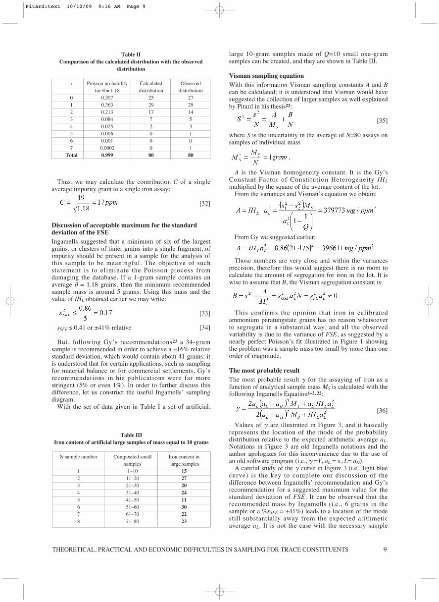
Thus, we may calculate the contribution C of a singleaverage impurity grain to a single iron assay:

[32]

Discussion of acceptable maximum for the standarddeviation of the FSEIngamells suggested that a minimum of six of the largestgrains, or clusters of tinier grains into a single fragment, ofimpurity should be present in a sample for the analysis ofthis sample to be meaningful. The objective of suchstatement is to eliminate the Poisson process fromdamaging the database. If a 1-gram sample contains anaverage � = 1.18 grains, then the minimum recommendedsample mass is around 5 grams. Using this mass and thevalue of IHL obtained earlier we may write:

[33]

sSFE ≤ 0.41 or ±41% relative [34]

But, following Gy’s recommendations23 a 34-gramsample is recommended in order to achieve a ±16% relativestandard deviation, which would contain about 41 grains; itis understood that for certain applications, such as samplingfor material balance or for commercial settlements, Gy’srecommendations in his publications were far morestringent (5% or even 1%). In order to further discuss thisdifference, let us construct the useful Ingamells’ samplingdiagram.

With the set of data given in Table I a set of artificial,

large 10-gram samples made of Q=10 small one-gramsamples can be created, and they are shown in Table III.

Visman sampling equationWith this information Visman sampling constants A and Bcan be calculated; it is understood that Visman would havesuggested the collection of larger samples as well explainedby Pitard in his thesis22:

[35]

where S is the uncertainty in the average of N=80 assays onsamples of individual mass

A is the Visman homogeneity constant. It is the Gy’sConstant Factor of Constitution Heterogeneity IHLmultiplied by the square of the average content of the lot.

From the variances and Visman’s equation we obtain:

From Gy we suggested earlier:

Those numbers are very close and within the variancesprecision, therefore this would suggest there is no room tocalculate the amount of segregation for iron in the lot. It iswise to assume that B, the Visman segregation constant is:

This confirms the opinion that iron in calibratedammonium paratungstate grains has no reason whatsoeverto segregate in a substantial way, and all the observedvariability is due to the variance of FSE, as suggested by anearly perfect Poisson’s fit illustrated in Figure 1 showingthe problem was a sample mass too small by more than oneorder of magnitude.

The most probable resultThe most probable result � for the assaying of iron as afunction of analytical sample mass MS is calculated with thefollowing Ingamells Equation1–3, 22:

[36]

Values of � are illustrated in Figure 3, and it basicallyrepresents the location of the mode of the probabilitydistribution relative to the expected arithmetic average aL.Notations in Figure 3 are old Ingamells notations and theauthor apologizes for this inconvenience due to the use ofan old software program (i.e., � =Y, aL = x, L= aH).

A careful study of the � curve in Figure 3 (i.e., light bluecurve) is the key to complete our discussion of thedifference between Ingamells’ recommendation and Gy’srecommendation for a suggested maximum value for thestandard deviation of FSE. It can be observed that therecommended mass by Ingamells (i.e., 6 grains in thesample or a %sSFE = ±41%) leads to a location of the modestill substantially away from the expected arithmeticaverage aL. It is not the case with the necessary sample

Table IIComparison of the calculated distribution with the observed

distribution

r Poisson probability Calculated Observedfor � = 1.18 distribution distribution

0 0.307 25 271 0.363 29 292 0.213 17 143 0.084 7 54 0.025 2 35 0.006 0 16 0.001 0 07 0.0002 0 1

Total 0.999 80 80

Table IIIIron content of artificial large samples of mass equal to 10 grams

N sample number Composited small Iron content insamples large samples

1 1–10 152 11–20 273 21–30 204 31–40 245 41–50 116 51–60 307 61–70 228 71–80 23



mass of 34 grams in order to obtain a %sSFE = ±16% asrecommended by Gy.

Ingamells’ gangue concentrationThe low background iron content aH estimated earlier to be4 ppm can be calculated using the mode from results fromsmall samples and the mode �2 from results from largesamples. Modes can be calculated using the harmonicmeans h1 and h2 of the data distribution of the small andlarge samples. The harmonic mean is calculated as follows:

[37]

where N is the number of samples.From Equation [36] we may write:

[38]

[39]

Then from Equations [1], [2], and [3] the low backgroundcontent aH can be calculated as follows:

[40]

Results are shown in Figure 2 and confirm the earlierestimate of 4 ppm.

If the reader is interested by the full derivation of theabove formulas, refer to Pitard’s doctoral thesis22.

ConclusionsThe key to sampling for trace amounts of a givenconstituent of interest is a thorough microscopicinvestigation of the ways such constituent is distributed ona small scale in the material to be sampled. Liberated ornot, the coarsest grains of such constituent must bemeasured and placed into the context of their average, localexpected grade. The use of Poisson statistics and thecalculation of an Ingamells’ sampling diagram can lead todefining a minimum sampling effort during the early phaseof a project. Equipped with such valuable preliminaryinformation, someone can proceed with a feasibility studyto implement a necessary sampling protocol as suggestedby the TOS, with a full understanding of what theconsequences would be if no due diligence is exercised.

Figure 2. Search for a value of the low background iron contentaH

Figure 3. Illustration of the Ingamells’ sampling diagram for iron traces in pure ammonium paratungstate ( �=Y, aL = x, L= aH)



RecommendationsAs the sampling requirements necessary to minimize thevariance of FSE as suggested in the TOS may becomecumbersome to many economists, it becomes important toproceed with preliminary tests in order to provide thenecessary information to create valuable risk assessments.The following steps, in chronological order, arerecommended:

• Carefully define data quality objectives. • Always respect the fundamental rules of sampling

correctness as explained in the TOS. This step is notnegotiable.

• Perform a thorough microscopic investigation of thematerial to be sampled in order to quantify the grainssize of the constituent of interest, liberated or not.Emphasize the size of clusters of such grains if such athing can be observed.

• Proceed with a Visman’s experiment, calculate theIngamells’ parameters, and draw an informativeIngamells’ sampling diagram.

• Show the information to executive managers who mustmake a feasibility study to justify more funds toperform a wiser and necessary approach using Gy’srequirement to minimize the variance of FSE.

References1. GY, P.M. L’Echantillonage des Minerais en Vrac

(Sampling of particulate materials). Volume 1. Revuede l’Industrie Minerale, St. Etienne, France. NumeroSpecial (Special issue, January 15, 1967).

2. GY, P.M. Sampling of Particulate Materials, Theoryand Practice. Elsevier Scientific PublishingCompany. Developments in Geomathematics 4. 1979and 1983.

3. Gy, P.M. Sampling of Heterogeneous and DynamicMaterial Systems: Theories of Heterogeneity,Sampling and Homogenizing. Amsterdam, Elsevier.1992.

4. INGAMELLS, C.O, and PITARD F. AppliedGeochemical Analysis. Wiley Interscience Division,John Wiley and Sons, Inc., New York, 1986. 733 pp.

5. INGAMELLS, C.O., and SWITZER, P. A ProposedSampling Constant for Use in Geochemical Analysis,Talanta vol. 20, 1973. pp. 547–568.

6. INGAMELLS, C.O. Control of geochemical errorthrough sampling and subsampling diagrams.Geochim. Cosmochim. Acta vol. 38, 1974. pp.1225–1237.

7. INGAMELLS, C.O. Evaluation of skewedexploration data–the nugget effect. Geochim.Cosmochim. Acta vol. 45, 1981. pp. 1209–1216.

8. PITARD, F. Pierre Gy’s Sampling Theory andSampling Practice. CRC Press, Inc., 2000 CorporateBlvd., N.W. Boca Raton, Florida 33431. Secondedition, July 1993.

9. PITARD, F. Effects of Residual Variances on theEstimation of the Variance of the Fundamental Error’,Published in a special issue by Chemometrics andIntelligent Laboratory Systems, Elsevier: 50 years ofPierre Gy’s Theory of Sampling, Proceedings: FirstWorld Conference on Sampling and Blending -(WCSB1), 2003. pp. 149–164.

10. PITARD, F. Blasthole sampling for grade control: themany problems and solutions. Sampling 2008. 27–28May 2008, Perth, Australia. The Australasian Instituteof Mining and Metallurgy. 2008.

11. PITARD, F. Sampling Correctness—A ComprehensiveGuideline. Second World Conference on Samplingand Blending 2005. The Australian Institute ofMining and Metallurgy. Publication Series No 4/2005.2005.

12. PITARD, F. Chronostatistics—A powerful,pragmatic, new science for metallurgists.Metallurgical Plant Design and Operating strategies(MetPlant 2006) 18–19 September 2006 Perth, WA.The Australasian Institute of Mining and Metallurgy.2006.

13. ESBENSEN, K.H. and MINKKINEN, P: (guest eds.).Chemometrics and Intelligent Laboratory Systems.volume 74, 1 2004. Special issue: 50 years of PierreGy’s Theory of Sampling. Proceedings: First WorldConference on Sampling and Blending (WCSB1).Tutorials on Sampling: Theory and Practice.

14. PETERSEN, L. Pierre Gy’s Theory of Sampling(TOS)—in Practice: Laboratory and IndustrialDidactics including a first foray into image analyticalsampling. ACABS Research Group. AalborgUniversity Esbjerg, Niels Bohrs Vej 8, Dk-67000Esbjerg, Denmark. Thesis submitted to theInternational Doctoral School of Science andTechnology. January 2005.

15. DAVID, M. Geostatistical Ore Reserve Estimation.Developments in Geomathematics 2 . ElsevierScientific Publishing Company. 1977.

16. FRANCOIS-BONGARCON, D. Theory of samplingand geostatistics: an intimate link. Published in aspecial issue by Chemometrics and IntelligentLaboratory Systems, Elsevier: 50 years of Pierre Gy’sTheory of Sampling, Proceedings: First WorldConference on Sampling and Blending (WCSB1),2003. pp. 143–148.

17. FRANCOIS-BONGARCON, D. The modeling of theLiberation Factor and its Calibration. Proceedings:Second World Conference on Sampling and Blending(WCSB2). Published by The AusIMM. 10-12 May2005, Sunshine Coast, Quennsland, Australia. 2005.pp. 11–13.

18. FRANCOIS-BONGARCON, D. The most commonerror in applying Gy’s formula in the Theory ofMineral Sampling, and the history of the liberationfactor. Monograph “Toward 2000”, AusImm. 2000.

19. FRANCOIS-BONGARCON, D and GY, P. The mostcommon error in applying ‘Gy’s Formula’ in thetheory of mineral sampling and the history of theLiberation factor, in Mineral Resource and OreReserve Estimation. The AusIMM Guide to GoodPractice. The Australasian Institute of Mining andMetallurgy: Melbourne. 2001. pp. 67–72

20. VISMAN, J. A General Theory of Sampling,Discussion 3, Journal of Materials, JMLSA, vol. 7,no. 3, September 1972, pp. 345–350.

21. WHITTLE, P. On stationary processes in the plane.Biometrika, vol. 41. 1954. pp. 431–449.

22. PITARD, F. Pierre Gy’s Theory of Sampling andC.O. Ingamells’ Poisson Process Approach—Pathways to Representative Sampling andAppropriate Industrial Standards. Doctoral thesis:Aalborg University, campus Esbjerg, 2009. ISBN:978-87- 7606-032-9.

23. GY, P.M. Nomogramme d’echantillonnage, SamplingNomogram, Probeanhme Nomogramm. Minerais etMetaux, Paris (Ed.). 1956.



Francis F. Pitard Francis Pitard Sampling Consultants LLC

FRANCIS F. PITARD has over 40 years of experience in the natural resources industry and atomicenergy. Accomplished in teaching short courses for Universities and companies around the world andin consulting. Versatile in applying talents in a variety of areas including nuclear chemistry, analyticalchemistry, geochemistry, and statistical process control. Outstanding expertise in all aspects ofsampling accumulated during a 20 year association with Dr. C.O. Ingamells and Dr. Pierre M. Gy.Author of many papers and two books on sampling. Francis will be presenting a 2 day samplingcourse prior to WCSB4. FRANCIS PITARD SAMPLING CONSULTANTS LLC.


keynote address: theoretical, practical and economic ... · pitard, f.f. theoretical, practical and...

Documents