key concepts and techniques in gis - city university of
TRANSCRIPT
City University of New York (CUNY) City University of New York (CUNY)
CUNY Academic Works CUNY Academic Works
Publications and Research Hunter College
2007
Key Concepts and Techniques in GIS Key Concepts and Techniques in GIS
Jochen Albrecht CUNY Hunter College
How does access to this work benefit you? Let us know!
More information about this work at: https://academicworks.cuny.edu/hc_pubs/10
Discover additional works at: https://academicworks.cuny.edu
This work is made publicly available by the City University of New York (CUNY). Contact: [email protected]

Key Concepts and Techniques in GIS
Albrecht-3572-Prelims.qxd 5/7/2007 6:10 PM Page i

Albrecht-3572-Prelims.qxd 5/7/2007 6:10 PM Page ii
Jochen Albrecht
Key Concepts and Techniques in GIS
Albrecht-3572-Prelims.qxd 5/7/2007 6:10 PM Page iii

© Jochen Albrecht 2007
First published 2007
Apart from any fair dealing for the purposes of research orprivate study, or criticism or review, as permitted under theCopyright, Designs and Patents Act, 1988, this publication maybe reproduced, stored or transmitted in any form, or by anymeans, only with the prior permission in writing of the publishers,or in the case of reprographic reproduction, in accordance with theterms of licences issued by the Copyright Licensing Agency.Enquiries concerning reproduction outside those terms should besent to the publishers.
SAGE Publications Ltd1 Oliver’s Yard55 City RoadLondon EC1Y 1SP
SAGE Publications Inc.2455 Teller RoadThousand Oaks, California 91320
SAGE Publications India Pvt LtdB1/I I Mohan Cooperative Industrial AreaMathura Road, New Delhi 110 044India
SAGE Publications Asia-Pacific Pte Ltd33 Pekin Street #02-01Far East SquareSingapore 048763
Library of Congress Control Number 2007922921
British Library Cataloguing in Publication data
A catalogue record for this book is available fromthe British Library
ISBN 978-1-4129-1015-6ISBN 978-1-4129-1016-3 (pbk)
Typeset by C&M Digitals (P) Ltd, Chennai, IndiaPrinted in Great Britain by [to be supplied]Printed on paper from sustainable resources
Albrecht-3572-Prelims.qxd 5/7/2007 6:10 PM Page iv
CONTENTS
List of Figures viiiPreface x
1 Creating Digital Data 11.1 Spatial data 21.2 Sampling 31.3 Remote sensing 51.4 Global positioning systems 71.5 Digitizing and scanning 81.6 The attribute component of geographic data 8
2 Accessing Existing Data 102.1 Data exchange 102.2 Conversion 112.3 Metadata 122.4 Matching geometries (projection and coordinate systems) 122.5 Geographic web services 14
3 Handling Uncertainty 163.1 Spatial data quality 163.2 How to handle data quality issues 18
4 Spatial Search 194.1 Simple spatial querying 194.2 Conditional querying 204.3 The query process 214.4 Selection 224.5 Background material: Boolean logic 23
5 Spatial Relationships 265.1 Recoding 265.2 Relationships between measurements 295.3 Relationships between features 31
6 Combining Spatial Data 346.1 Overlay 346.2 Spatial Boolean logic 37
Albrecht-3572-Prelims.qxd 5/7/2007 6:10 PM Page v

6.3 Buffers 386.4 Buffering in spatial search 406.5 Combining operations 406.6 Thiessen polygons 41
7 Location-Allocation 427.1 The best way 427.2 Gravity model 437.3 Location modeling 447.4 Allocation modeling 47
8 Map Algebra 488.1 Raster GIS 488.2 Local functions 508.3 Focal functions 528.4 Zonal functions 538.5 Global functions 548.6 Map algebra scripts 55
9 Terrain Modeling 569.1 Triangulated irregular networks (TINs) 579.2 Visibility analysis 589.3 Digital elevation and terrain models 599.4 Hydrological modeling 60
10 Spatial Statistics 6210.1 Geo-statistics 62
10.1.1 Inverse distance weighting 6210.1.2 Global and local polynomials 6310.1.3 Splines 6410.1.4 Kriging 66
10.2 Spatial analysis 6710.2.1 Geometric descriptors 6710.2.2 Spatial patterns 6910.2.3 The modifiable area unit problem (MAUP) 7110.2.4 Geographic relationships 72
11 Geocomputation 7311.1 Fuzzy reasoning 7311.2 Neural networks 7511.3 Genetic algorithms 7611.4 Cellular automata 7711.5 Agent-based modeling systems 78
vi CONTENTS
Albrecht-3572-Prelims.qxd 5/7/2007 6:10 PM Page vi

12 Epilogue: Four-Dimensional Modeling 81
Glossary 84References 88Index 91
CONTENTS vii
Albrecht-3572-Prelims.qxd 5/7/2007 6:10 PM Page vii

LIST OF FIGURES
Figure 1 Object vs. field view (vector vs. raster GIS). 3Figure 2 Couclelis’ ‘Hierarchical Man’ 4Figure 3 Illustration of variable source problem 5Figure 4 Geographic relationships change according to scale 6
Figure 5 One geography but many different maps 11Figure 6 Subset of a typical metadata tree 13Figure 7 The effect of different projections 14
Figure 8 Simple query by location 20Figure 9 Conditional query or query by (multiple) attributes 21Figure 10 The relationship between spatial and attribute query 22Figure 11 Partial and complete selection of features 23Figure 12 Using one set of features to select another set 24Figure 13 Simple Boolean logic operations 24
Figure 15 Recoding as simplification 27Figure 14 Typical soil map 27Figure 17 Recoding to derive new information 28Figure 16 Recoding as a filter operation 28Figure 19 Simple (top row) and complex (bottom row) geometries 30Figure 18 Four possible spatial relationships in a pixel world 30Figure 20 Pointer structure between tables of feature geometries 31Figure 22 Topological relationships between features 32Figure 21 Part of the New York subway system 32
Figure 24 Overlay as a coincidence function 35Figure 23 Schematics of a polygon overlay operation 35Figure 25 Overlay with multiple input layers 36Figure 26 Spatial Boolean logic 37Figure 27 The buffer operation in principle 38Figure 29 Corridor function 39Figure 28 Inward or inverse buffer 39Figure 30 Surprise effects of buffering affecting towns
outside a flood zone 40Figure 31 Thiessen polygons (pronounced the
German way as ‘ee’) 41
Albrecht-3572-Prelims.qxd 5/7/2007 6:10 PM Page viii
Figure 32 Areas of influence determining the reachof gravitational pull 44
Figure 34 Weber’s triangle 45Figure 33 Von Thünen’s agricultural zones around a market 45Figure 35 Christaller’s Central Place theory 46Figure 36 Origin-destination matrix 47
Figure 37 The spatial scope of raster operations 49Figure 38 Raster organization and cell position addressing 49Figure 39 Zones of raster cells 50Figure 40 Local function 51Figure 41 Multiplication of a raster layer by a scalar 51Figure 43 Focal function 52Figure 42 Multiplying one layer by another one 52Figure 44 Averaging neighborhood function 53Figure 45 Zonal function 54Figure 46 Value grids as spatial lookup tables 55
Figure 47 Three ways to represent the third dimension 56Figure 48 Construction of a TIN 57Figure 49 Viewshed 58Figure 50 Derivation of slope and aspect 59Figure 51 Flow accumulation map 60
Figure 52 Inverse distance weighting 63Figure 54 Local and global polynomials 64Figure 53 Polynomials of first and second order 64Figure 56 Application of splines to surfaces 65Figure 55 Historical use of splines 65Figure 57 Exact and inexact interpolators 66Figure 58 Geometric mean 68Figure 59 Geometric mean and geometric median 69Figure 61 Shape measures 70Figure 60 Standard deviational ellipse 70Figure 62 Joint count statistic 71
Figure 63 Shower tab illustrating fuzzy notionsof water temperature 74
Figure 64 Schematics of a single neuron, the buildingblock of an artificial neural network 75
Figure 65 Genetic algorithms are mainly applied when the modelbecomes too complicated to be solved deterministically 77
Figure 66 Principles of genetic algorithms 78
LIST OF FIGURES ix
Albrecht-3572-Prelims.qxd 5/7/2007 6:10 PM Page ix

PREFACE
GIS has been coming of age. Millions of people use one GIS or another every day,and with the advent of Web 2.0 we are promised GIS functionality on virtually everydesktop and web-enabled cellphone. GIS knowledge, once restricted to a few insid-ers working with minicomputers that, as a category, don’t exist any more, hasproliferated and is bestowed on students at just about every university and increasinglyin community colleges and secondary schools. GIS textbooks abound and in thecourse of twenty years have moved from specialized topics (Burrough 1986) togeneral-purpose textbooks (Maantay and Ziegler 2006). With such a well-informeduser audience, who needs yet another book on GIS?
The answer is two-fold. First, while there are probably millions who use GIS,there are far fewer who have had a systematic introduction to the topic. Many areself-trained and good at the very small aspect of GIS they are doing on an everydaybasis, but they lack the bigger picture. Others have learned GIS somewhat systemat-ically in school but were trained with a particular piece of software in mind – and inany case were not made aware of modern methods and techniques. Mostly, however,this book addresses all the others: those who have to distinguish between, on the onehand, the claims and promises of software vendors and job applicants alike, and onthe other hand the realities and prospects of the marketplace. In other words, thisbook is aimed at decision-makers of all kinds – those who need to decide whetherthey should invest in GIS or wait for GIS functionality in Google Earth (VirtualEarth if you belong to the other camp), as well as personnel managers who need toread up on the topic in preparation for interviewing a posse of job applicants.
This book is indebted to two role models. In the 1980s, Sage published a tremen-dously useful series of little green paperbacks that reviewed quantitative methods,mostly for the social sciences. They were concise, cheap (as in extremely good quality/price ratio), and served students and practitioners alike. If this little volume that youare now holding contributes to the revival of this series, then I consider my task tobe fulfilled. The other role model is an unsung hero, mostly because it served sucha small readership. The CATMOG (Concepts and Techniques in ModernGeography) series fulfills the same set of criteria and I guess it is no coincidence thatit too has been published by Sage. CATMOG is now unfortunately out of print butdeserves to be promoted to the modern GIS audience at large, which as I pointed outearlier is just about everybody. With these two exemplars of the publishing pantheonin house, is it a wonder that I felt honored to be invited to write this volume? Mykudos goes to the unknown editors of these two series.
<author signature>
Albrecht-3572-Prelims.qxd 5/7/2007 6:10 PM Page x
The creation of spatial data is a surprisingly underdeveloped topic in GIS literature.Part of the problem is that it is a lot easier to talk about tangibles such as data as acommodity, and digitizing procedures, than to generalize what ought to be the veryfirst step: an analysis of what is needed to solve a particular geographic question.Social sciences have developed an impressive array of methods under the umbrellaof research design, originally following the lead of experimental design in the natu-ral sciences but now an independent body of work that gains considerably moreattention than its counterpart in the natural sciences (Mitchell and Jolley 2001).
For GIScience, however, there is a dearth of literature on the proper developmentof (applied) research questions; and even outside academia there is no vendor-independent guidance for the GIS entrepreneur on setting up the databases that off-the-shelf software should be applied to. GIS vendors try their best to provide theircustomers with a starter package of basic data; but while this suffices for training ortutorial purposes, it cannot substitute for in-house data that is tailored to the needsof a particular application area.
On the academic side, some of the more thorough introductions to GIS (e.g.Chrisman 2002) discuss the history of spatial thought and how it can be expressedas a dialectic relationship between absolute and relative notions of space and time,which in turn are mirrored in the two most common spatial representations of rasterand vector GIS. This is a good start in that it forces the developer of a new GIS data-base to think through the limitations of the different ways of storing (and acquiring)spatial data, but it still provides little guidance.
One of the reasons for the lack of literature – and I dare say academic research –is that far fewer GIS would be sold if every potential buyer knew how much work isinvolved in actually getting started with one’s own data. Looking from the ivorytower, there are ever fewer theses written that involve the collection of relevant databecause most good advisors warn their mentees about the time involved in that taskand there is virtually no funding of basic research for the development of new meth-ods that make use of new technologies (with the exception of remote sensing wherethis kind of research is usually funded by the manufacturer). The GIS trade maga-zines of the 1980s and early 90s were full of eye-witness reports of GIS projectsrunning over budget; and a common claim back then was that the development of thedatabase, which allows a company or regional authority to reap the benefitsof the investment, makes up approximately 90% of the project costs. Anecdotalevidence shows no change in this staggering character of GIS data assembly(Hamil 2001).
1 CREATING DIGITAL DATA
Albrecht-3572-Ch-01.qxd 5/7/2007 6:16 PM Page 1

So what are the questions that a prospective GIS manager should look into beforeembarking on a GIS implementation? There is no definitive list, but the followingquestions will guide us through the remainder of this chapter.
• What is the nature of the data that we want to work with?• Is it quantitative or qualitative?• Does it exist hidden in already compiled company data?• Does anybody else have the data we need? If yes, how can we get hold of it? See
also Chapter 2.• What is the scale of the phenomenon that we try to capture with our data?• What is the size of our study area?• What is the resolution of our sampling?• Do we need to update our data? If yes, how often?• How much data do we need, i.e. a sample or a complete census?• What does it cost? An honest cost–benefit analysis can be a real eye-opener.
Although by far the most studied, the first question is also the most difficult one(Gregory 2003). It touches upon issues of research design and starts with a set ofgoals and objectives for setting up the GIS database. What are the questions that wewould like to get answered with our GIS? How immutable are those questions – inother words, how flexible does the setup have to be? It is a lot easier (and hencecheaper) to develop a database to answer one specific question than to develop a gen-eral-purpose system. On the other hand, it usually is very costly and sometimes evenimpossible to change an existing system to answer a new set of questions.
The next step is then to determine what, in an ideal world, the data would looklike that answers our question(s). Our world is not ideal and it is unlikely that wewill gather the kind of data prescribed in this step, but it is interesting to understandthe difference between what we would like to have and what we actually get.Chapter 3 will expand on the issues related to imperfect data.
1.1 Spatial data
In its most general form, geographic data can be described as any kind of data thathas a spatial reference. A spatial reference is a descriptor for some kind of location,either in direct form expressed as a coordinate or an address or in indirect form rel-ative to some other location. The location can (1) stand for itself or (2) be part of aspatial object, in which case it is part of the boundary definition of that object.
In the first instance, we speak of a field view of geographic information becauseall the attributes associated with that location are taken to accurately describeeverything at that very position but are to be taken less seriously the further we getaway from that location (and the closer we can to another location).
The second type of locational reference is used for the description of geographicobjects. The position is part of a geometry that defines the boundary of that object.
2 KEY CONCEPTS AND TECHNIQUES IN GIS
Albrecht-3572-Ch-01.qxd 5/7/2007 6:16 PM Page 2

The attributes associated with this piece of geographic data are supposed to be validfor all coordinates that are part of the geographic object. For example, if we have theattribute ‘population density’ for a census unit, then the density value is assumed tobe valid throughout this unit. This would obviously be unrealistic in the case wherea quarter of this unit is occupied by a lake, but it would take either lots of auxiliaryinformation or sophisticated techniques to deal with this representational flaw.Temporal aspects are treated just as another attribute. GIS have only very limitedabilities to reason about temporal relationships.
This very general description of spatial data is slightly idealistic (Couclelis 1992). Inpractice, most GIS distinguish strictly between the two types of spatial perspectives – thefield view that is typically represented using raster GIS, versus the object viewexemplified by vector GIS (see Figure 1). The sets of functionalities differ consider-ably depending on which perspective is adopted.
1.2 Sampling
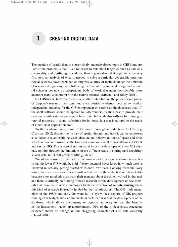
But before we get there, we will have to look at the relationship between the real-world question and the technological means that we have to answer it. HelenCouclelis (1982) described this process of abstracting from the world that we live into the world of GIS in the form of a ‘hierarchical man’ (see Figure 2). GIS store theirspatial data in a two-dimensional Euclidean geometry representation, and while evenspatial novices tend to formalize geographic concepts as simple geometry, we allrealize that this is not an adequate representation of the real world. The hierarchicalman illustrates the difference between how we perceive and conceptualize the worldand how we represent it on our computers. This in turn then determines the kinds ofquestions (procedures) that we can ask of our data.
This explains why it is so important to know what one wants the GIS to answer.It starts with the seemingly trivial question of what area we should collect the datafor – ‘seemingly’ because, often enough, what we observe for one area is influencedby factors that originate from outside our area of interest. And unless we have
CREATING DIGITAL DATA 3
32.3
x,y
x,yx,y
x,y
x,yx,yx,y
x,yx,y
x,yx,yx,y
x,y x,yx,y
40.841.8
43.0 36.136.2
32.631.1 30.4 31.2 30.6
32.733.5
33.6
35.1 33.034.6
33.131.2
34.9
Figure 1 Object vs. field view (vector vs. raster GIS).
Albrecht-3572-Ch-01.qxd 5/7/2007 6:16 PM Page 3
complete control over all aspects of all our data, we might have to deal with bound-aries that are imposed on us but have nothing to do with our research question (themodifiable area unit problem, or MAUP, which we will revisit in Chapter 10). Anexample is street crime, where our outer research boundary is unlikely to be relatedto the city boundary, which might have been the original research question, andwhere the reported cases are distributed according to police precincts, which in turnwould result in different spatial statistics if we collected our data by precinct ratherthan by address (see Figure 3).
In 99% of all situations, we cannot conduct a complete census – we cannot inter-view every customer, test every fox for rabies, or monitor every brown field (formerindustrial site). We then have to conduct a sample and the techniques involved areradically different depending on whether we assume a discrete or continuous distri-bution and what we believe the causal factors to be. We deal with a chicken-and-eggdilemma here because the better our understanding of the research question, themore specific and hence appropriate can be our sampling technique. Our needs,however, are exactly the other way around. With a generalist (‘if we don’t know any-thing, let’s assume random distribution’) approach, we are likely to miss the crucialevents that would tell us more about the unknown phenomenon (be it West Nile virusor terrorist chatter).
4 KEY CONCEPTS AND TECHNIQUES IN GIS
H1 Real Space
H2 Conditioned Space
Use Space
Rated Space
Adapted Space
Euclidean Space
H3
H4
H5
Standard SpaceHK-1
HK
Figure 2 Couclelis’ ‘Hierarchical Man’
Albrecht-3572-Ch-01.qxd 5/7/2007 6:16 PM Page 4

Most sampling techniques apply to so-called point data; i.e., individual locationsare sampled and assumed to be representative for their immediate neighborhood.Values for non-sampled locations are then interpolated assuming continuous distri-butions. The interpolation techniques will be discussed in Chapter 10. Currentlyunresolved are the sampling of discrete phenomena, and how to deal with spatialdistributions along networks, be they river or street networks.
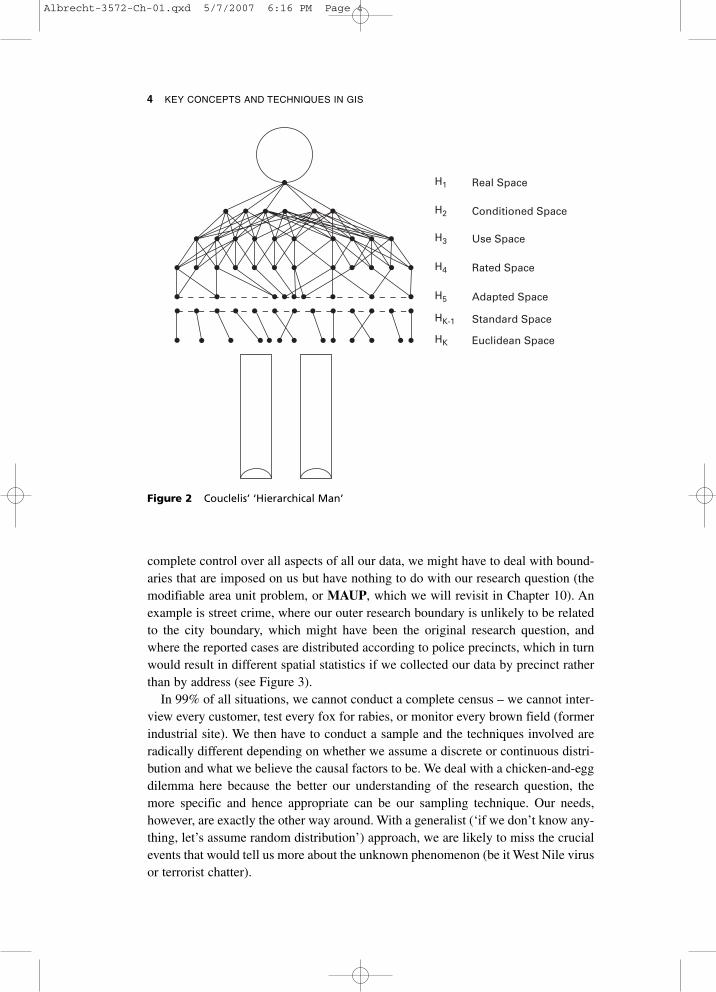
Surprisingly little attention has been paid to the appropriate scale for sampling.A neighborhood park may be the world to a squirrel but is only one of many possi-ble hunting grounds for the falcon nesting on a nearby steeple (see Figure 4). Everygeographic phenomenon can be studied at a multitude of scales but usually only asmall fraction of these is pertinent to the question at hand. As mentioned earlier,knowing what one is after goes a long way in choosing the right approach.
Given the size of the study area, the assumed form of spatial distribution andscale, and the budget available, one eventually arrives at a suitable spatial resolution.However, this might be complicated by the fact that some spatial distributionschange over time (e.g. people on the beach during various seasons). In the end, onehas to make sure that one’s sampling represents, or at least has a chance to represent,the phenomenon that the GIS is supposed to serve.
1.3 Remote sensing
Without wasting too much time on the question whether remotely sensed data is pri-mary or secondary data, a brief synopsis of the use of image analysis techniques asa source for spatial data repositories is in order. Traditionally, the two fields of GISand remote sensing were cousins who acknowledged each other’s existence butotherwise stayed clearly away from each other. The widespread availability of remotelysensed data and especially pressure from a range of application domains have forcedthe two communities to cross-fertilize. This can be seen in the added functionalitiesof both GIS and remote sensing packages, although the burden is still on the user toextract information from remotely sensed data.
CREATING DIGITAL DATA 5
Census Voting District Police
Armed Robbery Assaults
Figure 3 Illustration of variable source problem
Albrecht-3572-Ch-01.qxd 5/7/2007 6:16 PM Page 5
Originally, GIS and remote sensing data were truly complimentary by adding con-text to the respective other. GIS data helped image analysts to classify otherwiseambiguous pixels, while imagery used as backdrop to highly specialized vector dataprovides orientation and situational setting. Truly integrated software that mixes andmatches raster, vector and image data for all kinds of GIS functions does not exist;at best, some raster analytical functions take vector data as determinants of process-ing boundaries. To make full use of remotely sensed data, the GIS user needs tounderstand the characteristics of a wide range of sensors and what kind of manipu-lation the imagery has undergone before it arrives on the user’s desk.
Remotely sensed data is a good example for the field view of spatial informationdiscussed earlier. For each location we are given a value, called digital number(DN), usually in the range from 0 to 255, sometimes up to 65,345. These digitalnumbers are visualized by different colors on the screen but the software works withDN values rather than with colors. The satellite or airborne sensors have different
6 KEY CONCEPTS AND TECHNIQUES IN GIS
Figure 4 Geographic relationships change according to scale
Albrecht-3572-Ch-01.qxd 5/7/2007 6:16 PM Page 6

sensitivities in a wide range of the electromagnetic spectrum, and one aspect that isconfusing for many GIS users is that the relationship between a color on the screen anda DN representing a particular but very small range of the electromagnetic spectrum isarbitrary. This is unproblematic as long as we leave the analysis entirely to thecomputer – but there is only a very limited range of tasks that can be performed auto-matically. In all other instances we need to understand what a screen color stands for.
Most remotely sensed data comes from so-called passive sensors, where the sen-sor captures reflections of energy of the earth’s surface that originally comes fromthe sun. Active sensors on the other hand send their own signal and allow the imageanalyst to make sense of the difference between what was sent off and what bouncesback from the ‘surface’. In either instance, the word surface refers either to the topo-graphic surface or to parts in close vicinity, such as leaves, roofs, minerals or waterin the ground. Early generations of sensors captured reflections predominantly in asmall number of bands of the visible (to the human eye) and infrared ranges, but thenumber of spectral bands as well as their distance from the visible range hasincreased. In addition, the resolution of images has improved from multiple kilome-ters to fractions of a meter (or centimeters in the case of airborne sensors).
With the right sensor, software and expertise of the operator we can now useremotely sensed data to distinguish not only various kinds of crops but also theirmaturity, response to drought conditions or mineral deficiencies. We can detectburied archaeological sites, do mineral exploration, and measure the height ofwaves. But all of these require a thorough understanding of what each sensor can andcannot capture as well as what conceptual model image analysts use to draw theirconclusions from the digital numbers mentioned above. The difference between aca-demic theory and operational practice is often discouraging. This author, forinstance, searched in vain for imagery that helps to discern the vanishing rate of Irishbogs because for many years there happened to be no coincidence between cloud-less days and a satellite over these areas on a clear day.
On the upside, once one has the kind of remotely sensed data that the GIS practi-tioner is looking for and some expertise in manipulating it (see Chapter 8), then theoptions for improved GIS applications are greatly enhanced.
1.4 Global positioning systems
Usually, when we talk about remotely sensed data, we are referring to imagery – thatis, a file that contains reflectance values for many points covering a given rectangulararea. The global positioning system (GPS) is also based on satellite data, but the dataconsists of positions only – there is no attribute information other than some metadataon how the position was determined. Another difference is that GPS data can be col-lected on a continuing basis, which helps to collect not just single positions but alsoroute data. In other words, while a remotely sensed image contains data about a lot ofneighboring locations that gets updated on a daily to yearly basis, GPS data potentiallyconsist of many irregularly spaced points that are separated by seconds or minutes.
CREATING DIGITAL DATA 7
Albrecht-3572-Ch-01.qxd 5/7/2007 6:16 PM Page 7
As of 2006, there was only one easily accessible GPS world-wide. The Russiansystem as well as alternative military systems are out of reach of the typical GISuser, and the planned civilian European system will not be functional for a numberof years. Depending on the type of receiver, ground conditions, and satellite con-stellations, the horizontal accuracy of GPS measurements lies between a few cen-timeters and a few hundred meters, which is sufficient for most GIS applications(however, buyer beware: it is never as good as vendors claim).
GPS data is mainly used to attach a position to field data – that is, to spatializeattribute measurements taken in the field. It is preferable for the two types of meas-urement to be taken concurrently because this decreases the opportunity for errors inmatching measurements with their corresponding position. GPS data is increasinglyaugmented by a new version of triangulating one’s position that is based on cell-phone signals (Bryant 2005). Here, the three or more satellites are either replaced orpreferably added to by cellphone towers. This increases the likelihood of having acontinuous signal, especially in urban areas, where buildings might otherwise dis-rupt GPS reception. Real-time applications especially benefit from the ability totrack moving objects this way.
1.5 Digitizing and scanning
Most spatial legacy data exists in the form of paper maps, sketches or aerial photo-graphs. And although most newly acquired data comes in digital format, legacy dataholds potentially enormous amounts of valuable information. The term digitizing isusually applied to the use of a special instrument that allows interactive tracing ofthe outline of features on an analogue medium (mostly paper maps). This is in con-trast to scanning, where an instrument much like a photocopying or fax machinecaptures a digital image of the map, picture or sketch. The former creates geometriesfor geographic objects, while the latter results in a picture much like early uses ofimagery to provide a backdrop for pertinent geometries.
Nowadays, the two techniques have merged in what is sometimes called on-screenor heads-up digitizing, where a scanned image is loaded into the GIS and the oper-ator then traces the outline of objects of their choice on the screen. In any case, andparallel to the use of GPS measurements, the result is a file of mere geometries,which then have to be linked with the attribute data describing each geographicobject. Outsiders keep being surprised how little the automatic recognition of objectshas been advanced and hence how much labor is still involved in digitizing or scan-ning legacy data.
1.6 The attribute component of geographic data
Most of the discussion above concerns the geometric component of geographicinformation. This is because it is the geometric aspects that make spatial data
8 KEY CONCEPTS AND TECHNIQUES IN GIS
Albrecht-3572-Ch-01.qxd 5/7/2007 6:16 PM Page 8

special. Handling of the attributes is pretty much the same as for general-purposedata handling, say in a bank or a personnel department. Choice of the correctattribute, questions of classification, and error handling are all important topics; butin most instances, a standard textbook on database management would provide anadequate introduction.
More interesting are concerns arising from the combination of attributes andgeometries. In addition to the classical mismatch, we have to pay special attention toa particular geographic form of ecological fallacy. Spatial distributions are hardlyever uniform within a unit of interest, nor are they independent of scale.
CREATING DIGITAL DATA 9
Albrecht-3572-Ch-01.qxd 5/7/2007 6:16 PM Page 9

Most GIS users will start using their systems by accessing data compiled either bythe GIS vendor by or the organization for which they work. Introductory tutorialstend to gloss over the amount of work involved even if the data does not have to becreated from scratch. Working with existing data starts with finding what’s out thereand what can be rearranged easily to fulfill one’s data requirements. We are currentlyexperiencing a sea change that comes under the buzz word of interoperability.GISystems and the data that they consist of used to be insular enterprises, whereeven if two parties were using the same software, the data had to exported to anexchange format. Nowadays different operating systems do not pose any seriouschallenge to data exchange any more, and with ubiquitous WWW access, theremaining issues are not as much technical in nature.
2.1 Data exchange
Following the logic of geographic data structure outlined in Chapter 1, dataexchange has to deal with two dichotomies, the common (though not necessary) dis-tinction between geometries and attributes, and the difference between the geo-graphic data on the one hand and its cartographic representation on the other.
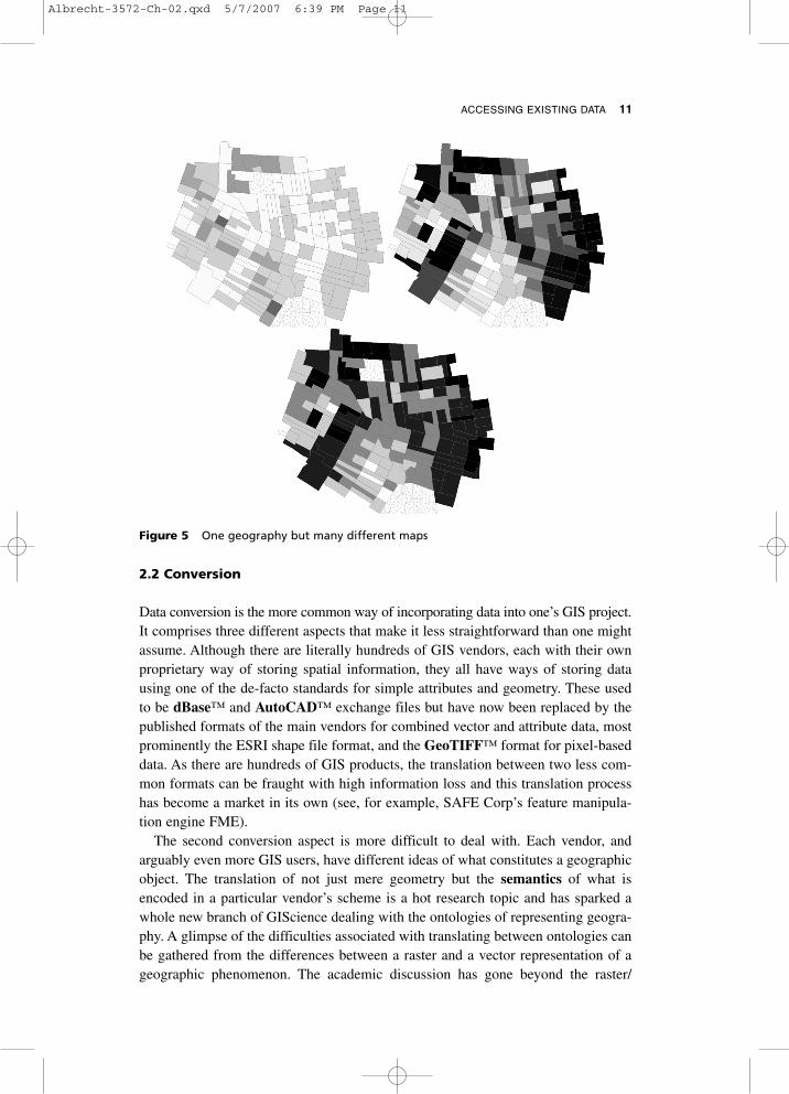
Let us have a closer look at the latter issue. Geographic data is stored as a combina-tion of locational, attribute and possibly temporal components, where the locational partis represented by a reference to a virtual position or a boundary object. This locationalpart can be represented in many different ways – usually referred to as the mapping ofa given geography. This mapping is often the result of a very laborious process of com-bining different types of geographic data, and if successful, tells us a lot more than theoriginal tables that it is made up of (see Figure 5). Data exchange can then be seenas (1) the exchange of the original geography, (2) the exchange of only the mapgraphics – that is, the map symbols and their arrangement, or (3) the exchange of both.The translation from geography to map is a proprietary process, in addition to the user’sdecisions of how to represent a particular geographic phenomenon.
The first thirty years of GIS saw the exchange mainly of ASCII files in a propri-etary but public format. These exchange files are the result of an export operationand have to be imported rather than directly read into the second system. Recentstandardization efforts led to a slightly more sophisticated exchange format based onthe Web’s extended markup language XML. The ISO standards, however, cover onlya minimum of commonality across the systems and many vendor-specificfeatures are lost during the data exchange process.
2 ACCESSING EXISTING DATA
Albrecht-3572-Ch-02.qxd 5/7/2007 6:39 PM Page 10
ACCESSING EXISTING DATA 11
2.2 Conversion
Data conversion is the more common way of incorporating data into one’s GIS project.It comprises three different aspects that make it less straightforward than one mightassume. Although there are literally hundreds of GIS vendors, each with their ownproprietary way of storing spatial information, they all have ways of storing datausing one of the de-facto standards for simple attributes and geometry. These usedto be dBase™ and AutoCAD™ exchange files but have now been replaced by thepublished formats of the main vendors for combined vector and attribute data, mostprominently the ESRI shape file format, and the GeoTIFF™ format for pixel-baseddata. As there are hundreds of GIS products, the translation between two less com-mon formats can be fraught with high information loss and this translation processhas become a market in its own (see, for example, SAFE Corp’s feature manipula-tion engine FME).
The second conversion aspect is more difficult to deal with. Each vendor, andarguably even more GIS users, have different ideas of what constitutes a geographicobject. The translation of not just mere geometry but the semantics of what isencoded in a particular vendor’s scheme is a hot research topic and has sparked awhole new branch of GIScience dealing with the ontologies of representing geogra-phy. A glimpse of the difficulties associated with translating between ontologies canbe gathered from the differences between a raster and a vector representation of ageographic phenomenon. The academic discussion has gone beyond the raster/
Figure 5 One geography but many different maps
Albrecht-3572-Ch-02.qxd 5/7/2007 6:39 PM Page 11
12 KEY CONCEPTS AND TECHNIQUES IN GIS
vector debate, but at the practical level this is still the cause of major headaches,which can be avoided only if all potential users of a GIS dataset are involved in theoriginal definition of the database semantics. For example, the description of aspecific shoal/sandbank depends on whether one looks at it as an obstacle (asdepicted on a nautical chart) or as a seal habitat, which requires parts to be abovewater at all times but defines a wider buffer of no disturbance than is necessary forpurely navigational purposes.
The third aspect has already been touched upon in the section on data exchange –the translation from geography to map data. In addition to the semantics ofgeographic features, a lot of effort goes into the organization of spatial data. Howcomplex can individual objects be? Can different vector types be mixed, or vectorand raster definitions of a feature? What about representations at multiple scales? Isthe projection part of the geographic data or the map (see next section)? There aremany ways to skin a cat. And these ways are virtually impossible to mirror in a con-version from one system to another. One solution is to give up on the exchange ofthe underlying geographic data and to use a desktop publishing or the web-basedSVG format to convert data from and to. These provide users with the opportunityto alter the graphical representation. The ubiquitous PDF format, on the other hand,is convenient because it allows exchanging maps regardless of the recipient’s outputdevice but it is a dead end because it cannot be converted into meaningful map orgeography data.
2.3 Metadata
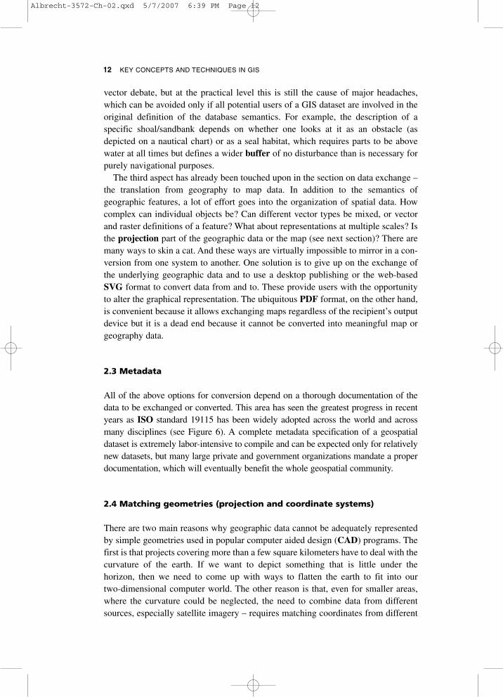
All of the above options for conversion depend on a thorough documentation of thedata to be exchanged or converted. This area has seen the greatest progress in recentyears as ISO standard 19115 has been widely adopted across the world and acrossmany disciplines (see Figure 6). A complete metadata specification of a geospatialdataset is extremely labor-intensive to compile and can be expected only for relativelynew datasets, but many large private and government organizations mandate a properdocumentation, which will eventually benefit the whole geospatial community.
2.4 Matching geometries (projection and coordinate systems)
There are two main reasons why geographic data cannot be adequately representedby simple geometries used in popular computer aided design (CAD) programs. Thefirst is that projects covering more than a few square kilometers have to deal with thecurvature of the earth. If we want to depict something that is little under thehorizon, then we need to come up with ways to flatten the earth to fit into ourtwo-dimensional computer world. The other reason is that, even for smaller areas,where the curvature could be neglected, the need to combine data from differentsources, especially satellite imagery – requires matching coordinates from different
Albrecht-3572-Ch-02.qxd 5/7/2007 6:39 PM Page 12
coordinate systems. The good news is that most GIS these days relieve us from theburden of translating between the hundreds of projections and coordinate systems.The bad news is that we still need to understand how this works to ask the right ques-tions in case the metadata fails to report on these necessities.
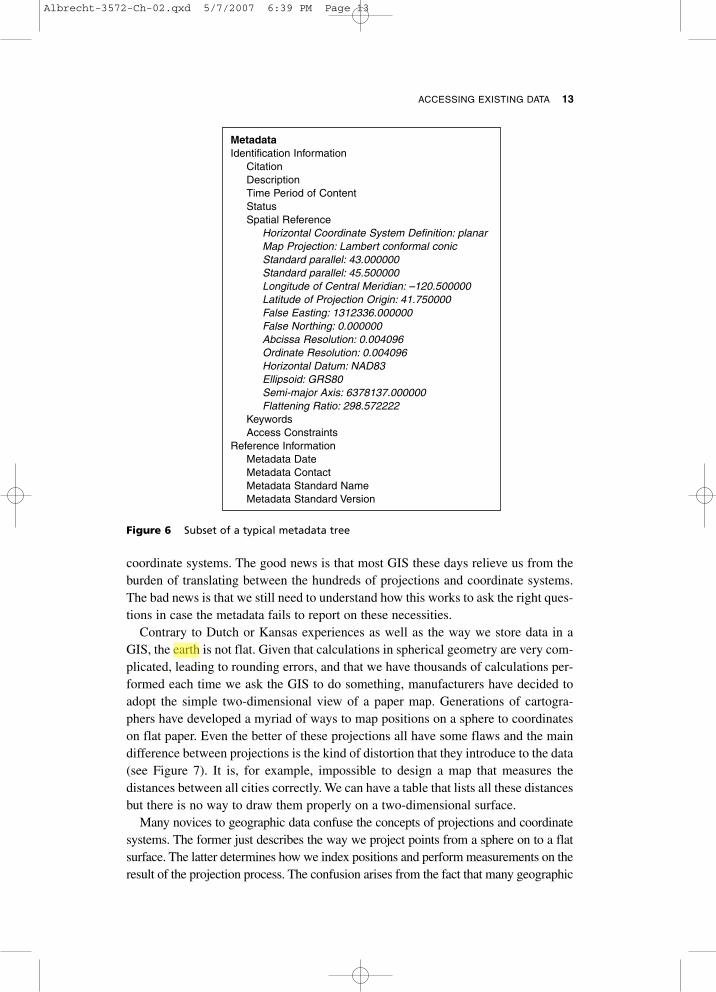
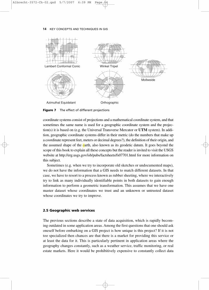
Contrary to Dutch or Kansas experiences as well as the way we store data in aGIS, the earth is not flat. Given that calculations in spherical geometry are very com-plicated, leading to rounding errors, and that we have thousands of calculations per-formed each time we ask the GIS to do something, manufacturers have decided toadopt the simple two-dimensional view of a paper map. Generations of cartogra-phers have developed a myriad of ways to map positions on a sphere to coordinateson flat paper. Even the better of these projections all have some flaws and the maindifference between projections is the kind of distortion that they introduce to the data(see Figure 7). It is, for example, impossible to design a map that measures thedistances between all cities correctly. We can have a table that lists all these distancesbut there is no way to draw them properly on a two-dimensional surface.
Many novices to geographic data confuse the concepts of projections and coordinatesystems. The former just describes the way we project points from a sphere on to a flatsurface. The latter determines how we index positions and perform measurements on theresult of the projection process. The confusion arises from the fact that many geographic
ACCESSING EXISTING DATA 13
Figure 6 Subset of a typical metadata tree
MetadataIdentification Information
CitationDescriptionTime Period of ContentStatusSpatial Reference
Horizontal Coordinate System Definition: planarMap Projection: Lambert conformal conicStandard parallel: 43.000000Standard parallel: 45.500000Longitude of Central Meridian: –120.500000Latitude of Projection Origin: 41.750000False Easting: 1312336.000000False Northing: 0.000000Abcissa Resolution: 0.004096Ordinate Resolution: 0.004096Horizontal Datum: NAD83Ellipsoid: GRS80Semi-major Axis: 6378137.000000Flattening Ratio: 298.572222
KeywordsAccess Constraints
Reference InformationMetadata DateMetadata ContactMetadata Standard NameMetadata Standard Version
Albrecht-3572-Ch-02.qxd 5/7/2007 6:39 PM Page 13
coordinate systems consist of projections and a mathematical coordinate system, and thatsometimes the same name is used for a geographic coordinate system and the projec-tion(s) it is based on (e.g. the Universal Transverse Mercator or UTM system). In addi-tion, geographic coordinate systems differ in their metric (do the numbers that make upa coordinate represent feet, meters or decimal degrees?), the definition of their origin, andthe assumed shape of the earth, also known as its geodetic datum. It goes beyond thescope of this book to explain all these concepts but the reader is invited to visit the USGSwebsite at http://erg.usgs.gov/isb/pubs/factsheets/fs07701.html for more information onthis subject.
Sometimes (e.g. when we try to incorporate old sketches or undocumented maps),we do not have the information that a GIS needs to match different datasets. In thatcase, we have to resort to a process known as rubber sheeting, where we interactivelytry to link as many individually identifiable points in both datasets to gain enoughinformation to perform a geometric transformation. This assumes that we have onemaster dataset whose coordinates we trust and an unknown or untrusted datasetwhose coordinates we try to improve.
2.5 Geographic web services
The previous sections describe a state of data acquisition, which is rapidly becom-ing outdated in some application areas. Among the first questions that one should askoneself before embarking on a GIS project is how unique is this project? If it is nottoo specialized then chances are that there is a market for providing this service orat least the data for it. This is particularly pertinent in application areas where thegeography changes constantly, such as a weather service, traffic monitoring, or realestate markets. Here it would be prohibitively expensive to constantly collect data
14 KEY CONCEPTS AND TECHNIQUES IN GIS
Figure 7 The effect of different projections
Lambert Conformal Conic Winkel Tripel
Mollweide
OrthographicAzimuthal Equidstant
Albrecht-3572-Ch-02.qxd 5/7/2007 6:39 PM Page 14

for just one application and one should look for either data or if one is lucky eventhe analysis results on the web.
Web-based geographic data provision has come a long (and sometimes unex-pected) way. In the 1990s and the first few years of the new millennium, the empha-sis was on FTP servers and web portals that provided access to either public domaindata (the USGS and US Census Bureau played a prominent role in the US) or tocommercial data, most commonly imagery. Standardization efforts, especially thoseaimed at congruence with other IT standards, helped geographic services to becomemainstream. Routing services (like it or not, MapQuest has become a householdname for what geography is about), neighborhood searches such as local.yahoo.com,and geodemographics have helped to catapult geographic web services out of theacademic realm and into the marketplace. There is an emerging market for non-GISapplications that are yet based on the provision of decentralized geodata in thewidest sense. Many near real-time applications such as sending half a million vol-unteers on door-to-door canvassing during the 2004 presidential elections in the US,the forecast of avalanche risks and subsequent day-to-day operation of ski lifts in theEuropean Alps, or the coordination of emergency management efforts during the2004 tsunami have only been possible because the interoperability of web services.
The majority of web services are commercial, accessible only for a fee (commer-cial providers might have special provisions in case of emergencies). As this is a verynew market, the rates are fluctuating and negotiable but can be substantial if thereare many (as in millions) individual queries. The biggest potential lies in the emer-gence of middle-tier applications not aimed at the end user that are based on raw dataand transform these to be combined with other web services. Examples includeconcierge services that map attractions around hotels with continuously updatedrestaurant menus, department store sales, cinema schedules, etc., or a nature conser-vation website that continuously maps GPS locations of collared elephants in rela-tionship to updated satellite imagery rendered in a 3-D landscape that changesaccording to the direction of the track. In some respect, this spells the demise of GISas we know it because the tasks that one would usually perform in a GIS are nowexecuted on a central server that combines individual services the same way that anend consumer used to combine GIS functions. Similar to the way that a Unix shellscript programmer combines little programs to develop highly customized applica-tions, web services application programmers now combine traditional GIS function-ality with commercial services (like the one that performs a secure credit cardtransaction) to provide highly specialized functionality at a fraction of the price of aGIS installation.
This form of outsourcing can have great economical benefits and as in the case ofemergency applications may be the only way to compile crucial information at sortnotice. But it comes at the price of losing control over how data is combined. Thenext chapter will deal with this issue of quality control in some detail.
ACCESSING EXISTING DATA 15
Albrecht-3572-Ch-02.qxd 5/7/2007 6:39 PM Page 15

The only way to justifiably be confident about the data one is working with is tocollect all the primary data oneself and to have complete control over all aspects ofacquisition and processing. In the light of the costs involved in creating or accessingexisting data this is not a realistic proposition for most readers.
GIS own their right of existence to their use in a larger spatial decision-makingprocess. By basing our decisions on GIS data and procedures, we put faith in thetruthfulness of the data and the appropriateness of the procedures. Practical experi-ence has tested that faith often enough for the GIS community to come up with waysand means to handle the uncertainty associated with data and procedures over whichwe do not have complete control. This chapter will introduce aspects of spatial dataquality and then discuss metadata management as the best method to deal withspatial data quality.
3.1 Spatial data quality
Quality, in very general terms, is a relative concept. Nothing is or has innate quality;rather quality is related to purpose. Even the best weather map is pretty useless fornavigation/orientation purposes. Spatial data quality is therefore described alongcharacterizing dimensions such as positional accuracy or thematic precision. Otherdimensions are completeness, consistency, lineage, semantics and time.
One of the most often misinterpreted concepts is that of accuracy, which often isseen as synonymous with quality although it is only a not overly significant part ofit. Accuracy is the inverse of error, or in other words the difference between what issupposed to be encoded and what actually is encoded. ‘Supposed to be encoded’means that accuracy is measured relative to the world model of the person compil-ing the data; which, as discussed above, is dependent on the purpose. Knowing forwhat purpose data has been collected is therefore crucial in estimating data quality.This notion of accuracy can now be applied to the positional, the temporal and theattribute components of geographic data. Spatial accuracy, in turn, can be applied topoints, as well as to the connections between points that we use to depict lines andboundaries of area features. Given the number of points that are used in a typical GISdatabase, the determination of spatial accuracy itself can be the basis for a disserta-tion in spatial statistics. The same reasoning then applies to the temporal componentof geographic data. Temporal accuracy would then describe how close the recordedtime for a crime event, for instance, is to when that crime actually took place.Thematic accuracy, finally, deals with how close the match is between the attribute
3 HANDLING UNCERTAINTY
Albrecht-3572-Ch-03.qxd 5/7/2007 6:15 PM Page 16

HANDLING UNCERTAINTY 17
value that should be there and that which has been encoded. For quantitative measuresthis is determined similarly to positional accuracy. For qualitative measures, such asthe correct land use classification of a pixel in a remotely sensed image, an errorclassification matrix is used.
Precision, on the other hand, refers to the amount of detail that can be discernedin the spatial, temporal or thematic aspects of geographic information. Data model-ers prefer the term ‘resolution’ as it avoids a term that is often confused with accu-racy. Precision is indirectly related to accuracy because it determines to a degree theworld model against which the accuracy is measured. The database with the lowerprecision automatically also has lower accuracy demands that are easier to fulfill.For example, one land use categorization might just distinguish commercial versusresidential, transport and green space, while another distinguishes different kind ofresidential (single-family, small rental, large condominium) or commercial uses(markets, repair facilities, manufacturing, power production). Assigning the correct the-matic association to each pixel or feature is considerably more difficult in the secondcase and in many instances not necessary. Determining the accuracy and precisionrequirements is part of the thought process that should precede every data modeldesign, which in turn is the first step in building a GIS database.
Accuracy and precision are the two most commonly described dimensions of dataquality. Probably next in order of importance is database consistency. In traditionaldatabases, this is accomplished by normalizing the tables, whereas in geographicdatabases topology is used to enforce spatial and temporal consistency. The classi-cal example is a cadastre of property boundaries. No two properties should overlap.Topological rules are used to enforce this commonsense requirement; in this case therule that all two-dimensional objects must intersect at one-dimensional objects.Similarly, one can use topology to ascertain that no two events take place at the sametime at the same location. Historically, the discovery of the value of topological rulesfor GIS database design can hardly be overestimated.
Next in order of commonly sought data quality characteristics is completeness. Itcan be applied to the conceptual model as well as to its implementation. Data modelcompleteness is a matter of mental rigor at the beginning of a GIS project. How dowe know that we have captured all the relevant aspects of our project? A stakeholdermeeting might be the best answer to that problem. Particularly on the implementa-tion side, we have to deal with a surprising characteristic of completeness referredto as over-completeness. We speak of an error of commission when data is storedthat should not be there because it is outside the spatial, temporal or thematic boundsof the specification.
Important information can be gleaned from the lineage of a dataset. Lineagedescribes where the data originally comes from and what transformations it has gonethrough. Though a more indirect measure than the previously described aspectsof data quality, it sometimes helps us make better sense of a dataset than accuracyfigures that are measured against an unknown or unrealistic model.
One of the difficulties with measuring data quality is that it is by definition rela-tive to the world model and that it is very difficult to unambiguously describe one’s
Albrecht-3572-Ch-03.qxd 5/7/2007 6:15 PM Page 17
18 KEY CONCEPTS AND TECHNIQUES IN GIS
world model. This is the realm of semantics and has, as described in the previouschapter, initiated a whole new branch of information science trying to unambigu-ously describe all relevant aspects of a world model. So far, these ontology descrip-tion languages are able to handle only static representations, which is clearly ashortcoming where even GIS are now moving into the realm of process orientation.
3.2 How to handle data quality issues
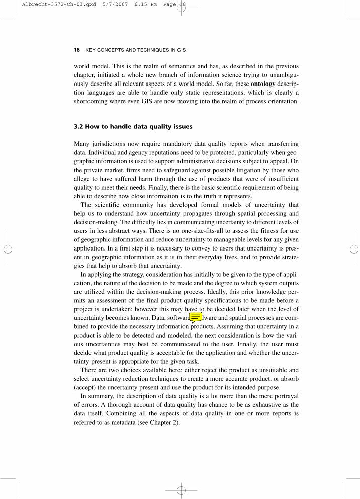
Many jurisdictions now require mandatory data quality reports when transferringdata. Individual and agency reputations need to be protected, particularly when geo-graphic information is used to support administrative decisions subject to appeal. Onthe private market, firms need to safeguard against possible litigation by those whoallege to have suffered harm through the use of products that were of insufficientquality to meet their needs. Finally, there is the basic scientific requirement of beingable to describe how close information is to the truth it represents.
The scientific community has developed formal models of uncertainty thathelp us to understand how uncertainty propagates through spatial processing anddecision-making. The difficulty lies in communicating uncertainty to different levels ofusers in less abstract ways. There is no one-size-fits-all to assess the fitness for useof geographic information and reduce uncertainty to manageable levels for any givenapplication. In a first step it is necessary to convey to users that uncertainty is pres-ent in geographic information as it is in their everyday lives, and to provide strate-gies that help to absorb that uncertainty.
In applying the strategy, consideration has initially to be given to the type of appli-cation, the nature of the decision to be made and the degree to which system outputsare utilized within the decision-making process. Ideally, this prior knowledge per-mits an assessment of the final product quality specifications to be made before aproject is undertaken; however this may have to be decided later when the level ofuncertainty becomes known. Data, software hardware and spatial processes are com-bined to provide the necessary information products. Assuming that uncertainty in aproduct is able to be detected and modeled, the next consideration is how the vari-ous uncertainties may best be communicated to the user. Finally, the user mustdecide what product quality is acceptable for the application and whether the uncer-tainty present is appropriate for the given task.
There are two choices available here: either reject the product as unsuitable andselect uncertainty reduction techniques to create a more accurate product, or absorb(accept) the uncertainty present and use the product for its intended purpose.
In summary, the description of data quality is a lot more than the mere portrayalof errors. A thorough account of data quality has chance to be as exhaustive as thedata itself. Combining all the aspects of data quality in one or more reports isreferred to as metadata (see Chapter 2).
Albrecht-3572-Ch-03.qxd 5/7/2007 6:15 PM Page 18

Among the most elementary database operations is the quest to find a data item in adatabase. Regular databases typically use an indexing scheme that works like alibrary catalog. We might search for an item alphabetically by author, by title or bysubject. A modern alternative to this are the indexes built by desktop or Internetsearch engines, which basically are very big lookup tables for data that is physicallydistributed all over the place.
Spatial search works somewhat differently from that. One reason is that a spatialcoordinate consists of two indices at the same time, x and y. This is like looking forauthor and title at the same time. The second reason is that most people, when theylook for a location, do not refer to it by its x/y coordinate. We therefore have to trans-late between a spatial reference and the way it is stored in a GIS database. Finally,we often describe the place that we are after indirectly, such as when looking for alldry cleaners within a city to check for the use of a certain chemical.
In the following, we will look at spatial queries starting with some very basicexamples and ending with rather complex queries that actually require some spatialanalysis before they can be answered. This chapter does deliberately omit anydiscussion of special indexing methods, which would be of interest to a computerscientist but perhaps not to the intended audience of this book.
4.1 Simple spatial querying
When we open a spatial dataset in a GIS, the default view on the data is to see it dis-played like a map (see Figure 8). Even the most basic systems then allow you to usea query tool to point to an individual feature and retrieve its attributes. They keyword here is ‘feature’; that is, we are looking at databases that actually store featuresrather than field data.
If the database is raster-based, then we have different options, depending on thesophistication of the system. Let’s have a more detailed look at the right part ofFigure 8. What is displayed here is an elevation dataset. The visual representationsuggests that we have contour lines but this does not necessarily mean that this is theway the data is actually stored and can hence be queried by. If it is indeed line data,then the current cursor position would give us nothing because there is no informa-tion stored for anything in between the lines. If the data is stored as areas (eachplateau of equal elevation forming one area), then we could move around betweenany two lines and would always get the same elevation value. Only once we cross aline would we ‘jump’ to the next higher or lower plateau. Finally, the data could be
4 SPATIAL SEARCH
Albrecht-3572-Ch-04.qxd 5/7/2007 6:39 PM Page 19

20 KEY CONCEPTS AND TECHNIQUES IN GIS
stored as a raster dataset, but rather than representing thousands of different eleva-tion values by as many colors, we may make life easier for the computer as well asfor us (interpreting the color values) by displaying similar elevation values with onlyone out of say 16 different color values. In this case, the hovering cursor could stillquery the underlying pixel and give us the more detailed information that we couldnot possibly distinguish by the hue.
This example illustrates another crucial aspect of GIS: the way we store data hasa major impact on what information can be retrieved. We will revisit this themerepeatedly throughout the book. Basically, data that is not stored, like the areabetween lines, cannot simply be queried. It would require rather sophisticated ana-lytical techniques to interpolate between the lines to come up with a guesstimate forthe elevation when the cursor is between the lines. If, on the other hand, the eleva-tion is explicitly stored for every location on the screen, then the spatial query isnothing but a simple lookup.
4.2 Conditional querying
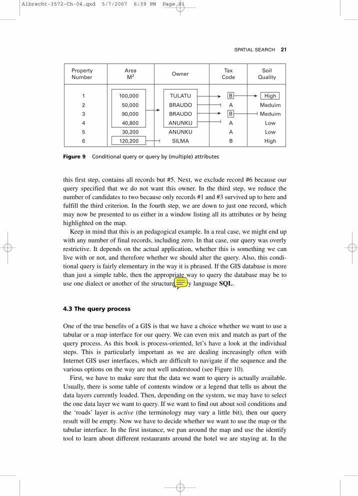
Conditional queries are just one notch up on the level of complication. Within a GIS,the condition can be either attribute- or geometry-based. To keep it simple and getthe idea across, let’s for now look at attributes only (see Figure 9).
Here, we have a typical excerpt from an attribute table with multiple variables. Aconditional query works like a filter that initially accesses the whole database.Similar to the way we search for a URL in an Internet search engine, we now pro-vide the system with all the criteria that have to be fulfilled for us to be interested inthe final presentation of records. Basically, what we are doing is to reject ever morerecords until we end up with a manageable number of them. In our case, we firstexclude record #5 because it does not fulfill the first criterion. Our selection set, after
Parcel# 231-12-687Owner John DoeZoning A3Value 179,820
Figure 8 Simple query by location
Albrecht-3572-Ch-04.qxd 5/7/2007 6:39 PM Page 20
SPATIAL SEARCH 21
this first step, contains all records but #5. Next, we exclude record #6 because ourquery specified that we do not want this owner. In the third step, we reduce thenumber of candidates to two because only records #1 and #3 survived up to here andfulfill the third criterion. In the fourth step, we are down to just one record, whichmay now be presented to us either in a window listing all its attributes or by beinghighlighted on the map.
Keep in mind that this is an pedagogical example. In a real case, we might end upwith any number of final records, including zero. In that case, our query was overlyrestrictive. It depends on the actual application, whether this is something we canlive with or not, and therefore whether we should alter the query. Also, this condi-tional query is fairly elementary in the way it is phrased. If the GIS database is morethan just a simple table, then the appropriate way to query the database may be touse one dialect or another of the structure query language SQL.
4.3 The query process
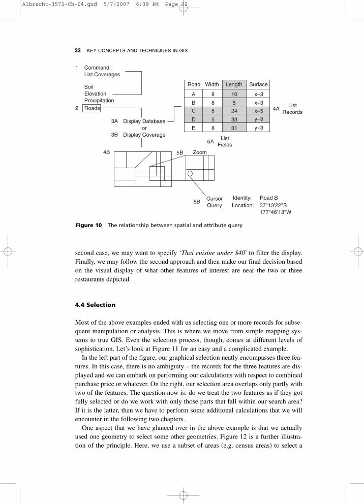
One of the true benefits of a GIS is that we have a choice whether we want to use atabular or a map interface for our query. We can even mix and match as part of thequery process. As this book is process-oriented, let’s have a look at the individualsteps. This is particularly important as we are dealing increasingly often withInternet GIS user interfaces, which are difficult to navigate if the sequence and thevarious options on the way are not well understood (see Figure 10).
First, we have to make sure that the data we want to query is actually available.Usually, there is some table of contents window or a legend that tells us about thedata layers currently loaded. Then, depending on the system, we may have to selectthe one data layer we want to query. If we want to find out about soil conditions andthe ‘roads’ layer is active (the terminology may vary a little bit), then our queryresult will be empty. Now we have to decide whether we want to use the map or thetabular interface. In the first instance, we pan around the map and use the identifytool to learn about different restaurants around the hotel we are staying at. In the
PropertyNumber
AreaM2 Owner
TaxCode
SoilQuality
1 100,000 TULATU High
High
B
BRAUDO MeduimA
BRAUDO MeduimB
ANUNKU Low
Low
A
ANUNKU A
SILMA B
50,0002
90,0003
40,8004
30,2005
120,2006
Figure 9 Conditional query or query by (multiple) attributes
Albrecht-3572-Ch-04.qxd 5/7/2007 6:39 PM Page 21
22 KEY CONCEPTS AND TECHNIQUES IN GIS
second case, we may want to specify ‘Thai cuisine under $40’ to filter the display.Finally, we may follow the second approach and then make our final decision basedon the visual display of what other features of interest are near the two or threerestaurants depicted.
4.4 Selection
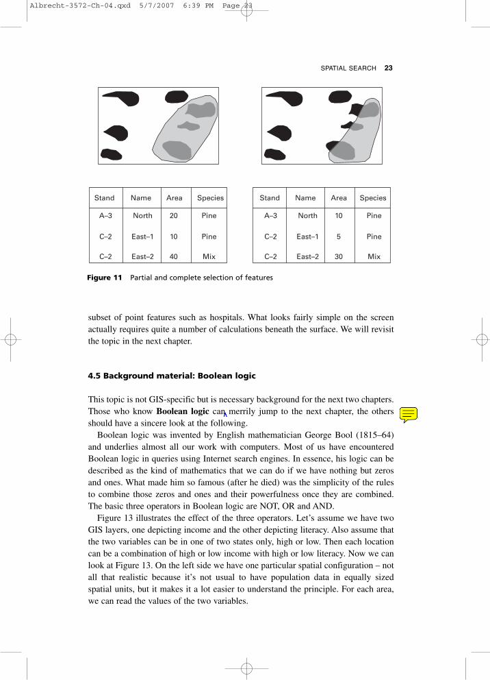
Most of the above examples ended with us selecting one or more records for subse-quent manipulation or analysis. This is where we move from simple mapping sys-tems to true GIS. Even the selection process, though, comes at different levels ofsophistication. Let’s look at Figure 11 for an easy and a complicated example.
In the left part of the figure, our graphical selection neatly encompasses three fea-tures. In this case, there is no ambiguity – the records for the three features are dis-played and we can embark on performing our calculations with respect to combinedpurchase price or whatever. On the right, our selection area overlaps only partly withtwo of the features. The question now is: do we treat the two features as if they gotfully selected or do we work with only those parts that fall within our search area?If it is the latter, then we have to perform some additional calculations that we willencounter in the following two chapters.
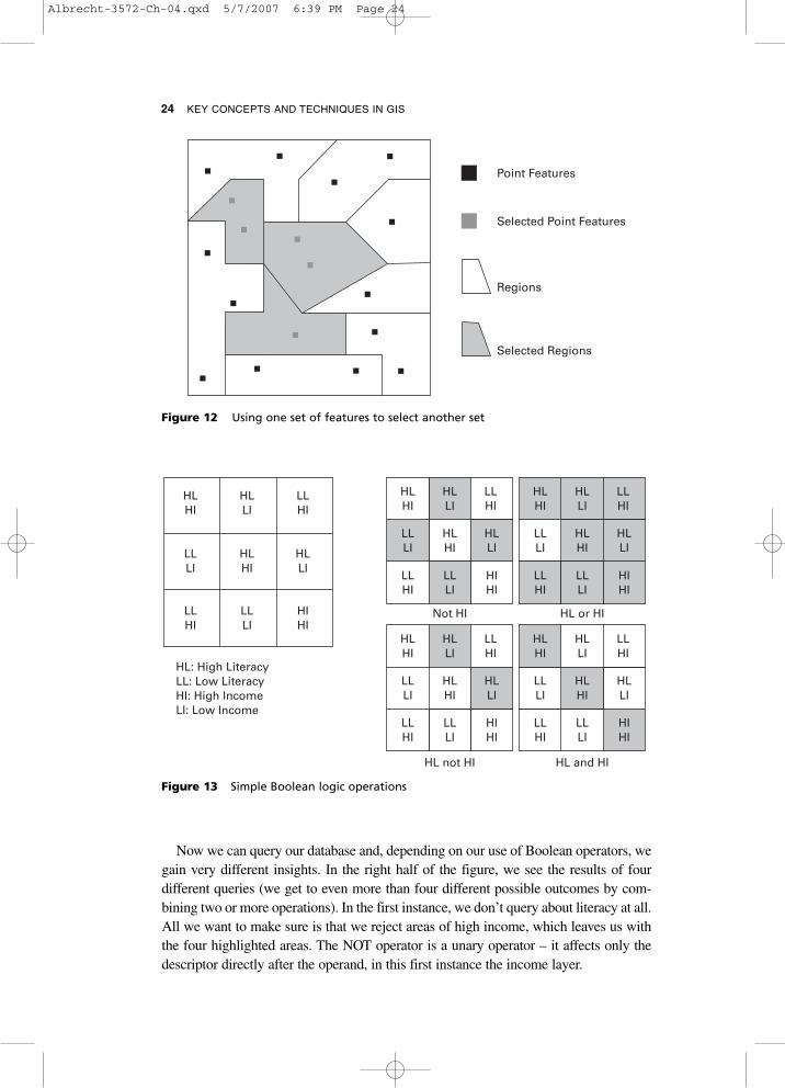
One aspect that we have glanced over in the above example is that we actuallyused one geometry to select some other geometries. Figure 12 is a further illustra-tion of the principle. Here, we use a subset of areas (e.g. census areas) to select a
Command:List Coverages
SoilElevationPrecipitationRoads
Road Width Length Surface
A
B
C
D
E
8
8
5
5
8
10
5
24
33
31
x–3
x–3
x–5
y–3
y–3
4A List
Records
ListFields
5A
5B
3A
3B
Display Databaseor
Display Coverage
4B
6B
Zoom
CursorQuery
Identity: Road BLocation: 37°13’22’’S
177°46’13’’W
1
2
Figure 10 The relationship between spatial and attribute query
Albrecht-3572-Ch-04.qxd 5/7/2007 6:39 PM Page 22
SPATIAL SEARCH 23
subset of point features such as hospitals. What looks fairly simple on the screenactually requires quite a number of calculations beneath the surface. We will revisitthe topic in the next chapter.
4.5 Background material: Boolean logic
This topic is not GIS-specific but is necessary background for the next two chapters.Those who know Boolean logic can merrily jump to the next chapter, the othersshould have a sincere look at the following.
Boolean logic was invented by English mathematician George Bool (1815–64)and underlies almost all our work with computers. Most of us have encounteredBoolean logic in queries using Internet search engines. In essence, his logic can bedescribed as the kind of mathematics that we can do if we have nothing but zerosand ones. What made him so famous (after he died) was the simplicity of the rulesto combine those zeros and ones and their powerfulness once they are combined.The basic three operators in Boolean logic are NOT, OR and AND.
Figure 13 illustrates the effect of the three operators. Let’s assume we have twoGIS layers, one depicting income and the other depicting literacy. Also assume thatthe two variables can be in one of two states only, high or low. Then each locationcan be a combination of high or low income with high or low literacy. Now we canlook at Figure 13. On the left side we have one particular spatial configuration – notall that realistic because it’s not usual to have population data in equally sizedspatial units, but it makes it a lot easier to understand the principle. For each area,we can read the values of the two variables.
Stand Name Area Species
A–3 North 20 Pine
Pine
Mix
10
40
East–1
East–2
C–2
C–2
Stand Name Area Species
A–3 North 10 Pine
Pine
Mix
5
30
East–1
East–2
C–2
C–2
Figure 11 Partial and complete selection of features
Albrecht-3572-Ch-04.qxd 5/7/2007 6:39 PM Page 23
24 KEY CONCEPTS AND TECHNIQUES IN GIS
Now we can query our database and, depending on our use of Boolean operators, wegain very different insights. In the right half of the figure, we see the results of fourdifferent queries (we get to even more than four different possible outcomes by com-bining two or more operations). In the first instance, we don’t query about literacy at all.All we want to make sure is that we reject areas of high income, which leaves us withthe four highlighted areas. The NOT operator is a unary operator – it affects only thedescriptor directly after the operand, in this first instance the income layer.
Point Features
Selected Point Features
Regions
Selected Regions
Figure 13 Simple Boolean logic operations
Figure 12 Using one set of features to select another set
HLHI
HLLI
LLHI
HLLI
HLHI
LLLI
LLHI
LLLI
HIHI
HLHI
HLLI
LLHI
HLLI
HLHI
LLLI
LLHI
LLLI
HIHI
HLHI
HLLI
LLHI
HLLI
HLHI
LLLI
LLHI
LLLI
HIHI
HLHI
HLLI
LLHI
HLLI
HLHI
LLLI
LLHI
LLLI
HIHI
HLHI
HLLI
LLHI
HLLI
HLHI
LLLI
LLHI
LLLI
HIHI
HL not HI
HL: High LiteracyLL: Low LiteracyHI: High IncomeLI: Low Income
HL and HI
HL or HINot HI
Albrecht-3572-Ch-04.qxd 5/7/2007 6:39 PM Page 24
Next, look at the OR operand. Translated into plain English, OR means ‘one orthe other, I don’t care which one’. This is in effect an easy-going operand, whereonly one of the two conditions needs to be fulfilled, and if both are true then thebetter. So, no matter whether we look at income or literacy, as long as either one (orboth) is high, the area gets selected. OR operations always result in a maximumnumber of items to be selected.
Somewhat contrary to the way the word is used in everyday English, AND doesnot give us the combination of two criteria but only those records that fulfill bothconditions. So in our case, only those areas that have both high literacy and highincome at the same time are selected. In effect, the AND operand acts like a strongfilter. We saw this above in the section on conditional queries, where all conditionshad to be fulfilled.
The last example illustrates that we can combine Boolean operations. Here welook for all areas that have a high literacy rate but not high income. It is a combina-tion of our first example (NOT HI) with the AND operand. The result becomes clearif we rearrange the query to state NOT HI AND HL. We say that AND and OR arebinary operands, which means they require one descriptor on the left and one on theright side. As in regular algebra, parentheses () can be used to specify the sequencein which the statement should be interpreted. If there are no parentheses, then NOTprecedes (overrides) the other two.
SPATIAL SEARCH 25
Albrecht-3572-Ch-04.qxd 5/7/2007 6:39 PM Page 25

Spatial relationships are one of the main reasons why one would want to use a GIS.Many of the cartographic characteristics of a GIS can be implemented with a draw-ing program, while the repository function of large spatial databases is often takencare of by traditional database management systems. It is the explicit storage ofspatial relationships and/or their analysis based on geometric reasoning that distin-guishes GIS from the rest of the pack.
We ended the last chapter with a select-by-location operation, which alreadymakes use of a derived relationship between areas and points that lay either insideor outside these areas. Before we embark on a discussion of many other importantspatial relationships, we should insert a little interlude in the form of the spatial data-base operation ‘recode’. Functionally, and from the perspective of typical GIS usage,this operation sits in between simple spatial queries and more advanced analyticalfunctions that result in new data.
5.1 Recoding
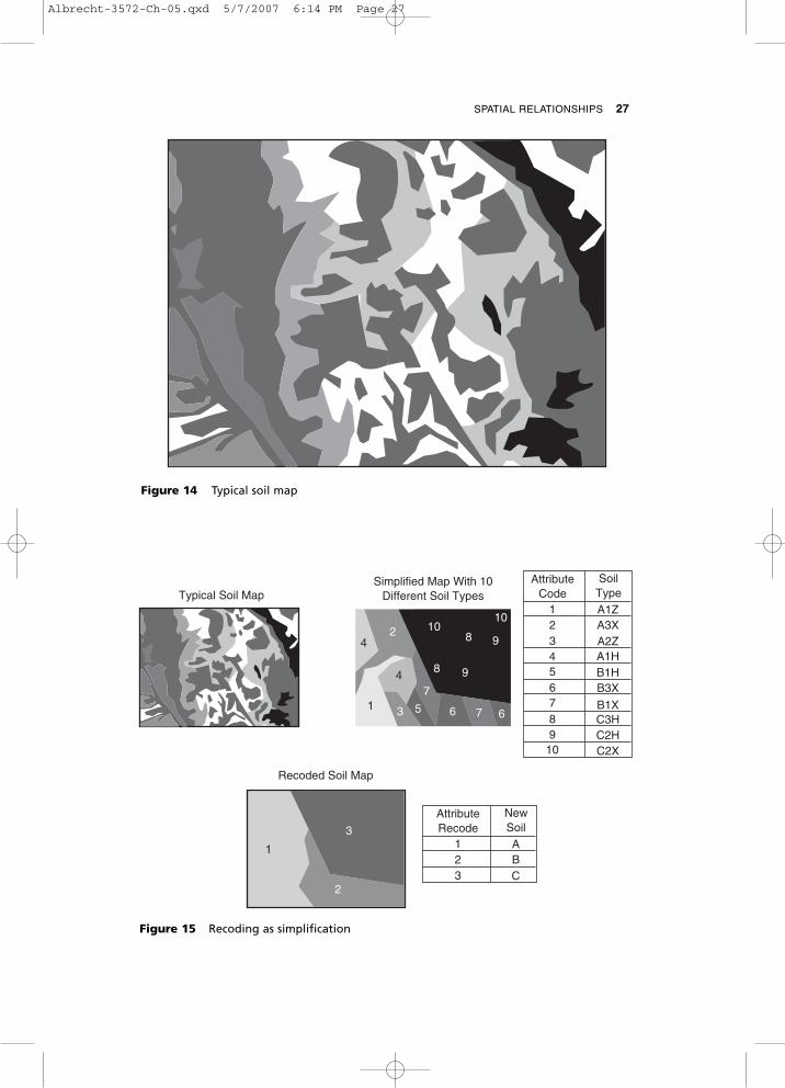
Recoding is an operation that is usually applied when the contents of a database havebecome confusingly complicated; as such it is used to simplify (our view of) thedatabase. Soil maps, such as the one depicted in Figure 14, are a perfect example ofthat. Ten different soil types may be of interest to the pedologist, but for most oth-ers it is sufficient to know whether the ground is stable enough to build a high-riseor dense enough to prevent groundwater leakages. In that case, we would like toaggregate the highly detailed information contained in a soils database and recodingis the way to do it.
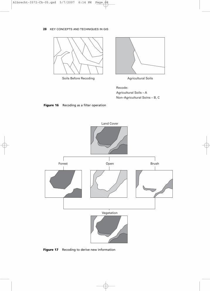
Figure 15 is a stylized version of the previous soil map and illustrates how thecombination of attributes also leads to a combination of geometries. We will makeuse of this side effect in the next chapter, when as a result of combining spatial data,we have more geometries than we would like. Alternatively, we could use the recod-ing operation not as much to simplify our view of the database but to reflect a par-ticular interpretation of the data. A simple application of this is given in Figure 16,where we simplify a complex map to a binary suitable/non-suitable for agriculturalpurposes.
A more complicated (and interesting) version of the same procedure is given inFigure 17. Here, we recode a complex landcover map by first extracting all differentvegetation types and then recombine these to form a new dataset containing all kindsof vegetation and nothing but vegetation. In both of these examples, we are creating
5 SPATIAL RELATIONSHIPS
Albrecht-3572-Ch-05.qxd 5/7/2007 6:14 PM Page 26
SPATIAL RELATIONSHIPS 27
Figure 14 Typical soil map
Typical Soil Map
Recoded Soil Map
Simplified Map With 10Different Soil Types
AttributeCode
SoilType
4
4
1 3
2 1010
9
66
7
5 7
98
8
1 A1ZA3XA2ZA1HB1HB3X
B1XC3HC2HC2X
23456789
10
AttributeRecode
NewSoil
11 ABC
23
2
3
Figure 15 Recoding as simplification
Albrecht-3572-Ch-05.qxd 5/7/2007 6:14 PM Page 27
28 KEY CONCEPTS AND TECHNIQUES IN GIS
Soils Before Recoding
Agricultural Soils – A
Agricultural Soils
Non–Agricultural Soins – B, C
Recode:
Figure 16 Recoding as a filter operation
Land Cover
Open BrushForest
Vegetation
Figure 17 Recoding to derive new information
Albrecht-3572-Ch-05.qxd 5/7/2007 6:14 PM Page 28
new data based on a new interpretation of already existing data. There is no category‘vegetation’ in the original landcover dataset. We will revisit the topic of creating newdata rather than just querying existing data in the next chapter on combining data. Thissneak preview is an indicator of the split personality of the recoding operation; it couldbe interpreted as a mere data maintenance operation or as an analytical one.
One intriguing aspect that comes to mind when one looks at Figures 16 and 17 isthat we immediately try to discern patterns in the distribution of selected areas.Spatial relationships can be studied quantitatively or qualitatively. The former willbe the subject of Chapter 10, while the latter is addressed in the following sections.Features are defined by their boundaries. On the qualitative side, we can thereforedistinguish between two types of spatial relationship, one where we look at howindividual coordinates are combined to form feature boundaries and the other wherewe look at the spatial relationships among features.
5.2 Relationships between measurements
As discussed in Chapter 2, all locational references can be reduced to one or morecoordinates, which are either measured or interpolated. It is important to remind our-selves that we are talking about the data in our geographic databases, not the geome-tries that are used to visualize the geographic data, which may be the same but mostlikely are not. If you are unsure about this topic, please revisit Chapter 2.
Next, we need to distinguish between the object-centered and the field-based rep-resentations of geographic information (see also Chapter 1). The latter does not haveany feature representation, so the spatial relationships are reduced to those of therespective positions of pixels to each other. This then is very straightforward, as wehave only a very limited number of scenarios, as depicted in Figure 18:
• Cell boundaries can touch each other.• Cell corners can touch each other.• Cells don’t touch each other at all.• Cells relate to each other not within a layer but across (vertically).
We will revisit the cell relationships in Chapter 8, when we look at the analyticalcapabilities of raster GIS – which are entirely based on the simplicity of their spatialrelationships.
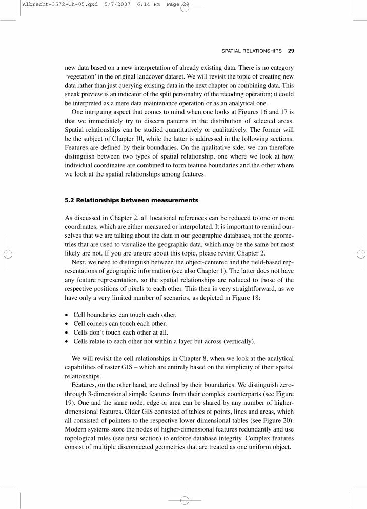
Features, on the other hand, are defined by their boundaries. We distinguish zero-through 3-dimensional simple features from their complex counterparts (see Figure19). One and the same node, edge or area can be shared by any number of higher-dimensional features. Older GIS consisted of tables of points, lines and areas, whichall consisted of pointers to the respective lower-dimensional tables (see Figure 20).Modern systems store the nodes of higher-dimensional features redundantly and usetopological rules (see next section) to enforce database integrity. Complex featuresconsist of multiple disconnected geometries that are treated as one uniform object.
SPATIAL RELATIONSHIPS 29
Albrecht-3572-Ch-05.qxd 5/7/2007 6:14 PM Page 29

30 KEY CONCEPTS AND TECHNIQUES IN GIS
No TouchingAt All
No Relationship within,but Across Layers
Corners TouchEach other
Boundries TouchEach other
Figure 18 Four possible spatial relationships in a pixel world
Figure 19 Simple (top row) and complex (bottom row) geometries
Albrecht-3572-Ch-05.qxd 5/7/2007 6:14 PM Page 30
SPATIAL RELATIONSHIPS 31
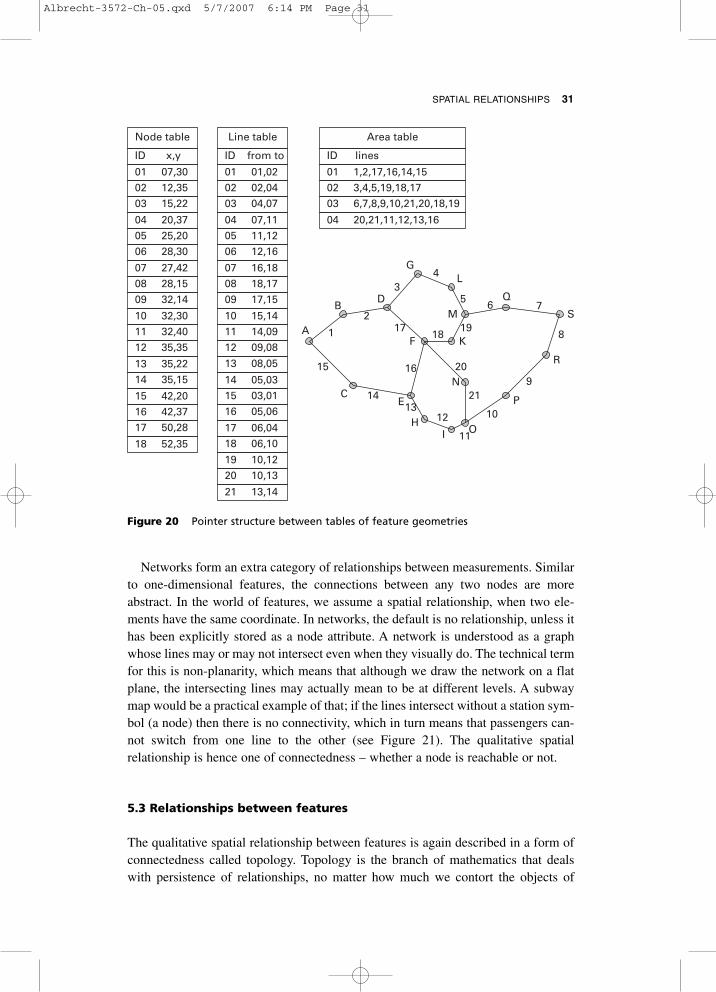
Networks form an extra category of relationships between measurements. Similarto one-dimensional features, the connections between any two nodes are moreabstract. In the world of features, we assume a spatial relationship, when two ele-ments have the same coordinate. In networks, the default is no relationship, unless ithas been explicitly stored as a node attribute. A network is understood as a graphwhose lines may or may not intersect even when they visually do. The technical termfor this is non-planarity, which means that although we draw the network on a flatplane, the intersecting lines may actually mean to be at different levels. A subwaymap would be a practical example of that; if the lines intersect without a station sym-bol (a node) then there is no connectivity, which in turn means that passengers can-not switch from one line to the other (see Figure 21). The qualitative spatialrelationship is hence one of connectedness – whether a node is reachable or not.
5.3 Relationships between features
The qualitative spatial relationship between features is again described in a form ofconnectedness called topology. Topology is the branch of mathematics that dealswith persistence of relationships, no matter how much we contort the objects of
Node table Line table Area table
01 07,3002 12,3503 15,22
04 20,3705 25,2006 28,30
01 01,0202 02,0403 04,07
04 07,1105 11,1206 12,16
01 1,2,17,16,14,1502 3,4,5,19,18,1703 6,7,8,9,10,21,20,18,19
04 20,21,11,12,13,16
ID x,y ID from to ID lines
07 16,1808 18,1709 17,15
10 15,1411 14,0912 09,08
13 08,05
14 05,0315 03,0116 05,06
17 06,0418 06,10
19 10,1220 10,13
21 13,14
07 27,4208 28,1509 32,14
10 32,3011 32,4012 35,35
13 35,2214 35,15
15 42,2016 42,3717 50,28
18 52,35
1
2
34
5 6 7
8
9
10
11
1213
14
15 16
1718A
B
C
D
E
F
G
HI
K
L
M
N
19
20
21
O
P
R
S
Q
Figure 20 Pointer structure between tables of feature geometries
Albrecht-3572-Ch-05.qxd 5/7/2007 6:14 PM Page 31
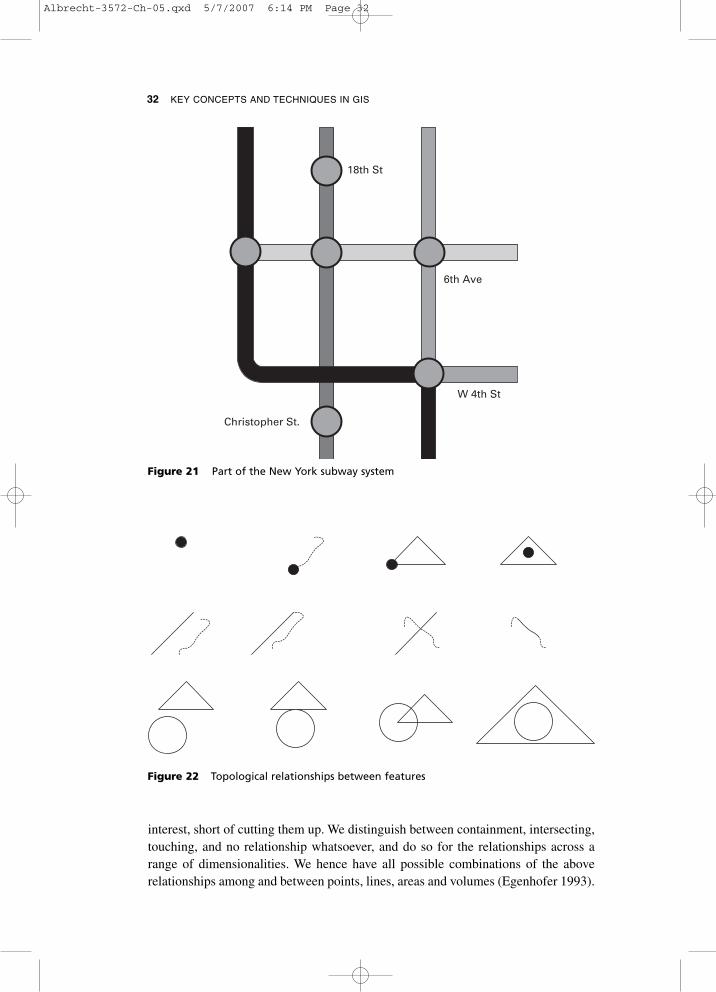
32 KEY CONCEPTS AND TECHNIQUES IN GIS
interest, short of cutting them up. We distinguish between containment, intersecting,touching, and no relationship whatsoever, and do so for the relationships across arange of dimensionalities. We hence have all possible combinations of the aboverelationships among and between points, lines, areas and volumes (Egenhofer 1993).
18th St
6th Ave
W 4th St
Christopher St.
Figure 21 Part of the New York subway system
Figure 22 Topological relationships between features
Albrecht-3572-Ch-05.qxd 5/7/2007 6:14 PM Page 32
SPATIAL RELATIONSHIPS 33
Figure 22 lists a selection of such topological relationships. Volumes have beenwritten about what are the mathematically distinguishable qualitative relationships,how they relate to quantitative measures, and whether we even have names for themin different human languages. In English, for instance, we use verbs such as touch,border, intersect, overlap and contain, to describe the relationships depicted inFigure 22.
The use of topological rules has proven to be a very useful instrument for check-ing the consistency of a GIS database. Until recently, GIS could store only one typeof geometry per feature class. Spatial relationships within one and the same featureclass can be encoded as part of the data structure, which imposes additional con-straints on the data organization and helps to check for database consistency. If theserules are applied across feature classes, then we have to (a) perform a topology checkby at least temporarily combining spatial features, and (b) store these in an extratable that is associated with a group of feature classes. We will revisit this topic inthe next chapter about combining spatial data.
Albrecht-3572-Ch-05.qxd 5/7/2007 6:14 PM Page 33

As mentioned in the previous chapter, many spatial relationships are difficult toderive or even describe. Rather than storing all possible relationships between allfeatures of a database, we rather use GIS operations to answer specific questionsabout the spatial relationships among our features of interest. This is not only farmore efficient but also gives us more freedom, because we can determine on the flywhat pieces of data we want to relate to each other – and in the age of the Internet,these pieces may even be distributed across the world.
This chapter deals with two families of GIS operations that in practice make upsome 75–80% of all analytical GIS operations. Overlay is the quintessential GISoperation that seems to define a GIS. If a software package can perform overlayoperations, then it is indeed a GIS and not a mere CAD or cartography program. Thepoor cousin is the buffer operation, which always seems to be mentioned second.Both are actually place-holders for a number of different operations, but we willdiscuss this in detail in the following.
6.1 Overlay
In the recoding section of the last chapter, we saw how tightly linked attributes andgeometries are. By recombining attributes we automatically changed the graphicalrepresentation as well. However, when we look at it from the perspective of linesstore in our database (see Figure 20), the recoding operation did not create any newgeometries. This changes now with the group of overlay operations. Let’s look atFigure 23 to see what happens to geometries and attributes in an overlay operation.
For pedagogical reasons, we use very simple geometries and only two layers ofbinary data. This is extremely unrealistic but helps us to get the principle across. Wewill look at more realistic examples later on.
The figure shows a number of important aspects of the overlay operation. We havetwo or more input feature classes and one (new) output feature class. The geometriesof the two input layers are most likely to be different; that is, they do not have tocome from the same provider and do not have to have anything in common otherthan the general extent (it does not make sense to overlay data in South America withother data from Africa). Also observe that the first feature class has no attributesdescribing vegetation, while the second has none describing soils. The overlay oper-ation depicted here looks for coincidences at the same location. In other words, forany given location, it looks what information there is in one feature class, then in the
6 COMBINING SPATIAL DATA
Albrecht-3572-Ch-06.qxd 5/7/2007 6:12 PM Page 34

COMBINING SPATIAL DATA 35
other feature class, and then it combines the two in the output dataset. The geome-tries of the output dataset did not exist before. We really create completely new data.
We used this notion of coincidence earlier when we looked at some of the moreadvanced spatial search functions. Figure 24 is a case in point.
InputFeature Class 1
InputFeature Class 1
OutputFeature Class 3
+
=
Polygon Type Size
Polygon Type Size
Polygon Type Size
1 Clay 2Sand 22
A
1A 1111
Clay GrassSand Grass
Sand TreesClay Trees
2A1B2B
Grass 22TreesB
Soils
Vegitation
CLAY
1 2SAND
GRASS
2A1A
2B1B
TREES
A
B
Figure 23 Schematics of a polygon overlay operation
Soils
Which Soils Occure in County C?
Coincidence View
Counties
AB
C
D E
Figure 24 Overlay as a coincidence function
Albrecht-3572-Ch-06.qxd 5/7/2007 6:12 PM Page 35
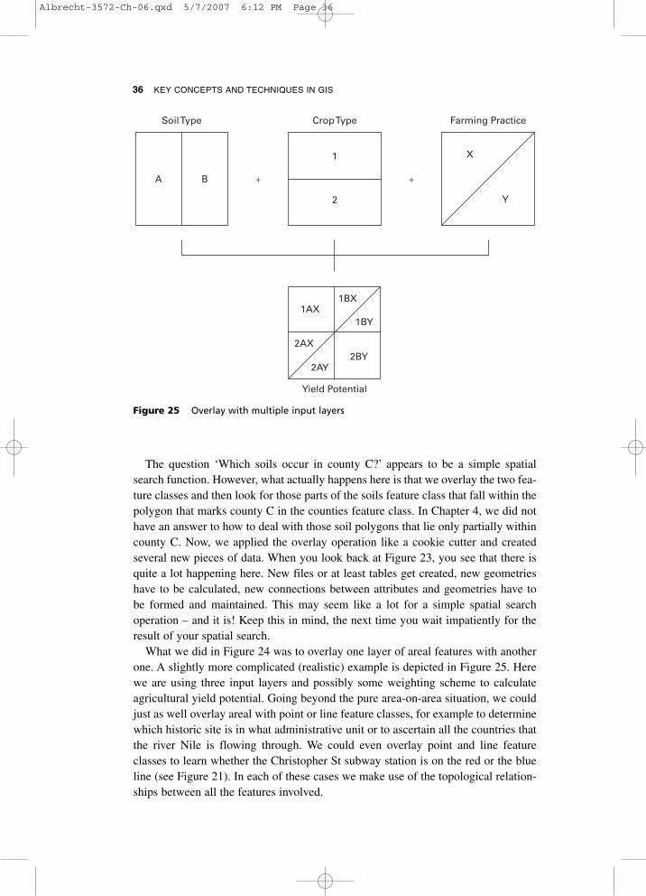
36 KEY CONCEPTS AND TECHNIQUES IN GIS
The question ‘Which soils occur in county C?’ appears to be a simple spatialsearch function. However, what actually happens here is that we overlay the two fea-ture classes and then look for those parts of the soils feature class that fall within thepolygon that marks county C in the counties feature class. In Chapter 4, we did nothave an answer to how to deal with those soil polygons that lie only partially withincounty C. Now, we applied the overlay operation like a cookie cutter and createdseveral new pieces of data. When you look back at Figure 23, you see that there isquite a lot happening here. New files or at least tables get created, new geometrieshave to be calculated, new connections between attributes and geometries have tobe formed and maintained. This may seem like a lot for a simple spatial searchoperation – and it is! Keep this in mind, the next time you wait impatiently for theresult of your spatial search.
What we did in Figure 24 was to overlay one layer of areal features with anotherone. A slightly more complicated (realistic) example is depicted in Figure 25. Herewe are using three input layers and possibly some weighting scheme to calculateagricultural yield potential. Going beyond the pure area-on-area situation, we couldjust as well overlay areal with point or line feature classes, for example to determinewhich historic site is in what administrative unit or to ascertain all the countries thatthe river Nile is flowing through. We could even overlay point and line featureclasses to learn whether the Christopher St subway station is on the red or the blueline (see Figure 21). In each of these cases we make use of the topological relation-ships between all the features involved.
Soil Type Crop Type
Yield Potential
1AX1BX
1BY
2BY2AY
2AX
Farming Practice
A B
1
2 Y
X
+ +
Figure 25 Overlay with multiple input layers
Albrecht-3572-Ch-06.qxd 5/7/2007 6:12 PM Page 36
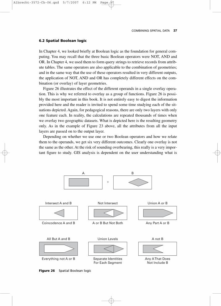
COMBINING SPATIAL DATA 37
6.2 Spatial Boolean logic
In Chapter 4, we looked briefly at Boolean logic as the foundation for general com-puting. You may recall that the three basic Boolean operators were NOT, AND andOR. In Chapter 4, we used them to form query strings to retrieve records from attrib-ute tables. The same operators are also applicable to the combination of geometries;and in the same way that the use of these operators resulted in very different outputs,the application of NOT, AND and OR has completely different effects on the com-bination (or overlay) of layer geometries.
Figure 26 illustrates the effect of the different operands in a single overlay opera-tion. This is why we referred to overlay as a group of functions. Figure 26 is possi-bly the most important in this book. It is not entirely easy to digest the informationprovided here and the reader is invited to spend some time studying each of the sit-uations depicted. Again, for pedagogical reasons, there are only two layers with onlyone feature each. In reality, the calculations are repeated thousands of times whenwe overlay two geographic datasets. What is depicted here is the resulting geometryonly. As in the example of Figure 23 above, all the attributes from all the inputlayers are passed on to the output layer.
Depending on whether we use one or two Boolean operators and how we relatethem to the operands, we get six very different outcomes. Clearly one overlay is notthe same as the other. At the risk of sounding overbearing, this really is a very impor-tant figure to study. GIS analysis is dependent on the user understanding what is
All But A and B
Everything not A or B Separate IdentitiesFor Each Segment
Any A That DoesNot Include B
Union Levels A not B
Intersect A and B
Coincodence A and B A or B But Not Both Any Part A or B
Not Intersect Union A or B
A
+
B
Figure 26 Spatial Boolean logic
Albrecht-3572-Ch-06.qxd 5/7/2007 6:12 PM Page 37
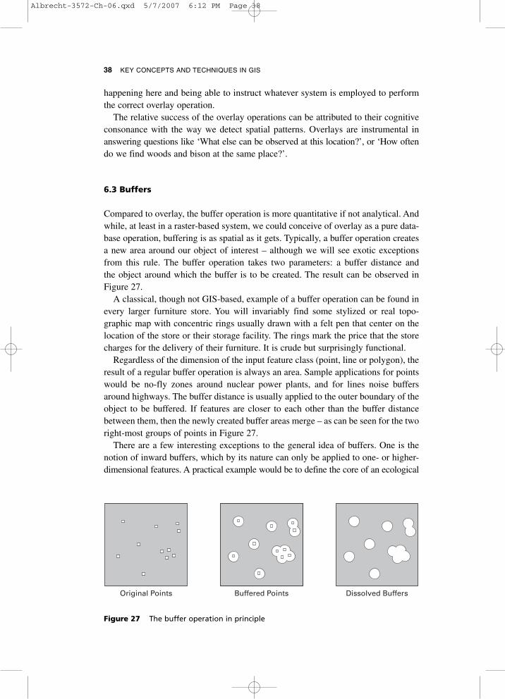
38 KEY CONCEPTS AND TECHNIQUES IN GIS
happening here and being able to instruct whatever system is employed to performthe correct overlay operation.
The relative success of the overlay operations can be attributed to their cognitiveconsonance with the way we detect spatial patterns. Overlays are instrumental inanswering questions like ‘What else can be observed at this location?’, or ‘How oftendo we find woods and bison at the same place?’.
6.3 Buffers
Compared to overlay, the buffer operation is more quantitative if not analytical. Andwhile, at least in a raster-based system, we could conceive of overlay as a pure data-base operation, buffering is as spatial as it gets. Typically, a buffer operation createsa new area around our object of interest – although we will see exotic exceptionsfrom this rule. The buffer operation takes two parameters: a buffer distance andthe object around which the buffer is to be created. The result can be observed inFigure 27.
A classical, though not GIS-based, example of a buffer operation can be found inevery larger furniture store. You will invariably find some stylized or real topo-graphic map with concentric rings usually drawn with a felt pen that center on thelocation of the store or their storage facility. The rings mark the price that the storecharges for the delivery of their furniture. It is crude but surprisingly functional.
Regardless of the dimension of the input feature class (point, line or polygon), theresult of a regular buffer operation is always an area. Sample applications for pointswould be no-fly zones around nuclear power plants, and for lines noise buffersaround highways. The buffer distance is usually applied to the outer boundary of theobject to be buffered. If features are closer to each other than the buffer distancebetween them, then the newly created buffer areas merge – as can be seen for the tworight-most groups of points in Figure 27.
There are a few interesting exceptions to the general idea of buffers. One is thenotion of inward buffers, which by its nature can only be applied to one- or higher-dimensional features. A practical example would be to define the core of an ecological
Original Points Buffered Points Dissolved Buffers
Figure 27 The buffer operation in principle
Albrecht-3572-Ch-06.qxd 5/7/2007 6:12 PM Page 38
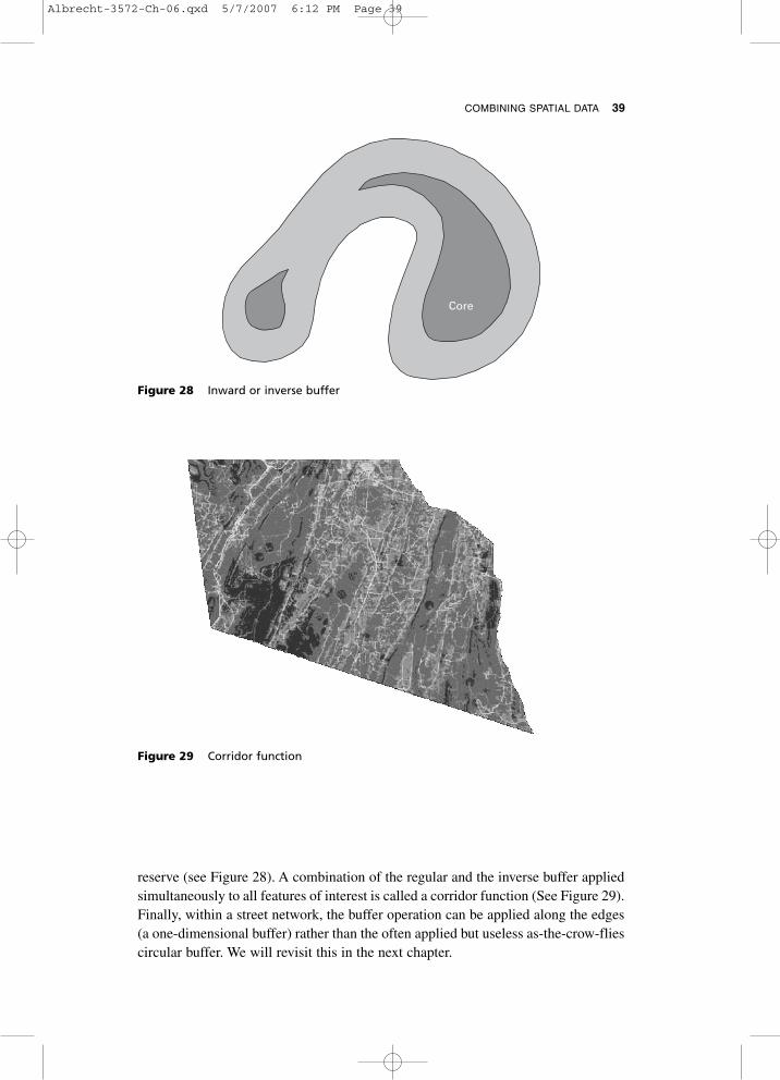
COMBINING SPATIAL DATA 39
reserve (see Figure 28). A combination of the regular and the inverse buffer appliedsimultaneously to all features of interest is called a corridor function (See Figure 29).Finally, within a street network, the buffer operation can be applied along the edges(a one-dimensional buffer) rather than the often applied but useless as-the-crow-fliescircular buffer. We will revisit this in the next chapter.
Core
Figure 28 Inward or inverse buffer
Figure 29 Corridor function
Albrecht-3572-Ch-06.qxd 5/7/2007 6:12 PM Page 39

40 KEY CONCEPTS AND TECHNIQUES IN GIS
6.4 Buffering in spatial search
A few paragraphs above, we saw how overlay underlies some of the (not overtly)more complicated spatial search operations. The same holds true for buffering.Conceptually, buffers are in this case used as a form of neighborhood. ‘Find allcustomers within ZIP code 123’ is an overlay operation, but ‘Find all customers in aradius of 5 miles’ is a buffer operation. Buffers are often used as an intermediateselect, where we use the result of the buffer operation in subsequent analysis (seenext section).
6.5 Combining operations
If the above statement that buffers and overlays make up in practice some 75% of allanalytical GIS functionality is true, then how is it that GIS has become such animportant genre of software? The solution to this paradox lies in the fact that opera-tions can be concatenated to form workflows. The following is an example from amajor flood in Mozambique in 2000 (see Figure 30).
Input Layers
Roads Towns River
Directly Affected;Under Water
Indirectly Affected;Dry but cut off
Not Affected at all
Overlay and Buffer
Overlay
Identification ofIndirectly AffectedTowns
Figure 30 Surprise effects of buffering affecting towns outside a flood zone
Albrecht-3572-Ch-06.qxd 5/7/2007 6:12 PM Page 40
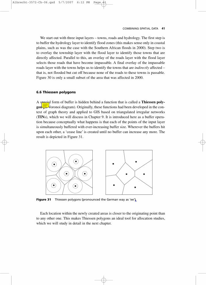
COMBINING SPATIAL DATA 41
We start out with three input layers – towns, roads and hydrology. The first step isto buffer the hydrology layer to identify flood zones (this makes sense only in coastalplains, such as was the case with the Southern African floods in 2000). Step two isto overlay the township layer with the flood layer to identify those towns that aredirectly affected. Parallel to this, an overlay of the roads layer with the flood layerselects those roads that have become impassable. A final overlay of the impassableroads layer with the towns helps us to identify the towns that are indirectly affected –that is, not flooded but cut off because none of the roads to these towns is passable.Figure 30 is only a small subset of the area that was affected in 2000.
6.6 Thiessen polygons
A special form of buffer is hidden behind a function that is called a Thiessen poly-gon (or Voronoi diagram). Originally, these functions had been developed in the con-text of graph theory and applied to GIS based on triangulated irregular networks(TINs), which we will discuss in Chapter 9. It is introduced here as a buffer opera-tion because conceptually what happens is that each of the points of the input layeris simultaneously buffered with ever-increasing buffer size. Wherever the buffers hitupon each other, a ‘cease line’ is created until no buffer can increase any more. Theresult is depicted in Figure 31.
Figure 31 Thiessen polygons (pronounced the German way as ‘ee’)
Each location within the newly created areas is closer to the originating point thanto any other one. This makes Thiessen polygons an ideal tool for allocation studies,which we will study in detail in the next chapter.
Albrecht-3572-Ch-06.qxd 5/7/2007 6:12 PM Page 41
Among the main reasons for wanting to use a GIS are (1) finding a location, (2) findingthe best way to get to that location, (3) finding the best location to do whatever ourbusiness is, and (4) optimizing the use of our limited resources to conduct ourbusiness. The first question has been answered at varying levels of complexity in theearlier chapters. Now I want to address the other three questions.
General GIS textbooks usually direct the reader to answer these questions byusing the third and so far neglected form of GIS data structure, the network GIS.This is, however, slightly misleading as we could just as well use map algebra(Chapter 8), and some of the more advanced regional science models would even usedata aggregated to polygons (although here the shape of the polygons and hencemuch of the reason why we would use vector GIS is not considered). The followingnotes are more about concepts; the actual procedures in raster or in network GISwould differ considerably from each other. But that is an implementation issue andshould not be of immediate concern to the end user.
7.1 The best way
Finding the best way to a particular location is usually referred to as shortest-pathanalysis. But that is shorthand for a larger group of operations, which we will lookat here. To determine the best way one needs at a minimum an origin and a destina-tion. On a featureless flat plain, the direct line between these two locations wouldmark the best way. In the real world, though, we have geography interfering with thissimple geometric view. Even if we limit ourselves to just the shortest distance, wetend to stay on streets (where available), don’t walk through walls, and don’t wantto get stuck in a traffic jam. Often, we have other criteria but pure distance that deter-mine which route we choose: familiarity, scenery, opportunity to get some otherbusiness done on the way, and so on. Finally, we typically are not the only ones toembark on a journey, say from home to work. Our decisions, our choice of what isthe best way, are influenced by what other people are doing, and they are time-dependent. An optimal route in the morning may not easily be traced back in theevening. In most general terms, what we are trying to accomplish with our best-wayanalysis is to model the flows of commodities, people, capital or information overspace (Reggiani 2001). How, then, can all these issues be addressed in a GIS, andhow does all this get implemented?
A beginning is to describe the origin and the target. This could be done in the formof two coordinate pairs, or a relative position given by distance and direction from
7 LOCATION–ALLOCATION
Albrecht-3572-Ch-07.qxd 5/7/2007 6:28 PM Page 42

LOCATION–ALLOCATION 43
an origin. Either location can be imbued with resources in the widest sense, possiblybetter described as push and pull factors. Assuming for a moment that the origin isa point (node, centroid, pixel), we can run a wide range of calculations on the attrib-utes of that point to determine what factors make the target more desirable than ourorigin and what resources to use to get there. The same is true for any point inbetween that we might visit or want to avoid. Finally, we have to decide how wewant to travel. There may be a constraining geometry underlying our geography. Inthe field view perspective we could investigate all locations within our view shed,whereas in a network we would be constrained by the links between the nodes.These links usually have a set of attributes of their own, determining speed, capac-ity (remember, we are unlikely to be the only ones with the wish to travel), or modeof transport. In a raster GIS, the attributes for links and nodes are combined at eachpixel, which actually makes it easier to deal with hybrid functionality such as turns.Turn tables are a special class of attribute table that permit or prevent us from chang-ing direction; they can also be used to switch modes of transportation. Each pixel,node or link could have its own schedule or a link to a big central time table thatdetermines the local behavior at any given time in the modeling scenario.
The task is then to determine the best way among all the options outlined above.Two coordinate pairs and a straight line between them rarely describes our real worldproblem adequately (we would not need a GIS for that). The full implementation ofall of the above options is as of writing this book just being tested for a few mid-sized cities. Just to assemble all the data (before even embarking on developing therouting algorithms) is a major challenge. Given the large number of options, we arefaced with an optimization problem. The implementation is usually based on graphtheoretical constructs (forward star search, Dijkstra algorithm) and will not be cov-ered here. But conceptually, the relationship between origins and targets is based onthe gravity model, which we will look at in the following section.
7.2 Gravity model
In the above section, we referred to the resources that we have available and talkedabout the push and pull of every point. This vocabulary is borrowed from a naivemodel of physics going all the way back to Isaac Newton. Locations influence eachother in a similar way that planets do in a solar system. Each variable exerts a fieldof influence around its center and that field is modeled using the same equations thatwere employed in mechanics. This intellectual source has provided lots of ammuni-tion for social scientists who thought the analogy to be too crude. But modern appli-cations of the gravity model in location–allocation models are as similar to Newton’srole model as a GPS receiver to a compass.
The gravity model in spatial analysis is the inductive formalization of Tobler’sFirst Law (see Chapter 10). Mathematically, we refer to a distance-decay function,which in Newton’s case was one over the square of distance but in spatial analysiscan be a wide range of functions. By way of example, $2 may get me 50 km away
Albrecht-3572-Ch-07.qxd 5/7/2007 6:28 PM Page 43

44 KEY CONCEPTS AND TECHNIQUES IN GIS
from the central station in New York, 20 km in Hamburg, Germany, and nowhere inDetroit if my mode of transport is a subway train. We can now associate fields ofinfluence based on a number of different metrics with each location in our dataset(see Figure 32). Sometimes they act as a resource as in our fare example, sometimesthey act as an attractor that determines how far we are willing to access a certainresource (school, hospital, etc.). Sometimes they may even act as a distracter, an areathat we don’t want to get too close to (nuclear power plants, prisons, predators).
North Carolina
Rocky Mount
Fayetteville
Wilmington
Statesville
Florence
South Carolina
SinksSources
Figure 32 Areas of influence determining the reach of gravitational pull
This push and pull across all known locations of a study area forms the basis foranswering the next question, finding the optimal location or site for a particularresource, be it a new fire station or a coffee shop. The next section will describe theconcepts behind location modeling.
7.3 Location modeling
Finding an optimal location has been the goal of much research in business schoolsand can be traced all the way back to nineteenth and early twentieth century schol-ars such as von Thünen, Weber and Christaller. The idea of the gravity model appliesto all of them (see Figures 33–35), albeit in increasingly complicated ways. VonThünen worked on an isolated agricultural town. Weber postulated a simple triangleof resource, manufacturer and market location. Christaller expanded this view into awhole network of spheres of influence.
Albrecht-3572-Ch-07.qxd 5/7/2007 6:28 PM Page 44
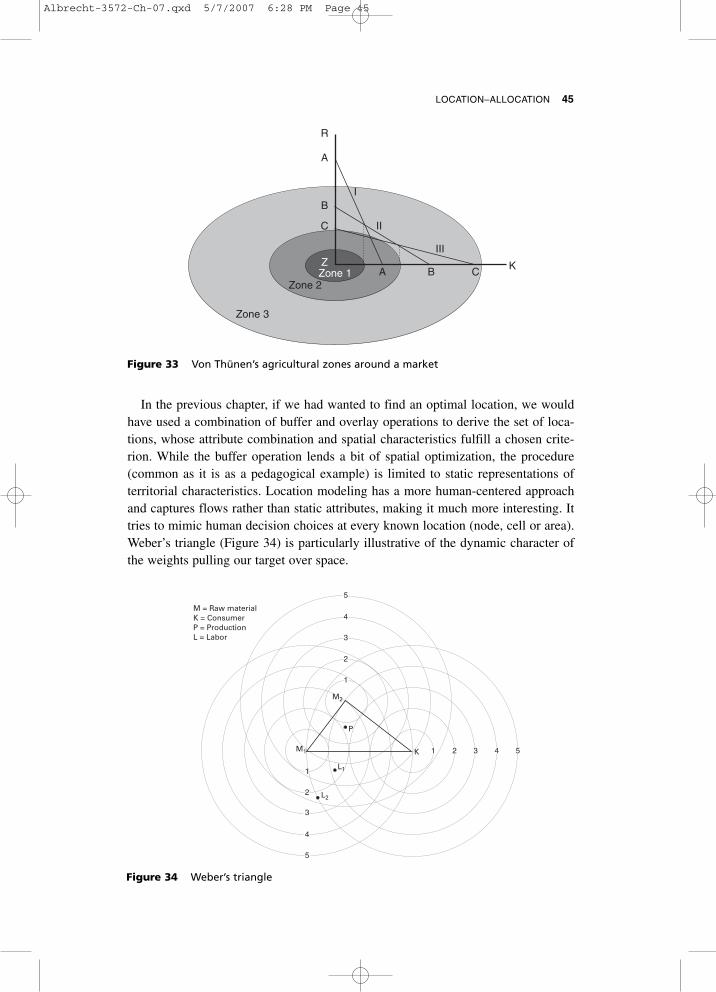
LOCATION–ALLOCATION 45
In the previous chapter, if we had wanted to find an optimal location, we wouldhave used a combination of buffer and overlay operations to derive the set of loca-tions, whose attribute combination and spatial characteristics fulfill a chosen crite-rion. While the buffer operation lends a bit of spatial optimization, the procedure(common as it is as a pedagogical example) is limited to static representations ofterritorial characteristics. Location modeling has a more human-centered approachand captures flows rather than static attributes, making it much more interesting. Ittries to mimic human decision choices at every known location (node, cell or area).Weber’s triangle (Figure 34) is particularly illustrative of the dynamic character ofthe weights pulling our target over space.
R
A
B
C
A B CKZ
I
II
III
Zone 1Zone 2
Zone 3
Figure 33 Von Thünen’s agricultural zones around a market
M = Raw materialK = ConsumerP = ProductionL = Labor
M2
M1
L1
L2
P
K 1 2 3 4 5
5
4
3
2
1
1
2
3
4
5
Figure 34 Weber’s triangle
Albrecht-3572-Ch-07.qxd 5/7/2007 6:28 PM Page 45

46 KEY CONCEPTS AND TECHNIQUES IN GIS
Two additions to this image drive the analogy home. Rather than having a planesurface, we model the weights pulling our optimal center across some rugged terrain.Each hill and peak marks push factors or locations we want to avoid. The number ofweights is equivalent to the number of locations that we assume to have an influenceover our optimal target site. The weights themselves finally consist of as manycriteria given as much weight as we wish to apply. The weights could even varydepending on time of day, or season, or real-time sensor readings. The latter wouldthen be an example for the placement of sentinels in a public safety scenario.
Central PlaceTheory
Boundaries
Village
Town
City
Figure 35 Christaller’s Central Place theory
The implementation of such a system of gravity models is fairly straightforwardfor a raster model (as we will see in the discussion of zonal operations in the fol-lowing chapter) or a network model (particularly if our commodities are shippedalong given routes). For a system of regions interacting with each other, the imple-mentation is traditionally less feature-based. Instead, large input–output tablesrepresenting the flows from each area to each other area are used in what is called aflow matrix (see Figure 36). The geometry of each of these areas is neglected andthe flows are aggregated to one in each direction across a boundary. Traditionallyemployed in regional science applications, the complications of geometry are
Albrecht-3572-Ch-07.qxd 5/7/2007 6:28 PM Page 46

LOCATION–ALLOCATION 47
overridden by the large number of variables (weights) that are pulling our target cellacross the matrix.
7.4 Allocation modeling
All of the above so far assumed that there is only one target location that we eitherwant to reach or place. If this decision has already been made (by us and/or our com-petitors) then the question arises as to what is the next best location. As in thestatistical urn game, we may want to pursue this question with or without the optionof moving already existing sites. And finally, we may want to find out when the rateof diminishing returns means that we have saturated the market (the term ‘market’ ishere to be seen in a very wide sense; we could talk about placement of policemen,expensive instruments, any non-ubiquitous item). Allocation models are the domainof optimization theory and operations research, and the spatial sciences have notmade many inroads into these fields. In the course of this chapter, the problemstackled and the required toolset have grown ever bigger. Allocation models, if theyare supposed to show any resemblance with reality, are enormously complicatedand require huge amounts of data – which often does not exist (Alonso 1978). Themethods discussed in Chapter 11, in particular a combination of genetic algorithms,neural networks and agent-based modeling systems, may be employed to addressthese question in the future.
The discussion above illustrates how models quickly become very complicatedwhen we try to deal with a point, line and polygon representation of geographicphenomena. Modelers in the natural sciences did not abandon the notion of space tothe degree that regional scientists do and turned their back on spatial entities ratherthan space itself. In other words, they embraced the field perspective, which iscomputationally a lot simpler and gave them the freedom to develop a plethora ofadvanced spatial modeling tools, which we will discuss in the next chapter.
Figure 36 Origin-destination matrix
From Zone 1 Zone 2 Zone 3 Row sums
Zone 1 27 4 16 47
Zone 2 9 23 4 36
Zone 3 0 6 20 26
Column sums 36 33 40 109
To Destinations
Albrecht-3572-Ch-07.qxd 5/7/2007 6:28 PM Page 47
This chapter introduces the most powerful analytical toolset that we have in GIS.Map algebra is inherently raster-based and therefore not often taught in introductoryGIS courses, except for applications in resource management. Traditional vector-based GIS basically knows the buffer and overlay operations we encounteredin Chapter 6. The few systems that can handle network data then add the location–allocation functionality we encountered in Chapter 7. All of that pales in compari-son to the possibilities provided by map algebra, and this chapter can really only givean introduction. Please check out the list of suggested readings and websites to visitat the end of this chapter.
Map Algebra was invented by a chap called Dana Tomlin as part of his PhDthesis. He published his thesis in 1990 under the very unfortunate title ofCartographic Modeling and both names are used synonymously. His book (Tomlin1990) deserves all the accolades that it received, but the title is really misleading, asthe techniques compiled in it have little if anything to do with cartography.
The term ‘map algebra’ is apt because it describes arithmetic on cells, groups ofcells, or whole feature classes in form of equations. Every map algebra expression hasthe form <output = function(input)>. The function can be unary (applying to only oneoperand), binary (combining two operands as in the elementary arithmetic functionsplus, minus, multiply and divide), or n-ary, that is applying to many operands at once.
We distinguish map algebra operations by their spatial scope; local functionsoperate on one cell at a time, neighborhood functions apply to cells in the immedi-ate vicinity, zonal functions apply to all cells of the same value, and global functionsapply to all cells of a layer/feature class. In spite of the scope, all map algebra func-tions work on a cell-by-cell basis. The scope only determines how many other cellsthe function takes into consideration, while calculating the output value for the cellit currently operates on (see Figure 37). However, before we get into the details ofmap algebra functions, we have to have a look at how raster GIS data is organized.
8.1 Raster GIS
Raster datasets can come in many disguises. Images – raw, georeferenced, or evenclassified – consist of raster data. So do many thematic maps if they come from anatural resource environment, digital elevation models (see Chapter 9), and mostdynamic models in GIS. As you may recall from Chapter 2, a raster dataset describesthe location and characteristics of an area and their relative position in space. A singleraster dataset typically describes a single theme such as land use or elevation.
8 MAP ALGEBRA
Albrecht-3572-Ch-08.qxd 5/7/2007 6:28 PM Page 48

MAP ALGEBRA 49
At the core of the raster dataset is the cell. Cells are organized in rows andcolumns and have a cell value – very much like spreadsheets (see Figure 38). Toprove this point, Waldo Tobler, in a 1992 article, described building a GIS usingMicrosoft Excel; you are not encouraged to follow that example as the coding of GISfunctionality is extremely cumbersome and definitely not efficient. Borrowing fromthe nomenclature of map algebra, all cells of the same value are said to belong to thesame zone (see Figure 39). Cells that are empty – that is, for which there is no knownvalue – are marked as NoData. NoData is different from 0 (zero) or –9999, or any
Row
Column
Figure 38 Raster organization and cell position addressing
Input 1
Input 2
Output
Local Focal Zonal
Operating Cell
Cells containedwithin the scope
Figure 37 The spatial scope of raster operations
Albrecht-3572-Ch-08.qxd 5/7/2007 6:28 PM Page 49
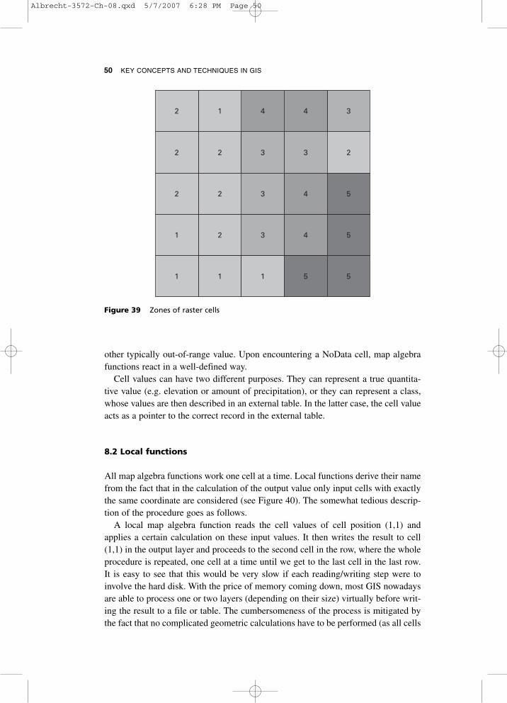
50 KEY CONCEPTS AND TECHNIQUES IN GIS
other typically out-of-range value. Upon encountering a NoData cell, map algebrafunctions react in a well-defined way.
Cell values can have two different purposes. They can represent a true quantita-tive value (e.g. elevation or amount of precipitation), or they can represent a class,whose values are then described in an external table. In the latter case, the cell valueacts as a pointer to the correct record in the external table.
8.2 Local functions
All map algebra functions work one cell at a time. Local functions derive their namefrom the fact that in the calculation of the output value only input cells with exactlythe same coordinate are considered (see Figure 40). The somewhat tedious descrip-tion of the procedure goes as follows.
A local map algebra function reads the cell values of cell position (1,1) andapplies a certain calculation on these input values. It then writes the result to cell(1,1) in the output layer and proceeds to the second cell in the row, where the wholeprocedure is repeated, one cell at a time until we get to the last cell in the last row.It is easy to see that this would be very slow if each reading/writing step were toinvolve the hard disk. With the price of memory coming down, most GIS nowadaysare able to process one or two layers (depending on their size) virtually before writ-ing the result to a file or table. The cumbersomeness of the process is mitigated bythe fact that no complicated geometric calculations have to be performed (as all cells
2 1 4 4 3
2 2 3 3 2
2 2 3 4 5
1 2 3 4 5
1 1 1 5 5
Figure 39 Zones of raster cells
Albrecht-3572-Ch-08.qxd 5/7/2007 6:28 PM Page 50
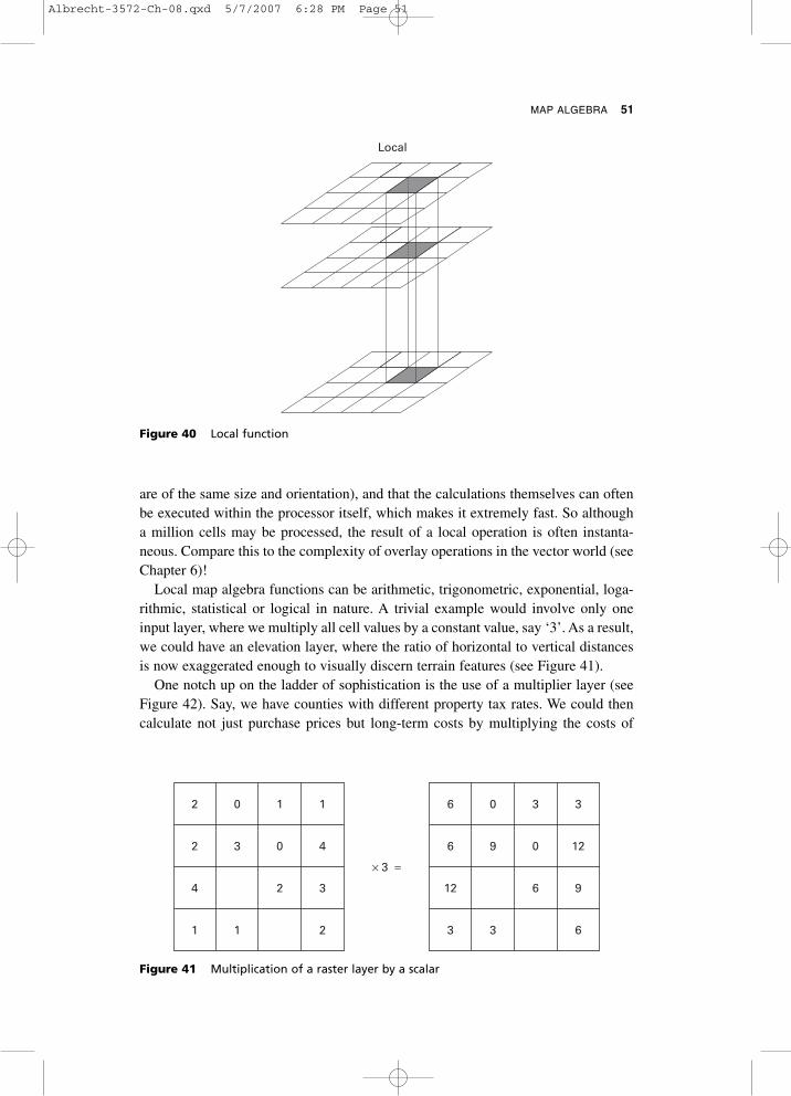
MAP ALGEBRA 51
2 0 1 1
2 3 0 4
4 2 3
1 1 2
6 0 3 3
6 9 0 12
12 6 9
3 3 6
× 3 =
Figure 41 Multiplication of a raster layer by a scalar
are of the same size and orientation), and that the calculations themselves can oftenbe executed within the processor itself, which makes it extremely fast. So althougha million cells may be processed, the result of a local operation is often instanta-neous. Compare this to the complexity of overlay operations in the vector world (seeChapter 6)!
Local map algebra functions can be arithmetic, trigonometric, exponential, loga-rithmic, statistical or logical in nature. A trivial example would involve only oneinput layer, where we multiply all cell values by a constant value, say ‘3’. As a result,we could have an elevation layer, where the ratio of horizontal to vertical distancesis now exaggerated enough to visually discern terrain features (see Figure 41).
One notch up on the ladder of sophistication is the use of a multiplier layer (seeFigure 42). Say, we have counties with different property tax rates. We could thencalculate not just purchase prices but long-term costs by multiplying the costs of
Local
Figure 40 Local function
Albrecht-3572-Ch-08.qxd 5/7/2007 6:28 PM Page 51

52 KEY CONCEPTS AND TECHNIQUES IN GIS
each property by the tax rates. Observe what happens to the cells with no values;NoData times something results in NoData.
8.3 Focal functions
Neighborhood or focal functions are the main reason for the success of map alge-bra. Local functions, in a way, are nothing but fancy recoding operations, whichcould indeed easily be performed in a proper database management system. Focalfunctions, on the other hand, take into account all cells in a user-defined neighbor-hood. Anybody who ever tried to calculate a cell value in a spreadsheet based on acombination of surrounding cells knows that the query string very fast becomesreally complicated. Again, the procedure is one cell at a time, except that for thecalculating of an output cell value, we now look at all cells surrounding the process-ing location of all input layers (see Figure 43).
2 0 1 1
2 3 0 4
4 2 3
1 1 2
6 0 3 3
6 9 0 12
12 6 9
3 3 6
12 0 3 3
12 27 0 48
48 12 27
3 3 12
× =
Figure 42 Multiplying one layer by another one
Focal
Figure 43 Focal function
Albrecht-3572-Ch-08.qxd 5/7/2007 6:28 PM Page 52
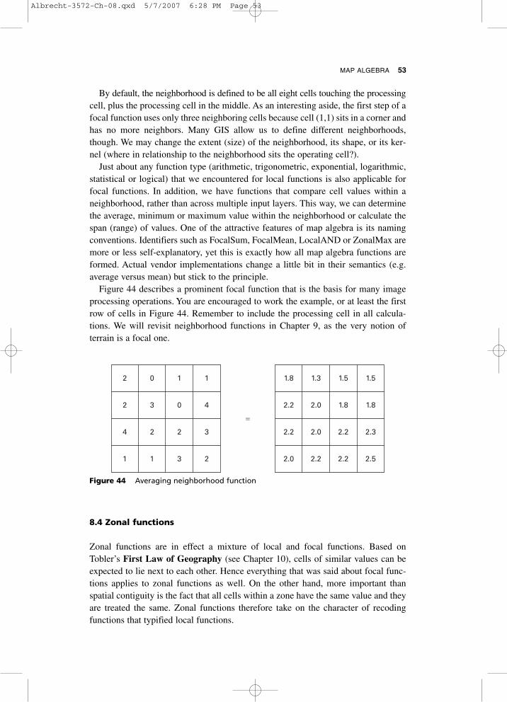
By default, the neighborhood is defined to be all eight cells touching the processingcell, plus the processing cell in the middle. As an interesting aside, the first step of afocal function uses only three neighboring cells because cell (1,1) sits in a corner andhas no more neighbors. Many GIS allow us to define different neighborhoods,though. We may change the extent (size) of the neighborhood, its shape, or its ker-nel (where in relationship to the neighborhood sits the operating cell?).
Just about any function type (arithmetic, trigonometric, exponential, logarithmic,statistical or logical) that we encountered for local functions is also applicable forfocal functions. In addition, we have functions that compare cell values within aneighborhood, rather than across multiple input layers. This way, we can determinethe average, minimum or maximum value within the neighborhood or calculate thespan (range) of values. One of the attractive features of map algebra is its namingconventions. Identifiers such as FocalSum, FocalMean, LocalAND or ZonalMax aremore or less self-explanatory, yet this is exactly how all map algebra functions areformed. Actual vendor implementations change a little bit in their semantics (e.g.average versus mean) but stick to the principle.
Figure 44 describes a prominent focal function that is the basis for many imageprocessing operations. You are encouraged to work the example, or at least the firstrow of cells in Figure 44. Remember to include the processing cell in all calcula-tions. We will revisit neighborhood functions in Chapter 9, as the very notion ofterrain is a focal one.
MAP ALGEBRA 53
2 0 1 1
2 3 0 4
4 2 2 3
31 1 2
1.8 1.3 1.5 1.5
2.2 2.0 1.8 1.8
2.2 2.0 2.2 2.3
2.0 2.2 2.2 2.5
=
Figure 44 Averaging neighborhood function
8.4 Zonal functions
Zonal functions are in effect a mixture of local and focal functions. Based onTobler’s First Law of Geography (see Chapter 10), cells of similar values can beexpected to lie next to each other. Hence everything that was said about focal func-tions applies to zonal functions as well. On the other hand, more important thanspatial contiguity is the fact that all cells within a zone have the same value and theyare treated the same. Zonal functions therefore take on the character of recodingfunctions that typified local functions.
Albrecht-3572-Ch-08.qxd 5/7/2007 6:28 PM Page 53
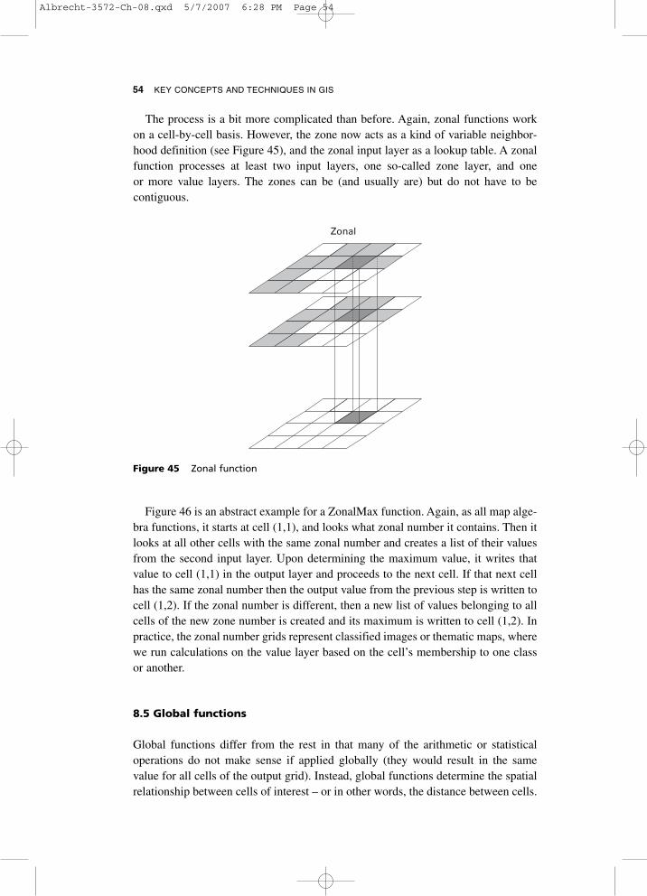
The process is a bit more complicated than before. Again, zonal functions workon a cell-by-cell basis. However, the zone now acts as a kind of variable neighbor-hood definition (see Figure 45), and the zonal input layer as a lookup table. A zonalfunction processes at least two input layers, one so-called zone layer, and oneor more value layers. The zones can be (and usually are) but do not have to becontiguous.
54 KEY CONCEPTS AND TECHNIQUES IN GIS
Zonal
Figure 45 Zonal function
Figure 46 is an abstract example for a ZonalMax function. Again, as all map alge-bra functions, it starts at cell (1,1), and looks what zonal number it contains. Then itlooks at all other cells with the same zonal number and creates a list of their valuesfrom the second input layer. Upon determining the maximum value, it writes thatvalue to cell (1,1) in the output layer and proceeds to the next cell. If that next cellhas the same zonal number then the output value from the previous step is written tocell (1,2). If the zonal number is different, then a new list of values belonging to allcells of the new zone number is created and its maximum is written to cell (1,2). Inpractice, the zonal number grids represent classified images or thematic maps, wherewe run calculations on the value layer based on the cell’s membership to one classor another.
8.5 Global functions
Global functions differ from the rest in that many of the arithmetic or statisticaloperations do not make sense if applied globally (they would result in the samevalue for all cells of the output grid). Instead, global functions determine the spatialrelationship between cells of interest – or in other words, the distance between cells.
Albrecht-3572-Ch-08.qxd 5/7/2007 6:28 PM Page 54
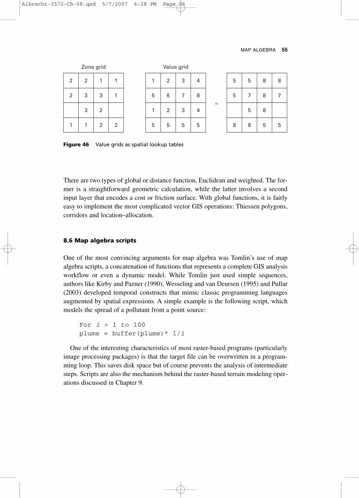
There are two types of global or distance function, Euclidean and weighted. The for-mer is a straightforward geometric calculation, while the latter involves a secondinput layer that encodes a cost or friction surface. With global functions, it is fairlyeasy to implement the most complicated vector GIS operations: Thiessen polygons,corridors and location–allocation.
8.6 Map algebra scripts
One of the most convincing arguments for map algebra was Tomlin’s use of mapalgebra scripts, a concatenation of functions that represents a complete GIS analysisworkflow or even a dynamic model. While Tomlin just used simple sequences,authors like Kirby and Pazner (1990), Wesseling and van Deursen (1995) and Pullar(2003) developed temporal constructs that mimic classic programming languagesaugmented by spatial expressions. A simple example is the following script, whichmodels the spread of a pollutant from a point source:
For i = 1 to 100plume = buffer(plume)* 1/i
One of the interesting characteristics of most raster-based programs (particularlyimage processing packages) is that the target file can be overwritten in a program-ming loop. This saves disk space but of course prevents the analysis of intermediatesteps. Scripts are also the mechanism behind the raster-based terrain modeling oper-ations discussed in Chapter 9.
MAP ALGEBRA 55
2 2 1 1
2 3 3 1
23
1 1 22
1 2 3 4
5 6 7 8
1 2 3 4
5 5 5 5
5 5 8 8
5 7 8 7
85
8 8 55
=
Zone grid Value grid
Figure 46 Value grids as spatial lookup tables
Albrecht-3572-Ch-08.qxd 5/7/2007 6:28 PM Page 55

All GIS functionality discussed so far assumed the world to be flat. This is, ofcourse, utterly unrealistic but GIS has succeeded in getting away with this deficiencysurprisingly well. Since 3-D representations are commonplace in modern CAD soft-ware, the obvious question is why has GIS not followed suit. The answer lies in thedistinction between mere data representation that is common to CAD and vectorGIS, on the one hand, and the spatial reasoning capacity that is unique to GIS.
In general, we can distinguish between three different ways to represent the thirddimension (see Figure 47). One is the use of true three-dimensional coordinates toconstruct what in CAD is called a wire frame model. The second uses the samecoordinates but constructs a mesh of triangles to drape a surface going through allthe points. Applied to relatively small areas but at high precision, this data structureis often used in civil engineering applications. The last uses raster cells and recordsfor each cell an elevation value as the pertinent attribute. The image of the rastersurface in Figure 47 indicates a fourth representation, the use of contour lines. Theyare a filter on the former, leaving only values at certain intervals, which are then con-nected by a polyline. As we have seen earlier, the way we organize data directlydetermines what kind of questions we can ask of the data. The wire frame model isup to now the most limited of 3-D GIS models, serving mostly rendering functionssimilar to those of architectural software packages.
9 TERRAIN MODELING
3-D Wire frame
Raster Surface
Snow Depth
Tin
Figure 47 Three ways to represent the third dimension
Albrecht-3572-Ch-09.qxd 5/7/2007 6:30 PM Page 56
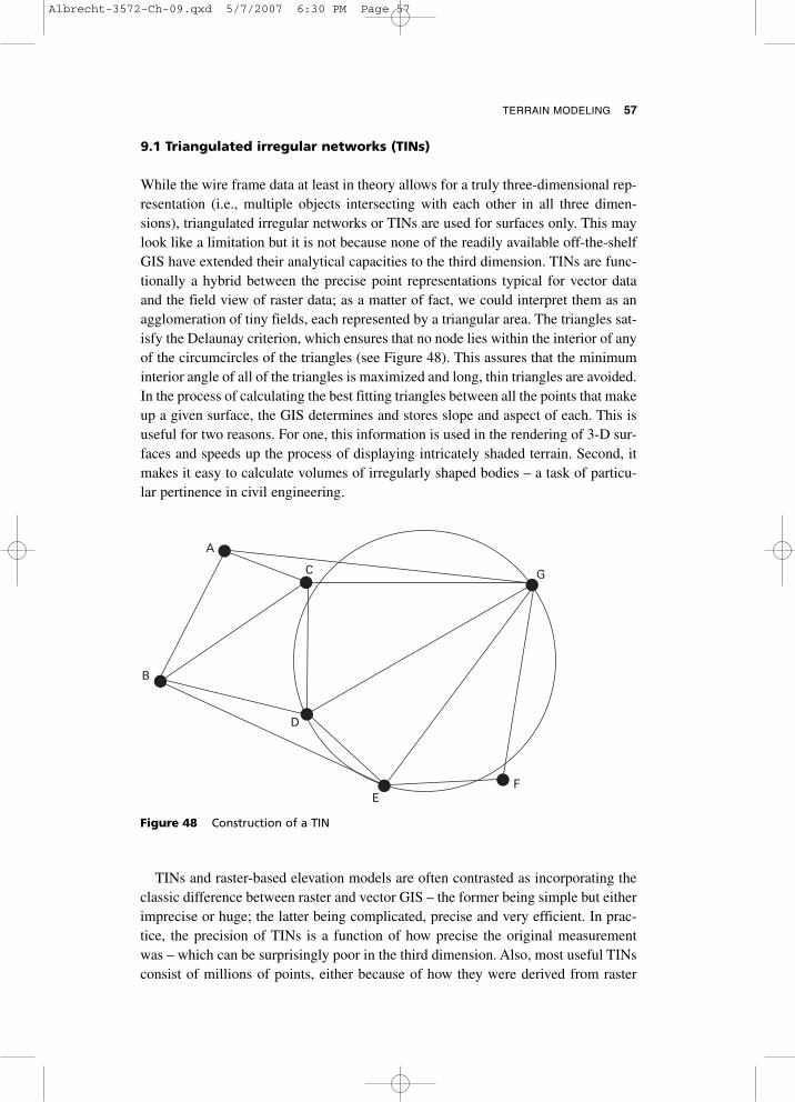
TERRAIN MODELING 57
9.1 Triangulated irregular networks (TINs)
While the wire frame data at least in theory allows for a truly three-dimensional rep-resentation (i.e., multiple objects intersecting with each other in all three dimen-sions), triangulated irregular networks or TINs are used for surfaces only. This maylook like a limitation but it is not because none of the readily available off-the-shelfGIS have extended their analytical capacities to the third dimension. TINs are func-tionally a hybrid between the precise point representations typical for vector dataand the field view of raster data; as a matter of fact, we could interpret them as anagglomeration of tiny fields, each represented by a triangular area. The triangles sat-isfy the Delaunay criterion, which ensures that no node lies within the interior of anyof the circumcircles of the triangles (see Figure 48). This assures that the minimuminterior angle of all of the triangles is maximized and long, thin triangles are avoided.In the process of calculating the best fitting triangles between all the points that makeup a given surface, the GIS determines and stores slope and aspect of each. This isuseful for two reasons. For one, this information is used in the rendering of 3-D sur-faces and speeds up the process of displaying intricately shaded terrain. Second, itmakes it easy to calculate volumes of irregularly shaped bodies – a task of particu-lar pertinence in civil engineering.
G
FE
D
C
A
B
Figure 48 Construction of a TIN
TINs and raster-based elevation models are often contrasted as incorporating theclassic difference between raster and vector GIS – the former being simple but eitherimprecise or huge; the latter being complicated, precise and very efficient. In prac-tice, the precision of TINs is a function of how precise the original measurementwas – which can be surprisingly poor in the third dimension. Also, most useful TINsconsist of millions of points, either because of how they were derived from raster
Albrecht-3572-Ch-09.qxd 5/7/2007 6:30 PM Page 57
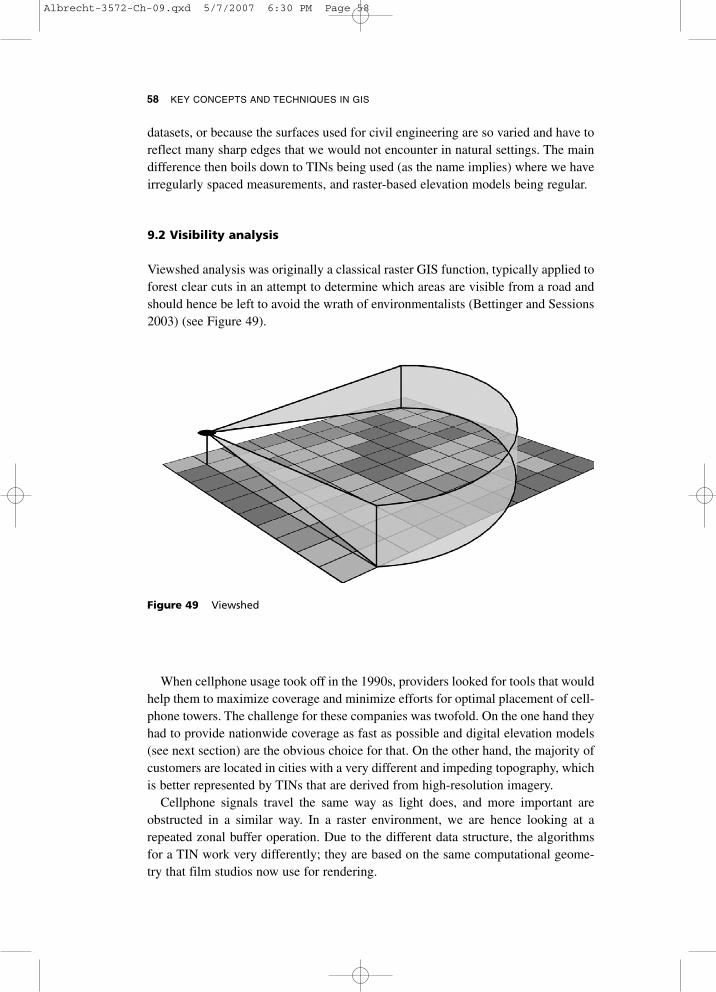
datasets, or because the surfaces used for civil engineering are so varied and have toreflect many sharp edges that we would not encounter in natural settings. The maindifference then boils down to TINs being used (as the name implies) where we haveirregularly spaced measurements, and raster-based elevation models being regular.
9.2 Visibility analysis
Viewshed analysis was originally a classical raster GIS function, typically applied toforest clear cuts in an attempt to determine which areas are visible from a road andshould hence be left to avoid the wrath of environmentalists (Bettinger and Sessions2003) (see Figure 49).
58 KEY CONCEPTS AND TECHNIQUES IN GIS
Figure 49 Viewshed
When cellphone usage took off in the 1990s, providers looked for tools that wouldhelp them to maximize coverage and minimize efforts for optimal placement of cell-phone towers. The challenge for these companies was twofold. On the one hand theyhad to provide nationwide coverage as fast as possible and digital elevation models(see next section) are the obvious choice for that. On the other hand, the majority ofcustomers are located in cities with a very different and impeding topography, whichis better represented by TINs that are derived from high-resolution imagery.
Cellphone signals travel the same way as light does, and more important areobstructed in a similar way. In a raster environment, we are hence looking at arepeated zonal buffer operation. Due to the different data structure, the algorithmsfor a TIN work very differently; they are based on the same computational geome-try that film studios now use for rendering.
Albrecht-3572-Ch-09.qxd 5/7/2007 6:30 PM Page 58

9.3 Digital elevation and terrain models
Raster-based digital elevation models (DEMs) are by far the most common basis fordealing with the third dimension. As a matter of fact, many people have difficultiesconceptualizing a raster attribute as anything but elevation. This is especially true fordigital elevation models that cover larger areas. There are two reasons for this. Forone, automated data capture for large areas tends to involve remote sensing methodsthat result in raster datasets. As important, however, is the fact that map algebraoffers a plethora of analytical methods that require nothing but elevation and resultin an astounding array of derivatives.
In Chapter 8, we saw how focal or neighborhood operations are used to analyzethe combined spatial and attribute relationship between locations. The first set offocal operations transforms a DEM to a digital terrain model or DTM. The differ-ence between the two is that the latter stores, in addition to mere elevation, twoimportant derivatives – slope and aspect (see Figure 50). Slope is the ratio of eleva-tion difference between the higher neighbors and the lower neighbors, and horizon-tal distance between those neighbors. It is usually calculated based on the8-neighborhood, which in turn defines the distance as twice the cell width in thecardinal directions, and <surd>2 times the former distance for the diagonals. Oncewe know the slope at each cell location, it is another simple focal operation to com-pare all neighbors and determine in what direction the surface slopes; this is calledaspect. Given that both operations are fairly simple, and that processing power ofmodern computers is sufficient to calculate slope and aspect efficiently, DTMs aredecreasing in importance.
TERRAIN MODELING 59
Aspect
Slope
36%
20°
14°
8.5°
2.9°1.1°
25%
15%5%
0
45
90
135
180
225
270
315
2%
Figure 50 Derivation of slope and aspect
Albrecht-3572-Ch-09.qxd 5/7/2007 6:30 PM Page 59
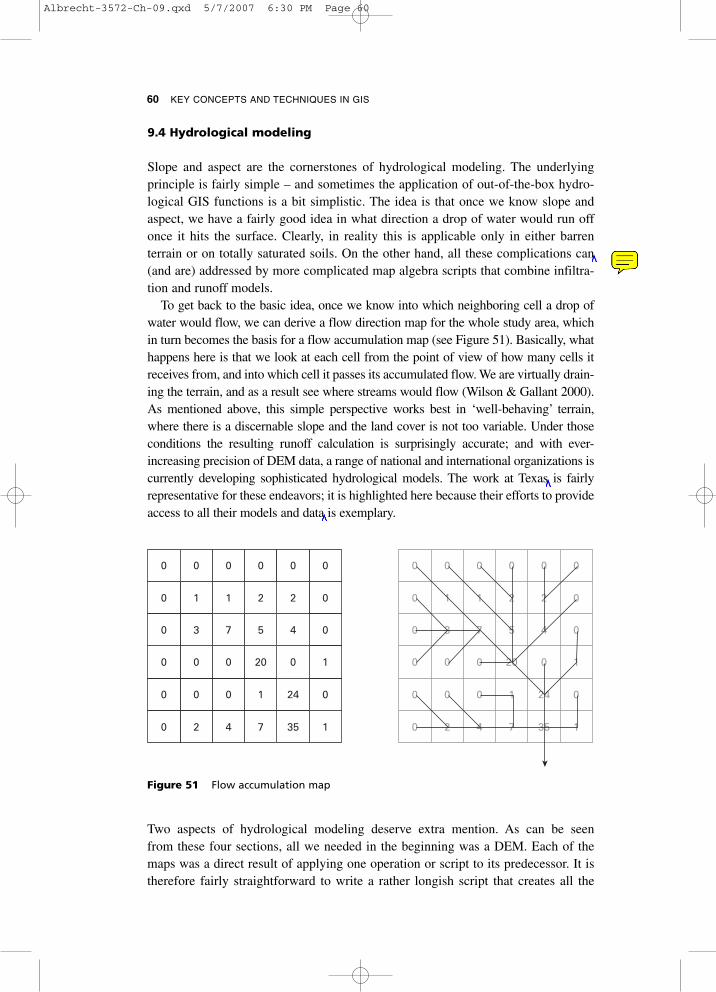
9.4 Hydrological modeling
Slope and aspect are the cornerstones of hydrological modeling. The underlyingprinciple is fairly simple – and sometimes the application of out-of-the-box hydro-logical GIS functions is a bit simplistic. The idea is that once we know slope andaspect, we have a fairly good idea in what direction a drop of water would run offonce it hits the surface. Clearly, in reality this is applicable only in either barrenterrain or on totally saturated soils. On the other hand, all these complications can(and are) addressed by more complicated map algebra scripts that combine infiltra-tion and runoff models.
To get back to the basic idea, once we know into which neighboring cell a drop ofwater would flow, we can derive a flow direction map for the whole study area, whichin turn becomes the basis for a flow accumulation map (see Figure 51). Basically, whathappens here is that we look at each cell from the point of view of how many cells itreceives from, and into which cell it passes its accumulated flow. We are virtually drain-ing the terrain, and as a result see where streams would flow (Wilson & Gallant 2000).As mentioned above, this simple perspective works best in ‘well-behaving’ terrain,where there is a discernable slope and the land cover is not too variable. Under thoseconditions the resulting runoff calculation is surprisingly accurate; and with ever-increasing precision of DEM data, a range of national and international organizations iscurrently developing sophisticated hydrological models. The work at Texas is fairlyrepresentative for these endeavors; it is highlighted here because their efforts to provideaccess to all their models and data is exemplary.
60 KEY CONCEPTS AND TECHNIQUES IN GIS
0 0 0 0 0 0
0 1 1 2 2 0
0 3 7 5 4 0
0 0 0 20 0 1
0 0 0 1 24 0
0 2 4 7 35 1
0 0 0 0 0 0
0 1 1 2 2 0
0 3 7 5 4 0
0 0 0 20 0 1
0 0 0 1 24 0
0 2 4 7 35 1
Figure 51 Flow accumulation map
Two aspects of hydrological modeling deserve extra mention. As can be seenfrom these four sections, all we needed in the beginning was a DEM. Each of themaps was a direct result of applying one operation or script to its predecessor. It istherefore fairly straightforward to write a rather longish script that creates all the
Albrecht-3572-Ch-09.qxd 5/7/2007 6:30 PM Page 60

intermediate files and derives a flood forecast model in one go – a prime examplefor the power of map algebra. Second, impressive as all of this is, it provides only ahint at all the models that can be developed and linked with each other. For exam-ple, based on a comparison of satellite images, we can develop models of urbansprawl and impervious surfaces. These can then be linked with the runoff modelabove to develop true simulation models, possibly linked with real-time readings ofprecipitation.
All of the above are true terrain modeling applications. The methods discussed inthis chapter are, however, just as applicable to artificial surfaces, where the thirddimension represents an attribute value such as property value or air pollution. Thesekinds of surfaces are typically interpolated from sparse measurements. The follow-ing chapter will cover spatial interpolation techniques and more.
TERRAIN MODELING 61
Albrecht-3572-Ch-09.qxd 5/7/2007 6:30 PM Page 61

This chapter consists of two distinct parts because the phrase ‘spatial statistics’ hastwo rather different meanings depending where one comes from. The first comesfrom a geophysics background and is also known as geo-statistics. The second hasits roots in analytical cartography and is known as spatial analysis.
10.1 Geo-statistics
Typically, stochastic methods are applied when we have lots of data but not a reallygood idea of what drives the data. Deterministic models, on the other hand, are usedwhen the data is sparse but we are confident that our understanding of the phenom-enon, say based on a long history of similar observations, is good. The following setof methods cover both approaches, although the underlying commonality is ascarcity of data. All spatial interpolation techniques discussed here aim at creatingsurfaces from point data. It is important to recognize that most applications are notin terrain modeling but that the surfaces are intended to allow estimates of any kindof continuous variable, such as pollution, crime or mineral resources.
All model-based interpolation methods assume Tobler’s (1970) First Law ofGeography, which basically means that everything is related to everything else, butthings that are closer in space (i.e., neighbors) are also closer with respect to theirattribute values. There are many interpolation methods and we use some descriptorsto categorize them by the number of input values (local versus global methods) andthe characteristics of the resulting surface. If the surface goes through the values ofknown locations, then we label a method as exact. Otherwise we refer to it as asmooth interpolator, because the resulting surface avoids ruggedness around meas-ured locations. The most common of these methods are inverse distance weighting(IDW), polynomials and splines.
10.1.1 Inverse distance weightingIDW is the most direct implementation of Tobler’s First Law (see Figure 52). Givenknown values at some locations, we try to determine the most probable value at alocation for which we don’t have a measurement.
The calculation is made up of known values of neighboring locations, which areweighted according to their distance from the one location for which we want todetermine a value. This calculation is repeated for as many points as we care about.If the surface to be created is based on a TIN data structure, then we probably onlydouble or triple the number of original points. If the surface is a raster dataset, then
10 SPATIAL STATISTICS
Albrecht-3572-Ch-10.qxd 5/7/2007 6:11 PM Page 62
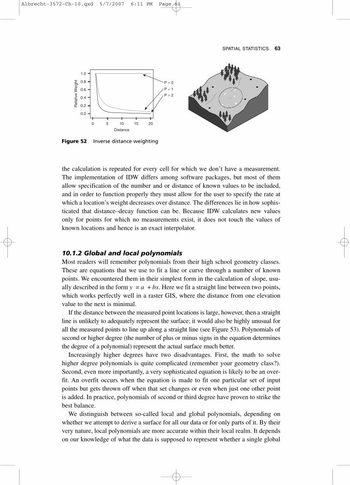
SPATIAL STATISTICS 63
the calculation is repeated for every cell for which we don’t have a measurement.The implementation of IDW differs among software packages, but most of themallow specification of the number and or distance of known values to be included,and in order to function properly they must allow for the user to specify the rate atwhich a location’s weight decreases over distance. The differences lie in how sophis-ticated that distance–decay function can be. Because IDW calculates new valuesonly for points for which no measurements exist, it does not touch the values ofknown locations and hence is an exact interpolator.
10.1.2 Global and local polynomialsMost readers will remember polynomials from their high school geometry classes.These are equations that we use to fit a line or curve through a number of knownpoints. We encountered them in their simplest form in the calculation of slope, usu-ally described in the form y = a + bx. Here we fit a straight line between two points,which works perfectly well in a raster GIS, where the distance from one elevationvalue to the next is minimal.
If the distance between the measured point locations is large, however, then a straightline is unlikely to adequately represent the surface; it would also be highly unusual forall the measured points to line up along a straight line (see Figure 53). Polynomials ofsecond or higher degree (the number of plus or minus signs in the equation determinesthe degree of a polynomial) represent the actual surface much better.
Increasingly higher degrees have two disadvantages. First, the math to solvehigher degree polynomials is quite complicated (remember your geometry class?).Second, even more importantly, a very sophisticated equation is likely to be an over-fit. An overfit occurs when the equation is made to fit one particular set of inputpoints but gets thrown off when that set changes or even when just one other pointis added. In practice, polynomials of second or third degree have proven to strike thebest balance.
We distinguish between so-called local and global polynomials, depending onwhether we attempt to derive a surface for all our data or for only parts of it. By theirvery nature, local polynomials are more accurate within their local realm. It dependson our knowledge of what the data is supposed to represent whether a single global
P = 0
P = 1
P = 2
2015105
Rel
ativ
e W
eigh
t
Distance
0
1.0
0.8
0.6
0.4
0.2
0.0
Figure 52 Inverse distance weighting
Albrecht-3572-Ch-10.qxd 5/7/2007 6:11 PM Page 63
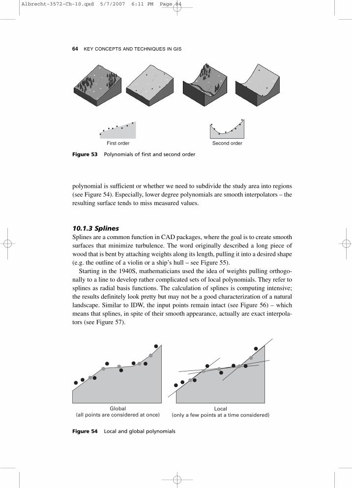
polynomial is sufficient or whether we need to subdivide the study area into regions(see Figure 54). Especially, lower degree polynomials are smooth interpolators – theresulting surface tends to miss measured values.
10.1.3 SplinesSplines are a common function in CAD packages, where the goal is to create smoothsurfaces that minimize turbulence. The word originally described a long piece ofwood that is bent by attaching weights along its length, pulling it into a desired shape(e.g. the outline of a violin or a ship’s hull – see Figure 55).
Starting in the 1940S, mathematicians used the idea of weights pulling orthogo-nally to a line to develop rather complicated sets of local polynomials. They refer tosplines as radial basis functions. The calculation of splines is computing intensive;the results definitely look pretty but may not be a good characterization of a naturallandscape. Similar to IDW, the input points remain intact (see Figure 56) – whichmeans that splines, in spite of their smooth appearance, actually are exact interpola-tors (see Figure 57).
64 KEY CONCEPTS AND TECHNIQUES IN GIS
First order Second order
Figure 53 Polynomials of first and second order
Global(all points are considered at once)
Local(only a few points at a time considered)
Figure 54 Local and global polynomials
Albrecht-3572-Ch-10.qxd 5/7/2007 6:11 PM Page 64
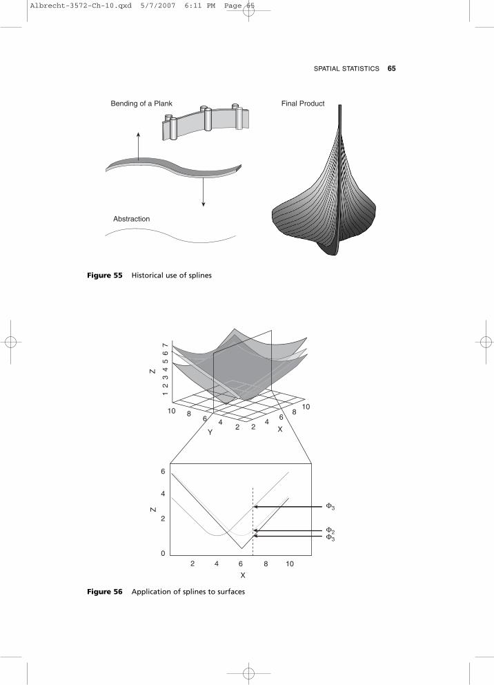
SPATIAL STATISTICS 65
Bending of a Plank
Abstraction
Final Product
Figure 55 Historical use of splines
1
10 108 8
6
6
6
X
8 10
6
XY4
4
4
42
2
20
2
23
4ZZ
56
7
Φ3
Φ2Φ3
Figure 56 Application of splines to surfaces
Albrecht-3572-Ch-10.qxd 5/7/2007 6:11 PM Page 65

10.1.4 KrigingAll of the above interpolation methods use a model of what the analyst believes isthe best representation of the interpolated surface. Kriging does this too; however,it uses statistics to develop the model. Originally developed for applications in themining industry, it is now widely used in epidemiology, the environmental sciences,and of course geophysics. The term ‘kriging’ now signifies a whole family of meth-ods, which to explain would go way beyond the scope of this book. The following istherefore only a general description of what underlies all kriging methods.
Kriging adopts the simple polynomial view of the world but concentrates on thetail end of the equation – called error – that describes what is not captured by theequation proper. In
y = a + bx + cx2 + e
for instance, we have a second-degree polynomial with an error term e, which basicallyis a vessel for all discrepancies between the model result and the observed outcome(remember, polynomials are smooth or inexact interpolators). Using the First Law ofGeography, it is now fair to assume that all the errors are spatially autocorrelated –that is, they increase the further we get away from a measured point. Kriging uses abrute force method of computing the relationships between all measured points andthen runs statistics over the resulting table to determine which points have how muchinfluence on what other points. This information is then fed back into the surface equa-tion, which ideally is then error-free, making kriging an exact interpolator.
In practice there are a number of complications, each of which is addressed by aparticular kind of kriging method. Especially the more sophisticated forms of krig-ing are extremely computing intensive; the results are no great shake if the numberof original measurements is too small and the calculations row out of bounds if wehave a rich input dataset. For the right number of points, and if the computing poweris available, kriging delivers very robust results.
66 KEY CONCEPTS AND TECHNIQUES IN GIS
Exact:never exceeding
given values
Exact:possibly exaggerating
Figure 57 Exact and inexact interpolators
Albrecht-3572-Ch-10.qxd 5/7/2007 6:11 PM Page 66

SPATIAL STATISTICS 67
10.2 Spatial analysis
Spatial analysis comprises of a whole bag of different methods dealing with thequantitative analysis of spatial data. It ranges from simple geometric descriptors tohighly sophisticated spatial interaction models. In a narrow sense, spatial analysis isthe decidedly pre-GIS set of methods developed by geographers during the quanti-tative revolution of the 1960s, who in turn borrowed from analytical cartographers.Their goal was to describe geographic distributions, identify spatial patterns, andanalyze geographic relationships and processes – all without GIS and often enougheven without anything close to a computer.
10.2.1 Geometric descriptorsThis is the application of descriptive statistics to spatial data. While we may some-times borrow directly from traditional statistics, more often than not spatial alsomeans special. In other words, we will have to come up with procedures that capturethe spirit of what the traditional methods try to accomplish but adjust their imple-mentation to the multi-dimensionality of spatial data, and possibly more importantto the fact that we cannot assume spatial samples to be independent of each other.
We referred to the phenomenon of spatial autocorrelation above but did notexpand on what a nuisance it poses for the statistical analysis of spatial data.Traditional statistics is based on the fact that samples are taken independently ofeach other and most methods assume a normal distribution. Both of these assump-tions do not hold with geographic data – if they did, then there would be no basis forthe discipline of geography. If a distribution is random then it is decidedly non-geographic, and Tobler’s First Law of Geography would not hold.
The most basic descriptors in traditional statistics are mean, mode and standarddeviation. Of these, the mean is relatively easy to translate into a spatial context; wejust have to make sure that we calculate the average along as many dimensions(typically 1 to 3 for transects, areas or volumes) as we need. Figure 58 gives anexample of a geometric mean.
The geometric median is a bit different from its traditional counterpart.Calculating the median values along x, y and possibly z to then mark the medianlocation does not capture what we usually strive for in the calculation of a median.In traditional statistics, the median marks the point that is as far away from one endof the distribution as from the other. Translated into the spatial realm, this meansthat we are looking for a location that does the same not just within a dimension butalso across. As it turns out, this is a really useful measure because it describes thelocation that minimizes the combined distances from that central point to all otherlocations. Unfortunately, there is no simple equation for that – the point can be foundonly through iterative optimization. Figure 59 illustrates the difference between aspatial mean and a spatial median.
A simple measure of central tendency is often too crude to adequately describe ageographic distribution. Analogue to the standard deviation in traditional statistics,
Albrecht-3572-Ch-10.qxd 5/7/2007 6:11 PM Page 67

we can employ standard distance as the circle around the mean, which captures a sig-nificant number of neighbors. The smaller the circle the more compact is the phe-nomenon; a wide circle tells us that the spatial mean is not very representative.However, by just calculating the standard distance, we throw away a lot of additionalinformation. If we separate the standard distance into its x and y components, we geta standard deviational eclipse (see Figure 60) that tells us about the orientation ordirection of the phenomenon and hence gives us additional clues as to what causesor at least influences it. This even applies to linear features, as a multitude of pathsdistributed over a larger surface (e.g. hurricanes or a river network) provides valu-able clues as to what forces a change in direction.
The field of spatial pattern descriptors was expanded by landscape ecologists inthe 1980s, who developed a myriad of measures to describe shapes and geometricrelationships between features. Shape measures (see Figure 61) try to come up withcharacteristic numbers such as the ratio of edge length to area size, the degree ofroundness (with a circle being perfectly round), or a figure for a feature’s fractaldimension. While we will discuss more advanced spatial relationships in the nextsection, it is worthwhile to mention that a number of landscape ecological measurescalculate average, min and max distance between features in general and on a fea-ture class by feature class basis.
68 KEY CONCEPTS AND TECHNIQUES IN GIS
22
20
18
16
14
12
10
8
6
4
2
2 4 6 8 10 12 14 16 18 20 22
Figure 58 Geometric mean
Albrecht-3572-Ch-10.qxd 5/7/2007 6:11 PM Page 68
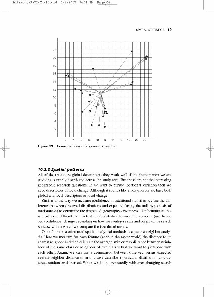
10.2.2 Spatial patternsAll of the above are global descriptors; they work well if the phenomenon we arestudying is evenly distributed across the study area. But those are not the interestinggeographic research questions. If we want to pursue locational variation then weneed descriptors of local change. Although it sounds like an oxymoron, we have bothglobal and local descriptors or local change.
Similar to the way we measure confidence in traditional statistics, we use the dif-ference between observed distributions and expected (using the null hypothesis ofrandomness) to determine the degree of ‘geography-drivenness’. Unfortunately, thisis a bit more difficult than in traditional statistics because the numbers (and henceour confidence) change depending on how we configure size and origin of the searchwindow within which we compare the two distributions.
One of the most often used spatial analytical methods is a nearest-neighbor analy-sis. Here we measure for each feature (zone in the raster world) the distance to itsnearest neighbor and then calculate the average, min or max distance between neigh-bors of the same class or neighbors of two classes that we want to juxtapose witheach other. Again, we can use a comparison between observed versus expectednearest-neighbor distance to in this case describe a particular distribution as clus-tered, random or dispersed. When we do this repeatedly with ever-changing search
SPATIAL STATISTICS 69
22
20
18
16
14
12
10
8
6
4
2
2 4 6 8 10 12 14 16 18 20 22
Figure 59 Geometric mean and geometric median
Albrecht-3572-Ch-10.qxd 5/7/2007 6:11 PM Page 69

window size, we find the scale at which a given spatial pattern is particularly promi-nent, which in turn helps us to identify the process that is driving the spatial pattern.
So far, we have assumed that all features either belonged to one and the same classor to a limited number of classes, for which we then describe the respective spatial
70 KEY CONCEPTS AND TECHNIQUES IN GIS
22
20
18
16
14
12
10
8
6
4
2
2 4 6 8 10 12 14 16 18 20 22
Figure 60 Standard deviational ellipse
High Value
Low Value
Area Edge Shape DiversityCoreArea
NearestNeighbor
PatchDensity
Figure 61 Shape measures
Albrecht-3572-Ch-10.qxd 5/7/2007 6:11 PM Page 70
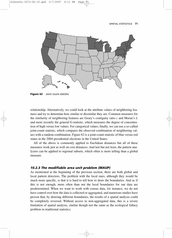
relationship. Alternatively, we could look at the attribute values of neighboring fea-tures and try to determine how similar or dissimilar they are. Common measures forthe similarity of neighboring features are Geary’s contiguity ratio c and Moran’s I,and more recently the general G-statistic, which measures the degree of concentra-tion of high versus low values. For categorical values, finally, we can use a so-calledjoint-count statistic, which compares the observed combination of neighboring val-ues with a random combination. Figure 62 is a joint-count statistic of blue versus redstates in the 2004 presidential elections in the United States.
All of the above is commonly applied to Euclidean distances but all of thesemeasures work just as well on cost distances. And last but not least, the pattern ana-lyzers can be applied to regional subsets, which often is more telling than a globalmeasure.
10.2.3 The modifiable area unit problem (MAUP)As mentioned at the beginning of the previous section, there are both global andlocal pattern detectors. The problem with the local ones, although they would bemuch more specific, is that it is hard to tell how to draw the boundaries. And as ifthis is not enough, more often than not the local boundaries for our data arepredetermined. When we want to work with census data, for instance, we do nothave control over how the data is collected or aggregated, and numerous studies haveproven that, by drawing different boundaries, the results of a spatial analysis couldbe completely reversed. Without access to non-aggregated data, this is a severelimitation of spatial analysis, similar though not the same as the ecological fallacyproblem in traditional statistics.
SPATIAL STATISTICS 71
Figure 62 Joint count statistic
Albrecht-3572-Ch-10.qxd 5/7/2007 6:11 PM Page 71

10.2.4 Geographic relationshipsAnother major contributor to spatial analysis techniques is the discipline of regionalscience, somewhat of a hybrid between economic geography and spatial economet-rics. Some of the network-based location–allocation models come out of that realm,but what interests us here is the use of systems of regression equations to representthese relationships between geographic features. The polynomials that we encoun-tered in geostatistics can be used the other way around – not to calculate missing val-ues but to determine the underlying forcing functions that result in the observedvalues. Although there are examples for global regression analysis, the local (alsoknown as geographically weighted) regression is of particular interest.
Many of these calculations are computationally very expensive, especiallybecause an unbiased analysis requires the repeated run of many scenarios, whereparameters are altered one at a time (Monte Carlo analysis). The frustration with thisPandora box of spatial analysis problems led to the development of geo-computationas a field, where the latest information science methods are applied to solvinguncomfortably large spatial analysis problems. We look at these in the next chapter.
72 KEY CONCEPTS AND TECHNIQUES IN GIS
Albrecht-3572-Ch-10.qxd 5/7/2007 6:11 PM Page 72

Geocomputation is a set of computational methods that has been customized toaddress the special characteristics of spatial data. Given that definition, GIS wouldbe a geocomputational method but it is decidedly not. The term was invented bygeographer Stan Openshaw and became institutionalized with the first GeoComputationconference in 1996. The term ‘computational’ has come to replace what used to beknown as artificial intelligence techniques: from genetic algorithms, neural net-works, and fuzzy reasoning to cellular automata, agent-based modeling, and highlyparallelized processing. The common ground behind all of these is that if we throwlots of processing power and the latest advances in information science at large spa-tial datasets, then we have a good shot at deriving new insights.
A look at the proceedings of the GeoComputation conference series (www.geo-computation.org) conveys the wide range of topics, far more than could be coveredin this chapter. We will concentrate here on five areas of research that have maturedmore than others: fuzzy reasoning, neural networks, genetic algorithms, cellularautomata and agent-based modeling systems.
11.1 Fuzzy reasoning
As mentioned above, geocomputational techniques are borrowed from informationscience and then applied to spatial data. Lofti Zadeh (1965) formalized a set of rulesto work with multi-valued logic, which allows us to capture the multi-valuedness ofour thinking. Rather than categorizing everything as yes/no, black/white, zero/oneetc., as we did when we introduced Boolean logic in Chapter 6, fuzzy logic extendsthe hard values zero and one to everything in between. An attribute can now be alittle bit of green and a little more of blue rather than either green or blue. Andapplied to geographic phenomena, Florida can be 10% tropical, 80% subtropical,and another 10% moderate in climate.
The best everyday illustration of how fuzziness works is a shower knob that thisauthor found in the bathroom of a New Zealand colleague (see Figure 63). Peopletend to have different opinions about what is warm water. By having the marking forcold water become ever thinner as the marking for warm water increases in width,the definition covers a wide range of beliefs with the majority somewhere in the mid-dle at around 45°centigrade.
11 GEOCOMPUTATION
Albrecht-3572-Ch-11.qxd 5/7/2007 6:10 PM Page 73
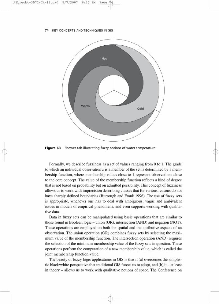
Formally, we describe fuzziness as a set of values ranging from 0 to 1. The gradeto which an individual observation z is a member of the set is determined by a mem-bership function, where membership values close to 1 represent observations closeto the core concept. The value of the membership function reflects a kind of degreethat is not based on probability but on admitted possibility. This concept of fuzzinessallows us to work with imprecision describing classes that for various reasons do nothave sharply defined boundaries (Burrough and Frank 1996). The use of fuzzy setsis appropriate, whenever one has to deal with ambiguous, vague and ambivalentissues in models of empirical phenomena, and even supports working with qualita-tive data.
Data in fuzzy sets can be manipulated using basic operations that are similar tothose found in Boolean logic – union (OR), intersection (AND) and negation (NOT).These operations are employed on both the spatial and the attributive aspects of anobservation. The union operation (OR) combines fuzzy sets by selecting the maxi-mum value of the membership function. The intersection operation (AND) requiresthe selection of the minimum membership value of the fuzzy sets in question. Theseoperations perform the computation of a new membership value, which is called thejoint membership function value.
The beauty of fuzzy logic applications in GIS is that it (a) overcomes the simplis-tic black/white perspective that traditional GIS forces us to adopt, and (b) it – at leastin theory – allows us to work with qualitative notions of space. The Conference on
74 KEY CONCEPTS AND TECHNIQUES IN GIS
Hot
WarmCold
Figure 63 Shower tab illustrating fuzzy notions of water temperature
Albrecht-3572-Ch-11.qxd 5/7/2007 6:10 PM Page 74
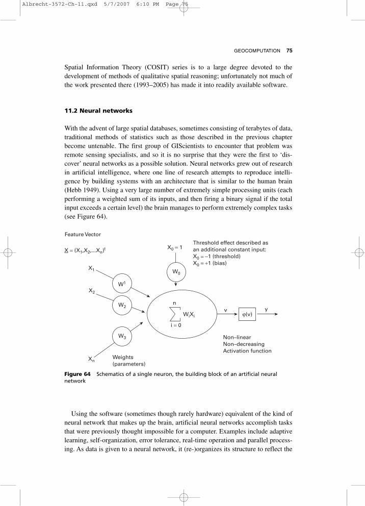
Spatial Information Theory (COSIT) series is to a large degree devoted to thedevelopment of methods of qualitative spatial reasoning; unfortunately not much ofthe work presented there (1993–2005) has made it into readily available software.
11.2 Neural networks
With the advent of large spatial databases, sometimes consisting of terabytes of data,traditional methods of statistics such as those described in the previous chapterbecome untenable. The first group of GIScientists to encounter that problem wasremote sensing specialists, and so it is no surprise that they were the first to ‘dis-cover’ neural networks as a possible solution. Neural networks grew out of researchin artificial intelligence, where one line of research attempts to reproduce intelli-gence by building systems with an architecture that is similar to the human brain(Hebb 1949). Using a very large number of extremely simple processing units (eachperforming a weighted sum of its inputs, and then firing a binary signal if the totalinput exceeds a certain level) the brain manages to perform extremely complex tasks(see Figure 64).
GEOCOMPUTATION 75
Feature Vector
Weights(parameters)
Non–linearNon–decreasingActivation function
Threshold effect described asan additional constant input:X0 = −1 (threshold)X0 = +1 (bias)
X = (X1,X2,...Xn)t X0 = 1
X1
X2
Xn
W1
W2
W3
W0
v yn
i = 0
WiXi ϕ(v)
Figure 64 Schematics of a single neuron, the building block of an artificial neuralnetwork
Using the software (sometimes though rarely hardware) equivalent of the kind ofneural network that makes up the brain, artificial neural networks accomplish tasksthat were previously thought impossible for a computer. Examples include adaptivelearning, self-organization, error tolerance, real-time operation and parallel process-ing. As data is given to a neural network, it (re-)organizes its structure to reflect the
Albrecht-3572-Ch-11.qxd 5/7/2007 6:10 PM Page 75
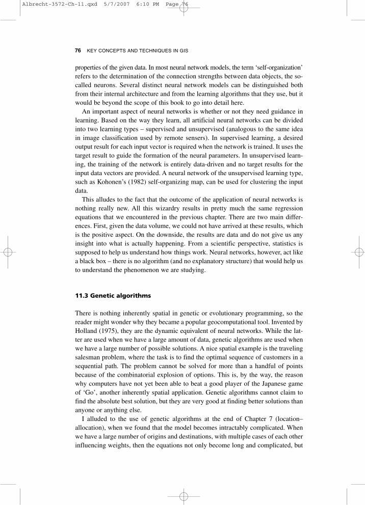
properties of the given data. In most neural network models, the term ‘self-organization’refers to the determination of the connection strengths between data objects, the so-called neurons. Several distinct neural network models can be distinguished bothfrom their internal architecture and from the learning algorithms that they use, but itwould be beyond the scope of this book to go into detail here.
An important aspect of neural networks is whether or not they need guidance inlearning. Based on the way they learn, all artificial neural networks can be dividedinto two learning types – supervised and unsupervised (analogous to the same ideain image classification used by remote sensers). In supervised learning, a desiredoutput result for each input vector is required when the network is trained. It uses thetarget result to guide the formation of the neural parameters. In unsupervised learn-ing, the training of the network is entirely data-driven and no target results for theinput data vectors are provided. A neural network of the unsupervised learning type,such as Kohonen’s (1982) self-organizing map, can be used for clustering the inputdata.
This alludes to the fact that the outcome of the application of neural networks isnothing really new. All this wizardry results in pretty much the same regressionequations that we encountered in the previous chapter. There are two main differ-ences. First, given the data volume, we could not have arrived at these results, whichis the positive aspect. On the downside, the results are data and do not give us anyinsight into what is actually happening. From a scientific perspective, statistics issupposed to help us understand how things work. Neural networks, however, act likea black box – there is no algorithm (and no explanatory structure) that would help usto understand the phenomenon we are studying.
11.3 Genetic algorithms
There is nothing inherently spatial in genetic or evolutionary programming, so thereader might wonder why they became a popular geocomputational tool. Invented byHolland (1975), they are the dynamic equivalent of neural networks. While the lat-ter are used when we have a large amount of data, genetic algorithms are used whenwe have a large number of possible solutions. A nice spatial example is the travelingsalesman problem, where the task is to find the optimal sequence of customers in asequential path. The problem cannot be solved for more than a handful of pointsbecause of the combinatorial explosion of options. This is, by the way, the reasonwhy computers have not yet been able to beat a good player of the Japanese gameof ‘Go’, another inherently spatial application. Genetic algorithms cannot claim tofind the absolute best solution, but they are very good at finding better solutions thananyone or anything else.
I alluded to the use of genetic algorithms at the end of Chapter 7 (location–allocation), when we found that the model becomes intractably complicated. Whenwe have a large number of origins and destinations, with multiple cases of each otherinfluencing weights, then the equations not only become long and complicated, but
76 KEY CONCEPTS AND TECHNIQUES IN GIS
Albrecht-3572-Ch-11.qxd 5/7/2007 6:10 PM Page 76

the possible solution space of varying parameters become as large as in our travelingsalesman problem, as depicted in Figure 65. Who would venture a guess, which partof the equation should be tweaked to improve the result?
GEOCOMPUTATION 77
Figure 65 Genetic algorithms are mainly applied when the model becomes toocomplicated to be solved deterministically
Evolutionary programming starts by generating a population of purely randomexpression – that is, random model equations. These are evaluated in terms of afitness function. The best expressions are reused and sent to compete with a newgeneration of crossovers and slightly mutated versions of previously successfulexpressions. This process is repeated until no improvement is achieved. The terms‘crossover’ and ‘mutation’ are borrowed from their biological analogues and func-tions exactly the same way (see Figure 66). A crossover is a mixing of previouslysuccessful strategies, while a mutation is a slight alteration. Together with the bestmembers of a previous generation, these new entities have to prove themselves. Ifthey succeed (i.e., fare better in the evaluation of fitness for a particular goal), thenthey are allowed to stay for the next round.
Evolutionary techniques have not yet made it into commercially available GISpackages, but public domain versions of linkages are available. The interested readermay want to search www.sourceforge.net for a combination of the terms genetic andGIS.
11.4 Cellular automata
CA are a modeling framework for spatially continuous phenomena (Langton 1986),such as landscape processes or urban sprawl (Haff 2001; Box 2002; Silva and Clarke2002). They are simple models used to represent the diffusion of things such as matter,information or energy, over a spatial structure. In its most simple form, a CA is
Albrecht-3572-Ch-11.qxd 5/7/2007 6:10 PM Page 77
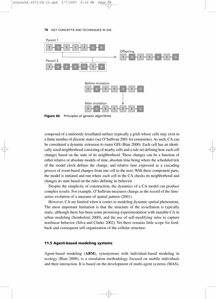
composed of a uniformly tessellated surface (typically a grid) whose cells may exist ina finite number of discrete states (see O’Sullivan 2001 for extensions). As such, CA canbe considered a dynamic extension to raster GIS (Bian 2000). Each cell has an identi-cally sized neighborhood consisting of nearby cells and a rule set defining how each cellchanges based on the state of its neighborhood. These changes can be a function ofeither relative or absolute models of time, absolute time being where the scheduled tickof the model clock defines the change, and relative time expressed as a cascadingprocess of event-based changes from one cell to the next. With these component parts,the model is initiated and run where each cell in the CA checks its neighborhood andchanges its state based on the rules defining its behavior.
Despite the simplicity of construction, the dynamics of a CA model can producecomplex results. For example, O’Sullivan measures change as the record of the time-series evolution of a measure of spatial pattern (2001).
However, CA are limited when it comes to modeling dynamic spatial phenomena.The most important limitation is that the structure of the tessellation is typicallystatic, although there has been some promising experimentation with mutable CA inurban modeling (Semboloni 2000), and the use of self-modifying rules to capturenonlinear behavior (Silva and Clarke 2002). Yet there remains little scope for feed-back and consequent self-organization of the cellular structure.
11.5 Agent-based modeling systems
Agent-based modeling (ABM), synonymous with individual-based modeling inecology (Bian 2000), is a simulation methodology focused on mobile individualsand their interaction. It is based on the development of multi-agent systems (MAS),
78 KEY CONCEPTS AND TECHNIQUES IN GIS
Parent 1
Parent 2
Offspring
Before mutation
After mutation
1 0 1 1 1 0 0
1 0 0 0 0 1 0
1 0 1 1 0 1 0
1 0 1 1 1 1 0
1 0 1 1 0 1 0
Figure 66 Principles of genetic algorithms
Albrecht-3572-Ch-11.qxd 5/7/2007 6:10 PM Page 78
which were created in the field of distributed artificial intelligence, a sub-field ofartificial intelligence (Gilbert and Terna 2000).
‘Agent’ is a generic term used for any constituent entity whose behavior we wishto model, and for its representation within the model. Agent-based models offer theability to capture the dynamic interactions of individuals and the context in whichthey occur. Agent-based models enable the creation of ‘artificial societies’ which canbe viewed as laboratories in which to conduct experiments (Epstein and Axtell1996). Agents are defined, placed in an environment and given a set of bounded rulesof behavior. The goal is to observe how interactions among individualsproduce the collective behaviors that are being studied.
An agent-based simulation implemented in the framework of a computationallaboratory offers the following advantages (Epstein and Axtell 1996; Gilbert andTerna 2000). First, agent-based models allow heterogeneity among individuals thatmore closely approximates the variety found in life. Second, the agents and the land-scape can be held constant or systematically varied in order to provide a level of con-trol impossible to attain using traditional social science methods. Third, thecombination of heterogeneous agents and control enables the researcher to conducta variety of experiments, using different conditions or applying various preventionscenarios and then evaluating outcomes for minimal cost compared to experimentsin the real world. Using simulations allows us to repeat experiments under controlledconditions and to compress spatio-temporal scales, so we are no longer limited toobserving just a few outcomes that happen to be presented by the real world. In addi-tion, we are able to explore, evaluate and refine alternative scenarios and plans forremediation safely and at reasonable costs and risks.
The observables or attributes of an agent (including spatial location) are meas-urable characteristics of the agent that change over time (Parunak et al. 1998).These observables describe the state of the system at any one time and are the pri-mary output of an ABM. ABMs develop histories of system states, where, as withtemporal extensions to GIS, change is handled by storing the system state at eachtime or by storing vectors of events for each agent; that is, an agent logs each newstate it enters. The focus of ABM is to understand the emergent outcome of eachmodel, where emergent ‘denotes the stable macroscopic patterns arising fromthe local interactions of agents’ (Epstein and Axtell 1996, p. 35). In terms ofspatial ABMs, this is the spatial pattern of observables (e.g. Parker and Meretskyforthcoming).
The primary distinction between CA and ABM is the conceptual primitive used torepresent phenomena. In CA, this primitive is a static cell or pixel, a collection ofwhich composes a layer of cells. Its dynamics involve each cell transferring infor-mation to its neighboring cells. An ABM, in contrast, is composed of distinguishableobjects, the same geometric primitives of point, line or polygon data models foundin GIS. Agent-based modeling enables the dynamic, situation-based decisions ofindividuals to drive emerging macro-level patterns of the phenomenon under studyand is indispensable to the modeling of individual-level decision-making.Furthermore, an agent has the added advantage of being mobile.
GEOCOMPUTATION 79
Albrecht-3572-Ch-11.qxd 5/7/2007 6:10 PM Page 79

There has been interest in intelligent software agents in GIScience in a varietyof contexts. In particular, agents have been employed in geographic simulationmodeling of a variety of phenomena, including simulation of land-use/cover change(Manson 2002; Parker et al. 2003), wayfinding (Raubal 2001) and social simulations(Gilbert and Doran 1994; Epstein and Axtell 1996; Gilbert and Troitzsch 1999;Conte et al. 2001). Only limited integration of GIS and agent-based models tosimulate social phenomena has been achieved (Gimblett 2002). Agent-based simu-lation models are particularly promising for urban applications (Batty 2001;Benenson et al. 2002; Deadman and Gimblett 1994; Dean et al. 2000; Westerveltand Hopkins 1999).
80 KEY CONCEPTS AND TECHNIQUES IN GIS
Albrecht-3572-Ch-11.qxd 5/7/2007 6:10 PM Page 80
Many of the geocomputational techniques discussed in the Chapter 11 go beyond thescope of commercial GIS. That is partly because the tools are too complicated for amass market, and partly because the problems these tools are applied to are tooacademic. Before the reader starts to abandon the concepts and techniques towardsthe end of this book as belonging into the ivory tower, I hasten to outline, with thisfinal chapter, why the research frontier is GIScience is important to the general pub-lic. This chapter could be read as ‘all the things you cannot (yet) do with GIS’.
Based on the last few chapters, the limitations of GIS should now be obvious. Inmost general terms, they can be described as the lack of currently easily availablesoftware to deal (a) with true 3-D, (b) with spatial processes, and (c) with qualitativedata. Interestingly, (a) does not seem to pose a significant problem in the real world.As discussed in Chapter 9, true 3-D GIS have been developed for mineral resourcesapplications (and arguably but not easily proven for military applications).
There are two distinct directions into which 3-D applications are moving. Basedon market demand and increased graphics capabilities of modern hardware, 3-Dvisualization is becoming commonplace. It comes in the form of spherical represen-tations of the globe, oblique scene rendering, fly-throughs, and even photographictextures of extruded buildings. For analytical purposes the development of true 3-Ddata structures is more interesting. There is an official standard in the form of thegeographic markup language (GML v3), a pseudo standard in the form of U3D(ECMA 2006), which now that it is supported in the latest versions of general-purpose document viewing software (Acrobat 8) achieves wide market penetration,and terrain models that mix and match all three forms of 3-D data: TINs, DEMs andextruded vector data. We hence now finally have the data structures to support real3-D analysis, and it is only a matter of time until the analysis methods will followsuit. One early example has been presented by Mennis et al. (2005) in the form of amultidimensional map algebra. The development of semantics for 3-D data thathelps us to distinguish buildings from each other by more than just their geometry ispart of the CityGML initiative (CityGML 2005).
The incorporation of qualitative data, and even more problematic, qualitativespatial relationships, has not progressed much in the past ten years. The emphasis inthat research area has shifted towards the development of spatial ontologies in sup-port of the semantic web, an intelligent classification of web-based data resourcesand already alluded to with respect to CityGML.
This leaves us the most promising area for new developments in GIScience – therealm of spatial process modeling. Cellular automata (CA) and agent-based models
12 EPILOGUE: FOUR-DIMENSIONAL MODELING
Albrecht-3572-Ch-12.qxd 5/7/2007 6:10 PM Page 81
(ABM) (Epstein and Axtell 1996; Gilbert and Terna 1999) were introduced inChapter 11. They become even more interesting when they are run on richly struc-tured landscapes. These bottom-up models focus on studying the emergent proper-ties of systems by starting with individual-level interactions. They both model thesame notion of underlying absolute space and utilize the same types of time, fallinginto what Zeigler terms discrete time or discrete event systems, depending on themodeling approach taken (Zeigler et al. 2000). The development of object-orientedsoftware design has enabled scientists to develop models that realistically reflect theobjects and relationships found in the real world (Gilbert and Terna 1999). And froma practical perspective, it allows software engineers to link GIS objects with ABMobjects, as for instance in the AgentAnalyst extension that has been developed as apublic domain project.
On a more traditional side, especially environmental scientists (hydrologists, ani-mal ecologists etc.) have for quite a while and with some success tried to nudge GISto deal with time. As long as this is done within GIS, most attempts are based on mapalgebra. Some looping and conditional constructs, well-known from procedural pro-gramming languages, allow for state-based changes of features. The change in alandscape is then the sum of the changes of the features that it consists of (Pullar2003). This, of course, does not capture transitions from one type of feature toanother, such as when a cliff erodes to become a beach. One step further goes thePCRaster system developed at the University of Utrecht (The Netherlands), whichaddresses the needs of geophysicists and hydrologists to include differential equa-tions in their GIS work.
Be it for lack of a commercial vendor or because a wider applicability has notbeen shown, many people interested in truly dynamic phenomena such as ground-water modeling (GMS, MODFLOW), wildfire spread (FARSITE), traffic conges-tions (EMME/2, WATSim) or weather forecasting (CALPUFF) prefer to link GISwith external software packages capable of dynamic modeling. What all of thesepackages lack (and why they link to GIS) is the notion of spatial differentiation.Space, and hence geography, is treated as a dependent variable if it is acknowledgedat all.
In addition to traditional forms of GIS process modeling or the linking of GISwith external dynamic modeling programs, there is a third, and so far not muchexplored option: truly spatio-temporal systems that have processes as their buildingblocks. Many of the processes that we study in geography and related disciplines arethe confluence of smaller scale (both spatial and temporal) processes. For instance,a housing boom can be the result of increased immigration, a disastrous hurricane,or the fact that other forms of capital investment are less lucrative. All of these arenot features in the traditional GIS sense but processes.
A logical question then is: What can we expect to see from this form of processmodeling in the near future? We will probably have a good number of process mod-els, all well-specified albeit in the beginning using different formalizations. Theresearch agenda therefore includes development of a uniform process descriptionlanguage, similar to what the unified modeling language (OMG 2005) does for
82 KEY CONCEPTS AND TECHNIQUES IN GIS
Albrecht-3572-Ch-12.qxd 5/7/2007 6:10 PM Page 82

structures (UML 2 allows for the representation of activities but falls short of theneeds of dynamic process modeling). Ideally, such a language would have theexpressiveness and ease of use of the web ontology language OWL (McGuinnessand van Harmelen 2004), while extending it to include rules and behavior. TheKepler system for scientific workflows is an early and still fairly primitive examplefor the kind of process libraries. The value of such process libraries has been recog-nized both in the business world, where process models are a well-establishedcomponent in operations research, and in the natural sciences (see, for example, theKepler system (http://keplerproject.org) that is part of the SEEK program heavilyfunded by NSF).
Linking these kinds of process model with 3-dimensional GIS models will be theultimate goal. Unfortunately, this book will be long out of print before we can expectsuch software systems in the hand of the reader.
EPILOGUE: FOUR-DIMENSIONAL MODELING 83
Albrecht-3572-Ch-12.qxd 5/7/2007 6:10 PM Page 83

ABM Agent-based modeling system – a simulation tool used to investigate theaggregate outcome of actions of individuals
Accuracy The difference between what is supposed to be encoded and whatactually is encoded
Address Short for street address, a spatial reference commonly used by postalservices and humans but not by GIS
Attribute The characteristic of a feature or location
AutoCAD™ Popular computer design program whose drawing exchange formathas become a de-facto standard for the exchange of geometric data
Autocorrelated Statistical fact underlying most geographic phenomena thatrenders traditional statistical techniques obsolete
Boolean logic Binary logic underlying most digital equipment; also commonlyused in GIS overlay operations
Buffer Result of a GIS operation determining the neighborhood of a feature
CA Cellular automata implement transition rules to mimic the evolution of anartificial landscape
CAD Computer-aided design – a type of software that processes geometries similarto GIS but at a larger scale, without geo-reference and less emphasis on the linkbetween geometries and attributes. A number of GISystems have been developedfrom CAD software
Centroid Middle-most (central) point of an area or region
Coordinate Location in a Cartesian or polar coordinate system
dBASE™ Originally a database program, it has become a de-facto standard for theexchange of attribute data
DEM Digital elevation model – a framework for recording spot elevations in araster layer
GLOSSARY
Albrecht-3572-Glossary.qxd 5/7/2007 6:10 PM Page 84

GLOSSARY 85
Digital number Attribute value of a cell in a raster image
Digitizing The act of transforming analogue data (such as a paper map) into digital data
Feature The object of interest in a GIS; it has to have a location and someattribute
Field view Represents space as a continuous surface of attributes
First Law An off remark in a 1970 article that became famous (... of Geography,because it indeed underlies everything geographical)
Focal function Neighborhood function in map algebra
FTP File transfer protocol – a network standard that is commonly used for thetransfer of large datasets
Fuzzy reasoning A form of multi-valued logic based on set theory that allows forreasoning with vague data and relationships
Geodemographics A spatial analysis of demographic data pioneered in marketingapplications
Geographic object See Feature
GeoTIFF TIFF format with a spatial reference
GIS Geographic Information System
GIScience Body of knowledge created by combining many of the motherdisciplines that are necessary for the successful development of GIS
GML Geographic markup language – an XML dialect for the exchange of databetween GISystems
GPS Global positioning system – an array of satellites that (given an appropriatereceiver) can help to determine one’s location on Earth
IDW Inverse distance weighting – a spatial interpolation method that incorporatesinformation from known points according to the inverse of their distance to theunknown point
ISO International Standards Organization, instrumental in setting many of thestandards (such as 19115) used for the processing of geographic information
Kriging Spatial interpolation method that uses weights based on the statisticalanalysis of covariances in a global point dataset
Albrecht-3572-Glossary.qxd 5/7/2007 6:10 PM Page 85
86 KEY CONCEPTS AND TECHNIQUES IN GIS
Lineage The history of a dataset – an important metadata item
Map algebra Extremely powerful rule set for combining raster layers
Map projection The application of mathematical formulas to transform sphericalcoordinates describing features on the surface of the Earth to Euclidean coordinatesused in most GIS
MapQuest® Company that pioneered the use of online mapping
MAUP Modifiable Area Unit Problem – arising from the attempt to combine setsof data that have been aggregated in different though overlapping spatial units
Metadata Literally data about data – important for archiving and re-use ofgeographic information
Neural network Computational technique that mimics brain functions to arrive atstatistical results
Object view Represents the features as discrete objects with well-definedboundaries in an empty space
Ontology Formal specification of the meaning of a datum
Overlay Quintessential GIS operation that determines spatial coincidences
PDF Portable document format – an open file format for the description ofdevice-independent documents
Pedologist One who studies soil science
Precision The amount of detail that can be discerned in geographic information
Projection See Map projection
Raster Spatial organization of data similar to an array or a spreadsheet; space iscompletely filled by the cells that make up the raster
Regional science Academic discipline at the intersection of economics andgeography that developed its own set of spatial analysis techniques
Remote sensing The technique (and science behind) gathering information fromobjects without touching them
Scanning An automated form of digitizing that results in raster data
Semantics The meaning of a datum
Albrecht-3572-Glossary.qxd 5/7/2007 6:10 PM Page 86
GLOSSARY 87
Shape measures Set of statistical measures to describe spatial configurations;originally developed in landscape ecology
Spatial reference Descriptor for a location on Earth
SQL Structured query language; a standard (with many variations) way of queryinga database
SVG Scalable vector graphics – an XML dialect for the description of vector data
Thiessen polygon For a point dataset, the area around one point that is closer tothis point than to any other point
TIFF Tagged image file format, an error-free storage format for raster data
TIN Triangulated irregular network, a representation of a surface derived fromirregularly spaced sample points
Topology Branch of mathematics that deals with qualitative spatial relations.Topological relationships are important for many GIS operations and have been usedas a check for the geometric consistency of a GIS database
UML Unified modeling language, an ISO standard for the specification of databaseschemas
Unix Family of multi-user operating systems
UTM Universal Transverse Mercator projection and coordinate system. Originallyused by the US armed forces, it is now common throughout the world for GISapplications covering larger areas
Vector GIS GIS that uses points, lines and polygons to represent geographic features
Web 2.0 A set of techniques associated with web technologies that enable users todevelop their own applications
XML Extended markup language, a superset of what many know as web descriptionlanguages such as HTML. XML is not meant to be read by humans but to facilitateautomated exchanges between computers
Albrecht-3572-Glossary.qxd 5/7/2007 6:10 PM Page 87

Alonso, W. (1978). A theory of movements. In Hansen, N.M. (ed.): Human SettlementSystems: International Perspectives on Structure, Change and Public Policy, pp. 197–211.Cambridge, MA: Ballinger Publishing.
Batty, M. (2001). Cellular dynamics: modelling urban growth as a spatial epidemic. InFischer, M. and Y. Leung (eds): GeoComputational Modelling: Techniques and Application,pp. 109–141. Berlin: Springer-Verlag.
Benenson, I., Omer, I. and Hatna, E. (2002). Entity-based modeling of urban residentialdynamics: the case of Yaffo, Tel Aviv. Environment and Planning B: Planning and Design,29, 491–512.
Bettinger, P. and Sessions, J. (2003). Spatial forest planning: to adopt, or not to adopt? Journalof Forestry, 101(2), 24.
Bian, L. (2000). Object-oriented representation for modelling objects in an aquatic environ-ment. International Journal of Geographic Information Science, 14, 603–623.
Box, P. (2002). Spatial units as agents: making the landscape an equal player in agent-basedsimulations. In Gimblett, H.R. (ed.): Integrating Geographic Information Systems andAgent-based Modeling Techniques for Simulating Social and Ecological Processes,pp. 59–82. New York: Oxford University Press.
Bryant, R. (2005). Assisted GPS: using cellular telephone networks for GPS anywhere. GPSWorld, May 2005, 40–46. Online article at www.gpsworld.com/gpsworld/content/printContentPopup.jsp?id=163593
Burrough, P.A. (1986). Principles of Geographic Information Systems. Oxford: OxfordUniversity Press.
Burrough, P.A. and Frank, A.U. (1996). Geographic Objects with Indeterminate Boundaries.London: Taylor & Francis.
Chrisman, N. (2002). Exploring Geographic Information Systems. New York: Wiley.CityGML (2005). Exchange and storage of virtual 3D city models. OGC discussion paper,
available online at https://portal.opengeospatial.org/files/?artifact_id=16675Conte, R., Edmonds, B., Moss, S. and Sawyer, K. (2001). Sociology and social theory in
agent-based social simulation: a symposium. Computational and MathematicalOrganization Theory, 7(3), 183–205.
Couclelis, H. (1982). Philosophy in the construction of geographic reality: some thoughtsupon the advent of the ‘qualitative revolution’ in human geography. In Gould, P. and Olsson,G. (eds): A Search for Common Ground, pp. 105–138. London: Pion.
Couclelis, H. (1992). People manipulate objects (but cultivate fields): beyond the raster–vector debate in GIS. In Theories and Methods of Spatio-Temporal Reasoning inGeographic Space, vol. 639. Berlin: York: Springer-Verlag.
Deadman, P. and Gimblett. H.R. (1994). The role of goal-oriented autonomous agents inmodeling people–environment interactions in forest recreation. Mathematical andComputer Modeling, 20(8), 121–133.
Dean, J.S., Gumerman, G.J., Epstein, J.M., Axtell, R.L., Swedlund, A.C., Parker, M.T. andMcCarroll, S. (2000). Understanding Anasazi cultural change through agent-based model-ing. In Kohler, T.A. and Gumerman, G.J. (eds): Dynamics in Human and Primate Societies,pp. 179–205. Oxford: Oxford University Press.
ECMA (2006). Universal 3D File Format, 3rd edn. ECMA International and EuropeanAssociation for Standardizing Information and Communication Systems, Geneva. Onlinedocument accessible at www.ecma-international.org/publications/files/ECMA-ST/ECMA-363.pdf
REFERENCES
Albrecht-3572-References.qxd 5/7/2007 6:09 PM Page 88
REFERENCES 89
Egenhofer, M. (1993). A model for detailed binary topological relationships. Geomatica,47(3/4), 261–273.
Epstein, J.M. and Axtell, R. (1996). Growing Artificial Societies: Social Science from theBottom Up. Cambridge, MA: MIT Press.
Gilbert, N. and Doran, J. (eds) (1994). Simulating Societies: The Computer Simulation ofSocial Phenomena. London: UCL Press.
Gilbert, N. and Troitzsch, K.G. (1999). Simulation for the Social Scientist. Buckingham: OpenUniversity Press.
Gilbert, N. and Terna, P. (2000). How to build and use agent-based models in social science.Mind & Society, 1, 57–72.
Gimblett, H.R. (ed.) (2002). Integrating Geographic Information Systems and Agent-basedModeling Techniques for Simulating Social and Ecological Processes [Sante Fe InstituteStudies in the Sciences of Complexity]. New York: Oxford University Press.
Gregory, I. (2003). A Place in History: A Guide to Using GIS in Historical Research. Oxford:Oxbow Books.
Haff, P.K. (2001). Waterbots. In Harmon, R.S. and Doe, W.W. (eds): Landscape Erosion andEvolution Modeling, pp. 239–275. New York: Kluwer.
Hamil, D. (2001). Your mission, should you choose to accept it: project management excel-lence. Online article at http://spatialnews.geocomm.com/features/mesa1/hamil1.pdf
Hebb, D.O. (1949). The Organization of Behavior: A Neuropsychological Theory. New York:Wiley.
Holland, J.H. (1975). Adaptation in Natural and Artificial Systems: An Introductory Analysiswith Applications to Biology, Control, and Artificial Intelligence. Ann Arbor: University ofMichigan Press.
Kirby, K. and Pazner, M. (1990). Graphic map algebra. In Brassel/Kishimoto (eds):Proceedings of the 4th International Symposium on Spatial Data Handling, vol. 1,pp. 413–422. Columbus, Ohio, USA: International Geographical Union (IGU),Commission on Geographic Information Systems.
Kohonen, T. (1982). Self-organized formation of topologically correct feature maps.Biological Cybernetics, 43, 59–69.
Langton, C. (1986). Studying artificial life with cellular automata. Physica D, 22, pp. 120–149.Maantay, J. and Ziegler, J. (2006). GIS for the Urban Environment. Redlands, CA: ESRI
Press.Manson, S.M. (2002). Integrated assessment and projection of land-use and land-cover
change in the Southern Yucatán Peninsular Region of Mexico. In Parker, D.C., Berger, T.and Manson, S.M. (eds): Agent-based Models of Land-Use and Land-Cover Change,pp. 56–59. Bloomington, IN: LUCC International Project Office.
McGuinness, D.L. and van Harmelen, F. (2004). OWL web ontology language overview:W3C recommendation 10 February 2004. Available at www.w3.org/TR/owl-features
Mennis, J., Leong, J. and Khanna, R. (2005). Multidimensional map algebra. In Proceedingsof the 8th International Conference on GeoComputation, 1–3 August, Ann Arbor, MI.Ypsilante, Michigan, USA: Institue for Geospatial Research & Education.
Mitchell, M.L. and Jolley, J.M. (2001). Research Design Explained, 4th edn. Pacific Grove,CA: Wadsworth.
OMG (2005). Introduction to PMG’s Unified Modeling Language. Needham, MA: ObjectManagement Group. Online document, accessible at www.omg.org/gettingstarted/what_is_uml.htm
O’Sullivan, D. (2001). Exploring spatial process dynamics using irregular cellular automatonmodels. Geographical Analysis, 33, 1–18.
Parker, D., and Meretsky, V. (2004). Measuring Pattern Outcomes in an Agent-Based Modelof Edge-effect Externalities using Spatial Metrics. Agriculture, Ecosystems, andEnvironment, 101: 233–250.
Parker, D.C., Manson, S.M., Janssen, M.A., Hoffmann, M.J. and Deadman, P. (2003). Multi-agent systems for the simulation of land-use and land-cover change: a review. Annals of theAssociation of American Geographers, pp. 314–337.
Parunak, H.V.D., Sauter, J. and Clark, S.J. (1998). Toward the specification and design ofindustrial synthetic ecosystems. In Singh, M.P., Rao, A. and Wooldridge, M.J. (eds):
Albrecht-3572-References.qxd 5/7/2007 6:09 PM Page 89
90 KEY CONCEPTS AND TECHNIQUES IN GIS
Intelligent Agents IV: Agent Theories, Architectures, and Languages [Lecture Notes inArtificial Intelligence 1365], pp. 45–59. Berlin: Springer. Available at www.altarum.net/~van/agentDesignMethod.pdf
Pullar, D. (2003). Simulation modelling applied to runoff modelling using MapScript. TGIS,7(2), 267–283.
Raubal, M. (2001). Ontology and epistemology for agent-based wayfinding simulation.International Journal of Geographical Information Science, 15(7), 653–665.
Reggiani, A. (2001). Spatial Economic Science: Frontiers in Theory and Methodology. Berlin:Springer-Verlag.
Semboloni, F. (2000). The growth of an urban cluster into a dynamic self-modifying spatialpattern. Environment and Planning B, 27, 549–564.
Silva, E.A. and Clarke, K.C. (2002). Calibration of the SLEUTH urban growth model forLisbon and Porto, Portugal. Computers, Environment and Urban Systems, 26, 525–552.
Tobler, W.R. (1970). A computer movie simulating urban growth in the Detroit Region.Economic Geography, 46, 234–240.
Tomlin, C.D. (1990). Geographic information systems and cartographic modeling.Englewood Cliffs, NJ: Prentice-Hall.
Wesseling, C. and van Deursen, W. (1995). A spatial modelling language for integratingdynamic environmental simulations in GIS. In Proceedings of the Joint EuropeanConference and Exhibition on Geographical Information, (JEC-GI), vol. 1, pp. 368–373.Lisbon, Portugal: European Unbrella Organisation for Geographic Information.
Westervelt, J.D. and Hopkins, L.D. (1999). Modeling mobile individuals in dynamic land-scapes. International Journal of Geographical Information Science, 13(3), 191–208.
Wilson, J.P. and Gallant, J.C. (2000). Terrain Analysis: Principles and Applications. NewYork: Wiley.
Zadeh, L. (1965). Fuzzy Logic and its Applications. New York: Academic Press.Zeigler, B.P., Praehofer, H. and Kim, T.G. (2000). Theory of Modeling and Simulation:
Integrating Discrete Event and Continuous Complex Dynamic Systems. San Diego:Academic Press.
Albrecht-3572-References.qxd 5/7/2007 6:09 PM Page 90