kevin merchant document

ITM UNIVERSE Signal & System

140953109008 EE A

Lab 1: Introduction to MATLAB

AIM: Introduction to MATLAB

INTRODUCTION:

MATLAB stands for Matrix Laboratory. MATLAB is a high-performance language for

technical computing. It integrates computation, visualization, and programming in an easy-to-

use environment where problems and solutions are expressed in familiar mathematical

notation. Typical uses include

Math and computation

Algorithm development

Data acquisition

Modelling, simulation, and prototyping

Data analysis, exploration, and visualization

Scientific and engineering graphics

Application development, including graphical user interface building.

The MATLAB System:

The MATLAB system consists of five main parts:

Development Environment. This is the set of tools and facilities that help you use

MATLAB functions and files. Many of these tools are graphical user interfaces. It

includes the MATLAB desktop and Command Window, a command history, an

editor and debugger, and browsers for viewing help, the workspace, files, and the

search path.

The MATLAB Mathematical Function Library. This is a vast collection of

computational algorithms ranging from elementary functions, like sum, sine, cosine,

and complex arithmetic, to more sophisticated functions like matrix inverse, matrix

eigen values, Bessel functions, and fast Fourier transforms.

The MATLAB Language. This is a high-level matrix/array language with control

flow statements, functions, data structures, input/output, and object-oriented

programming features. It allows both "programming in the small" to rapidly create

quick and dirty throw-away programs, and "programming in the large" to create large

and complex application programs.

Graphics. MATLAB has extensive facilities for displaying vectors and matrices as

graphs, as well as annotating and printing these graphs. It includes high-level

functions for two-dimensional and three-dimensional data visualization, image

processing, animation, and presentation graphics. It also includes low-level functions

that allow you to fully customize the appearance of graphics as well as to build

complete graphical user interfaces on your MATLAB applications.

The MATLAB Application Program Interface (API). This is a library that allows

you to write C and Fortran programs that interact with MATLAB. It includes facilities


140953109008 EE A

for calling routines from MATLAB (dynamic linking), calling MATLAB as a

computational engine, and for reading and writing MAT-files.

MATLAB Desktop:

When we start MATLAB, the MATLAB desktop appears, containing tools (graphical user

interfaces) for managing files, variables, and applications associated with MATLAB. The

following illustration shows the default desktop. You can customize the arrangement of tools

and documents to suit your needs.

MATLAB Windows:

1. MATLAB Desktop:

It consists of following sub windows.

a) Command Windows: This is the main window. It is characterized by the MATLAB

command prompt (>>).

b) Current Directory: This is where all your files from the current directory are listed. You

can do file navigation here.

c) Workspace: It lists all variables that you have generated so far and shows their types and

sizes.


140953109008 EE A

d) Command History: All commands typed on the MATLAB prompt in the command

window get recorded, even across multiple sessions.

2. Figure Window:

The output of all graphics command typed in the command window is flushed to the figure

window.

3. Editor Window:

This is where you can write edit, create and save your own programs in files called m files.

MATLAB on the Windows System:On the windows systems, MATLAB is started by

double clicking the MATLAB icon on the desktop or by selecting MATLAB from the start

menu.

The starting procedure takes the user to the command window where the command line is

indicated with '>>'.

Help and information on MATLAB commands can be found in several ways.

From the command line by using the ‘help <topic name>' command. From the separate Help window found under the Help menu.

Prototype M-Files:

When you use the mfile name option with load library, MATLAB generates an M-file called

a prototype file. This file can then be used on subsequent calls to load library in place of a header file.

Scripts:

When you invoke a script, MATLAB simply executes the commands found in the file.

Scripts can operate on existing data in the workspace, or they can create new data on which to operate. Although scripts do not return output arguments, any variables that they create remain in the workspace, to be used in subsequent computations. In addition, scripts can

produce graphical output using functions like plot.

Functions:

Return information about a function handle SyntaxS = functions(funhandle)

Description:

S = functions(funhandle) returns, in MATLAB structure S, the function name, type, filename,

and other information for the function handle stored in the variable funhandle.


140953109008 EE A

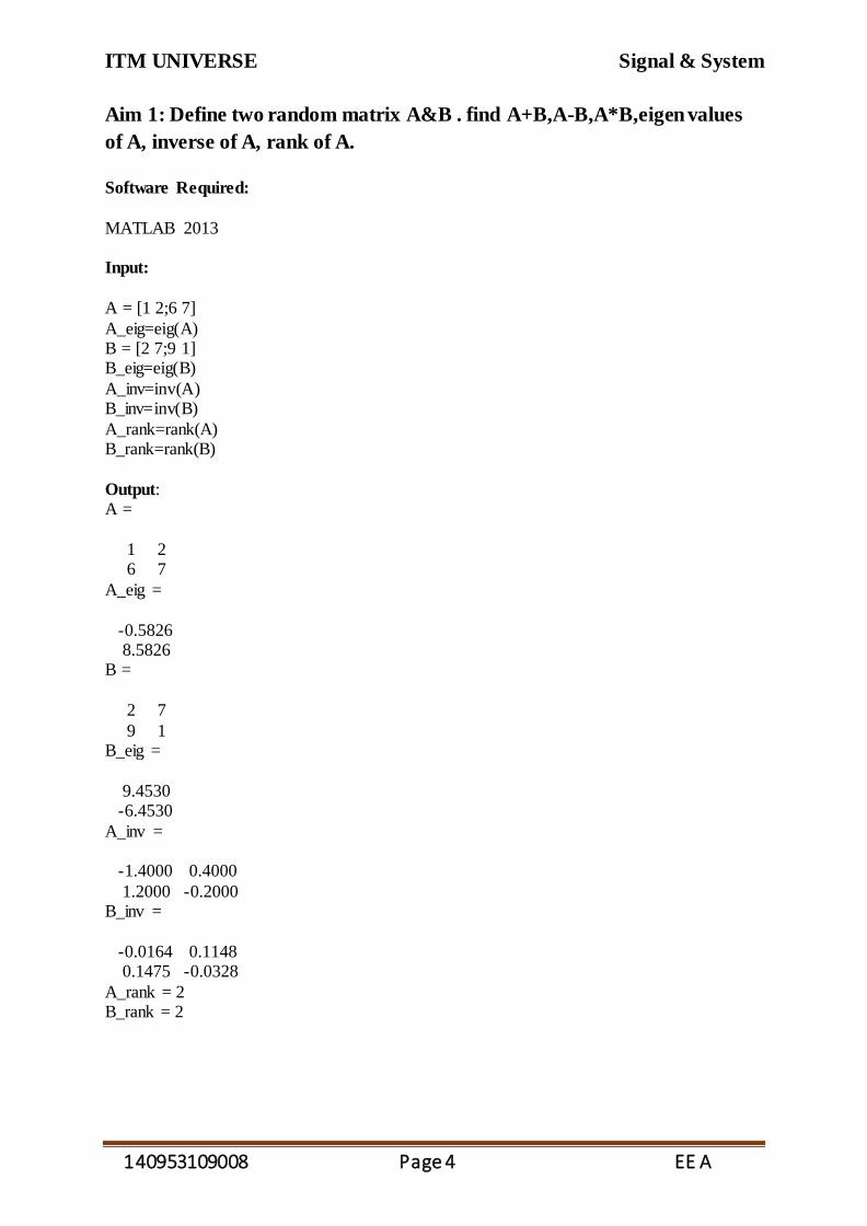
Aim 1: Define two random matrix A&B . find A+B,A-B,A*B,eigen values

of A, inverse of A, rank of A.

Software Required:

MATLAB 2013 Input:

A = [1 2;6 7]

A_eig=eig(A) B = [2 7;9 1] B_eig=eig(B)

A_inv=inv(A) B_inv=inv(B)

A_rank=rank(A) B_rank=rank(B)

Output: A =

1 2 6 7

A_eig =

-0.5826 8.5826 B =

2 7

9 1 B_eig =

9.4530 -6.4530

A_inv = -1.4000 0.4000

1.2000 -0.2000 B_inv =

-0.0164 0.1148 0.1475 -0.0328

A_rank = 2 B_rank = 2


140953109008 EE A

Aim 2: y=(x*2)+4*x+3 defined x from 0 to 200 in steps of 20.plot its discrete

samples.

Software Required:

MATLAB 2013

Input :

x=0:20:200

y=x.^2+4*x+3 stem(x,y);xlabel('x');ylabel('x^2+4*x+3');title('function');

output :

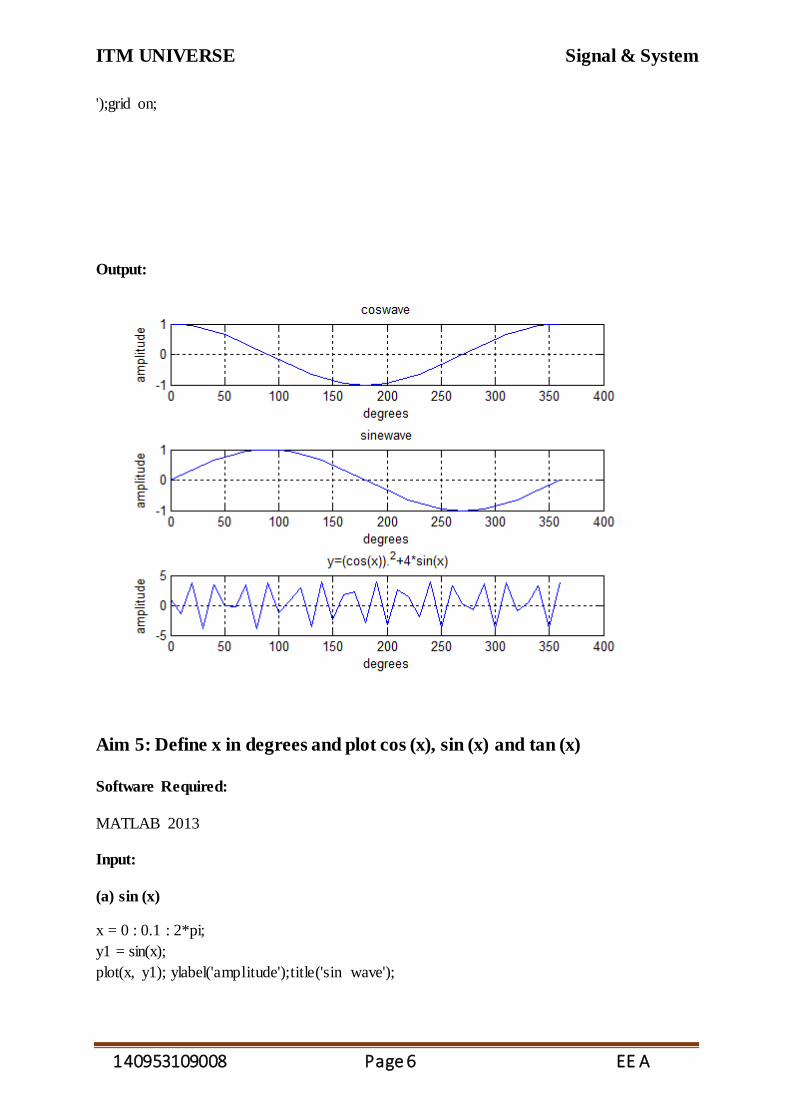
Aim3 : 0 to 360 steps of 10 y=(cos(x)).^2+4*sin(x).

Software Required:

MATLAB 2013

Input :

x=0:10:360

y=(cos(x)).^2+4*sin(x) subplot(3,1,1),plot(x,cosd(x));xlabel('degrees');ylabel('amplitude');title('coswave');grid on; subplot(3,1,2),plot(x,sind(x));xlabel('degrees');ylabel('amplitude');title('sinewave');grid on;

subplot(3,1,3),plot(x,y); xlabel('degrees');ylabel('amplitude');title(' y=(cos(x)).^2+4*sin(x)

0 20 40 60 80 100 120 140 160 180 2000

0.5

1

1.5

2

2.5

3

3.5

4

4.5x 10

4

x

x2+

4*x

+3

function


140953109008 EE A

');grid on;

Output:

Aim 5: Define x in degrees and plot cos (x), sin (x) and tan (x)

Software Required:

MATLAB 2013 Input:

(a) sin (x)

x = 0 : 0.1 : 2*pi;

y1 = sin(x);

plot(x, y1); ylabel('amplitude');title('sin wave');


140953109008 EE A

(b) cos (x)

x = 0 : 0.1 : 2*pi;

y2 = cos(x);

plot(x, y2) ; ylabel('amplitude');title('cos wave');

(c) tan (x)

x = 0 : 0.1 : 2*pi;

y3 = tan(x);

plot(x, y1) ; ylabel('amplitude');title('tan wave');

Output:

(a)

(b)


140953109008 EE A

(c)


140953109008 EE A

Conclusion:

After performing this experiment we studied about MATLAB and its basic operations and

functions.


140953109008 EE A

LAB. : 2 Signal Generation

Aim 1:Plot (a)sine wave and (b)cosine wave in continues time signal.

Software Required:

MATLAB 2013

Input:

(a) sin wave

f=50 Fs=1000; Ts=1/Fs

nts=0:Ts:1/f s=sin(2*pi*f*nts);

plot(nts,s);xlabel('time');ylabel('amplitude');title(‘sine wave’);grid on;

(b) cosine wave

f=50

Fs=1000 Ts=1/Fs nts=0:Ts:1/f

s=cos(2*pi*f*nts); plot(nts,s);xlabel('time');ylabel('amplitude');title('cos wave');grid on;


140953109008 EE A

output: (a)

(b)


140953109008 EE A

Aim 2:Plot (a)sine wave and (b)cosine wave in discrete time signal.

Software Required:

MATLAB 2013

Input:

(a)

f=50

Fs=input('sampling frequency'); Ts=1/Fs

n=0:Ts:Fs/f s=sin(2*pi*f*n*Ts); stem(n,s);xlabel('fre.');ylabel('amplitude');title('sin wave)');

(b) f=50

Fs=1000 Ts=1/Fs nts=0:Ts:1/f

s=cos(2*pi*f*nts); stem(nts,s);xlabel('fre.');ylabel('amplitude');title('cos wave');


140953109008 EE A

Output: (a) &(b) respectively

0 2 4 6 8 10 12 14 16 18 20-1

-0.8

-0.6

-0.4

-0.2

0

0.2

0.4

0.6

0.8

1

fre.

am

p.

sine wave

0 2 4 6 8 10 12 14 16 18 20-1

-0.8

-0.6

-0.4

-0.2

0

0.2

0.4

0.6

0.8

1

fre.

am

p.

cosine wave


140953109008 EE A

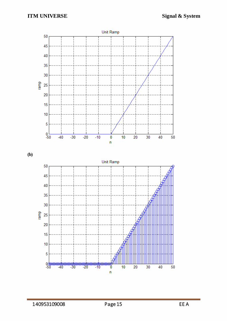
Aim3:Plot unit ramp function (Both in CT & DT domain).

Software Required:

MATLAB 2013

Input:

(a)

Fs=200 Ts=1/Fs

n=-50:1:50 [a,b]=size(n) for i=1:b

if n(i)>=0 ramp(i)=n(i)

else ramp(i)=0 end end

plot(n,ramp);xlabel('n');ylabel('ramp');title ('Unit_Ramp');grid on

(b)

Fs=200

Ts=1/Fs n=-50:1:50

[a,b]=size(n) for i=1:b if n(i)>=0

ramp(i)=n(i) else ramp(i)=0

end end stem(n,ramp);xlabel('n');ylabel('ramp');title ('Unit_Ramp');grid on

output:

(a)


140953109008 EE A

(b)


140953109008 EE A

Aim4: plot unit step function.(Both in CT & DT domain)

Software Required:

MATLAB 2013

Input:

(a)

Fs=200 Ts=1/Fs

nTs=-2:Ts:2 [a,b]=size(nTs) for i=1:b

if nTs(i)>0 step(i)=1

else step(i)=0 end end

plot(nTs,step);xlabel('nTs');ylabel('step');title ('unit step');grid on

(b)

Fs=200 Ts=1/Fs

nTs=-2:Ts:2 [a,b]=size(nTs)

for i=1:b if nTs(i)>0 step(i)=1

else step(i)=0 end

end stem(nTs,step);xlabel('nTs');ylabel('step');title ('unit_step');grid on

output:

(a)


140953109008 EE A

(b)


140953109008 EE A

Aim5 :plot delta function in (a) continuos and (b) descrete time signal.

Software Required:

MATLAB 2013

Input:

(a)

Fs=200 Ts=1/200

nTs=-0.2:Ts:0.2 [a,b]=size(nTs) for i=1:b

if nTs(i)==0 delta(i)=1

else delta(i)=0

end; end;

plot(nTs,delta);xlabel('nTs');ylabel('amplitude');title('delta continous');grid on; (b)

Fs=200 Ts=1/200

nTs=-0.2:Ts:0.2 [a,b]=size(nTs) for i=1:b

if nTs(i)==0 delta(i)=1

else delta(i)=0

end; end;

stem(nTs,delta);xlabel('nTs');ylabel('amplitude');title('Delta Discrete time');grid on;

output

(a)


140953109008 EE A

(b)

Aim 6: plot sinc function in (a)continous(b)descrete time signal.


140953109008 EE A

Software Required:

MATLAB 2013

Input:

(a)

f=50 Fs=2000

Ts=1/Fs nTs=-.5:Ts:.5 s=sin(2*pi*f*nTs);

sinc_s=s./(2*pi*f*nTs); plot(nTs,sinc_s);xlabel('time');ylabel('amplitude');title('sinc continuous signal');grid on;

(b) f=50 Fs=2000

Ts=1/Fs nTs=-.5:Ts:.5

s=sin(2*pi*f*nTs); sinc_s=s./(2*pi*f*nTs); stem(nTs,sinc_s);xlabel('time');ylabel('amplitude');title('sinc descrete signal');

Output:(a)

(b)


140953109008 EE A

CONCLUSION:

After performing this experiment we studied about different function and their waveform in

both continuous time and discrete time domain.


140953109008 EE A

LAB. : 3 Sampling Theorem

Aim 1 : Show effect of sampling effect of sampling frequency & prove

nyquist criteria for sampling.

Software Required:

MATLAB 2013

Input:

f=3

Fs1=1.5*f%Fs1<2*f nTs1=0:1/Fs1:2/f s=sin(2*pi*f*nTs1)

figure; plot(nTs1,s);hold on; stem(nTs1,s);hold off;xlabel('nTs');ylabel('Amplitude');title('Discrete

sine wave Fs<2Fm'); f=3

Fs2=2*f%Fs2=2*f nTs2=0:1/Fs2:2/f

s=sin(2*pi*f*nTs2) figure; plot(nTs2,s);hold on; stem(nTs2,s);hold off;xlabel('nTs');ylabel('Amplitude');title('Discrete

sine wave Fs=2Fm');

f=3 Fs3=5*f%Fs3>2*f nTs3=0:1/Fs3:2/f

s=sin(2*pi*f*nTs3) figure;

plot(nTs3,s);hold on; stem(nTs3,s);hold off;xlabel('nTs');ylabel('Amplitude');title('Discrete sine wave Fs>2Fm');


140953109008 EE A

output:


140953109008 EE A

Aim 2 : Add different harmonics of sin wave having tone frequency 50 hz.

Software Required:

MATLAB 2013

Input :

f=2;

fs1=25*f;

t1=0:1/fs1:1;

s1=sin(2*pi*f*t1)+sin(2*pi*2*f*t1)+sin(2*pi*3*f*t1)+sin(2*pi*4*f*t1)+sin(2*pi*5*f*t1);

figure;

plot(t1,s1);xlabel('time');ylabel('amplitude');title('HARMONICS');hold on;

stem(t1,s1);hold off;

Output :


140953109008 EE A

CONCLUSION:

After performing this practical we studied about sampling frequency, nyquist rate and

sampling theorem by plotting graph of sin wave.


140953109008 EE A

LAB. : 4 :SIGNAL OPERATIONS

Aim 1 : Perform the time shifting, amplitude scaling, folding operation on

discrete time signal.

Input :

%%%%%%%%% exp %%%%%%%%%

clc;

clearall; closeall;

t=15; x=exp(1:5); plot(x);

v=shift(x,3,t); f=fold(x);

s_f=amp_scaling(x,3);

%%%%%%%% fold %%%%%%%%%%

function v=fold(x) k=size(x,2);

v=[]; fori=k:-1:1; v=[v x(i)];

end end

%%%%%%%% shift %%%%%%%%%

function v=shift(s,n,t) if n>0 v=[zeros(1,n) s zeros(1,t-abs(n)-size(s,2))];

elseif n<0 v=[s zeros(1,t-size(s,2))];

else v=[s zeros(1,t-size(s,2))]; end

end end

%%%%%%% amp_scaling %%%%%%

function v= amp_scaling(s,scal_factor) v=s*scal_factor


140953109008 EE A

%%%%%% code %%%%%

clc;

clearall; closeall;

t=15; x=exp(1:5); plot(x);

v=shift(x,3,t); f=fold(x);

s_f=amp_scaling(x,3); figure; subplot(2,2,1);plot(x);xlabel('time');ylabel('amplitude');title('exponatial');

subplot(2,2,2);plot(v);xlabel('time');ylabel('amplitude');title('shifting'); subplot(2,2,3);plot(f);xlabel('time');ylabel('amplitude');title('folding');

subplot(2,2,4);plot(s_f);xlabel('time');ylabel('amplitude');title('scaling'); Output:

Conclusion:

We Performed the time shifting, amplitude scaling, folding operation on discrete time signal.


140953109008 EE A

LAB. : 5 Generation of Continuous Time Domain Signals

Aim 1 : Recording of own voice and displaying its discrete samples

Software Required:

MATLAB 2013

Input:

% Record your voice for 5 seconds.

recObj = audiorecorder;

disp('Start speaking.')

recordblocking(recObj, 5);

disp('End of Recording.');

% Play back the recording.

play(recObj);

% Store data in double-precision array.

myRecording = getaudiodata(recObj);

% Plot the waveform.

plot(myRecording);

Output: Voice is recorded for 5 sec and the graph of the voice signal is obtained.


140953109008 EE A

Aim 2 : Record and save voice file with .wav extension

Software Required:

MATLAB 2013

Input :

clc;

%input

Fs=8000;

ButtonName= questdlg('press start to record your sound',...

'record',...

'START','STOP','START' );

switch ButtonName,

case 'START'

x=wavrecord(60000,Fs);

msgbox('Now you can hear the recorded sound', 'play');

wavplay(10*x,Fs);

case 'STOP'

errordlg('you dont want to record??? ','???')

x=0;

end

wavwrite(x,Fs,'C:\Users\Arpit Patel\Desktop');

x

Output :

Voice is recorded by clicking start button and recording is stopped by clicking stop button

and then recording is saved in .wav extension.

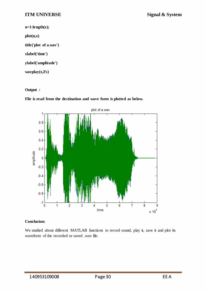
Aim 3 : Reading existing wave file

Software Required:

MATLAB 2013

Input :

%%%%%%%******program 5******%%%%%%

%processing of speech signal

[x,Fs]=wavread('C:\Users\Arpit Patel\Downloads\Music\a');


140953109008 EE A

n=1:length(x);

plot(n,x)

title('plot of a.wav')

xlabel('time')

ylabel('amplitude')

wavplay(x,Fs)

Output :

File is read from the destination and wave form is plotted as below.

Conclusion:

We studied about different MATLAB functions to record sound, play it, save it and plot its

waveform of the recorded or saved .wav file.


140953109008 EE A

LAB. : 6 Linearity

Aim 1 : Check linearity of the given function

Software Required:

MATLAB 2013

Input:

(a) y1(n)=2x(n)+3

x1=input(' enter input 1');


a1=input('weight of input 1');


Y11=2*(a1*x1+a2*x2)+3;

Y12=(2*(a1*x1)+3)+(2*(a2*x2)+3);

if Y11==Y12

disp('sys is linear ');

else

disp('sys is non-linear ');

end;

(b)





Y21=cos((a1*x1)+(a2*x2));

Y22=cos(a1*x1)+cos(a2*x2);

if Y21==Y22

disp('sys is linear ');

else

disp('sys is non-linear ');

end;


140953109008 EE A

output:

(a)

(b)

CONCLUSION:

We studied about linearity property and check linearity of the function using MATLAB.

kevin merchant document

Business

matlab functions

matlab desktop

matlab language

matlab windows

matlab system

matlab prompt

matlab applications

matlab command prompt