Kevin Cherry

Robert Firth

Manohar Karki

Bayesian Modeling of Dynamic Scenes for Object Detection

Accurate detection of moving objects within scenes with dynamic background, in scenarios where the camera is mostly stationary.

Problem Definition

Prerequisite for object tracking and recognition

Motivation

Methods that employ local (pixel-wise) models of intensity

Methods that have regional models of intensity

Previous Work– modelling intensity

Previous Work – Background Subtraction

Naïve approach: | framei – background | > thresholdBetter: | framei – μ | > kσ

Background – Bayes' theorem

𝑝 (ℒ|�̂� )=𝑝 ( �̂�|ℒ )𝑝 (ℒ )𝑝 (�̂� )

APPENDIX: EXAMPLE

Background – Minimum Cut

Background – Probability Density Estimator (parametric)

Background – Kernel Density Estimator(nonparametric)

𝐻=h2 𝐼

,…, �̂� h (𝑥 )=𝑛−1∑

𝑖=1

𝑛

𝐾 h (𝑥−𝑥 𝑖 )

Mean Squared Error:

Balloon Estimator:

Sample-point Estimator:

For computation reduction,

OR,

APPENDIX – Bandwidth Matrix Classes

Background - Bandwidth Estimation

𝐻=h2 𝐼 ,…,

𝑀𝑆𝐸 { 𝑓 𝐻 (𝑥 ) }=𝐸 {[ �̂� 𝐻 (𝑥 )− 𝑓 𝐻 (𝑥 ) ]2}

𝑓 (𝑥 )=1𝑛∑𝑖=1

𝑛

𝜑𝐻 (𝑥) (𝑥−𝑥 𝑖 )

𝑓 (𝑥 )=1𝑛∑𝑖=1

𝑛

𝜑𝐻 (𝑥 𝑖) (𝑥−𝑥 𝑖 )

Background: Markov Random Field

Guy flying kite. 15 consecutive frames merged using Photoshop.

Background– Temporal Persistence

Method Overview

Domain: (x, y) coordinates

Range: (r, g, b) color values at each (x, y) coordinate

Joint Domain-Range Representation:fR,G,B,X,Y (r, g, b, x, y)

Directly models dependencies between neighboring pixels

Joint Domain-Range Representation

[25520503050

]Examples:

[ 00255010

] [2552550100100

]

Modeling the Background

Background pixels: Y[0]= [15, 15, 15, 1, 1];Y[1]= [10,12,12.8,1,1];Y[2]= [ 16,1,2,1,1];Y[3]= [16, 10, 13, 1, 1];

Bandwidthmatrix H:16 0 0 0 0 0 16 0 0 0 0 0 16 0 0 0 0 0 31 0 0 0 0 0 21

Inverse of H:0.063 0 0 0 0 0 0.063 0 0 0 0 0 0.063 0 0 0 0 0 0.032 0 0 0 0 0 0.048

|H| = 2666495|H|-1/2 = 0.00061239

x = [16, 14, 15, 2, 1];

d = x – y[0] = [16-15,14-15,15-15,2-1,1-1] = [1,-1,0,1,0]dTH-1d= 0.1573ΦH = 0.00061239 * (2π)-5/2 * exp(-1/2 * 0.1573) = 5.72 x 10-6

P(x | ψb) = 4-1* (5.72 x 10-6 + 1.32 x 10-6 + 1.58 x 10-10+ 3.26 x 10-6) = 2.57 x 10-6

𝜑𝐻 (𝑥 )=|𝐻|− 1/2𝜑 (𝐻 −1/2𝑥 )𝑃 (𝑥|𝜓𝑏)=𝑛−1∑𝑖=1

𝑛

𝜑𝐻 (𝑥− 𝑦 𝑖 )

𝜑𝐻( 𝒩) (𝑥 )=|𝐻|− 1/2 (2𝜋 )−𝑑 /2 exp (− 12 𝑥𝑇𝐻−1𝑥 )

Method Overview

Foreground Probability:

Foreground Modeling

𝑃 (𝑥|𝜓 𝑓 )=𝛼𝛾+(1−𝛼 )𝑚−1∑𝑖=1

𝑚

𝜑𝐻 (𝑥− 𝑧𝑖 )

Foreground likelihood function

Foreground Modeling

Foreground pixels: y[0]= [15, 15, 15, 1, 1];Y[1]= [10,12,12.8,1,1];Y[2]= [ 16,1,2,1,1];Y[3]= [16, 10, 13, 1, 1];

Bandwidthmatrix H:16 0 0 0 0 0 16 0 0 0 0 0 16 0 0 0 0 0 31 0 0 0 0 0 21

Inverse of H:0.063 0 0 0 0 0 0.063 0 0 0 0 0 0.063 0 0 0 0 0 0.032 0 0 0 0 0 0.048

|H| = 2666495 |H|-1/2 = 0.00061239

x = [16, 14, 15, 2, 1];

d = x – y[0] = [16-15,14-15,15-15,2-1,1-1] = [1,-1,0,1,0]dTH-1d= 0.1573ΦH = 0.00061239 * (2π)-5/2 * exp(-1/2 * 0.1573) = 6.188 x 10-6

P(x | ψf) = (0.01 * (16*16*16*31*21)-1) + (1-0.01) * (4-1 * 2.57 x 10-

6)

Foreground Probability: 𝑃 (𝑥|𝜓 𝑓 )=𝛼𝛾+(1−𝛼 )𝑚−1∑𝑖=1

𝑚

𝜑𝐻 (𝑥− 𝑧𝑖 )

Method Overview

Likelihood Ratio Classifier

𝜏=−𝑙𝑛𝑃 (𝑥|𝜓𝑏)𝑃 (𝑥|𝜓 𝑓 )

𝛿 (𝑥 )={ −∧1 , 𝑖𝑓 𝜏>𝜅¿1 , h𝑜𝑡 𝑒𝑟𝑤𝑖𝑠𝑒

Spatial Context

4 Neighborhood Clique

Likelihood Function

𝑙 ( �̂�|ℒ )=∏𝑖=1

𝑝

𝑓 (𝑥 𝑖|ℓ𝑖 )=∏𝑖=1

𝑝

𝑓 (𝑥𝑖|𝜓 𝑓 )ℓ𝑖 𝑓 (𝑥𝑖|𝜓𝑏)1−ℓ 𝑖

ℒ={ 𝑓𝑜𝑟𝑒𝑔𝑟𝑜𝑢𝑛𝑑 ,𝑏𝑎𝑐𝑘𝑔𝑟𝑜𝑢𝑛𝑑 }

Posterior

𝑝 (ℒ|�̂� )=𝑝 ( �̂�|ℒ )𝑝 (ℒ )𝑝 (�̂� )

¿  (∏𝑖=1

𝑝

𝑓 (𝑥 𝑖|𝜓 𝑓 )ℓ 𝑖 𝑓 (𝑥 𝑖|𝜓𝑏)1−ℓ 𝑖)  𝑝 (ℒ )

𝑝 (�̂� )

𝑝 (ℒ )∝𝑒𝑥𝑝(∑𝑖=1

𝑝

∑𝑗=1

𝑝

𝜆 (ℓ𝑖 ℓ 𝑗+(1−ℓ𝑖 ) (1−ℓ 𝑗 ) ))

Log Posterior𝑝 (ℒ|�̂� )=𝑝 ( �̂�|ℒ )𝑝 (ℒ )

𝑝 (�̂� ) ¿  (∏𝑖=1

𝑝

𝑓 (𝑥 𝑖|𝜓 𝑓 )ℓ 𝑖 𝑓 (𝑥 𝑖|𝜓𝑏)1− ℓ 𝑖)𝑒𝑥𝑝(∑𝑖=1

𝑝

∑𝑗=1

𝑝

𝜆 (ℓ𝑖 ℓ 𝑗+(1−ℓ𝑖 ) (1−ℓ 𝑗 ) ))𝑝 (�̂� )

≈ (∏𝑖=1

𝑝

𝑓 (𝑥 𝑖|𝜓 𝑓 )ℓ 𝑖 𝑓 (𝑥 𝑖|𝜓𝑏)1−ℓ𝑖)𝑒𝑥𝑝(∑𝑖=1

𝑝

∑𝑗=1

𝑝

𝜆 (ℓ𝑖ℓ 𝑗+(1−ℓ𝑖 ) (1−ℓ 𝑗 ) ))

≈ (∏𝑖=1

𝑝

𝑓 (𝑥 𝑖|𝜓 𝑓 )ℓ 𝑖 𝑓 (𝑥 𝑖|𝜓𝑏)1− ℓ𝑖)+∑𝑖=1

𝑝

∑𝑗=1

𝑝

𝜆 (ℓ𝑖ℓ 𝑗+ (1−ℓ 𝑖 ) (1−ℓ 𝑗 ))

𝑙𝑛

≈∑𝑖=1

𝑝

𝑙𝑛( 𝑓 (𝑥𝑖|𝜓 𝑓 )𝑓 (𝑥𝑖|𝜓𝑏)

 )ℓ 𝑖  +∑𝑖=1𝑝

∑𝑗=1

𝑝

𝜆 (ℓ𝑖ℓ 𝑗+(1−ℓ𝑖 ) (1−ℓ 𝑗 ) )

Log Posterior

𝐿 (ℒ|�̂� )=∑𝑖=1

𝑝

𝑙𝑛( 𝑓 (𝑥 𝑖|𝜓 𝑓 )𝑓 (𝑥𝑖|𝜓𝑏 )

 )ℓ 𝑖  +∑𝑖=1𝑝

∑𝑗=1

𝑝

𝜆(ℓ 𝑖ℓ 𝑗+ (1−ℓ 𝑖 ) (1−ℓ 𝑗 ))

Method Overview

Optimization: Graph Construction

2

1 5

4

3S T

τ2 = 0.5

τ1 = 0.2

-τ3 = 0.07

-τ4 = 0.01

-τ5 = 0.1

1

1

1

1

1 1

1 1

1

11

τ1 = 0.20τ2 = 0.50τ3 = -0.07τ4 = -0.01τ5 = -0.10

λ = 1

0.50

0.20

-0.07

-0.10

-0.01

Log Ratio Classifier for 4-Neighborhood

Create a weighted graph G = {V, E}, where V = {v1, v2, v2, v4, v5, s, t}, where s is the source and t is the sink.

If τi > 0, connect s (source) to v i with weigh τi.Else, connect vi to t (sink) with weight -τi.

Next, add w(i, j) = λ if vi and vj are neighbors.

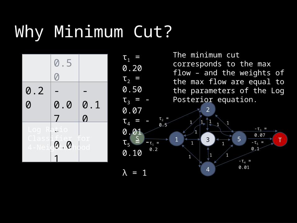
Why Minimum Cut?

2

1 5

4

3S T

τ2 = 0.5

τ1 = 0.2

-τ3 = 0.07

-τ4 = 0.01

-τ5 = 0.1

1

1

1

1

1 1

1 1

1

11

τ1 = 0.20τ2 = 0.50τ3 = -0.07τ4 = -0.01τ5 = -0.10

λ = 1

0.50

0.20

-0.07

-0.10

-0.01

Log Ratio Classifier for 4-Neighborhood

𝐿 (ℒ|�̂� )=∑𝑖=1

𝑝

𝑙𝑛( 𝑓 (𝑥 𝑖|𝜓 𝑓 )𝑓 (𝑥𝑖|𝜓𝑏 )

 )ℓ 𝑖  +∑𝑖=1𝑝

∑𝑗=1

𝑝

𝜆(ℓ 𝑖ℓ 𝑗+ (1−ℓ 𝑖 ) (1−ℓ 𝑗 ))

The minimum cut corresponds to the max flow – and the weights of the max flow are equal to the parameters of the Log Posterior equation.

Method Overview

Model Update

T = 23

T = 24

T = 25

T = 26

T = 27

T = 28

T = 29

T = next

ρb = 6

T = 26

T = 27

T = 28

T = 29

T = next

ρf = 3

DEMO

All tests run on a 3.06 GHz Intel Pentium 4 with 1 GB RAM.

Video sequences used a 240x360 resolution (0.08 megapixels).

Bandwidth matrix H parameterized as a diagonal matrix with three equal variances for the range and two for the domain, with hr = 16 and hd = 25.

Experimental Setup

Results

Results

Results

Mixture of Gaussians vs. Nonparametric

Object Level Detection Rates

Precision vs. Recall

❑❑

Precision Recall

Pixel-level detection recall and precision

Using the Mixture of Gaussians

Precision Recall

Uses a nonparametric kernel density estimator, which experimentally performs much better than a mixture of Gaussians estimator.

Innovations include using the joint domain-range representation, which allows us to easily incorporate spatial distribution into the decision process.

Also uses temporal persistence as a criterion for detection without feedback from higher level modules.

All likelihoods calculated are used in a MAP-MRF framework to find an optimal global inference of the solution based on local information.

Discussion

Weaknesses

Image stabilization – this algorithm only works for nominal camera motion

Variant to frame rates, extremely fast moving and slow moving objects.

Illumination Invariant.

Future Work

Turlach, Berwin. “Bandwidth Selection in Kernel Density Estimation”.

Dr. Gunturk's EE7750 Slides for Parameter Estimation

http://vision.eecs.ucf.edu/projects/Detecting%20and%20Segmenting%20Humans%20in%20Crowded%20Scenes/detection_examples.jpg

http://www.cs.ucf.edu/~sali/Projects/CoTrain/TitleImage.jpg

http://www.philender.com/courses/multivariate/notes2/er9.gif

http://math.bu.edu/people/sray/mat3.gif

References

APPENDIX– Mixture of Gaussians

APPENDIX– Mixture of Gaussians

APPENDIX – Bandwidth Matrix Classes

Spositive scalar

times the identity matrix

Ddiagonal matrix

with positive entries on the main diagonal

Fsymmetric

positive definite matrix

APPENDIX– Proper Kernel for KDE

Given:

• A doctor knows that meningitis causes stiff neck 50% of the time• Prior probability of any patient having meningitis is 1/50,000• Prior probability of any patient having stiff neck is 1/20

If a patient has stiff neck, what’s the probability he/she has meningitis?

APPENDIX : Example of Bayes Theorem

0002.020/1

50000/15.0

)(

)()|()|(

SP

MPMSPSMP