kernels for one-class nearest neighbour classification and comparison of...
TRANSCRIPT

Kernels for One-Class Nearest Neighbour Classification and Comparison of Chemical
Spectral Data
Shehroz Saeed Khan
College of Engineering and Informatics,
National University of Ireland, Galway,
Republic of Ireland
A thesis submitted in partial fulfilment of
the requirements for the degree of
Master of Science in
Applied Computing and Information Technology
May 2010
Research Supervisor: Dr. Michael G. Madden
Research Director: Professor Gerard J. Lyons

i
Dedicated to
my
beloved mother, Zarina Khan
&
sweet daughter, Aliza

i
Table of Contents
TABLE OF CONTENTS ...................................................................................................................... I
ACKNOWLEDGMENTS .................................................................................................................... V
LIST OF FIGURES ........................................................................................................................... VII
LIST OF TABLES ............................................................................................................................... IX
ABSTRACT .......................................................................................................................................... X
CHAPTER 1 ......................................................................................................................................... 1
ONE-CLASS CLASSIFICATION ....................................................................................................... 1
1.1. Introduction to One-class Classification ............................................................................................. 1
1.2. One-class Classification Vs Multi Class Classification .......................................................................... 2
1.3. Measuring Classification Performance of One-class Classifiers ........................................................... 3
1.4. Motivation and Problem Formulation ................................................................................................ 4
1.5. Overview of Thesis ............................................................................................................................. 5
1.6. Publications Resulting from the Thesis ............................................................................................... 6
CHAPTER 2 ......................................................................................................................................... 7
REVIEW: ONE-CLASS CLASSIFICATION AND ITS APPLICATIONS .................................... 7
2.1. Related Review Work in OCC ............................................................................................................. 7
2.2. Proposed Taxonomy .......................................................................................................................... 8
2.3. Category 1: Availability of Training Data ............................................................................................ 9

ii
2.4. Category 2: Algorithms Used ............................................................................................................ 11
2.4.1. Support Vector Machines .................................................................................................................. 11
2.4.2. One-class Support Vector Machine (OSVM) ...................................................................................... 13
2.4.3. One-Class Classifiers other than OSVMs............................................................................................ 20
2.4.3.1. One-Class Classifier Ensembles ..................................................................................................... 20
2.4.3.2. Neural Networks ........................................................................................................................... 22
2.4.3.3. Decision Trees ............................................................................................................................... 24
2.4.3.4. Other Methods ............................................................................................................................. 24
2.5. Category 3: Application Domain Applied .......................................................................................... 28
2.5.1. Text / Document Classification .......................................................................................................... 28
2.5.2. Other Application Domain ................................................................................................................. 35
2.6. Open Research Questions in OCC ..................................................................................................... 36
CHAPTER 3 ....................................................................................................................................... 38
SPECTRAL DATA, SIMILARITY METRICS AND LIBRARY SEARCH ................................. 38
3.1. Raman Spectroscopy ........................................................................................................................ 38
3.2. Some Definitions .............................................................................................................................. 40
3.2.1. Similarity ............................................................................................................................................ 40
3.2.2. Dissimilarity ....................................................................................................................................... 41
3.2.3. Comparison........................................................................................................................................ 41
3.2.4. Search ................................................................................................................................................ 41
3.2.5. Spectral Library .................................................................................................................................. 41
3.3. Spectral Data Pre-processing ............................................................................................................ 41
3.3.1. Normalization .................................................................................................................................... 42
3.3.2. Baseline Correction ........................................................................................................................... 43
3.4. Standard Spectral Search and Comparison Methods ........................................................................ 43
3.4.1. Euclidean Distance ............................................................................................................................. 44

iii
3.4.2. Pearson Correlation Coefficient ........................................................................................................ 44
3.4.3. First Derivative Correlation................................................................................................................ 44
3.4.4. Absolute Value Search ....................................................................................................................... 45
3.4.5. Citiblock ............................................................................................................................................. 45
3.4.6. Least Square Search ........................................................................................................................... 45
3.4.7. Peak Matching Method ..................................................................................................................... 46
3.4.8. Dot Product Metric ............................................................................................................................ 46
3.5. More Recent / Non-Standard Spectral Search and Comparison Methods ........................................ 46
3.5.1. Match Probability .............................................................................................................................. 47
3.5.2. Nonlinear Spectral Similarity Measure .............................................................................................. 48
3.5.3. A Spectral Similarity Measure using Bayesian Statistics .................................................................... 48
3.6. Spectral Similarity Methods Specific for Spectral Data ..................................................................... 49
3.6.1. Spectral Linear Kernel ........................................................................................................................ 49
3.6.2. Weighted Spectral Linear Kernel ....................................................................................................... 49
3.7. A New Modified Euclidean Spectral Similarity Metric ...................................................................... 51
3.8. Comparative Analysis of Spectral Search Methods ........................................................................... 54
3.8.1. Description of the Dataset ................................................................................................................. 54
3.8.2. Data Pre-processing ........................................................................................................................... 56
3.8.3. Methodology for Measuring Search Performance ............................................................................ 56
3.8.4. Testing Strategy ................................................................................................................................. 57
3.8.5. Spectral Search Algorithms ................................................................................................................ 58
3.9. Evaluation Relative to Standard Algorithms ..................................................................................... 59
3.9.1. Dichloromethane ............................................................................................................................... 59
3.9.2. Trichloroethane ................................................................................................................................. 61
3.9.3. Chloroform ........................................................................................................................................ 62
3.9.4. Evaluation of Spectral Search Algorithms.......................................................................................... 64

iv
CHAPTER 4 ....................................................................................................................................... 66
ONE-CLASS K-NEAREST NEIGHBOUR APPROACH BASED ON KERNELS ..................... 66
4.1. Kernel as Distance Metric................................................................................................................. 66
4.2. Kernel-based KNN Classifiers ........................................................................................................... 67
4.3. One-class KNN Classifiers ................................................................................................................. 68
4.4. Kernel-based One-class KNN classifier ............................................................................................. 70
4.4.1. Kernel-based One-class KNN Algorithm (KOCKNN) ........................................................................... 71
4.4.2. Kernel-based One-class J+KNN Classifier (KOCJKNN) ........................................................................ 72
CHAPTER 5 ....................................................................................................................................... 75
EXPERIMENTATION AND RESULTS ......................................................................................... 75
5.1. Experimentations ............................................................................................................................. 75
5.1.1. Dataset .............................................................................................................................................. 75
5.1.2. Setting Parameters ............................................................................................................................ 75
5.1.3. Splitting into Training and Testing Sets ............................................................................................. 76
5.2. Performance Evaluation ................................................................................................................... 76
5.2.1. Dichloromethane ............................................................................................................................... 77
5.2.2. Trichloroethane ................................................................................................................................. 79
5.2.3. Chloroform ........................................................................................................................................ 81
5.2.4. ChlorinatedOrNot .............................................................................................................................. 83
5.2.5. Analysis of Results ............................................................................................................................. 85
5.2.6. Effect of Varying Kernel Width in RBF Kernel .................................................................................... 86
5.3. Conclusions and Future Work .......................................................................................................... 88
REFERENCES .................................................................................................................................... 90

v
Acknowledgments
I express my deep gratitude and sincere thanks to my research supervisor Dr. Michael
Madden for his invaluable guidance, inspiring discussions, critical review, care and
encouragement throughout this Masters work. His interesting ideas, thorough comments,
comprehensive feedback, technical interpretations and suggestions increased my cognitive
awareness and have helped considerably in the fruition of my research objectives. I remain
obliged to him for his help and able guidance through all stages of research. His constant
inspiration and encouragement towards my efforts shall always be acknowledged. I would
also like to acknowledge his helping me on personal front when it was most needed to
continue my research.
I am very thankful to Dr. Tom Howley and Mr. Frank Glavin for sharing ideas, documents
and datasets needed to conduct this research work. Both have been always prompt and
receptive without fail. I would also like to thank Ms Phil Keys and Ms Tina Earls who made
my life easy with administrative work, filing travel reimbursements and other official jobs,
always with a smiling face. I am grateful to Mr. Joe O‟Connell and Mr. Peter O‟Kane for
providing the requisite network support, software installations and system troubleshooting to
facilitate smooth working.
I would like to extend my heartiest thanks to Mr. Amir Ahmad, who has been an old
colleague, a friend and a mentor. He has always been there to encourage me technically and
personally and shown me the light when I could see nothing.
My esteemed thanks are also due to my parents, whose sacrifices made me what I am today
and without their ground work years ago, it would have been impossible to accomplish the
milestones of my life. I would like to remember and thank all my brothers, cousins, uncles
and aunts for their concerns and cooperation. Special thanks to my brother Mr Humair Khan
and cousin Mr. Azeem Khan who always kept track of my Masters‟ research progress.
Special thanks and love to my beautiful daughter Aliza, whose smiles from far away always
motivated me to do something meaningful.

vi
I would like to extend my special thanks to my wife Lubna Irtijal for her patience and
cooperation while I was writing my thesis.
During the last phase of my research, Mr. SanaUllah Nazir and Mr. Imran Khan helped me
sort out with accommodation. Many thanks to S. Imran Ali and William Francis for proof
reading the thesis.
I would like to thank the creator of the „Zotero‟ software that renders management of
references very easy and handy. I must thank my laptop for not crashing or acting up in the
last phases of my research work, when Murphy‟s Law was running against it.
Lastly I would like to thank the God, the Almighty for keeping me healthy and mentally fit
all this while.
vii
List of Figures Figure 1: The Proposed Taxonomy for the Study of OCC Techniques ..................................................................... 9
Figure 2: Separating hyper-plane for the separable case. The support vectors are shown with double circles
(Source [28]. .......................................................................................................................................................... 12
Figure 3 : The hyper-sphere containing the target data, with centre a and radius R. Three objects are on the
boundary are the support vectors. One object xi is outlier and has i > 0 (Source: Tax [2]). ................................ 14
Figure 4 : Data description trained on a banana-shaped data set. The kernel is a Gaussian kernel with different
width sizes s. Support vectors are indicated by the solid circles; the dashed line is the description boundary
(Source: Tax [2]). ................................................................................................................................................... 15
Figure 5 : Outlier SVM Classifier. The origin and small subspaces are the original members of the second class.
The diagram is conceptual only (Source: Manevitz and Yousef [33]). .................................................................. 17
Figure 6 : Boundaries of SVM and OSVM on a synthetic data set: big dots: positive data, small dots: negative
data (Source Yu, H. [54]) ....................................................................................................................................... 19
Figure 7 : The Nearest Neighbour Data Description (Source: Tax [2]). ................................................................. 26
Figure 8 : Illustration of the procedure to build text classifiers from labeled and unlabeled examples based on
GA. Ci represents the individual classifier produced by the ith iteration of the SVM algorithm. (Source: Peng et
al. [86]). ................................................................................................................................................................ 32
Figure 9 : Outline of a problem in the relevance feedback documents retrieval (Source: Onoda et al. [89]). ...... 34
Figure 10: Raman Spectrum of Azobenzene polymer (Source Horiba Scientific [137] .......................................... 39
Figure 11: Raman Spectra of three different compounds (Source: [136]) ............................................................ 40
Figure 12: Peak Matching: n matches are common to two spectra with m and q peaks, each from p possible line
positions. (Source: Ellison and Gregory[159]) ....................................................................................................... 47
Figure 13: Venn diagram for underlying hypergeometric distribution. (Source Ellison and Gregory [159]) ......... 48
Figure 14: Spectral Linear Kernel (Source [136]) ................................................................................................... 50
Figure 15: Comparing two spectra using Weighted Spectral Linear Kernel (Source [136]) .................................. 51
Figure 16: Spectral Search System ........................................................................................................................ 57
Figure 17: Average Precision search results for Dichloromethane ....................................................................... 60
Figure 18: Average Precision search results for Trichloroethane.......................................................................... 62
Figure 19: Average Precision search results for Chloroform ................................................................................. 63
Figure 20: Overall Evaluation of Best 3 Spectral Search Algorithms on Chlorinated Solvent data ....................... 64

viii
Figure 21: One-class 1-NN Classifier ..................................................................................................................... 71
Figure 22: Kernel-based One-class KNN Classifier ................................................................................................ 72
Figure 23: Kernel-based One-class J+KNN Classifier ............................................................................................. 73
Figure 24: Effect of varying j and k Nearest Neighbours on different Kernels for Dichloromethane Data ........... 78
Figure 25: Effect of varying j and k Nearest Neighbours on different Kernels for Trichloroethane Data ............. 80
Figure 26: Effect of varying j and k Nearest Neighbours on different Kernels for Chloroform Data ..................... 82
Figure 27: Effect of varying j and k Nearest Neighbours on different Kernels for ChlorintedOrNot data ............. 84
Figure 28: RBF Kernel with different widths for Dichloromethane ....................................................................... 86
Figure 29: RBF Kernel with different widths for Trichloroethane.......................................................................... 87
Figure 30: RBF Kernel with different widths for Chloroform ................................................................................. 87
Figure 31: RBF Kernel with different widths for ChlorinatedORnot ...................................................................... 88

ix
List of Tables Table 1: Confusion Matrix for OCC. (Source: Tax [2]) ............................................................................................. 4
Table 2: List of chlorinated and non-chlorinated solvents and the various grades used. *Solvents containing
fluorescent impurities (Source Conroy et al. [163]) .............................................................................................. 55
Table 3: Summary of various chlorinated and non-chlorinated solvent mixtures (Source Conroy et al. [163]) .... 56
Table 4: Average Precision Results for Dichloromethane Data ............................................................................ 60
Table 5: Average Precision results for Trichloroethane Data ............................................................................... 61
Table 6. Average Precision results for Chloroform Data ....................................................................................... 63
Table 7: One-class Kernel-based j+kNN results for Dichloromethane Data .......................................................... 77
Table 8: One-class Kernel-based j+kNN results for Trichloroethane ..................................................................... 79
Table 9: One-class Kernel-based j+kNN results for Chloroform Data ................................................................... 81
Table 10: One-class Kernel-based j+kNN results for ChlorinatedOrNot ................................................................ 83

x
Abstract
The One-class Classification (OCC) problem is different from the conventional binary /
multi-class classification problem in the sense that in OCC, the examples in the negative /
outlier class are either not present, very few in number, or not statistically representative of
the negative concept. Researchers have addressed the task of OCC by using different
methodologies in a variety of application domains. This thesis formulates a taxonomy with
three main categories based on the way OCC is envisaged, implemented and applied by
various researchers in different application domains. Based on the proposed taxonomy, we
present a comprehensive research survey of the current state-of-the-art OCC algorithms, their
importance, applications and limitations.
The thesis explores the application domain of Raman spectroscopy and studies several
similarity metrics to compare chemical spectra. We review some standard, non-standard and
spectroscopy-specific spectral similarity measures. We also suggest a modified Euclidean
metric to aid in effective spectral library search. These spectral similarity methods are then
used to build the kernels for developing one-class nearest neighbour classifiers. Our results
suggest that these new similarity measures indeed lead to better precision and recall rates of
target spectra in comparison to studied standard methods.
The thesis proposes the use of kernels as distance metric to formulate a one-class nearest
neighbour approach for the identification of a chemical target substance in mixtures. The
specific application considered is to detect the presence of chlorinated solvents in mixtures,
although the approach is equally applicable for any form of spectral analysis. We use several
kernels including polynomial (degree 1 and 2), radial basis function and spectral data specific
kernels. Our results show that the radial basis function kernel consistently outperforms other
kernels in one-class nearest neighbour setting. But the polynomial and spectral kernels
perform no better than the linear kernel (which is directly equivalent to the standard
Euclidean metric).

1
Chapter 1
One-Class Classification
In this chapter we introduce the concept of one-class classification (OCC) and formulate the
motivation and the problem definition for employing them in the classification of chemical
spectral data. In Section 1.1, an introduction to the definition of OCC is presented. Section
1.2 compares OCC with the multi-class classification problem and outlines their
characteristics. In Section 1.3 we discuss the methods to measure the performance of OCC
algorithms. Section 1.4 discusses the motivation and problem formulation for employing
OCC algorithms for the classification of chlorinated solvent data. Section 1.5 summarizes
the overall structure of the thesis and Section 1.6 details the research publications that
resulted from this research work.
1.1. Introduction to One-class Classification
The traditional multi-class classification paradigm aims to classify an unknown data object
into one of several pre-defined categories (two in the simplest case of binary classification).
A problem arises when the unknown object does not belong to any of those categories. Let
us assume that we have a training data set comprising of instances of fruits and vegetables.
Any binary classifier can be applied to this problem, if an unknown test object (within the
domain of fruits and vegetables e.g. apple or potato) is given for classification. But if the
test pattern is from an entirely different domain (for example a cat from the category
animals), the behaviour of the classifier would be „undefined‟. The binary classifier is
confined to classifying all test objects into one of the two categories on which it is trained,
and will therefore classify the cat as either a fruit or a vegetable. Sometimes the
classification task is just not to allocate a test sample into predefined categories but also to
decide if it belongs to a particular class or not. In the above example an apple belongs to
class fruits and the cat does not.
In one-class classification [1][2], one of the classes (which we will arbitrarily refer to as the
positive or target class) is well characterized by instances in the training data, while the
2
other class (negative or outlier) has either no instances or very few of them, or they do not
form a statistically-representative sample of the negative concept.
To motivate the importance of one-class classification, let us consider some scenarios. A
situation may occur, for instance, where we want to monitor faults in a machine. A classifier
should detect when the machine is showing abnormal / faulty behaviour. Measurements on
the normal operation of the machine (positive class training data) are easy to obtain. On the
other hand, most faults would not have occurred hence we may have little or no training
data for the negative class. Another example is the automatic diagnosis of a disease. It is
relatively easy to compile positive data (all patients who are known to have the disease) but
negative data may be difficult to obtain since other patients in the database cannot be
assumed to be negative cases if they have never been tested, and such tests can be
expensive. As another example, a traditional binary classifier for text or web pages requires
arduous pre-processing to collect negative training examples. For example, in order to
construct a “homepage” classifier [3], sample of homepages (positive training examples)
and a sample of non-homepages (negative training examples) need to be gleaned. In these
and other situations, collection of negative training examples is challenging because it
either represent improper sampling of positive and negative classes or involves manual bias.
1.2. One-class Classification Vs Multi Class Classification
In a conventional multi class classification problem, data from two (or more) classes are
available and the decision boundary is supported by the presence of example samples from
each class. Most conventional classifiers assume more or less equally balanced data classes
and do not work well when any class is severely under-sampled or is completely absent.
Moya et al. [4] originate the term “One-Class Classification” in their research work.
Different researchers have used other terms such as “Outlier Detection1” [6], “Novelty
Detection2” [9] or “Concept Learning” [10] to represent similar concept. These terms
originate as a result of different applications to which one-class classification has been
applied. Juszczak [11] defines One-Class Classifiers as class descriptors that are able to
learn restricted domains in a multi-dimensional pattern space using primarily just a positive
set of examples.
1 Readers are advised to refer to detailed literature survey on outlier detection by Chandola et al. [5] 2 Readers are advised to refer to detailed literature survey on novelty detection by Markou and Singh[7,8]

3
As mentioned by Tax [2], the problems that are encountered in the conventional
classification problems, such as the estimation of the classification error, measuring the
complexity of a solution, the curse of dimensionality, the generalization of the classification
method also appear in OCC and sometimes become even more prominent. As stated earlier,
in OCC tasks either the negative examples is absent or available in limited amount, so only
one side of the classification boundary can be determined using only positive data (or some
negatives). This makes the problem of one-class classification harder than the problem of
conventional two-class classification. The task in OCC is to define a classification boundary
around the positive (or target) class, such that it accepts as many objects as possible from
the positive class, while it minimizes the chance of accepting the outlier objects. Since only
one side of the boundary can be determined, in OCC, it is hard to decide on the basis of just
one-class how tightly the boundary should fit in each of the directions around the data. It is
also harder to decide which features should be used to find the best separation of the
positive and outlier class objects. In OCC a boundary has to be defined in all directions
around the data, particularly, when the boundary of the data is long and non-convex, the
required number of training objects might be very high.
1.3. Measuring Classification Performance of One-class Classifiers
As mentioned in the work of Tax [2], a confusion matrix (see Table 1) can be constructed to
compute the classification performance of one-class classifiers. To estimate the computation
of the true error (as in multi class classifiers), the complete probability density of both the
classes should be known. In the case of one-class classification, the probability density of
only the positive class is known. This means that only the number of positive class objects
which are not accepted by the one-class classifier i.e. the false negatives (F ) can be
minimized. In the absence of examples and sample distribution from outlier class objects, it
is not possible to estimate the number of outliers objects that will be accepted by the one-
class classifier (false positive,F ). Furthermore, it can be noted that since 1 FT and
1 TF , thus the main complication in OCC is that only T and F can be estimated
and nothing is known about F and T . Therefore, limited amount of outlier class data is
required to estimates the performance and generalize the classification accuracy of a one-
class classifier.

4
Object from target
class
Object from
outlier class
Classified as a target
object True positive,
T False positive, F
Classified as an outlier
object False negative,
F True negative, T
Table 1: Confusion Matrix for OCC. (Source: Tax [2])
1.4. Motivation and Problem Formulation
As discussed above in Sections 1.1, 1.2 and 1.3, OCC presents a classification scheme in
which the samples from negative / outlier class are not present, very rare or statistically do
not represent the negative concept. It also imposes a restriction on estimating the errors of
the one-class classifier model when the negative samples are not abundant. If there is a
severe lack of negative examples, the performance one-class classifier can be estimated
using artificially generated outliers [1]. Improper or biased choice of outliers may not be
able to generalize the one-class classifier‟s performance. Tax and Duin [1] propose to
generate artificial outliers uniformly in a hypershpere such that it fits the target class as tight
as possible to estimate errors (see detailed discussion of this method in Section 2.4.2).
Raman Spectroscopy [12] is spectroscopic method based on inelastic scattering of
monochromatic light when a chemical substance is illuminated using a laser. A Raman
spectrum is produced due to the vibration and rotational motions of the molecules of the
substance which shows the intensities at different wavelengths. A Raman spectrum of every
pure substance is unique and it can be regarded as its „molecular fingerprint‟. This property
can be used as a signature for unambiguous identification of chemical substances.
In practice, chemical substances may not occur in their pure form but as mixtures of two or
more chemical substances in various proportions. This makes the task of identification of
target substance more challenging as the peaks in the resulting Raman spectrum get
convolved because of the influence of other chemical substances in the mixture. An example
would be the spectral library search, where the presence of a substance in a mixture is being

5
searched in a spectral database. There exist standard library search methods; however they
may not be able to capture the intricacies outlined above. Therefore, there is a room for the
development of new spectral search methods that can work efficiently in conditions where
standard search methods fail.
It is exigent to build classifiers for the detection of target substance in mixtures, when the
outliers are absent or not properly sampled. For our research, we undertake the task of
identifying the presence or absence of chlorinated solvents in a mixture of various
chlorinated and non-chlorinated solvents. Chlorinated solvents are environmentally
hazardous and there needs to be proper disposal scheme for such substances, if present in
their raw form or as a constituent of mixture. It is easy to collect samples for training a one-
class classifier that contains chlorinated solvents in pure or mixture form. However to build
a set of samples that are representative of negative concept is very difficult. Because any
mixture that does not contain chlorine can be considered an outlier sample, therefore the
choices are unlimited and the training samples thus gleaned will not statistically represent
the negative concept. In such a case, it is very difficult to build a multi-class classifier
(binary classifier here) for detecting the presence or absence of chlorine in a mixture that
can generalize the results. This limitation paves the way for the deployment of OCC scheme
that uses the target samples only (or with few outliers) during training phase.
There are various methods quoted in literature to tackle the problem of OCC (see Section
2.3, 2.4 and 2.5 for detailed discussion). Recently there is a growing interest in the study of
kernels in machine learning tasks [13,14]. In our research work, we have used the kernels as
distance metric to implement one-class nearest neighbour approach to detect the presence or
absence of chlorinated solvents in a mixture.
1.5. Overview of Thesis
The thesis is divided into five chapters. In Chapter 2, we propose a taxonomy for the study
of OCC methods based on the availability of data, algorithms used and the application
domains applied. Such a taxonomy is useful for researchers who plan to work in the vast
field of OCC, to limit their research effort and focus more on the problem to be tackled.
Based on the proposed taxonomy, we provide a comprehensive literature review on the
recent advances in the field of OCC, followed by guidelines for the study of OCC and open
research areas in this field.
6
In Chapter 3, we briefly introduce the concept of Raman Spectroscopy. We also present
various similarity and dissimilarity measures used to compare spectra. These (dis)similarity
methods includes the standard, non-standard and more recent measures that are used in
spectral library search for the identification of substances in mixtures. We also introduce
two domain-specific spectral kernels and propose a modified Euclidean metric specific for
chemical spectral data. The chlorinated solvent data used in our research work is explained
in this chapter. We introduce the concept of spectral library search and conduct spectral
search experiments on the chlorinated solvent data and present the results.
Chapter 4 captures the importance of kernels in the machine learning tasks. We present a
short research review on incorporating kernels as distance metrics for multi class
classification using the nearest neighbour approach. We later present the already existing
one-class nearest neighbour approach and propose the use of kernels as distance metric
instead of the conventional methods like Euclidean metric for implementing the one-class
nearest neighbour approach.
Chapter 5 presents the results of our experimentation on the chlorinated solvent dataset
using the proposed approach of kernel-based one-class nearest neighbours. We discuss
several aspects of our experiments including parameter setting, choice of kernels, varying
the number of neighbours etc. Then we summarize our conclusions and present the future
work.
1.6. Publications Resulting from the Thesis
The work in the present thesis resulted in the following publications:
A Survey of Recent Trends in One-class Classification, Shehroz Khan and Michael G.
Madden, Proceedings of the 20th Irish Conference on Artificial Intelligence and
Cognitive Science, Dublin, 2009, in the LNAI volume 6206, pp181-190, Springer-Verlag
Kernel-Based One-Class Nearest Neighbor Approach for Identification of Chlorinated
Solvents, Shehroz S. Khan and Michael G. Madden, Pittsburgh Conference (PITTCON-
2010), Orlando, USA.
7
Chapter 2
Review: One-class Classification
and its Applications
The OCC problem has been studied by various researchers using different methodologies in
a wide range of application domains. In this chapter we briefly present the related research
review work in the field of OCC in Section 2. In Section 2.2, we propose a new taxonomy to
be used for the study of OCC problems. This differentiating factor of this taxonomy from
the previous survey work in OCC is that the previous surveys have been more focussed on
either specific application domains or centred on specific algorithms or methods. Since the
area of OCC is quite large, our proposed taxonomy gives a researcher the opportunity to
focus on specific area as per their research requirements. Based on the taxonomy we present
a comprehensive literature review of the state-of-the-art OCC algorithms, their importance,
applications and limitations in Sections 2.3, 2.4 and 2.5. In Section 2.6 we discuss certain
open questions in the field of OCC.
2.1. Related Review Work in OCC
In recent years, there has been a considerable amount of research work carried out in the
field of OCC. Researchers have proposed several OCC algorithms to deal various
classification problems. Mazhelis [15] presents a review of OCC algorithms and analyzed
its suitability in the context of mobile-masquerader detection. In the paper, the author
proposes a taxonomy of one-class classifiers classification techniques based on:
The internal model used by classifier (density, reconstruction or boundary based)
The type of data (numeric or symbolic), and
The ability of classifiers to take into account temporal relations among feature (yes
or no).
This survey on OCC describes a lot of algorithms and techniques; however it does not cover
the entire spectrum studied under the field called one-class classification. As we describe in
subsequent sections, one-class classification has been termed and used by various

8
researchers by different names in different contexts. The survey presented by Mazhelis [15]
proposes a taxonomy suitable to evaluate the applicability of OCC to the specific
application domain of mobile-masquerader detection. In our review work, we neither restrict
ourselves to a particular application domain, nor to any specific algorithms that are
dependent on type of the data or model. Our aim is to cover as many algorithms, designs,
contexts and applications where OCC has been applied in multiple ways (as briefed by way
of examples in Section 1.1). Little of the research work presented in our review may be
found in the survey work of Mazhelis, however our review on OCC encompasses a broader
definition of OCC and does not intend to duplicate or re-state their work.
2.2. Proposed Taxonomy
Based on the research work carried out in the field of OCC using different algorithms,
methodologies and application domains, we propose a taxonomy for the study of OCC
problems. The taxonomy can be categorized into three categories on the basis of (see Figure
1):
(i) Availability of Training Data: Learning with positive data only or learning with
positive and unlabeled data and / or some amount of outlier samples.
(ii) Methodology Used: Algorithms based on One-class Support Vector Machines
(OSVMs) or methodologies based on algorithms other than OSVMs.
(iii) Application Domain Applied: OCC applied in the field of text / document
classification or in the other application domains.
The proposed categories are not mutually exclusive, so there may be some overlapping
among the research carried out in each of these categories. However, they cover almost all
of the major research conducted by using the concept of OCC in various contexts and
application domains. The key contributions in most OCC research fall into one of the above-
mentioned categories. In the subsequent subsections, we will consider each of these
categories in detail.

9
Learning
with positive
data only
Learning
with
positive
and
unlabeled
data / some
outliers
Availability of Training Data Algorithms / Methodology Application Domain
OCC Taxonomy
OSVM Non-OSVM Text /
Document
Classification
Other
Applications
Figure 1: The Proposed Taxonomy for the Study of OCC Techniques
2.3. Category 1: Availability of Training Data
Availability of training data plays a pivotal role in any OCC algorithm. Researchers have
studied OCC extensively under three broad categories:
a) Learning with positive examples only.
b) Learning with positive examples and some amount of poorly sampled negative
examples.
c) Learning with positive and unlabeled data.
Category c) has been a matter of much research interest among the text / document
classification community [16-18] that has been discussed in detail in Section 2.5.1.

10
Tax and Duin [19,20] and Schölkopf et al. [21] develop various algorithms based on support
vector machines to tackle the problem of OCC using positive examples only; for a detailed
discussion on them, refer to Section 2.4.2. The main idea behind these strategies is to
construct a decision boundary around the positive data so as to differentiate them from the
outlier / negative data.
For many learning tasks, labelled examples are rare while numerous unlabeled examples are
easily available. The problem of learning with the help of unlabeled data given a small set of
labelled examples was studied by Blum and Mitchell [22] by using the concept of co-
training. The co-training settings can be applied when a data set has natural separation of
their features. Co-training algorithms incrementally build classifiers over each of these
feature sets. Blum and Mitchell show the use co-training methods to train the classifiers in
the application of text classification. They show that under the assumptions that each set of
features is sufficient for classification, and the feature sets of each instance are conditionally
independent given the class, PAC (Probably Approximately Correct) learning [23]
guarantees on learning from labelled and unlabeled data. Assuming two views of examples
that are redundant but not correlated, they prove that unlabeled examples can boost
accuracy. Denis [24] was the first to conduct a theoretical study of PAC learning from
positive and unlabeled data. Denis proves that many concepts classes, specifically those that
are learnable from statistical queries, can be efficiently learned in a PAC framework using
positive and unlabeled data. However, the trade-off is a considerable increase in the number
of examples needed to achieve learning, although it remains polynomial in size. DeComite
et al. [25] give evidence with both theoretical and empirical arguments that positive
examples and unlabeled examples can boost accuracy of many machine learning algorithms.
They noted that the learning with positive and unlabeled data is possible as soon as the
weight of the target concept (i.e. the ratio of positive examples) is known by the learner. An
estimate of the weight can be obtained from a small set of labelled examples. Muggleton
[26] presents a theoretical study in the Bayesian framework where the distribution of
functions and examples are assumed to be known. Liu et al. [27] extend their result to the
noisy case. Sample complexity results for learning by maximizing the number of unlabeled
examples labelled as negative while constraining the classifier to label all the positive
examples correctly were presented in their research work. Further details on the research
carried out on training classifiers with labelled positive and unlabeled data is presented in
Section 2.5.1.

11
2.4. Category 2: Algorithms Used
Most of the major OCC algorithms development can be classified under two broad
categories, as has been done either using:
One-class Support Vector Machines (OSVMs), or
Non-OSVMs methods (including various flavours of neural networks, decision trees,
nearest neighbours and others).
Before we move on to discuss OSVM we briefly introduce the support vector machines for
standard two class classification problem in the next section.
2.4.1. Support Vector Machines
The support vector machine (SVM) [13][28] is a training algorithm for learning
classification and regression rules from the data. The support vector machines are based on
the concept of projecting a data set in high dimension feature space and determining optimal
hyper-planes for separating the data from different classes [13]. Two key elements in the
implementation of SVM are the techniques of mathematical programming and kernel
functions [28]. The parameters are found by solving a quadratic programming problem with
linear equality and inequality constraints; rather than by solving a non-convex,
unconstrained optimization problem.
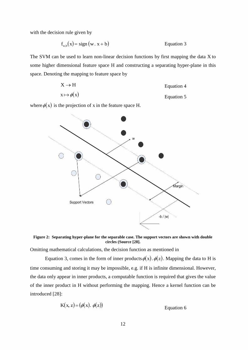
For training data that is linearly separable, a hyper-plane is constructed that separates the
positive from the negative examples with maximum margin. The points x which lie on the
hyper-plane satisfy 0. bxw , where w is normal to the hyper-plane, wb is the
perpendicular distance from the hyper-plane to the origin, and w is the Euclidean norm of
w (as shown in Figure 2). Let d (and d ) be the shortest distance from the separating
hyper-plane to the closest positive (negative) example, and define the “margin” of a
separating hyper-plane to be dd . For the linearly separable case, the support vector
algorithm simply looks for the separating hyper-plane with largest margin.
This can be formulated as follows: suppose that all the training data satisfy the following
constraints:
1,1. ii ybxw Equation 1
1,1. ii ybxw Equation 2
12
with the decision rule given by
bxwsignxf bw ., Equation 3
The SVM can be used to learn non-linear decision functions by first mapping the data X to
some higher dimensional feature space H and constructing a separating hyper-plane in this
space. Denoting the mapping to feature space by
HX Equation 4
xx Equation 5
where x is the projection of x in the feature space H.
Figure 2: Separating hyper-plane for the separable case. The support vectors are shown with double circles (Source [28].
Omitting mathematical calculations, the decision function as mentioned in
Equation 3, comes in the form of inner products zx . . Mapping the data to H is
time consuming and storing it may be impossible, e.g. if H is infinite dimensional. However,
the data only appear in inner products, a computable function is required that gives the value
of the inner product in H without performing the mapping. Hence a kernel function can be
introduced [28]:
zxzxK ., Equation 6

13
The kernel function allows constructing an optimal separating hyper-plane in the space H
without explicitly performing calculations in this space. Commonly used kernels include
[29]:
Polynomial kernel dyxyxK ,1,
Radial Basis Function (RBF) 222/exp, yxyxK
where is width of the kernel
Sigmoidal yxyxK .tanh, , with gain and offset
This is called „kernel trick‟ or „kernel approach‟ and gives the SVM great flexibility. With a
suitable choice of parameters, SVM can separate any consistent data set. For noisy data,
slack variables can be introduced to allow training errors.
In the following subsection we explain the main algorithms that have been used in the
OSVM framework and then in Section 2.4.3 we discuss other main Non-OSVM algorithms
to handle OCC problem.
2.4.2. One-class Support Vector Machine (OSVM)
The one-class classification problem is often solved by estimating the target density [4], or
by fitting a model to the data support vector classifier [13]. Tax and Duin [19,20] seek to
solve the problem of OCC by distinguishing the positive class from all other possible
patterns in the pattern space. They constructed a hyper-sphere around the positive class data
that encompasses almost all points in the data set with the minimum radius. This method is
called the Support Vector Data Description (SVDD).
Assume a data set containing N data objects, Nixi ,,2,1, and the hyper-sphere is
described by centre a and radius R (See Figure 3). To fit the hyper-sphere to the data, an
error function L is minimized that contains the volume of the hyper-sphere and the distance
from the boundary of the outlier objects. The solution is constrained with the requirement
that (almost) all data is within the hyper-sphere. In operation, an SVDD classifier rejects a
given test point as outlier if it falls outside the hyper- sphere. To allow the possibility of
outliers in the training set, the distance from ix to the centre a should not be strictly smaller
than R, but larger distances should be penalized. Therefore, slack variables ξ is introduced
which measure the distance to the boundary, if an object is outside the description. An extra

14
parameter C has to be introduced for the trade-off between the volume of the hyper-sphere
and the number of target objects accepted. This results in the following error and
constraints:
i
iCRaRL 2,, Equation 7
iii Rax ,22 Equation 8
Figure 3 : The hyper-sphere containing the target data, with centre a and radius R. Three objects are on the boundary are the support vectors. One object xi is outlier and has i > 0 (Source: Tax [2]).
In order to train this model, there is a possibility of rejecting some fraction of the positively-
labelled training objects, when volume of the hyper-sphere decreases. Furthermore, the
hyper-sphere model of the SVDD can be made more flexible by introducing kernel
functions. Tax [2] considers Polynomial and a Gaussian kernel and found that the Gaussian
kernel works better for most data sets (Figure 4). Tax uses different values for the width of
the kernel, s. The larger the width of the kernel, the fewer support vectors are selected and
the description becomes more spherical. In Figure 4 it can be seen that except for the
limiting case where s becomes very large, the description is tighter than the original
spherically shaped description or the description with the Polynomial kernels. Increasing s
decreases the number of support vectors. Also, using the Gaussian kernel instead of the
Polynomial kernel results in tighter descriptions, but it requires more data to support more
flexible boundary. Their method becomes inefficient when the data set has high dimension.
This method also doesn‟t work well when large density variation exist among the objects of
data set, in such case it starts rejecting the low-density target points as outliers. Tax shows
the usefulness of the approach on machine fault diagnostic data and handwritten digit data.

15
Figure 4 : Data description trained on a banana-shaped data set. The kernel is a Gaussian kernel with different width sizes s. Support vectors are indicated by the solid circles; the dashed line is the
description boundary (Source: Tax [2]).
Tax and Duin [1] suggest a sophisticated method which uses artificially generated outliers,
uniformly distributed in the hyper-sphere, to optimize the OSVM parameters in order to
balance between over-fitting and under-fitting. The fraction of the accepted outliers by the
classifier is an estimate of the volume of the feature space covered by the classifier. To
compute the error without the use of outlier examples, they uniformly generate artificial
outliers in and around the target class. If a hyper-cube is used then in high dimensional
feature space it becomes infeasible. In that case, the outlier objects generated from a hyper-
cube will have very low probability to be accepted by the classifier. The volume in which
the artificial outliers are generated has to fit as tight as possible around the target class. To
make this procedure applicable in high dimensional feature spaces, they propose to generate
outliers uniformly in a hyper-sphere. This is done by transforming objects generated from a
Gaussian distribution. Their experiments suggest that the procedure to artificially generate
outliers in a hyper-sphere is feasible for up to 30 dimensions.
Schölkopf et al. [30,31] present an alternative approach to the above-mentioned work of
Tax and Duin on OCC, using a separating hyper-plane. In their method they construct a
hyper-plane instead of a hyper-sphere around the data, such that this hyper-plane is
maximally distant from the origin and can separate the regions that contain no data. They
propose to use a binary function that returns +1 in „small‟ region containing the data and -1
elsewhere. For a hyper-plane w which separates the data ix from the origin with maximal
margin , the following holds
iiiixw ,0,. Equation 9

16
And the function to evaluate a new test object z becomes
zwIwzf .,, Equation 10
Schölkopf et al. [31] then minimizes the structural error of the hyper-plane measured by w
and some errors, encoded by the slack variable i are allowed. To separate the dataset from
the origin, a quadratic program needs to be solved. This results in the following
minimization problem
i
iNw 1
2
1min
2
Equation 11
with the constraints given by equation iiiixw ,0,. .
A variable ν is introduced that takes values between 0 and 1 that controls the effect of
outliers i.e. the hardness or softness of the boundary around the data. This variable ν can be
compared with the parameter C presented in the Tax‟s SVDD. Schölkopf et al. [31] suggest
the use of different kernels, corresponding to a variety of non-linear estimators. In practical
implementations, this method and the SVDD method of Tax [2] operate comparably and
both perform best when the Gaussian kernel is used. As mentioned by Campbell and
Bennett [32], the origin plays a crucial role in this method, which is a drawback since the
origin effectively acts as a prior for where the class abnormal instances are assumed to lie
(termed as the problem of origin). The method has been tested on both synthetic and real-
world data. Schölkopf et al. [31] present the efficacy of their method on the US Postal
Services dataset of handwritten digits. The database contains 9298 digit images of size
16×16=256; the last 2007 constitute the test set. They trained the algorithm using a Gaussian
kernel of width s=0.25, on the test set and used it to identify outliers. In their experiments,
they augmented the input patterns with ten extra dimensions corresponding to the class
labels of the digits, to help to identify mislabelled data as outliers. Their experiments show
that the algorithm indeed extracts patterns which are very hard to assign to their respective
classes and a number of outliers were in fact identified.
Manevitz and Yousef [33] investigate the usage of one-class SVM for information retrieval.
Their paper proposes a different version of the one-class SVM as proposed by Schölkopf et
al. [21], which is based on identifying outlier data as representative of the second class. The
idea of this methodology is to work first in the feature space, and assume that not only the
origin is member of the outlier class, but also all the data points close enough to the origin

17
are considered as noise or outliers (see Figure 5). Geometrically speaking, the vectors lying
on standard sub-spaces of small dimension i.e. axes, faces, etc., are to be treated as outliers.
Hence, if a vector has few non-zero entries, then this indicates that the pattern shares very
few items with the chosen feature subset of the database. Therefore, this item will not serve
as a representative of the class and will be treated as an outlier. Outliers can be identified by
counting features with non-zero values and if they are less than a predefined threshold. The
threshold can either be set globally or determined individually for different categories.
Linear, sigmoid, polynomial and radial basis kernels were used in this work. They evaluate
their results on the Reuters Data set [34] using the 10 most frequent categories. Their
results were generally somewhat worse than the OSVM algorithm presented by Schölkopf et
al. [21]. However they observe when the number of categories was increased, their version
of SVM obtains better results.
Figure 5 : Outlier SVM Classifier. The origin and small subspaces are the original members of the second class. The diagram is conceptual only (Source: Manevitz and Yousef [33]).
Li et al. [35] present an improved version of the OCC presented by Schölkopf et al. [21] for
detecting anomaly in an intrusion detection system, with higher accuracy than other
standard machine learning algorithms. Zhao et al. [36] used this method for customer churn
prediction for the wireless industry data. They investigate the performance of different
kernel functions for this version of one-class SVM, and show that the Gaussian kernel
function can detect more churners than the Polynomial and Linear kernel.

18
An extension to the work of Tax and Duin [19,20] and Schölkopf [30] is proposed by
Campbell and Bennett [32]. They present a kernel OCC algorithm that uses linear
programming techniques instead of quadratic programming. They construct a surface in the
input space that envelopes the data, such that the data points within this surface are
considered targets and outside it are regarded as outlier. In the feature space, this problem
condenses to finding a hyper-plane which is pulled onto the data points and the margin
remains either positive or zero. To fit the hyper-plane as tight as possible, the mean value of
the output of the function is minimized. To accommodate outliers, a soft margin can be
introduced around the hyper-plane. Their algorithm avoids the problem of origin (as is
apparent in the OCC algorithm presented by Schölkopf et al.[31]) by attracting hyper-plane
towards the centre of data distribution rather than by repelling it away from a point outside
the data distribution. Different kernels can be used to create hyper-planes; however they
showed that RBF kernel can produce closed boundaries in input space while other kernels
may not. A drawback of their method is that it is highly dependent on the choice of kernel
width parameter, However, if the data size is large and contains some outliers then can
be estimated. They showed their results on artificial data set, Biomed Data [37] and
Condition Monitoring data for machine fault diagnosis.
Yu [38] proposes a one-class classification algorithm with SVMs using positive and
unlabeled data and without labelled negative data and discuss some of the limitations of
other OCC algorithms [1][[33]. On the performance of OSVMs under such scenario of
learning with unlabeled data with no negative examples, Yu comments that to induce
accurate class boundary around the positive data set, OSVM requires larger number of
training data. The support vectors in such a case come only from positive examples and
cannot create proper class boundary, which also leads to overfitting and underfitting of the
data. Figure 6 (a) and (b) show the boundaries of SVM trained from positives and negatives
and OSVM trained from only positives on a synthetic data set in a two-dimensional space.
In this low-dimensional space, the ostensibly “smooth” boundary of OSVM is the result of
incomplete SVs due to not using the negative SVs, and not as a result of the good
generalization. This becomes much worse in high-dimensional spaces where more SVs
around the boundary are needed to cover major directions. When the numbers of SVs in
OSVM were increased, it overfits the data rather than being more accurate as shown in
Figure 6 (c) and (d). However, such OSVM boundary might be the best achievable one
when only positive data are available. Yu [39] presents an OCC algorithm called Mapping

19
Convergence (MC) to induce accurate class boundary around the positive data set in the
presence of unlabeled data and without negative examples. The algorithm has two phases:
mapping and convergence. In the first phase, a weak classifier (e.g. Rocchio [40][41]) is
used to extract strong negatives from the unlabeled data. The strong negatives are those
examples that are far from the class boundary of the positive data. In the second phase, a
base classifier (e.g. SVM) is used iteratively to maximize the margin between positive and
strong negatives for better approximation of the class boundary. Yu [39] also presents
another algorithm called Support Vector Mapping Convergence (SVMC) that works faster
than the MC algorithm. At every iteration, SVMC only uses minimal data such that the
accuracy of class boundary is not degraded and the training time of SVM is also saved.
However, the final class boundary is slightly less accurate than the one obtained by
employing MC. They show that MC and SVMC perform better than other OCC algorithms
and can generate accurate boundaries comparable to standard SVM with fully labelled data.
Figure 6 : Boundaries of SVM and OSVM on a synthetic data set: big dots: positive data, small dots: negative data (Source Yu, H. [38])

20
2.4.3. One-Class Classifiers other than OSVMs
2.4.3.1. One-Class Classifier Ensembles
As in the normal classification problems, one classifier hardly ever captures all
characteristics of the data. However, using just the best classifier and discarding the
classifiers with poorer performance might waste valuable information [42]. To improve the
performance of different classifiers which may differ in complexity or training algorithm, an
ensemble of classifiers is a viable solution. This may not only increase the performance, but
can also increase the robustness of the classification [43]. Classifiers are commonly
ensembled to provide a combined decision by averaging the estimated posterior
probabilities. This simple algorithm already gives very good results for multi-class problems
[44]. When Bayes‟ theorem is used for the combination of different classifiers, under the
assumption of independence, a product combination rule can be used to create a classifier
ensemble. The outputs of the individual classifiers are multiplied and then normalized (this
is also called the logarithmic opinion pool [45]). In the combination of one-class classifiers,
the situation is different. One-class classifiers cannot directly provide posterior probabilities
for target (positive class) objects, because accurate information on the distribution of the
outlier data is not available. In most cases, however, assuming that the outliers are
uniformly distributed, the posterior probability can be estimated. Tax [2] mentions that in
some OCC methods distance is estimated instead of probability. If there exists a
combination of distance and probability outputs, the outputs should be standardized before
they can be combined. To use the same type of combining rules as in conventional
classification ensembles, the distance measures must be transformed into a probability
measure. As a result, combining in OCC improves performance, especially when the
product rule is used to combine the probability estimates. Classifiers can be combined in
many ways. One of the ways is to use different feature sets and to combine classifiers
trained on each of them. Another way is to train several classifiers on one feature set. Since
the different feature sets contain much independent information, combining classifiers
trained in different feature spaces provide better accuracy.
Tax and Duin [46] investigate the influence of the feature sets, their inter-dependence and
the type of one-class classifiers for the best choice of the combination rule. They use a
normal density and a mixture of Gaussian and the Parzen density estimation [9] as two types
of one-class classifiers. They use four models, the SVDD [20], K-means clustering [9], K-

21
center method [47] and an auto-encoder neural network [10]. The Parzen density estimator
emerged as the best individual one-class classifier on the handwritten digit pixel dataset
[48]. They showed that combining classifiers trained in different feature spaces is useful. In
their experiments, the product combination rule gave the best results. The mean combination
rule suffers from the fact that the area covered by the target set tends to be overestimated.
As a result of that more outlier objects may be accepted than it is necessary.
Juszczak and Duin [49] extend combining one-class classifier for classifying missing data.
Their idea is to form an ensemble of one-class classifiers trained on each feature, pre-
selected group of features or to compute a dissimilarity representation from features. The
ensemble should be able to predict missing feature values based on the remaining classifiers.
As compared to standard methods, their method is more flexible, since it requires much
fewer classifiers and do not require re-training of the system whenever missing feature
values occur. They also show that their method is robust to small sample size problems due
to splitting the classification problem to several smaller ones. They compare the
performance of their proposed ensemble method with standard methods used with missing
features values problem on several UCI datasets [50]. Lai et al. [51] study combining one-
class classifier for image database retrieval and showed that combining SVDD-based
classifiers improves the retrieval precision. Ban and Abe [52] address the problem of
building multi class classifier based on one-class classifiers ensemble. They studied two
kinds of once class classifiers, namely, SVDD [20] and Kernel Principal Component
Analysis [53]. They constructed a minimum distance based classifiers from an ensemble of
one-class classifiers that is trained from each class and assigns a test sample to a given class
based on its prototype distance. Their method gave comparable performance as SVMs on
some benchmark data sets; however it is heavily dependent on the algorithm parameters.
They also commented that their process could lead to faster training and better
generalization performance provided appropriate parameters are chosen.
Boosting methods have been successfully applied to classification problems [54]. Their high
accuracy, ease of implementation and wide applicability make them as a suitable choice
among machine learning practitioners. Rätsch et al. [55] propose a boosting-like one-class
classification algorithm based on a technique called barrier optimization [56]. They also
show an equivalence of mathematical programs that a support vector algorithm can be
translated into an equivalent boosting-like algorithm and vice versa. It has been pointed out
by Schapire et al. [57] that boosting and SVMs are „essentially the same‟ except for the way

22
they measure the margin or the way they optimize their weight vector: SVMs use the l2-
norm and boosting employs the l1-norm. SVMs use the l2-norm to implicitly compute scalar
products in feature space with the help of kernel trick, where as boosting perform
computation explicitly in feature space. They comment that SVMs can be thought of as a
„boosting‟ approach in high dimensional feature space spanned by the base hypotheses.
Rätsch et al. [55] exemplify this translation procedure for a new algorithm called the one-
class leveraging. Building on barrier methods, a function is returned which is a convex
combination of the base hypotheses that leads to the detection of outliers. They commented
that that the prior knowledge that is used by boosting algorithms for the choice of weak
learners can be used in one-class classification. They show the usefulness of their results on
artificially generated toy data and the US Postal Service database of handwritten characters.
2.4.3.2. Neural Networks
Ridder et al. [58] conduct an experimental comparison of various OCC algorithms. They
compare a number of unsupervised methods from classical pattern recognition to several
variations on a standard shared weight supervised neural network [59] proposed by Viennet
[60]. The following unsupervised methods were included in their study:
a) Global Gaussian approximation
b) Parzen density estimation
c) 1-Nearest Neighbour method
d) Local Gaussian approximation (combines aspects of a) and c)).
They use samples from scanned newspaper images (at 600 dpi) as experimental datasets.
The binary images were then reduced six-fold to approximately 1000×750 pixel grey value
images. They show that Gaussian methods give the worst results, while the Parzen method
suffers less from the problems of the Gaussian method. The 1- Nearest Neighbor method
very clearly distinguishes the images from text better than any other method. The Local
Gaussian performs much worse than the Parzen and the 1-nearest neighbor method, but it
outperforms the simple Gaussian method. It is also the only method which does not suffer
from the fact that background is classified as text. They also show that adding a layer with
radial basis function improves performance.
Manevitz and Yousef [61] show how a simple neural network can be trained to filter
documents when only positive information is available. In their design of the filter, they
used a basic feed-forward neural network. To incorporate the restriction of availability of

23
only positive examples, they used the design of a feed forward network with a “bottleneck”.
They chose three level network with m input neurons, m output neurons and k hidden
neurons, where k < m. The network is trained using standard back-propagation algorithm
[62] to learn the identity function on the positive examples. The idea is that while the
bottleneck prevents learning the full identity function on m-space; the identity on the small
set of examples is in fact learnable. The set of vectors for which the network acts as the
identity function is a sort of sub-space which is similar to the trained set. For testing a given
vector, it is shown to the network, if the result is the identity; the vector is deemed
interesting i.e. positive or else an outlier. Manevitz and Yousef [63] apply the auto-
associator neural network to document classification problem. To determine acceptance
threshold, they used a method based on a combination of variance and calculating the
optimal performance. During training, they check the performance values of the test set at
different levels of error. The training process is stopped at the point where the performance
starts a steep decline. Then they perform a secondary analysis to determine an optimal real
multiple of the standard deviation of the average error that serves as a threshold. The
method was tested and compared with a number of competing approaches, i.e. Neural
Network, Naïve Bayes, Nearest Neighbour, Prototype algorithm, and shown to outperform
them.
Skabar [64] describes to learn a classifier based on feed-forward neural network using
positive examples and corpus of unlabeled data containing both positive and negative
examples. In conventional feed forward binary neural network classifier, positive examples
are labelled as 1 and negative examples as 0. The output of the network represents the
probability that an unknown example belongs to the target class, with threshold of 0.5 is set
to decide whether an unknown sample belongs to either of the case. However, in this case,
since unlabeled data contain some unlabeled positive examples, the output of the trained
neural network may be less than or equal to the actual probability that an example belongs
to the positive class. If it is assumed that the labelled positive examples adequately represent
the positive concept, it can be hypothesized that the neural network will be able to draw a
class boundary between negative and positive examples. Skabar shows [64] the application
of the technique to the prediction of mineral deposit location.
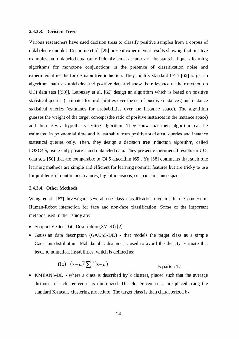
24
2.4.3.3. Decision Trees
Various researchers have used decision tress to classify positive samples from a corpus of
unlabeled examples. Decomite et al. [25] present experimental results showing that positive
examples and unlabeled data can efficiently boost accuracy of the statistical query learning
algorithms for monotone conjunctions in the presence of classification noise and
experimental results for decision tree induction. They modify standard C4.5 [65] to get an
algorithm that uses unlabeled and positive data and show the relevance of their method on
UCI data sets [[50]]. Letouzey et al. [66] design an algorithm which is based on positive
statistical queries (estimates for probabilities over the set of positive instances) and instance
statistical queries (estimates for probabilities over the instance space). The algorithm
guesses the weight of the target concept (the ratio of positive instances in the instance space)
and then uses a hypothesis testing algorithm. They show that their algorithm can be
estimated in polynomial time and is learnable from positive statistical queries and instance
statistical queries only. Then, they design a decision tree induction algorithm, called
POSC4.5, using only positive and unlabeled data. They present experimental results on UCI
data sets [50] that are comparable to C4.5 algorithm [65]. Yu [38] comments that such rule
learning methods are simple and efficient for learning nominal features but are tricky to use
for problems of continuous features, high dimensions, or sparse instance spaces.
2.4.3.4. Other Methods
Wang et al. [67] investigate several one-class classification methods in the context of
Human-Robot interaction for face and non-face classification. Some of the important
methods used in their study are:
Support Vector Data Description (SVDD) [2]
Gaussian data description (GAUSS-DD) - that models the target class as a simple
Gaussian distribution. Mahalanobis distance is used to avoid the density estimate that
leads to numerical instabilities, which is defined as:
1 xxxf T
Equation 12
KMEANS-DD - where a class is described by k clusters, placed such that the average
distance to a cluster centre is minimized. The cluster centres ci are placed using the
standard K-means clustering procedure. The target class is then characterized by

25
2min ii
cxxf Equation 13
The above two classifiers are defined as:
otherwiseiftargetnon
thresholdxtMeasuremeniftargetxClass
,
;,
The PCA-DD method, based on Principal Component Analysis, describes the target data
by a linear subspace defined by the eigenvectors of the data covariance matrix Σ. Only k
eigenvectors are used, which are stored in a d×k matrix W (where d is the dimensionality
of the original feature space). To check if a test object is outlier, the reconstruction error
is computed, which is the difference between the original object and its projection onto
the subspace. This projection is computed by:
XT
proj WWWW1
Equation 14
The reconstruction error is then given by 2
projxxf
LP-DD is a linear programming method [68]. This data descriptor is constructed to
describe target classes that can be represented in terms of distances to a set of support
objects. This classifier uses the Euclidean distance by default. This classifier has the
following form ii xxdwxf , . The weights wi are optimized such that just a few
weights stay non-zero, and the boundary is as tight as possible around the data,
Wang et al. [67] study the performance of these one-class classification methods on the
object recognition dataset described in Wang and Lopes [69]. This dataset contains two
parts. There are 400 pictures from AT&T/ORL face database [70] and 402 non-face pictures
from their previous work [71]. They resize all patterns to 32×32 and all the experiments
were carried out based on the PRTOOLS [72] and DDTOOLS [2]. For their analysis, they
set face as the target class. In their experimentation they observe that SVDD attains better
performance in comparison to other studied OCC methods. They comment that the good
performance of SVDD in comparison to other methods can be attributed to its flexibility.
The other methods use very strict models, such as planar shapes. They also investigate the
effect of varying the number of features. They remark that more features do not always
guarantee better results, because with an increase in the number of features, more training
data are needed to reliably estimate the class models.
Ercil and Buke [73] report a different technique to tackle the OCC problem, based on fitting
an implicit polynomial surface to the point cloud of features, to model the target class to
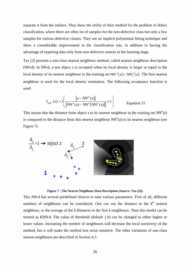
26
separate it from the outliers. They show the utility of their method for the problem of defect
classification, where there are often lot of samples for the non-defective class but only a few
samples for various defective classes. They use an implicit polynomial fitting technique and
show a considerable improvement in the classification rate, in addition to having the
advantage of requiring data only from non-defective motors in the learning stage.
Tax [2] presents a one-class nearest neighbour method, called nearest neighbour description
(NN-d). In NN-d, a test object z is accepted when its local density is larger or equal to the
local density of its nearest neighbour in the training set zNNzNN trtr1 . The first nearest
neighbour is used for the local density estimation. The following acceptance function is
used:
1)()(
)()(
zNNNNzNN
zNNzIzf
trtrtr
tr
NNtr Equation 15
This means that the distance from object z to its nearest neighbour in the training set NNtr(z)
is compared to the distance from this nearest neighbour NNtr(z) to its nearest neighbour (see
Figure 7).
Figure 7 : The Nearest Neighbour Data Description (Source: Tax [2]).
This NN-d has several predefined choices to tune various parameters. First of all, different
numbers of neighbours can be considered. One can use the distance to the kth nearest
neighbour, or the average of the k distances to the first k neighbours. Then this model can be
termed as KNN-d. The value of threshold (default 1.0) can be changed to either higher or
lower values. Increasing the number of neighbours will decrease the local sensitivity of the
method, but it will make the method less noise sensitive. The other variations of one-class
nearest neighbours are described in Section 4.3.

27
Tax and Duin [74] proposes a nearest neighbour method capable of finding data boundaries
when the sample size is very low. The boundary thus constructed can be used to detect the
targets and outliers. The method compares the distance from a test object to the training set
to the nearest neighbour distance within the training set. This method has the disadvantage
that it relies on the individual positions of the objects in the target set. Their method seems
to be useful in situations where the data is distributed in subspaces. They tested the
technique on both real and artificial data and found to be very useful when very little
amount of training data exist (less than 5samples per feature).
Datta [75] modify the standard nearest neighbour algorithm [76] appropriate to learn a
single class, called the positive class. The modified algorithm, NN-PC (nearest neighbour
positive class), takes examples from only one-class as input. NN-PC learns a constant
which is the maximum distance a test example can be from any learned example and still be
considered a member of the positive class. Any test example that has a distance greater than
from any training example will not be considered a member of the positive class. is
calculated by
yxdistxyMinxMax , Equation 16
where x and y are two examples of the positive class, and Euclidean distance (dist(…)) is
used as the distance function.
While classifying test examples, if it varies too much from the positive examples, then it is
classified as an outlier. Mathematically, if testxdistx ,: then the test example is
classified as member of the positive class, otherwise it is not. Datta also experimented with
another similar modification called NN-PCN, that involves learning a vector n ,1
,where i is the threshold for the ith example. This modification records the distance to the
closest example for each example. i is calculated by
yxdistxyMin iii , Equation 17
where ix is the ith training example. To classify a test example same classification rule as
above is used, that is, if iii testxdistx ,: then the test example is classified as a
member of the positive class.
Datta [75] also suggests a method to learn a Naive Bayes classifier from samples of positive
class data only. Traditional Naive Bayes [76] attempts to find nni vAvACp &&| 11 ,

28
that is, the probability of a class given an unlabeled example. By assuming that the attributes
are independent and applying Bayes' theorem the previous calculation is proportional to:
ia ttr ibutes
jij CpCvAp
| Equation 18
where Aj is an attribute, v is a value of the attribute, Ci is a class, and the probabilities are
estimated using the training examples.
When only the positive class is available, the calculation of iCp (from Equation 18)
cannot be done correctly. Datta [75] modify Naive Bayes to learn in a single class situation
and call their modification as NB-PC (Naive Bayes Positive Class) that uses the
probabilities of the attribute-values. NB-PC computes a threshold t as
attr ibutes
jij vApxMint Equation 19
where ij vA is the attribute value for the example x and ij vAp is the probability of the
attribute's ith value. The probabilities for the different values of attribute Aj is normalized by
the probability of the most frequently occurring v. During classification, if for the test
example tvAattributes
jij , then the test example is predicted as a member of the positive
class. Datta tested the above positive class algorithms on various data sets taken from UCI
repository [50] and conclude that NN-PCN seems to perform the worst, since it typically has
precision and recall values lower than other discussed algorithms. Learning a different for
each example does not intuitively seem like a reliable or stable way of predicting class
membership, since s can easily change depending on the training examples. They also
observed that NN-PC and NB-PC have classification accuracy (both precision and recall
values) close to C4.5‟s [65] value, although C4.5 was learning from all classes and they
were learned using only one-class.
2.5. Category 3: Application Domain Applied
2.5.1. Text / Document Classification
Traditional text classification techniques require an appropriate distribution of positive and
negative examples to build a classifier; thus they are not suitable for this problem of OCC. It
is of course possible to manually label some negative examples, though depending on the

29
application domain, this may be a labour-intensive and a time consuming task. However, the
core problem remains, that it is difficult or impossible to compile a set of negative samples
that provides a comprehensive characterization of everything that is `not' the target concept,
as is assumed by a conventional binary classifier. It is a common practice to build text
classifiers using positive and unlabeled examples3 as collecting unlabeled samples is
relatively easy and fast in many text or Web page domains [27], [78]. In this subsection, we
will discuss some of the algorithms that exploit this methodology with application to text
classification.
The ability to build classifiers without negative training data is useful in a scenario if one
needs to extract positive documents from many text collections or sources. Liu et al. [27]
propose a method (called Spy EM) to solve this problem in the text domain. It is based on
Naïve Bayesian classification (NB) and the Expectation Maximization (EM) algorithm [79].
The main idea of the method is to first use a technique to identify some reliable / strong
negative documents from the unlabeled set. It then runs EM to build the final classifier. Yu
et al. [3,80] propose a SVM based technique called PEBL (Positive Example Based
Learning) to classify Web pages with positive and unlabeled pages. Once a set of strong
negative documents is identified, SVM is applied iteratively to build a classifier. PEBL is
sensitive to the number of positive examples. When the positive data is small, the results are
often very poor. Li and Liu [17] propose an alternative method to learn to classify texts
using positive and unlabeled data. Their method differs from PEBL in that they perform
negative data extraction from the unlabeled set using the Rocchio method [40]4. Although
the second step also runs SVM iteratively to build a classifier, there is a key difference in
selection of final classifier. Their technique selects a „good‟ classifier from a set of
classifiers built by SVM, while PEBL does not. Liu et al. [16] study the same problem and
suggest that many algorithms that build text classifier with positive and unlabeled data are
based on two strategies:
3 For further reading on this topic , readers are advised to refer to survey paper by Zhang and Zuo [77] 4 The basic idea of the algorithm is to represent each document, e, as a vector in a vector space so that
documents with similar content have similar vectors. The value ei of the ith key-word is represented as the tf-idf
weight [81]
30
Identifying a set of reliable / strong negative documents from the unlabeled set. In this
step, Spy-EM [27] uses a Spy technique, PEBL uses a technique called 1-DNF [3], and
Roc-SVM [16] uses the Rocchio algorithm [40].
Building a set of classifiers by iteratively applying a classification algorithm and then
selecting a good classifier from the set. In this step, Spy-EM uses the Expectation
Maximization (EM) algorithm with a NB classifier, while PEBL and Roc-SVM use
SVM. Both Spy-EM and Roc-SVM have some methods for selecting the final classifier.
PEBL simply uses the last classifier at convergence, which can be a poor choice.
These two steps together work in an iterative manner to increase the number of unlabeled
examples that are classified as negative, while at the same time maintain the correct
classification positive examples. It was shown theoretically by Liu et al. [27] that if the
sample size is large enough, maximizing the number of unlabeled examples classified as
negative while constraining the positive examples to be correctly classified will give a good
classifier. Liu et al. [16] introduce two new methods, one for Step 1 (i.e. the Naïve Bayes
method) and Step 2 (i.e. SVM alone) and perform an evaluation of all 16 possible
combinations of methods for Step 1 and Step 2 (discussed above). They develop a
benchmarking system called LPU (Learning from Positive and Unlabeled data) [82]. They
also propose an approach based on a biased formulation of SVM that allows noise (or error)
in positive examples. This soft margin version of biased-SVM uses two parameters, C and
C respectively, to weight both positive and negative errors differently. It can be expressed
mathematically as:
1
1
1
12
1 k
ii
k
ii
T CCwwMaximizing
Equation 20
Subject to: nibxwy iiT
i ,2,1,1
nii ,2,1,0
They experiment on two data sets, namely Reuters [34] and Usenet articles as compiled by
Lang [83], and conclude that the biased-SVM approach outperforms all existing two-step
techniques.
Yu et al. [84] explore SVMC [38,39] (for detail on this technique refers to Section 2.4.2) for
performing text classification without labelled negative data. They use two commonly used
corpora for text classification – Reuters [34] and WebKb [85] and compare their method

31
against six other methods: (1) Simple Mapping Convergence (MC); (2) OSVM; (3)
Standard SVM trained with positive examples and unlabeled documents substituted for
negative documents; (4) Spy-EM; (5) Naïve Bayes with Negative noise; (6) Ideal SVM
trained from completely labelled documents. In their results they show that with a
reasonable amount of positive documents, the MC algorithm gives the best results among all
the methods considered. Their analysis shows that when the positive training data is not
under-sampled, SVMC significantly outperforms other methods because SVMC tries to
exploit the natural gap between positive and negative documents in the feature space, which
eventually helps to improve the generalization performance.
Peng et al. [86] present a text classifier from positive and unlabeled documents based on
Genetic Algorithms (GA) by adopting a two stage strategy (as discussed above). Firstly,
reliable negative documents were identified by improved 1-DNF algorithm. Secondly, a set
of classifiers were built by iteratively applying SVM algorithm on training example sets.
Thirdly, they discuss an approach to evaluate the weighted vote of all classifiers generated
in the iteration steps to construct the final classifier based on a GA. They comment that the
GA evolving process can discover the best combination of the weights. Their problem
statement is shown in Figure 8. They perform experiments on the Reuter data set [34] and
compare their results against PEBL [80] and OSVM and showed that their GA based
classification performs better.

32
Figure 8 : Illustration of the procedure to build text classifiers from labeled and unlabeled examples based on GA. Ci represents the individual classifier produced by the ith iteration of the SVM algorithm.
(Source: Peng et al. [86]).
Pan et al. [87] extend the concept of classifying positive examples with unlabeled samples
in the Collaborative Filtering (CF) application. In CF, the positive data is gathered based on
user interaction with the web like news items recommendation or bookmarking pages etc.
However, due to ambiguous interpretations, limited knowledge or lack of interest of users,
the collection of valid negative data gets hampered. Sometime negative and unlabeled
positive data are severely mixed up and difficult to discern. Manually labelling negative
data is not only intractable considering the size of the web but also will be poorly sampled.
Traditional CF algorithms either label negatives data, or assume missing data as negative.
Both of these approaches have their inherent problem of being expensive and biasing the
recommendation results. Pan et al. [87] propose two approaches to one-class CF to handle
the negative sparse data to balance the extent to which to treat missing values as negative
examples. The first approach is based on weighted low rank approximation [88] that works
on the idea of providing different weights to error terms of both positive and negative
examples in the objective function. The second is based on sampling some missing values as
negative examples based on some sampling strategies. They perform their experimentation

33
on real life data from social bookmarking site del.icio.us and Yahoo News data set and show
that their method outperforms other state of the art CF algorithms.
Onoda et al. [89] report a document retrieval method using non-relevant documents. Users
rarely provide a precise query vector to retrieve desired documents in the first iteration. In
subsequent iterations, the user evaluates whether the retrieved documents are relevant or
not, and correspondingly the query vector is modified in order to reduce the difference
between the query vector and documents evaluated as relevant by the user. This method is
called relevance feedback. The relevance feedback needs a set of relevant and non-relevant
documents to work usefully. However, sometimes the initial retrieved documents that are
presented to a user do not include relevant documents. In such a scenario, traditional
approaches for relevance feedback document retrieval systems do not work well, because
the systems need relevant and non relevant documents to construct a binary classification
problem. To solve this problem, Onoda et al. propose a feedback method using information
of non-relevant documents only, called non-relevance feedback document retrieval. A
diagrammatic representation of the problem of non relevance feedback is shown in Figure 9.
Their design of non-relevance feedback document retrieval is based on OSVM [21]. Their
proposed method selects documents which are discriminated as not non-relevant and near
the discriminant hyper-plane between non-relevant document and not non-relevant
documents. In their experiments they compare their approach with conventional relevance
feedback methods and vector space model without feedback. Their method gives
consistently better performance than other compared methods. They comment that this
method is very useful to retrieve relevant documents using information of non-relevant
documents only.
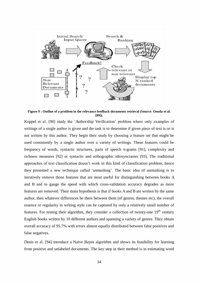
34
Figure 9 : Outline of a problem in the relevance feedback documents retrieval (Source: Onoda et al. [89]).
Koppel et al. [90] study the „Authorship Verification‟ problem where only examples of
writings of a single author is given and the task is to determine if given piece of text is or is
not written by this author. They begin their study by choosing a feature set that might be
used consistently by a single author over a variety of writings. These features could be
frequency of words, syntactic structures, parts of speech n-grams [91], complexity and
richness measures [92] or syntactic and orthographic idiosyncrasies [93]. The traditional
approaches of text classification doesn‟t work in this kind of classification problem, hence
they presented a new technique called „unmasking‟. The basic idea of unmasking is to
iteratively remove those features that are most useful for distinguishing between books A
and B and to gauge the speed with which cross-validation accuracy degrades as more
features are removed. Their main hypothesis is that if books A and B are written by the same
author, then whatever differences be there between them (of genres, themes etc), the overall
essence or regularity in writing style can be captured by only a relatively small number of
features. For testing their algorithm, they consider a collection of twenty-one 19th century
English books written by 10 different authors and spanning a variety of genres. They obtain
overall accuracy of 95.7% with errors almost equally distributed between false positives and
false negatives.
Denis et al. [94] introduce a Naïve Bayes algorithm and shows its feasibility for learning
from positive and unlabeled documents. The key step in their method is in estimating word

35
probabilities for the negative class because negative examples were not available. This
limitation can be overcome by assuming an estimate of the positive class probability (the
ratio of positive documents in the set of all documents). In practical situations, the positive
class probability can be empirically estimated or provided by domain knowledge. Their
results on WebKB data set [85] show that error rates of Naïve Bayes classifiers obtained
from p positive examples, PNB (Positive Naïve Bayes), trained with enough unlabeled
examples are lower than error rates of Naïve Bayes classifiers obtained from p labeled
documents. Denis et al. [95] consider situations where only a small set of positive data is
available together with unlabeled data. Constructing an accurate classifier in these situations
may fail because of the shortage of properly sampled data. However, learning in this
scenario may still be possible using the co-training framework (introduced by Blum and
Mitchell [22], and described earlier in Section 2.3), that looks for two views over the data.
For example, in the case of retrieval of bibliographic references, the positive examples are
stored in the user database. A first view of the bibliographic fields consists of - title, author,
abstract, editor. A second view is the full content of the paper. Unlabeled examples are
easily available in the bibliographic databases accessible via the World Wide Web. Co-
training algorithms incrementally build basic classifiers over each of the two feature sets.
They define a Positive Naïve Co-Training algorithm, PNCT that takes a small pool of
positive documents as it seed. PNCT first incrementally builds Naive Bayes classifiers from
positive and unlabeled documents over each of the two views by using PNB. Along the co-
training steps, self-labelled positive examples and self-labelled negative examples are added
to the training sets. They also propose a base algorithm which is a variant of PNB, able to
use these self-labelled examples. They perform experiments on the WebKB dataset [85] and
show that co-training algorithms lead to significant improvement of classifiers, even when
the initial seed is only composed of positive documents.
2.5.2. Other Application Domain
In this subsection we will highlight some of the other applications domains where
methodologies based on one-class classification have been utilized.
OSVMs have been successfully applied in a wide variety of application domains such as
Handwritten Digit Recognition [1,2,30], Information Retrieval [33], Classifying Missing
Data [49], Image Database Retrieval [1,96-98], Face Recognition Applications [67,99,100],
Chemometrics [101], Spectroscopy [102][103] Classification of Bio-Acoustic Time Series

36
[104], Nosocomial Infection Detection [105], Medical Analysis [106-108], Bioinformatics
[109-113], Steganalysis [114], Spam Detection [115,116], Detecting Anomalous Windows
Registry Access [117], Audio Surveillance [118], Ship Detection [119], Collision Detection
[120], Anomaly Detection [35,121-126], Yeast Regulation Prediction [127], Customer
Churn Detection [36], Relevant Sentence Extraction [128], Machine Vibration Analysis
[129], Machine Fault Detection [73,129-132] and Recommendation Tasks [133].
Compression neural networks for one-sided classification have been used in many areas,
these include detecting Mineral Deposits [64], fMRI Analysis [134] etc. One-class Fuzzy
ART networks have been explored by Murshed et al. [135] to classify Cancerous Cells.
Wang and Stolfo have used one-class Naïve Bayes to detect Masquerade Detection [136] in
a network and showed that less effort in data collection is required with comparable
performance as that of a multi-class classifier. Munroe and Madden [137] have presented a
one-class k-nearest neighbour approach for vehicle recognition from images and showed
that the results are comparable to that of standard multi-class classifiers.
2.6. Open Research Questions in OCC
The goal of One-Class Classification is to induce classifiers when only one class (the
positive class) is well characterized by the training data. In this chapter, we have presented a
survey of current state-of-the-art research work using OCC. We observe that the research
carried out in OCC can be broadly presented by three different categories or areas of study,
which depends upon the availability of training data, classification algorithms used and the
application domain investigated. Under each of these categories, we further provide details
of commonly used OCC algorithms. Although the OCC field is becoming mature, still there
are several fundamental problems that are open for research, not only in describing and
training classifiers, but also in scaling, controlling errors, handling outliers, using non-
representative sets of negative examples, combining classifiers and reducing dimensionality.
Classifier ensembles have not been exploited very much for OCC problems, and techniques
such as boosting and bagging deserve further attention. Another point to note here is that in
OSVMs, the kernels that have been used mostly are Linear, Polynomial, Gaussian or
Sigmoidal. We suggest it would be fruitful to investigate some more innovative forms of
kernels, for example Genetic Kernels [138] or domain specific kernels (for spectroscopic
data), for example, Weighted Linear Spectral Kernel [139], that have shown greater
potential in standard SVM classification. The kernels have been used as distance metric in

37
multi-class classification problems; however, the same is not exploited for the OCC. This
particular problem is investigated in the Chapter 4 of this thesis. In the case where abundant
unlabeled examples and some positive examples are available, researchers have used many
two-step algorithms (as have been discussed in Section 2.5.1). We believe that a Bayesian
Network approach to such OCC problems would be an interesting exercise.
This survey provides a broad insight into the study of the field of OCC. Depending upon the
data availability, algorithm use and application, appropriate OCC techniques can be applied
and improved upon. We hope that this survey will provide researchers with a direction to
formulate future novel work in this field and reduce their research time and effort
considerably.

38
Chapter 3
Spectral Data, Similarity Metrics and
Library Search
This chapter presents a brief description of the Raman Spectroscopy and the spectral data
thus obtained, followed by short review of the common spectral search and comparison
algorithms. This chapter highlights some standard spectral search and comparison methods,
and some recent / non-standard methods for finding similarity between spectra. A few
similarity measures that are specific for comparing the spectra are also introduced in this
chapter. The spectrum-specific comparison methods will be used to develop kernels to be
used in Chapter 4.
In our present research work we are interested in vibrational spectroscopy and related
techniques; therefore we have restricted our review, study and analysis of similarity and
search methods that have been applied in those fields, especially the sub-field of Raman
Spectroscopy.
3.1. Raman Spectroscopy
Raman Spectroscopy is a spectroscopy technique which is based on scattering of
monochromatic light in the visible, near infrared, or near ultraviolet range [12]. When a
chemical substance is illuminated by a laser, most of the light is elastically scattered due
Rayleigh scattering. A small portion of the light (1 in 106), however, is inelastically scattered
at a different wavelength to the incident light. This inelastic scattering of incident light is
known as Raman scattering. This scattering is due to the interaction of light with the
vibrational and rotational motions of molecules and other low-frequency modes within the
material. A Raman spectrum is thus obtained which shows the change in frequency of the
scattering light as well as its intensity. This Raman scattering can be treated as a „molecular
fingerprint‟ of a given chemical substance providing information on the vibrational and
rotational motions of the chemical bonds between the molecules (see Figure 10). Every

39
substance has a unique Raman spectrum and for machine learning tasks, this „molecular
fingerprint‟ can be exploited for unambiguous identification of substances.
Figure 10: Raman Spectrum of Azobenzene polymer (Source Horiba Scientific [140]
Each point in a Raman spectrum (see Figure 10) represents the value of intensity
corresponding to particular frequency. The Raman shift is either represented as wavelengths
or wavenumbers. The wavenumber is defined as number of waves per unit length [141],
which is directly proportional to the frequency of the scattered light (wavelength is inversely
proportional to the frequency). The wavenumber unit, cm-1, is commonly used.
Raman Spectroscopy has been used in wide variety of applications, such as gemstone
identification [142], identification and quantification of narcotics [143] and illicit substances
[144], chemical identification [145], and explosive detection [146].
Raman spectra can also be used to determine the quantity of a particular chemical substance
or estimate its presence within a mixture of various substances [139]. Figure 11 shows
Raman spectra of three different compounds, namely, Caffeine, Glucose and Cocaine. It can
be seen that all the three pure compounds have distinctive Raman spectra.

40
3.2. Some Definitions
In this section, we provide some basic definitions of the terms and concepts we will be using
in this and subsequent chapters.
Figure 11: Raman Spectra of three different compounds (Source: [139])
3.2.1. Similarity
Similarity can be defined as a degree of symmetry (quantitative or qualitative) between two
or more objects. In text recognition, it can be defined as number of matching characters
between two text strings. In Bioinformatics, it can be defined as the number of matching
DNA sequences. In geometrical application, it can be expressed as a score that represents
some kind of resemblance between two vectors. For spectroscopic data, similarity means
matching of peaks and overall shape of the spectrum. Common similarity measures are
Cosine and Correlation Coefficient. Each of these measures computes similarity between
spectra in its own way (for details refer to Section 3.4).

41
3.2.2. Dissimilarity
Dissimilarity can be defined as a degree of being distinct or unlike. In geometry, it can be
represented as a distance score (Manhattan, Euclidean, Mahalanobis, Chebychev etc)
between two or more vectors. The more dissimilar two vectors are the higher the value of
score. If two vectors are less dissimilar or bear more resemblance to each other than the
dissimilarity score will be low or close to zero.
Note: Similarity and Dissimilarity can be treated as reciprocal concepts in terms of
interpreting the value of score.
3.2.3. Comparison
Comparison means comparing two spectra based on some similarity or dissimilarity measure
and computes a score. This score can be used to access the degree of resemblance between
two spectra and can be employed in a library search (defined below).
3.2.4. Search
In spectroscopy, usually an unknown spectrum is searched against a known library of pure
substance to find a match (or nearest matches), called hits, for further analysis [147]. The
unknown spectrum is searched for using a search algorithm (see Section 3.4 to 3.6) which
computes a score based on similarity or dissimilarity measure it employs and provides a score
and a list of nearest matches.
3.2.5. Spectral Library
A spectral library is a database of spectra of known substances [147]. The spectral library is
usually used for spectrum search and comparison purposes and as an aid to identify unknown
spectrum. The companies that sell digitized spectral libraries for use by researchers and other
practitioners include Thermo Scientific, Sigma Aldrich, Bio-Rad Laboratories - Sadtler
Division, National Institute of Standards and Technology and many others. Spectral libraries
can also be developed within organisations to reflect their own requirements and applications
[148].
3.3. Spectral Data Pre-processing
The spectral data in its raw form is usually not used for comparison and spectral search
purposes. There are two basic steps that are usually employed to pre-process the raw spectral

42
data before it can be deemed useful for further use. These methods are discussed in the
following subsections.
3.3.1. Normalization
Spectral measurements suffer from variation in intensities in their spectrum. These variations
in intensity may arise due to changes in laser-intensity output, a sample‟s refractive index,
opacity, position, absorptivity and density and instrument design [149]. To counter this
problem, normalization is employed to the entire spectrum to fix intensities to a known or
constant value.
One common way of normalizing a spectrum is to normalize it to a constant Euclidean norm
[150]
x
xx i
normi ,
Equation 21
where ix is the intensity of the spectrum at the ith wavenumber, normix , is the corresponding
normalized value at ith wavenumber, x is the Euclidean norm of the spectral vector x. For a
spectral vector X defined as Nxxx 21, , where N is the total number of spectral points, then
Euclidean norm is defined as 222
21 Nxxxx . This normalization transforms the input
spectra on a unit hypersphere, such that all data are approximately in the same scaling.
Another normalization method, called mean normalization [150], where every point of the
spectrum is divided by its mean value,
N
jj
inormi
xN
xx
1
,1
Equation 22
where ix is the intensity of the spectrum at the ith wavenumber, normix , is the corresponding
normalized value at ith wavenumber, N is the total number of spectral points. After mean
normalization all the spectra have the same area.
In the min-max normalization method, all the points in a spectrum are mapped in a desired
range (or between 0 and 1) using this formula
minmax
min,
inormi
xx Equation 23

43
where is the corresponding normalized value for the spectral point , min and max
are the minimum and maximum values of the spectral vector X.
3.3.2. Baseline Correction
Sometime the spectrum obtained for a substance does not have a flat baseline and may come
up with curved or sloping baseline. This can happen due to sample scattering, inappropriate
choice of background or instrumentation drift [147]. If the baseline is not flat it leads to
improper identification of peaks and introduce errors for estimating quantitative
measurements [151]. Such spectra with poor baseline are detrimental for the spectral library
search methods. Therefore, baseline correction methods are employed so that the resulting
spectrum has a flat baseline that makes spectral library search more successful.
There are various ways for correcting the baseline. The general idea is to construct and fit a
polynomial function (linear, quadratic or nth degree polynomial) that resembles the shape of
baseline in sample spectrum. Once the function is obtained, it is subtracted from the sample
spectrum, resulting in spectrum that should have no slope or curved baseline [147][149].
Note: It is a common practice to pre-process the spectral data using normalization and
baseline correction before employing searching and comparing with the spectral library to
obtain meaningful and interpretable results [147].
Before we introduce next sections on standard and more recent search and comparison
methods, we define some notations that we shall use later on.
An unknown spectrum is defined as a vector NxxxX 21, , where xi denotes the
responses at ith wave number.
Similarly, a known spectrum from the database is defined as a vector NyyyY 21, ,
where yi denotes the responses at ith wave number and N is the total number of data points in
a spectrum.
3.4. Standard Spectral Search and Comparison Methods
The similarity, search and comparison methods described in this section are well established
and standard. These methods are used by several spectroscopy/chemometric companies in
their products (e.g. Thermo Fisher Scientific [152]).

44
3.4.1. Euclidean Distance
The Euclidean Distance method is the most commonly used spectral search algorithm [153].
It can be defined as:
N
iii yxYXDist
1
2),(
Equation 24
Euclidean distance computes squared difference of responses at every wave number and
gives a squared sum over all data points. This method is very fast in computation.
3.4.2. Pearson Correlation Coefficient
The Pearson product-moment correlation coefficient (r) [154] computes linear dependence
between two spectra using the following formula:
Y
i
X
iYX S
Yy
S
Xx
nr
1
1,
Equation 25
where X and
Y are sample mean and XS and YS are sample standard deviation.
The correlation coefficient ranges from −1 to 1. A value of 1 implies that there exists a linear
relationship between spectra X and Y such that when X increases then Y also increases (high
positive interdependence). A value of −1 implies that there exists a linear relationship
between spectra X and Y such that when X increases then Y decreases (high negative
interdependence). A value of 0 means that there exists no linear relationship between spectra
X and Y.
In cases where the baseline in the spectrum is not well established (see Section 3.3.2), First
Derivative Correlation method instead should be considered; this is described next.
3.4.3. First Derivative Correlation
The First Derivative Correlation method [155] is an extended version of the Correlation
search algorithm. The Correlation algorithm can cater for noise and negative spikes present in
the spectrum. However, the correlation algorithm cannot correct a bad baseline [155], which
can be rectified by using the First Derivative Correlation search algorithm. These algorithms
enhances differences in the peak positions and small peak shifts between unknown spectrum
and known spectra, and tend to give more importance to position of peaks rather than their
intensities [156].

45
3.4.4. Absolute Value Search
The Absolute Value algorithm [157] calculates the similarity value by taking the average
absolute difference between unknown spectrum and the spectra in the database and can be
expressed as
N
yxScore
N
iii
1
Equation 26
The Absolute Value search algorithm gives more emphasis to the small differences between
the unknown spectrum and library spectra. This algorithm, sometimes, works well in
scenarios where there exist spurious peaks in the unknown spectrum [157].This method is
very similar to the Least Squares method (see Section 3.4.6). In cases where the baseline in
unknown spectrum is not well established, First Derivative Absolute Value may be
considered to remove baseline effects [158].
3.4.5. Citiblock
The Citiblock or the Manhattan distance metric [159] computes the sum of absolute
differences between the absorbance values of two spectrums at every wave number. It can be
defined as:
N
iii yxScore
1 Equation 27
This metric is very similar in concept to absolute value search defined in Section 3.4.4
3.4.6. Least Square Search
The Least Squares method [160] is similar to the Absolute Value method in that it computes
point-to-point differences between the unknown spectrum and the spectra in the database.
However, the similarity value is calculated by averaging the square of the differences
between the two spectra, which can be expressed as
N
yxScore
N
iii
1
2
Equation 28
This method gives more emphasis on the larger peaks in the unknown spectrum and
compensates for noise present in the spectra [160]. First Derivative Least Square [161]
method may be used to remove some baseline effects, if the unknown spectrum‟s baseline
cannot be corrected using the method described in Section 3.3.2.
46
3.4.7. Peak Matching Method
The peak matching algorithm takes each peak occurring in the unknown spectrum and
attempt to find its corresponding matching peak in the spectra present in the library and
compute a score to assess their similarity [162]. There are two types of peak matching
methods: Forward search and Reverse search. In the Forward peak search method, the
difference between peak values between the unknown spectrum and the spectra in library is
computed and minimum absolute distance is saved. A score is then computed based on this
distance. This algorithm penalize spectra in library if they do not have peaks at matching
positions to the unknown spectrum, but imposes no penalty if the spectra in the library has
more peaks present than the unknown spectrum.
In a Reverse peak search [162], the method of searching reverses in the sense that each peak
present in the spectra in library is compared against the corresponding peaks in the unknown
spectrum and a score is computed. This algorithm does not penalize the unknown spectrum if
it has more peaks than the spectra present in the library.
3.4.8. Dot Product Metric
Dot product [154] computes similarity point to point between unknown and library spectra. It
can be expressed as:
N
iii yxYXScore
1 Equation 29
where is the dot product between spectral vectors X and Y, ix and iy are response values at
i th wave number . In principle, dot product and least square search method (see Section 3.4.6)
provides comparative information, however the former requires less number of computational
steps [154].
3.5. More Recent / Non-Standard Spectral Search and Comparison
Methods
This section presents a brief description of some recent and non-conventional similarity
metrics that are being developed for spectral search and similarity. As will be described
below, these methods have been reported to perform equal or better than standard methods
described in Section 3.4.
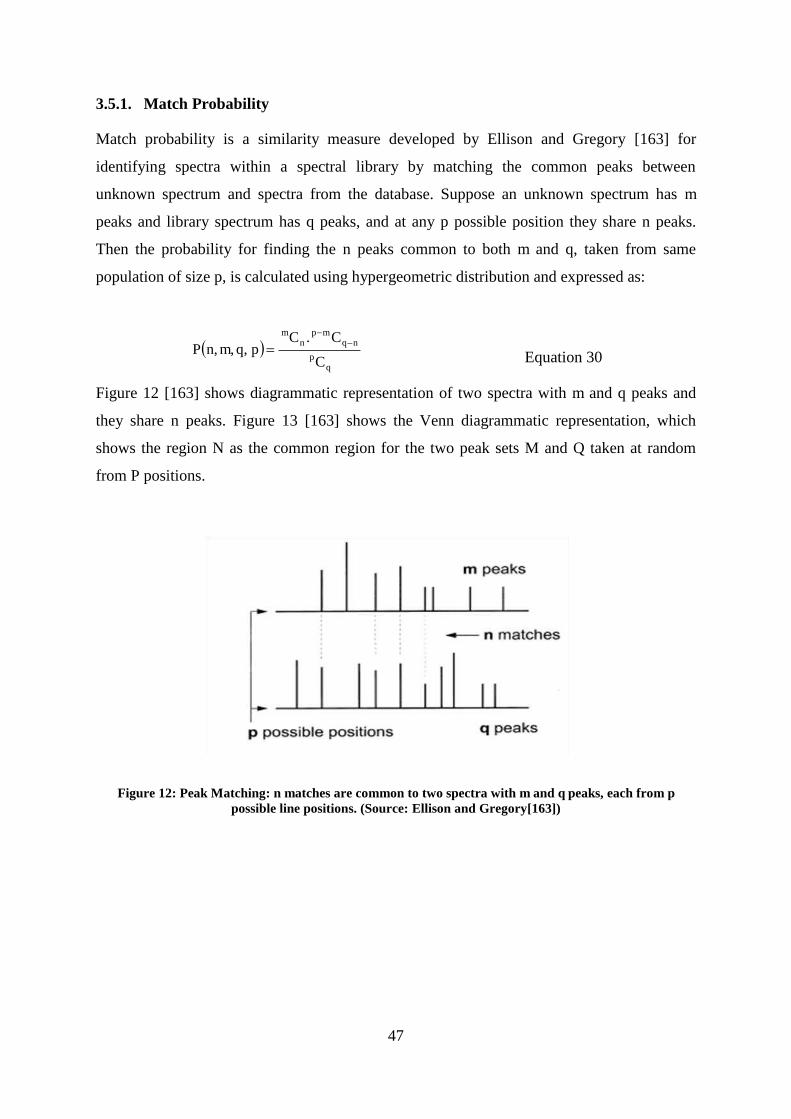
47
3.5.1. Match Probability
Match probability is a similarity measure developed by Ellison and Gregory [163] for
identifying spectra within a spectral library by matching the common peaks between
unknown spectrum and spectra from the database. Suppose an unknown spectrum has m
peaks and library spectrum has q peaks, and at any p possible position they share n peaks.
Then the probability for finding the n peaks common to both m and q, taken from same
population of size p, is calculated using hypergeometric distribution and expressed as:
q
p
nqmp
nm
C
CCpqmnP
.
,,,
Equation 30
Figure 12 [163] shows diagrammatic representation of two spectra with m and q peaks and
they share n peaks. Figure 13 [163] shows the Venn diagrammatic representation, which
shows the region N as the common region for the two peak sets M and Q taken at random
from P positions.
Figure 12: Peak Matching: n matches are common to two spectra with m and q peaks, each from p possible line positions. (Source: Ellison and Gregory[163])

48
Figure 13: Venn diagram for underlying hypergeometric distribution. (Source Ellison and Gregory [163])
They observe that this method yields better search results when an unknown spectrum is
searched against the spectral library than using the simple binomial distribution predictions.
3.5.2. Nonlinear Spectral Similarity Measure
This is a non-linear method for measuring spectral similarity measure between two spectra
[164]. The method not only considers the shape similarity of spectra but also the function of
various absorption features. The adjacent bands in spectrum are usually highly correlated,
which is removed by first projecting the spectral vectors in feature space and applying Kernel
Principal Component Analysis (KPCA). In this method, the kernel function of polar
coordinates is used. Finally, a linear similarity measure is used to find similarity between the
two non-linearly transformed spectra. The method is reported to be effective in spectral
similarity measure [164].
3.5.3. A Spectral Similarity Measure using Bayesian Statistics
This spectral similarity method [165] is based on differentiating subtle differences between
two spectra. These subtle differences mean that the two spectra may overlap quite well in
general except for some local regions. In these local regions, the differences among the
spectra may look insignificant, which may not be the case. Such subtle differences will cause
problems for many spectral search methods. For example, correlation coefficient will give a
similarity index value of approximately 1.0 (or 100%) for these kinds of spectral pairs. This
method transforms the spectral similarity measure into a hypothesis test of the similarities
and differences between the unknown spectra and the spectra from the library. A difference
vectors is defined that denotes the difference between the two spectra and its scalar mean is
used as the statistical variable for the hypothesis test. A threshold is also proposed for the
49
hypothesis that the spectra are different. The Bayesian prior odds ratio is estimated from
several spectra of the same sample. The posterior odds ratio is used to quantity the spectral
similarity measure of the two spectra. They demonstrated the effectiveness of their method on
diffuse reflectance near-infrared spectra of tobacco samples of two formulations and show
that their method can detect subtle differences between the spectra.
3.6. Spectral Similarity Methods Specific for Spectral Data
3.6.1. Spectral Linear Kernel
Spectral Linear Kernel [139] (SLK) is a special similarity metric designed specifically for
computing the spectral similarity between two Raman spectra. The kernel function is
sometimes described as a similarity metric which can be then applied in spectroscopy. This
measure compares two sample spectra and returns a score: the higher this score, the more
similar the two spectra are to each other. This method utilizes information about the spectra
profile such as the presence of peaks or troughs in a particular region. This method not only
takes into consideration the original intensity values at each wavenumber, but also includes
the difference between the intensity at a point and number of its neighbouring points on the
spectrum (called a window). The use of neighbouring points within a window places greater
importance on differences between points sharing the same spectral region than on difference
between points that are far apart on the spectrum. The similarity metric can be expressed as:
Equation 31
where is the similarity value as computed by the SLK, W is the window size that
consists of neighbouring points in a spectra at value i. Figure 14 illustrates the working of
spectral linear kernel.
3.6.2. Weighted Spectral Linear Kernel
The Weighted Spectral Linear Kernel [166] (WSLK) is similar to SLK with a small
modification that it also incorporates the pure spectrum, meaning thereby, it gives more
weights to similarities between spectra in those regions where the corresponding pure
substance has peaks of high magnitude. The similarity metric can be expressed as:

50
Equation 32
where is the intensity of pure substance at wave number i. The value of w is normalized
between 0 and 1. Figure 15 shows the comparison of two spectra using WSLK. The kernel
gives more importance to similarities between two sample spectra that occur in spectral
regions in which strong peaks exist in the pure target spectrum. Similarities in spectral region
that do not overlap with target spectrum peaks are given lower weighting.
Figure 14: Spectral Linear Kernel (Source [139])

51
Figure 15: Comparing two spectra using Weighted Spectral Linear Kernel (Source [139])
3.7. A New Modified Euclidean Spectral Similarity Metric
As mentioned in Section 3.2.4, in spectral library search an unknown spectrum is matched
against a database of pure materials and based on a match score, a list of nearest matches is
produced. The unknown spectrum can be a pure material or a mixture of several pure
materials. If the unknown spectrum is a mixture of several pure materials then the task to find
a nearest match from the database of pure materials becomes very difficult. A mixture may
contain Raman spectra of several pure materials in various proportions which may lead to
either summation of the peaks of individual pure materials or appearance of new peaks at
certain wavelengths in the resulting spectrum of mixture. The convolution of peaks in the
resulting mixture spectrum makes the task of spectral searching more challenging.
The standard Euclidean metric (defined in Section 3.4.1) gives equal importance to peaks of
query spectrum and the spectra in spectral library. However, for computing the similarity of a
mixture against pure materials, this might be undesirable. In this section, we present a new
Modified Euclidean Spectral Similarity Metric that gives weights to the peaks in terms of
penalty or reward according to their absence or presence or the difference in intensities in the

52
unknown spectrum (mixture) and the pure spectra in the spectral library. The performance of
this new similarity method is evaluated relative to other similarity methods in Section 3.8.
Before we explain the new similarity metric, we define some notations to be used in this
section:
Let X be the query spectrum (mixture),
x be the value of intensity of the unknown spectrum at a given wavelength,
A be the pure spectrum from the spectral library, and
a be the value of intensity of the pure spectrum at a given wavelength.
While computing the similarity between an unknown spectrum of mixture against a spectrum
of pure material from the spectral library, at any given wavelength, the following four
scenarios might occur:
1. When the mixture has a peak smaller than the pure substance
If xXaA , and xa
This means that A is (most probably) present in X in some percentage, which means A
bears similarity with X. Therefore this condition should be rewarded i.e. giving
importance to the fact that pure substance is indeed present in the mixture.
2. When the mixture doesn‟t have a peak corresponding to the pure substance
If 0, XaA
X A
X A

53
This means that A is not present in the mixture. Therefore, its occurrence should be
penalized, to accommodate scenarios where the mixture has presence of its constituents.
3. When the mixture has a peak larger than the pure substance
If xXaA , and xa
This condition means that A is present in X in some proportion. So this is a desirable
match. Therefore, no need to penalize it (no reward either).
4. When the mixture has a peak and the corresponding peak in pure substance is absent
If xXA ,0
Here, if the mixture X has a peak, and A has no peak in the same place, then the peak must
come from one of the other constituents in the mixture forming X. However, this is not a
proof that A is definitely not a constituent of the mixture X. In this scenario the best we can
say is that this situation provides no evidence against A being part of the mixture, and only
weak evidence for it. Therefore, it should neither be penalised nor rewarded.
The idea of „penalty‟ means that it is a bad match and the metric should be pushed by a
constant. The „reward‟ means that the match is good and the metric should be reduced. We
penalize by multiplying and reward by dividing with the same constant (the variance of the
mixture).
The Modified Euclidean Spectral Similarity algorithm can be illustrated by following steps:
i. Compute variance of the mixture,
A X
A X

54
ii. For i=1, 2 … N, where N is the number of points in the spectra, Set SqDist=0, Repeat
Step iii.a to iv
iii. Compute distance at every point, as given under:
a. 0 iii XANDXAif , N
i
iiiii
axAXceDis1
2
),(tan
b. 0 iii XANDXAif , N
iiiiii axAXceDis
1
2),(tan
c. Else N
iiiiii axAXceDis
1
2),(tan
iv. iii AXceDisSqDistSqDist ,tan
v. SqDistEuclideanModified _
The Modified Euclidean metric thus capture certain subtleties that need to be considered
while doing a spectral search.
3.8. Comparative Analysis of Spectral Search Methods
In this section we present the measures taken to perform a comparative analysis of various
spectral search algorithms defined in Section 3.4, 3.6 and 3.7. This section details the data
pre-processing steps taken, methodology adopted to compute search performance and the test
strategy formulated for fair comparison of search results. As a representative Raman
spectroscopy dataset, we use a set of spectra from chlorinated and non-chlorinated solvents,
taken from the work of Conroy et al. [167], which is described next.
3.8.1. Description of the Dataset
The chlorinated data set used in our research work is taken from the work of Conroy et al.
[167]. The Raman spectra were recorded on a Labram Infinity (J-Y Horiba) spectrometer. 25
chlorinated and non-chlorinated solvents of different grades were used (see Table 2 ). These
solvents were then mixed in various concentrations to create 225sample mixture of both
chlorinated and non-chlorinated solvents (see Table 3). This exercise was done to try and
replicate possible industrial scenarios.

55
Solvents Grade Solvents Grade
Acetone HPLC Acetophenol* Analytical
Toluene Spectroscopic n-Pentane Analytical
Cyclohexane Analytical & Spectroscopic Xylene Analytical
Acetonitrile Spectroscopic Nitromethane Analytical
2-Propanol Spectroscopic Dimethylformamide Analytical
1,4-Dioxane Analytical & Spectroscopic Nitrobenzene* Analytical
Hexane Analytical Tetrahydrofuran Analytical
1-Butanol Analytical & Spectroscopic Diethyl Ether Analytical
Methyl Alcohol Analytical Petroleum Acetate Analytical
Benzene Analytical Chloroform Analytical & Spectroscopic
Ethyl Acetate Analytical Dichloromethane Analytical & Spectroscopic
Ethanol Analytical 1,1,1-Trichloroethane Analytical & Spectroscopic
Cyclopentane Analytical - -
Table 2: List of chlorinated and non-chlorinated solvents and the various grades used. *Solvents containing fluorescent impurities (Source Conroy et al. [167])

56
Pure
Solvents
Binary
Mixture
Ternary
Mixtures
Quaternary
Mixtures
Quintary
Mixtures Total
Chlorinated 3 96 40 12 0 151
Non-
Chlorinated 22 23 12 10 7 74
Total Number 25 119 52 22 7 225
Table 3: Summary of various chlorinated and non-chlorinated solvent mixtures (Source Conroy et al. [167])
3.8.2. Data Pre-processing
We implemented quadratic polynomial curve fitting for baseline correction. Here a quadratic
polynomial is approximated for each spectrum and then subtracted from the given spectrum
to get corrected baseline. The normalization of baseline corrected spectrum is done using
min-max normalization method described in Section 3.3.1
3.8.3. Methodology for Measuring Search Performance
The performance of search and comparison algorithms is evaluated using the spectral library
search method. In this method an unknown test spectrum (X) is provided by the user as the
input. This spectrum, X, is from a material of known composition but its composition is
hidden for the purposes of testing. This spectrum can either be a pure material or mixture of
two or more materials. The spectrum X will be searched against all the spectra present in the
spectral database. The spectral database consists of spectra of pure substances. The searching
of unknown spectrum against the spectral library is done using a variety of spectral search
algorithms mentioned in Section 3.8.5.
A diagrammatic representation of the Spectral Search method is provided in Figure 16. In the
figure, top ten search results are shown in two different colours. Green colour signifies a
correct search result or the presence of target chemical in the search results, and red colour
signifies an incorrect search result or absence of target chemical in the search results.
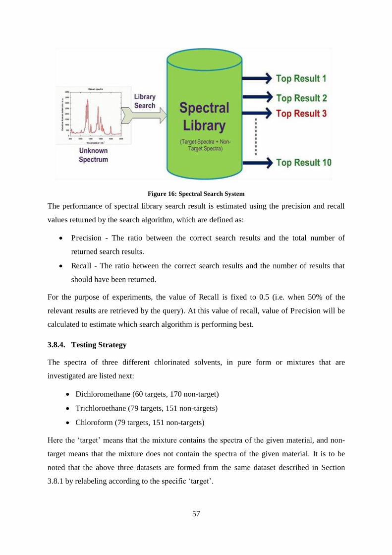
57
Figure 16: Spectral Search System
The performance of spectral library search result is estimated using the precision and recall
values returned by the search algorithm, which are defined as:
Precision - The ratio between the correct search results and the total number of
returned search results.
Recall - The ratio between the correct search results and the number of results that
should have been returned.
For the purpose of experiments, the value of Recall is fixed to 0.5 (i.e. when 50% of the
relevant results are retrieved by the query). At this value of recall, value of Precision will be
calculated to estimate which search algorithm is performing best.
3.8.4. Testing Strategy
The spectra of three different chlorinated solvents, in pure form or mixtures that are
investigated are listed next:
Dichloromethane (60 targets, 170 non-target)
Trichloroethane (79 targets, 151 non-targets)
Chloroform (79 targets, 151 non-targets)
Here the „target‟ means that the mixture contains the spectra of the given material, and non-
target means that the mixture does not contain the spectra of the given material. It is to be
noted that the above three datasets are formed from the same dataset described in Section
3.8.1 by relabeling according to the specific „target‟.

58
To test search accuracy of spectral search algorithms, three separate sets of experiments have
to be executed (for each of the above defined chemical materials). All these experiments have
these common steps:
Randomly Split the target chemical spectra into two parts: 25% for testing the
efficiency of the search algorithm (test set), and 75% to be part of spectral library.
Creating the spectral library by adding to it all the non-target spectra plus 75% of target
spectra.
For every test spectrum i in the test set, do the following,
For every spectral search algorithm j, fix the value of Recall=0.5 (approx.)
Compute the value of jiecision,Pr at this recall value
Compute the average value of jiecision,Pr across all test set (for a particular
spectral search algorithm), to show overall precision of the occurrence of target
chemical when (around) 50% of the target chemical spectra in search results have
been retrieved successfully.
Mathematically, it can be expressed as
Equation 33
Compare values of different search algorithms. An algorithm
with higher value of shall be deemed as better than others at a
fixed value of recall.
3.8.5. Spectral Search Algorithms
The various spectral search algorithms that will be evaluated are as follows:
1. Euclidean metric
2. Modified Euclidean Metric
3. Citiblock Metric
4. Cosine
5. Spectral Linear Kernel (SLK)
6. Weighted Spectral Linear Kernel (WSLK)

59
3.9. Evaluation Relative to Standard Algorithms
The data set to be used for evaluation of spectral search algorithms is presented in Section
3.8.1 and 3.8.4. The search algorithms (see Section 3.8.5) are tested on this dataset and the
value of (at fixed recall) is used as a metric to measure the performance
of these algorithms.
Note: Although the value of recall is set to 0.5, but in computation it is slightly higher. The
reason is that the number of retrieved spectra is always a natural number and cannot be
expressed as a decimal. For example, for the dataset described in Section 3.9.1, the total
number of target spectra to be retrieved by a given query is 45. The threshold here is to
retrieve 50% of the 45 spectra that equals to 22.5 spectra, which is rounded of to 23 spectra
and therefore the recall becomes 511.04523 . The recall values of datasets in Section 3.9.2
and 3.9.3 can be explained in the same way.
The paired t-test [168] is used as statistic to evaluate significant different between average
precision values obtained from search algorithms. The null hypothesis was set so that “the
values of average precision from two search algorithms are same”. The confidence interval is
set to 95% and two-tailed test is employed. If the calculated p-value is lower than this
threshold then we reject the null hypothesis and interpret that the mean values of average
precision from two search algorithms are not same. MS-Excel 2007‟s TTEST function [169]
is used to compute the p-value and determine whether the two average precision have same
mean or not.
3.9.1. Dichloromethane
The details of the Dichloromethane data used for testing the spectral library are as follows:
Total number of Spectra = 230
Number of Targets Spectra = 60
Number of Non-Target Spectra = 170
Number of Test Spectra = 15
Size of Spectral Library = 45 target + 170 Non Target = 215
The results for dichloromethane data set are presented in Table 4.

60
(Dis)similarity Metrics Average Precision (Recall = 0.511) Standard Deviation
Euclidean 0.2194 0.0393
Modified Euclidean 0.2664 0.0480
Citiblock 0.2402 0.0417
Cosine 0.1896 0.0427
SLK 0.1802 0.0152
WSLK 0.2888 0.0305
Table 4: Average Precision Results for Dichloromethane Data
These results of Table 4 are presented graphically in Figure 17.
Figure 17: Average Precision search results for Dichloromethane
It can be observed from Table 4 and Figure 17 that for a recall value of 0.511, WSLK
performed the best with highest average precision rate. The paired t-test shows that WSLK‟s
average precision value is statistically different from rest of the other search algorithms
except Modified Euclidean. Modified Euclidean comes a close second but it is not statistically
0
0.05
0.1
0.15
0.2
0.25
0.3
Euclidean M.Euclidean Citiblock Cosine SLK WSLK
Av
era
ge
Pre
cisi
on
(Dis)similarity Metrics
Dichloromethane

61
much different from WSLK and Citiblock, which comes a close third. The other three search
algorithms perform worse in comparison to these algorithms.
3.9.2. Trichloroethane
The details of Trichloroethane data used for testing the spectral library are as follows:
Total number of Spectra = 230
Number of targets Spectra = 79
Number of Non-target Spectra = 151
Number of Test Spectra = 20
Size of Spectral Library = 59 target + 151 Non Target = 210
The results for trichloroethane data set are presented in Table 5
(Dis)similarity Metrics Average Precision (Recall = 0.508) Standard Deviation
Euclidean 0.2689 0.0208
Modified Euclidean 0.2909 0.0403
Citiblock 0.2920 0.0331
Cosine 0.2643 0.0405
SLK 0.2860 0.0559
WSLK 0.3725 0.0574
Table 5: Average Precision results for Trichloroethane Data
The above tabular results can be visualized graphically in Figure 18.

62
Figure 18: Average Precision search results for Trichloroethane
Table 5 and Figure 18 shows that, for a fixed recall value of 0.508, WSLK metrics performs
the best for the Trichloroethane data with highest average precision. The paired t-test shows
that it is statistically different from the average precision values obtained from other
algorithms. Modified Euclidean and Citiblock comes close second and third with no statistical
difference among them. Both of them are not statistically significantly different from SLK
either. Therefore it is difficult to say that SLK performs worse than them. Cosine and
Euclidean metric performs worst with no statistical difference among them.
3.9.3. Chloroform
The details of Chloroform dataset used for testing the spectral library are as follows:
The data description for testing the spectral library is as under:
Total number of Spectra = 230
Number of targets Spectra = 79
Number of Non-target Spectra = 151
Number of Test Spectra = 20
Size of Spectral Library = 59 target + 151 Non Target = 210
The results for chloroform data set are presented in Table 6
0
0.05
0.1
0.15
0.2
0.25
0.3
0.35
0.4
Euclidean M.Euclidean Citiblock Cosine SLK WSLK
Av
era
ge
Pre
cisi
on
(Dis)similarity Metrics
Trichloroethane

63
(Dis)similarity Metrics Average Precision (Recall = 0.508) Standard Deviation
Euclidean 0.2513 0.0174
Modified Euclidean 0.2718 0.0142
Citiblock 0.2661 0.0177
Cosine 0.2468 0.0166
SLK 0.2710 0.0196
WSLK 0.9586 0.0851
Table 6. Average Precision results for Chloroform Data
These tabular results are shown graphically in Figure 19.
Figure 19: Average Precision search results for Chloroform
From Table 6 and Figure 19, it can be seen that WSLK performed with much superior average
precision rate (0.9586) for fixed recall of 0.58. The paired t-test also suggests that it is
statistically different from other search algorithms. Modified Euclidean and SLK come second
and very close to each other with no statistical difference in the means. Both of them also do
not have statistical difference in their means when compared with Citiblock, therefore, it
0
0.2
0.4
0.6
0.8
1
Euclidean M.Euclidean Citiblock Cosine SLK WSLK
Av
era
ge
Pre
cisi
on
(Dis)similarity Metrics
Chloroform

64
cannot be interpreted to perform worse than them. Euclidean and Cosine performs the worst
and their means are statistically same using paired t-test.
3.9.4. Evaluation of Spectral Search Algorithms
The evaluation is based on the best three search algorithms for the chlorinated solvent test
data set. The results are presented in Figure 20.
Data Sets Best Search Algorithms
First Second Third
Dicholormethane WSLK Modified Euclidean Citiblock
Trichloroethane WSLK Modified Euclidean / Citiblock SLK
Chloroform WSLK Modified Euclidean / SLK Citiblock
Figure 20: Overall Evaluation of Best 3 Spectral Search Algorithms on Chlorinated Solvent data
It can be seen that WSLK similarity measure gives consistently the best average precision rate
for all the three chlorinated solvent data considered. Modified Euclidean dissimilarity
measure emerged as the second best spectral search algorithm consistently for the three
chlorinated solvent data set. The next best choice for the choice of spectral search algorithm
is SLK and Citiblock. The paired t-test shows that some of the spectral algorithms‟s average
precision values may not be significantly different than others, however Euclidean metric
perform worst in almost all the cases.
It can be concluded that for the chlorinated solvent data, WSLK is the overall best of the
similarity metrics that have been evaluated. The reason for the superior performance of
WSLK lies in the fact that it gives importance to those regions in a spectrum where the pure
substance has peaks and also the points in the neighbourhood at any point in a spectrum.
Modified Euclidean came the modest second among spectral search algorithms we evaluated.
The reason for its good and consistent performance is that it does not give equal importance
to peaks of an unknown material to be searched in spectral library (unlike Euclidean metric),
rather it rewards or penalizes the occurrence or absence of peaks in conjunction with
calculating Euclidean distance as well. SLK and Citiblock are the next close choices. SLK‟s
strength lies in the fact that it considers not only a portion of spectrum to be searched against

65
spectral library but also its nearby points to capture a general similarity spread across a
localized region. The better performance of Citiblock in comparison to other standard spectral
search methods might be due to the presence of sharp peaks in the unknown spectrum.
Standard Euclidean search method never gave good results in comparison to other spectral
search algorithms. Cosine metric gave the worse results in all the three chlorinated solvents
data.
This study shows that in spectroscopic applications, standard spectral search algorithms are a
good starting point to develop an understanding about the spectral search mechanism.
However, it does not guarantee the best spectral library search results. The reason is that they
do not embody any domain specific insight into the data. Therefore, from our experiments we
deduce that spectral search accuracy can be improved by devising customized non-standard
spectral search algorithms that are more specific to spectroscopic data and capture more
information that traditional spectral search algorithms might not.

66
Chapter 4
One-class K-Nearest Neighbour
Approach based on Kernels
The K-nearest neighbour (KNN) [76] is a standard approach for solving multi class
classification problems. It has been modified to tackle the problem of one-class classification
by Tax in his thesis [2]. Various other researchers have also presented variants of one-class
nearest neighbour approach (see Section 4.3). In this chapter we present modification on the
standard one-class KNN based algorithms presented by Tax. We incorporate the use of kernel
functions as distance metric instead of the conventional Euclidean based distance metrics. In
a traditional KNN classifier, the k nearest neighbours‟ class labels are used to decide the class
allotment of a test case. We extend that approach by not only considering j nearest
neighbours, but their k nearest neighbours also and an averaged decision is taken to allocate a
class to a test sample.
4.1. Kernel as Distance Metric
The conventional nearest neighbour (NN) classifier uses Euclidean measure as a distance
metric to compute similarity between two vectors. This distance metric can be redefined by
incorporating the „kernel approach‟ and applied to conventional NN classifier [170]. The idea
of applying a kernel is to transform the data into high dimensional feature space by
performing a nonlinear mapping and then try to define a classification boundary around it in
that space. For further details on „kernel approach‟, refer to Section 2.4.1.
As described by Yu et al. [170], suppose an n dimensional vector is transformed to m
dimensional feature space using some non-linear mapping:
Here is the original n dimensional space and is the transformed m dimensional feature
space. x is a vector in space and is the corresponding vector is space . is a non

67
linear mapping that transforms the vector in original space to a high dimensional space .
And are the mapping functions.
A kernel function, K(...), can be expressed as inner dot product of the vector in new
transformed space without actually carrying out the mapping . Mathematically it can be
written as: Equation 34
where denotes the dot product of and . The popular kernel functions
that are used commonly are [29] (also see Section 2.4.1):
Polynomial kernel dyxyxK ,1, , where d is the degree of
the polynomial
Radial Basis Function (RBF) 222/exp, yxyxK
, where is
width of the kernel
Sigmoidal yxyxK .tanh, , with gain and
offset
The parameters p, , and are all adjustable to tune the suitability of a kernel function.
As described by Yu et al. [170], the norm distance between two vectors can be expressed as: Equation 35
By decomposing of into inner products and substitution of Equation 34 for the inner products we get Equation 36
Or it can be simplified further as: Equation 37
where is the distance metric between vectors x and y in the kernel space.
4.2. Kernel-based KNN Classifiers
The „kernel approach‟ has been used by various researchers to implement different flavours
of NN-based classifier. Yu et al. [170] applied the „kernel approach‟ to modify the norm
distance metric and present the Kernel KNN classifier. They proved that the conventional NN

68
classifier is a special case of the Kernel NN when radial basis kernel or polynomial kernel
with degree 1 is chosen. They therefore argue that the Kernel KNN will not perform worse
than conventional NN. Also, since the distance metric calculation process is only altered, the
computation time of the Kernel NN and the conventional NN shall remain comparable. They
show their results on BUPA Liver Disorder data set [50] and US Postal Service data. Their
experimental results on Kernel KNN are better than conventional KNN classifiers and can
compete with SVM.
Peng et al. [171] present a quasiconformal kernel method for nearest neighbour classification.
In traditional NN methods, when the data becomes sparse in high dimensional space, to find
nearest neighbourhood one need to look far away from the test sample that may induce severe
bias. Their method produces neighbourhoods where the class conditional probabilities tend to
be homogenous. This is done by employing quasiconformal kernels as distance metric which tend to
move the samples closer to the test example if the class posterior probabilities are similar. Similarly, if
the class posterior probabilities of samples are different from the test example, they are moved farther
away from it. The resulting effect is to create neighbourhood with homogenous class conditional
probabilities. Their experimental results on UCI datasets [50] demonstrate that the algorithm
can potentially improve the performance of KNN in some classification and data mining
problems.
Daqi and Jie [172] propose a Kernel Fisher Discriminant used with KNN algorithm to solve
large scale learning problems. Their main idea is to first, to decompose a large scale multi-
class classification problem into multiple two class problems. Secondly, the samples in each
class of the two class problems are covered by hyper-dimensional spheres with different
sizes, and repeat the process until all of them are included within hyper-spheres of different
sizes. Such spheres can be considered as new prototypes and they are relatively less than the
original number of samples. Finally, if the Euclidean distance between a test sample and the
surface of the sphere of a class is smallest, the sample is assigned the class of the sphere. This
kind of kernel KNN classifier only needs to store a small proportion of samples in the form of
prototypes. Their results on USPS and letter recognition data show that their method has
higher classification accuracy than the standard classification methods they compared with.
4.3. One-class KNN Classifiers
Tax [2] presents a one-class nearest neighbour method, called nearest neighbour description
(NN-d). In NN-d, a test object z is accepted when its local density is larger or equal to the

69
local density of its nearest neighbour in the training set (for detail refer to Section 2.4.3.4).
Munroe and Madden [137] extends the idea of one-class KNN to tackle the recognition of
vehicles using a set of features extracted from their frontal view and presented high accuracy
of classification. They also implemented multi class classifiers to compare their method.
They comment that it is not reasonable to draw direct comparisons between the results of the
multi-class and single-class classifiers, because the experimental methodology and
underlying assumptions are quite different. They also make a note that the performance of
multi class classifier could be made arbitrarily worse by adding those vehicle types to the test
set that do not appear in the training set, however, since one-class classifiers can represent the
concept „none of the above‟, their performance should not deteriorate in these conditions.
Cabral et al. [173] propose a one-class nearest neighbour data description using the concept
of structural risk minimization. KNN suffers with the drawback of storing all training
samples as prototypes that would be used to classify an unseen sample. Their paper is based
on the idea of removing redundant samples from the training set, thereby obtaining a compact
representation aiming at improving generalization performance of the classifier. Their results
on artificial and UCI datasets [50] have shown improved performance than the NN-d
classifiers. Their method also achieved considerable reduction in number of stored
prototypes. Cabral et al. [174] extended their work and presented another approach where
they not only consider the 1 NN but all the k-nearest neighbours and arrive at a decision
based on majority voting. In their experiments they observe that K nearest neighbour version
of their classifier outperforms the 1 NN and is better than NN-d algorithms. They tested their
algorithm on artificial data, biomedical data [37] and data from the UCI repository [50].
Gesù et al. [175] presents a one-class KNN and tested it on synthetic data that simulate
microarray data for the identification of nucleosomes and linker regions across DNA. They
presented a decision rule to classify an unknown sample X as:
Equation 38
where is the training set for the patterns P representing positive instance, is the
dissimilarity function between patterns. Also, j=1 means that x is positive. The above rule
translates to that if there are at least K patterns in dissimilar from x at most , then x is
classified as a positive pattern, otherwise it is classified as negative. This KNN model
depends on parameters K and and their values are chosen by using optimization methods.
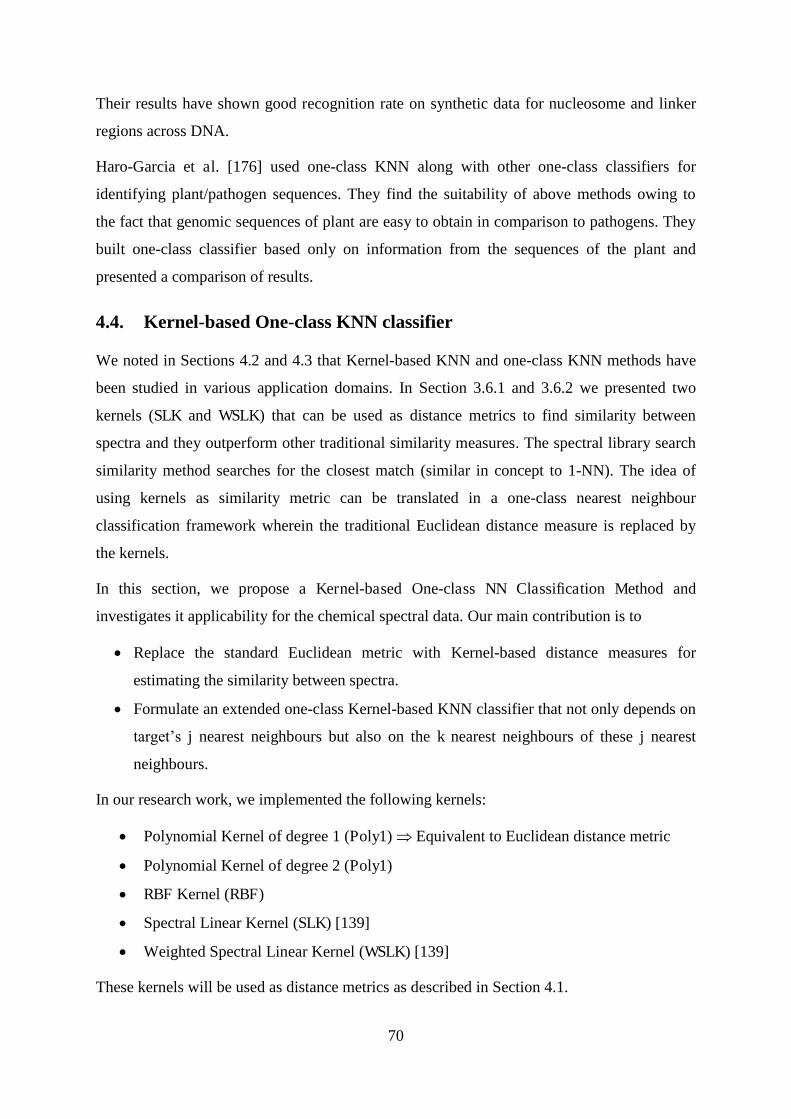
70
Their results have shown good recognition rate on synthetic data for nucleosome and linker
regions across DNA.
Haro-Garcia et al. [176] used one-class KNN along with other one-class classifiers for
identifying plant/pathogen sequences. They find the suitability of above methods owing to
the fact that genomic sequences of plant are easy to obtain in comparison to pathogens. They
built one-class classifier based only on information from the sequences of the plant and
presented a comparison of results.
4.4. Kernel-based One-class KNN classifier
We noted in Sections 4.2 and 4.3 that Kernel-based KNN and one-class KNN methods have
been studied in various application domains. In Section 3.6.1 and 3.6.2 we presented two
kernels (SLK and WSLK) that can be used as distance metrics to find similarity between
spectra and they outperform other traditional similarity measures. The spectral library search
similarity method searches for the closest match (similar in concept to 1-NN). The idea of
using kernels as similarity metric can be translated in a one-class nearest neighbour
classification framework wherein the traditional Euclidean distance measure is replaced by
the kernels.
In this section, we propose a Kernel-based One-class NN Classification Method and
investigates it applicability for the chemical spectral data. Our main contribution is to
Replace the standard Euclidean metric with Kernel-based distance measures for
estimating the similarity between spectra.
Formulate an extended one-class Kernel-based KNN classifier that not only depends on
target‟s j nearest neighbours but also on the k nearest neighbours of these j nearest
neighbours.
In our research work, we implemented the following kernels:
Polynomial Kernel of degree 1 (Poly1) Equivalent to Euclidean distance metric
Polynomial Kernel of degree 2 (Poly1)
RBF Kernel (RBF)
Spectral Linear Kernel (SLK) [139]
Weighted Spectral Linear Kernel (WSLK) [139]
These kernels will be used as distance metrics as described in Section 4.1.
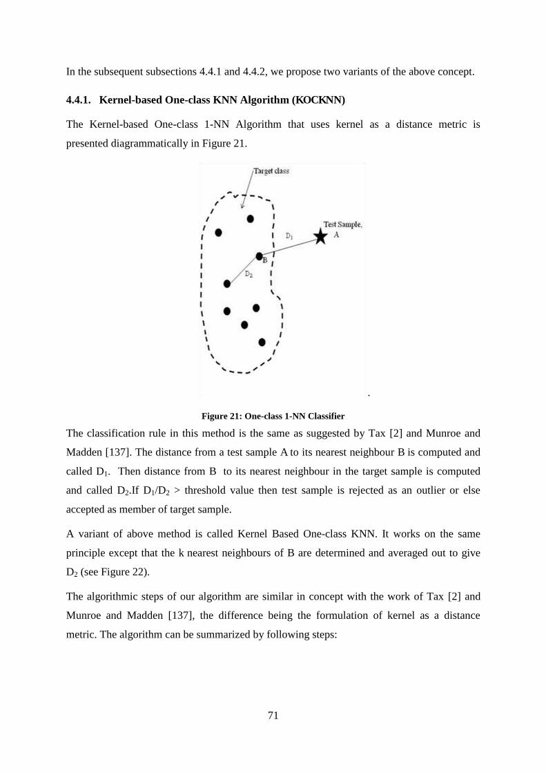
71
In the subsequent subsections 4.4.1 and 4.4.2, we propose two variants of the above concept.
4.4.1. Kernel-based One-class KNN Algorithm (KOCKNN)
The Kernel-based One-class 1-NN Algorithm that uses kernel as a distance metric is
presented diagrammatically in Figure 21.
.
Figure 21: One-class 1-NN Classifier
The classification rule in this method is the same as suggested by Tax [2] and Munroe and
Madden [137]. The distance from a test sample A to its nearest neighbour B is computed and
called D1. Then distance from B to its nearest neighbour in the target sample is computed
and called D2.If D1/D2 > threshold value then test sample is rejected as an outlier or else
accepted as member of target sample.
A variant of above method is called Kernel Based One-class KNN. It works on the same
principle except that the k nearest neighbours of B are determined and averaged out to give
D2 (see Figure 22).
The algorithmic steps of our algorithm are similar in concept with the work of Tax [2] and
Munroe and Madden [137], the difference being the formulation of kernel as a distance
metric. The algorithm can be summarized by following steps:
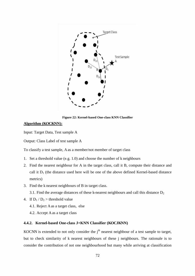
72
Figure 22: Kernel-based One-class KNN Classifier
Algorithm (KOCKNN):
Input: Target Data, Test sample A
Output: Class Label of test sample A
To classify a test sample, A as a member/not member of target class
1. Set a threshold value (e.g. 1.0) and choose the number of k neighbours
2. Find the nearest neighbour for A in the target class, call it B, compute their distance and
call it D1 (the distance used here will be one of the above defined Kernel-based distance
metrics)
3. Find the k nearest neighbours of B in target class.
3.1. Find the average distances of these k-nearest neighbours and call this distance D2
4. If D1 / D2 > threshold value
4.1. Reject A as a target class, else
4.2. Accept A as a target class
4.4.2. Kernel-based One-class J+KNN Classifier (KOCJKNN)
KOCNN is extended to not only consider the jth nearest neighbour of a test sample to target,
but to check similarity of k nearest neighbours of these j neighbours. The rationale is to
consider the contribution of not one neighbourhood but many while arriving at classification

73
decision. The distance metric used will be based on kernels rather than Euclidean. In this
method, first the j nearest neighbours of a test sample in target class are computed, then the k
nearest neighbours of these j neighbours are computed in the target class and averaged out
(See Figure 23). The overall results obtained for these j neighbours can be arrived at by using
majority voting rule.
Figure 23: Kernel-based One-class J+KNN Classifier
The algorithmic steps are described below:
Algorithm (KOCJKNN):
Input: Target Data, Test sample A
Output: Class Label of test sample A
To classify a test sample, A as a member/not member of target class
1. Set a threshold value (e.g. 1.0), choose the number of j and k neighbours, set counter
accept to zero (this counter will keep the number of acceptance of test sample as member
of target class)

74
2. Find the j nearest neighbours of the test sample A in the target class, call it , and compute their distance from A and call it . (the distance used here will
be one of the above defined Kernel-based distance metrics)
3. For every j nearest neighbour (i=1,2,...j), repeat Step 4 to 5
4. Find k nearest neighbours for Bj in the target class, call it , compute their
distance from Bj and call this distance (the distance used here will be one
of the above defined Kernel-based distance metrics)
5. Find the average distances of the k nearest neighbours for Bj in the target class and call
this distance D2
5.1. If D1j / D2 < threshold value
5.2. Increase the counter accept
6. If accept ≥ Ceiling(j/2) [majority voting rule], then
6.1. Accept A as a member of target class, else
6.2. Reject A as a member of target class
Note: When j is set to 1 and k is set to 1in KOCJKNN, it condenses to Kernel-based 1-NN,
similarly when j is set to 1 it condenses to KOCKNN
In the next chapter we present classification results on the chlorinated solvents data using
Kernel-based One-class nearest approaches proposed above.

75
Chapter 5
Experimentation and Results
This chapter describes the experimentation, results obtained, and their analysis on the
chlorinated solvent data set, for the application of identifying chlorinated solvents using the
kernel as distance metric applied to one-class nearest neighbour classification. At the end of
the chapter, conclusions are presented and future directions for this research are discussed.
5.1. Experimentations
5.1.1. Dataset
The chlorinated solvent data is used to evaluate the performance of Kernel-based One-class
nearest neighbour classifier. This data set is described in Section 3.8.1.
5.1.2. Setting Parameters
In the experiment KOCJKNN classifier (see Section 4.4.2) is implemented with values of j
nearest neighbours set to 1, 3 and 5 and k nearest neighbours set to 1, 3, 5 and 7. This
exercise is done to study the effect of varying number of nearest neighbours to the test sample
in the target class and its nearest neighbours. The value of threshold to accept or reject a test
sample as member of target or outlier class is set to 1. For the first 3 datasets, five one-class
kernels were implemented as mentioned in Section 4.4. A fourth dataset is also created from
the three main chlorinated solvent data sets, called ChlroinatedOrNot. This data contains the
spectra of all those substances that contain one or more of the chlorinated solvents (in any of
the three chlorinated solvent data sets) as one of its constituent. For this data, WSLK is not
implemented as it only works for the case when we have the spectra of pure substances. As
mentioned in Section 3.6.2, WSLK computes similarity between two spectra (at given
wavenumber) by computing similarity between their peaks in a neighbourhood with
providing more weights at positions where the corresponding pure substance has a peak of
higher magnitude. Since ChlroinatedOrNot only contains information about whether
chlorinated solvent is present or not and no information about individual pure chlorinated
solvents, WSLK is omitted from implementation for this dataset. For kernels Poly1 and Poly2

76
default settings are used. For RBF kernel, kernel width of 1 is chosen. For SLK and WSLK the
window size (neighbourhood) of 3 is used in the experiment.
5.1.3. Splitting into Training and Testing Sets
To perform an experiment, we randomly divide a dataset (i.e. target class) into 67% to form a
training set and the remaining 33% to form a test set. An outlier dataset (equal to the number
of test set samples) is also constructed by randomly selecting samples from the non-target
class. This process is repeated 10 times and the average error is reported. The numbers of
test set and outlier samples are kept equal for fair estimation of errors.
5.2. Performance Evaluation
The performance of the KOCJKNN is measured by first computing accuracy, which can be
expressed as:
jectAcceptjectAccept
jectAccept
OOTT
OTaccuracy
ReRe
Re
Equation 39
where
AcceptT is the number of targets accepted as targets
jectTRe is the number of targets rejected as outliers
AcceptO is the number of outliers accepted as targets
jectORe is the number of outliers rejected as outliers
Error is calculated as:
accuracyerror 1 Equation 40
Error is used as performance metric to evaluate different kernels used as distance metric. In
the following tables any entry in a cell can be read as average error for a particular Kernel
(the row) and (j,k) nearest neighbour (column). The values in grey and bold emphasize the
best results obtained.

77
5.2.1. Dichloromethane
Kernels Nearest Neighbour (j,k)
1,1 1,3 1,5 1,7
3,1 3,3 3,5 3,7
5,1 5,3 5,5 5,7
Poly1 0.275 0.178 0.173 0.295 0.437 0.308 0.27 0.293 0.487 0.397 0.3 0.305
Poly2 0.27 0.2 0.175 0.283 0.437 0.315 0.265 0.283 0.487 0.385 0.29 0.285
RBF 0.275 0.125 0.097 0.18 0.462 0.31 0.235 0.222 0.515 0.408 0.285 0.245
SLK 0.305 0.185 0.173 0.25 0.445 0.32 0.28 0.252 0.482 0.4 0.308 0.265
WSLK 0.272 0.205 0.283 0.327 0.392 0.22 0.298 0.355 0.497 0.335 0.332 0.342
Table 7: One-class Kernel-based j+kNN results for Dichloromethane Data
The above tabular results can be presented in graphical form as shown in Figure 24 (a), (b)
and (c).
(a)
0
0.05
0.1
0.15
0.2
0.25
0.3
0.35
0.4
0.45
0.5
0.55
1,1 1,3 1,5 1,7
Av
era
ge
Err
or
Nearest Neighbour (j,k)
Poly1
Poly2
RBF
SLK
WSLK

78
(b)
(c)
Figure 24: Effect of varying j and k Nearest Neighbours on different Kernels for Dichloromethane Data
Table 7 suggests that the lowest value of error is obtained for j=1 and k=5 for the one-class
RBF Kernel. Figure 24 shows the effect of increasing k neighbours with fixed value of j.
When the value of k is increased error initially decreases but after certain value of k it tends to
increase. A different view is to look at error values by fixing k neighbours and increasing j.
Doing so, in general, tend to increase error for almost all the kernels.
0
0.05
0.1
0.15
0.2
0.25
0.3
0.35
0.4
0.45
0.5
0.55
3,1 3,3 3,5 3,7
Av
era
ge
Err
or
Nearest Neighbour (j,k)
Poly1
Poly2
RBF
SLK
WSLK
0
0.05
0.1
0.15
0.2
0.25
0.3
0.35
0.4
0.45
0.5
0.55
5,1 5,3 5,5 5,7
Av
era
ge
Err
or
Nearest Neighbour (j,k)
Poly1
Poly2
RBF
SLK
WSLK

79
5.2.2. Trichloroethane
Table 8 shows the KOCJKNN results for Trichloroethane data.
Kernels Nearest Neighbours (j,k)
1,1 1,3 1,5 1,7
3,1 3,3 3,5 3,7
5,1 5,3 5,5 5,7
Poly1 0.256 0.198 0.222 0.322 0.374 0.267 0.257 0.322 0.485 0.374 0.339 0.335
Poly2 0.267 0.198 0.23 0.326 0.374 0.278 0.263 0.319 0.485 0.376 0.346 0.354
RBF 0.256 0.154 0.139 0.178 0.426 0.283 0.207 0.204 0.55 0.435 0.326 0.267
SLK 0.276 0.207 0.239 0.333 0.391 0.281 0.28 0.331 0.481 0.363 0.331 0.335
WSLK 0.265 0.209 0.309 0.398 0.411 0.28 0.293 0.367 0.487 0.394 0.326 0.346
Table 8: One-class Kernel-based j+kNN results for Trichloroethane
Figure 25 (a), (b) and (c) presents the above results in graphical form.
(a)
0
0.05
0.1
0.15
0.2
0.25
0.3
0.35
0.4
0.45
0.5
0.55
1,1 1,3 1,5 1,7
Av
era
ge
Err
or
Nearest Neighbour (j,k)
Poly1
Poly2
RBF
SLK
WSLK
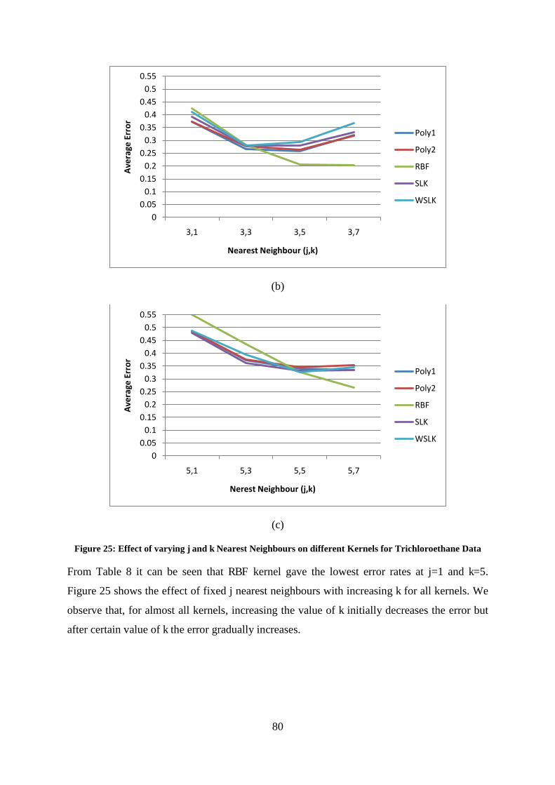
80
(b)
(c)
Figure 25: Effect of varying j and k Nearest Neighbours on different Kernels for Trichloroethane Data
From Table 8 it can be seen that RBF kernel gave the lowest error rates at j=1 and k=5.
Figure 25 shows the effect of fixed j nearest neighbours with increasing k for all kernels. We
observe that, for almost all kernels, increasing the value of k initially decreases the error but
after certain value of k the error gradually increases.
0
0.05
0.1
0.15
0.2
0.25
0.3
0.35
0.4
0.45
0.5
0.55
3,1 3,3 3,5 3,7
Av
era
ge
Err
or
Nearest Neighbour (j,k)
Poly1
Poly2
RBF
SLK
WSLK
0
0.05
0.1
0.15
0.2
0.25
0.3
0.35
0.4
0.45
0.5
0.55
5,1 5,3 5,5 5,7
Av
era
ge
Err
or
Nerest Neighbour (j,k)
Poly1
Poly2
RBF
SLK
WSLK

81
5.2.3. Chloroform
The classification results of KOCJKNN for chloroform data are shown in Table 9
Kernels Nearest Neighbour (j,k)
1,1 1,3 1,5 1,7
3,1 3,3 3,5 3,7
5,1 5,3 5,5 5,7
Poly1 0.287 0.22 0.243 0.333 0.411 0.328 0.296 0.339 0.48 0.385 0.35 0.363
Poly2 0.278 0.222 0.248 0.328 0.411 0.328 0.298 0.331 0.483 0.389 0.348 0.361
RBF 0.287 0.181 0.143 0.198 0.472 0.341 0.25 0.263 0.572 0.45 0.346 0.33
SLK 0.259 0.211 0.237 0.317 0.406 0.32 0.289 0.343 0.481 0.374 0.341 0.35
WSLK 0.287 0.22 0.243 0.333 0.411 0.328 0.296 0.339 0.48 0.385 0.35 0.363
Table 9: One-class Kernel-based j+kNN results for Chloroform Data
These tabular results are presented graphically in Figure 26 (a), (b) and (c)
(a)
0
0.05
0.1
0.15
0.2
0.25
0.3
0.35
0.4
0.45
0.5
0.55
1,1 1,3 1,5 1,7
Av
era
ge
Err
or
Nearest Neighbour (j,k)
Poly1
Poly2
RBF
SLK
WSLK

82
(b)
(c)
Figure 26: Effect of varying j and k Nearest Neighbours on different Kernels for Chloroform Data
It can be seen from Table 9 that RBF kernel gave the lowest error rate at j=1 and k=5. Figure
26 shows that for fixed j neighbours and increasing k, the value of error initially reduces but
as k increases, the error also increases. This trend is similar for all kernels.
0
0.05
0.1
0.15
0.2
0.25
0.3
0.35
0.4
0.45
0.5
0.55
3,1 3,3 3,5 3,7
Av
era
ge
Err
or
Nearest Neighbor (j,k)
Poly1
Poly2
RBF
SLK
WSLK
0
0.05
0.1
0.15
0.2
0.25
0.3
0.35
0.4
0.45
0.5
0.55
0.6
5,1 5,3 5,5 5,7
Av
era
ge
Err
or
Nearest Neighbour (j,k)
Poly1
Poly2
RBF
SLK
WSLK

83
5.2.4. ChlorinatedOrNot
The classification results for ChlroinatedOrNot using KOCJKNN are shown in Table 10.
Kernels Nearest Neighbours (k,j)
1,1 1,3 1,5 1,7
3,1 3,3 3,5 3,7
5,1 5,3 5,5 5,7
Poly1 0.236 0.141 0.112 0.1 0.399 0.271 0.209 0.177 0.479 0.378 0.306 0.251
Poly2 0.23 0.14 0.119 0.111 0.396 0.278 0.214 0.174 0.474 0.385 0.302 0.253
RBF 0.236 0.124 0.079 0.059 0.41 0.275 0.2 0.162 0.491 0.387 0.308 0.249
SLK 0.238 0.151 0.123 0.112 0.407 0.287 0.219 0.192 0.477 0.382 0.308 0.265
Table 10: One-class Kernel-based j+kNN results for ChlorinatedOrNot
The above tabular results are presented in graphical form in Figure 27 (a), (b) and (c)
(a)
0
0.05
0.1
0.15
0.2
0.25
0.3
0.35
0.4
0.45
0.5
0.55
1,1 1,3 1,5 1,7
Av
era
ge
Err
or
Nearest Neighbour (j,k)
Poly1
Poly2
RBF
SLK

84
(b)
(c)
Figure 27: Effect of varying j and k Nearest Neighbours on different Kernels for ChlorintedOrNot data
Table 10 shows the results of ChlroinatedOrNot data set. The lowest value of error is
obtained with RBF kernel for j=1 and k=7. Figure 27 shows the effect of fixed j neighbours
with increasing value of k neighbours. As the value of k is increased the error shows a
decreasing trend for all kernels with RBF kernel giving the lowest error rates. Alternatively, it
can also be observed from Table 10 that by fixing k neighbours and increasing j neighbours,
in all kernels, the error increases. The error rates for this dataset are very low in comparison
to other three chlorinated solvent datasets, because here the task is much simpler to find only
0
0.05
0.1
0.15
0.2
0.25
0.3
0.35
0.4
0.45
0.5
0.55
3,1 3,3 3,5 3,7
Av
era
ge
Err
or
Nearest Neighbour (j,k)
Poly1
Poly2
RBF
SLK
0
0.05
0.1
0.15
0.2
0.25
0.3
0.35
0.4
0.45
0.5
0.55
5,1 5,3 5,5 5,7
Av
era
ge
Err
or
Nearest Neighbour (j,k)
Poly1
Poly2
RBF
SLK

85
the presence or absence of any chlorinated solvent in a mixture and not individual chlorinated
solvents.
5.2.5. Analysis of Results
We present our analysis of results based on the following criteria:
Increasing the number of k nearest neighbours
From Figure 24, Figure 25, Figure 26 and Figure 27 we observe a common trend that for any
given j nearest neighbours (for almost all kernels), increasing the value of k nearest
neighbour decreases the error rates till a particular value after which it error tends to increase.
This is due to the fact that some of the nearest neighbours are quite close to each other,
however when the number of neighbours are increased the classifier finds far away samples
and this leads to decrease in accuracy.
Increasing the number of j nearest neighbours
From Figure 24, Figure 25, Figure 26 and Figure 27 we observe that for any given kernel and
k nearest neighbour, increasing j nearest neighbours increases the classification error. This
trend is common almost all the data. The reason for this is that the classifier finds nearest
neighbours that are farther away and lead to bad classification results.
On Using Different Kernels
From Table 7, Table 8, Table 9 and Table 10 we observe that for any given k and j nearest
neighbours, One-class RBF Kernel gave the lowest error rates for all the four datasets studied.
By looking at the overall results, we can infer that RBF Kernel when used as distance metric
for implementing KOCJKNN gives the lowest values of errors at j=1 and k=5 or k=7. This
experiment show that a one-class KOCJKNN approach performs better when j=1. Increasing
the value of j neighbours is detrimental for this data set‟s classification accuracy. However
increasing the value of k nearest neighbours to a certain limit may boost the accuracy. We
also deduce that for KOCJKNN classifier, RBF Kernel is much better in performance in
comparison to the Polynomial Kernel of degree 1 (which is equivalent to Euclidean metric)
and other kernels considered. In all the chlorinated datasets studied, only the RBF Kernel
performs significantly better than other kernels. In fact, the quadratic polynomial and spectral
kernels perform no better than the linear kernel which is directly equivalent to the standard
Euclidean metric. Moreover, the spectral kernels that give significantly better performance in

86
the spectral search setting in comparison to Euclidean metric, do not perform any better than
it in the one-class KNN setting.
5.2.6. Effect of Varying Kernel Width in RBF Kernel
In Section 5.2.5 we observe that RBF kernel (on default setting) suits the most as a distance
metric in the implementation of One-class Nearest Neighbour classifier for the chlorinated
solvent data set. To study the effect of varying width of RBF kernel we extended our
experiment and results are shown below.
In the following figures RBF1, RBF5, RBF25 and RBF100 corresponds to RBF kernel with
width, =1, 5, 25 and 100.
Figure 28: RBF Kernel with different widths for Dichloromethane
0
0.05
0.1
0.15
0.2
0.25
0.3
0.35
0.4
0.45
0.5
0.55
0.6
1,1 1,3 1,5 1,7 3,1 3,3 3,5 3,7 5,1 5,3 5,5 5,7
Av
era
ge
Err
or
Nearest Neighbour (j,k)
Dichloromethane
RBF1
RBF5
RBF25
RBF100

87
Figure 29: RBF Kernel with different widths for Trichloroethane
Figure 30: RBF Kernel with different widths for Chloroform
0
0.05
0.1
0.15
0.2
0.25
0.3
0.35
0.4
0.45
0.5
0.55
0.6
1,1 1,3 1,5 1,7 3,1 3,3 3,5 3,7 5,1 5,3 5,5 5,7
Av
era
ge
Err
or
Nearest Neighbour (j,k)
Trichloroethane
RBF1
RBF5
RBF25
RBF100
0
0.05
0.1
0.15
0.2
0.25
0.3
0.35
0.4
0.45
0.5
0.55
0.6
1,1 1,3 1,5 1,7 3,1 3,3 3,5 3,7 5,1 5,3 5,5 5,7
Av
era
ge
Err
or
Nearest Neighbour (j,k)
Chloroform
RBF1
RBF5
RBF25
RBF100

88
Figure 31: RBF Kernel with different widths for ChlorinatedORnot
The same inferences can be drawn by increasing k and j nearest neighbours. The best results
came when j=1 and k=5 or 7. An important point to note is that increasing the kernel width
does not necessarily improves the error rates. In fact, most of the time kernel width, =1 gave
the lowest error rates. This behaviour may be because the chlorinated solvent data is dense in
localized regions and beyond that it gets sparse.
5.3. Conclusions and Future Work
We can summarize our key research contributions as follows:
Based on our survey of OCC literature, we provided a taxonomy for the study of OCC
problems. This taxonomy is based on three categories i.e. availability of data,
algorithms used, and applications. Researchers may find this taxonomy useful when
exploring the broad range of publications on OCC. We hope that it may be
enormously helpful to researchers and greatly reduce their time taken to do research.
We also provided some guidelines for the study of OCC paradigm and flag certain
open research areas in OCC that should be of interest to researchers working in this
field.
We studied various similarity metrics for effective spectral library search and
proposed a new similarity measure by modifying the standard Euclidean metric that is
0
0.05
0.1
0.15
0.2
0.25
0.3
0.35
0.4
0.45
0.5
0.55
0.6
1,1 1,3 1,5 1,7 3,1 3,3 3,5 3,7 5,1 5,3 5,5 5,7
Av
era
ge
Err
or
Nearest Neighbour (j,k)
ChlorinatedOrNot
RBF1
RBF5
RBF25
RBF100

89
more specific to the spectroscopic data. We conducted our experiments on the real
world Chlorinated Solvents data that contains Raman Spectra of various chlorinated
solvents present in pure and mixture form. Our results suggest that domain specific
(dis)similarity metrics perform much better than the standard search algorithms.
We adapted the use of the kernels as distance metric to the task of One-class
classification and use them to induce extended One-class j+k nearest neighbour
classifier for the identification of chlorinated solvents. Our experiments showed that
for j=1 and k=5 or 7 we get low error rates for the all four variants of chlorinated
solvents we created. This indicates that in higher dimension data gets sparse and
considering more neighbourhoods proves detrimental to classification accuracy.
Moreover, RBF kernels proved to be the best choice. We further varied the kernel
width,, of the RBF kernel in the proposed one-class nearest neighbour framework
and deduce that low values of can provide low error rates.
A surprising finding arises from the experiments that the spectral kernels works well in the
spectral search setting, however, they do not perform well in the one class KNN setting when
used as distance metric. In future, we would like to investigate this deviation of behaviour of
the spectral kernels.
We would like to test our proposed kernel-based nearest neighbour approach on other
spectroscopic data. We would also like to explore new kernels, especially those which are
specific to the domain of spectroscopy because our experiments show that domain specific
kernels perform better than conventional ones. We would like to test our methodology on
„unexpected outliers‟ as studied by Glavin and Madden [103]. According to the authors,
unexpected outliers can be defined as those outliers that do not come from the same
distribution of data as in normal training and outlier data set. For example, for the chlorinated
solvents data set, mixtures of sugars, salts etc can be considered „unexpected outliers‟,
because they do not come from the same set of chlorinated solvents.

90
References
[1] D. M. J. Tax, R. P. W. Duin, Uniform object generation for optimizing one-class classifiers, Journal of Machine Learning Research. 2 (2001) 155-173.
[2] D. M. J. Tax, One-class Classification, PhD thesis, Delft University of Technology, 2001.
[3] H. Yu, J. Han, K. C. C. Chang, PEBL: Positive-Example based learning for web page classification using SVM, in: Eighth International Conference on Knowledge Discovery and Data Mining, 2002: pp. 239-248.
[4] M. R. Moya, M. W. Koch, L. D. Hostetler, One-class classifier networks for target recognition applications, in: International Neural Network Society, Portland, OR, 1993: pp. 797-801.
[5] V. Chandola, A. Banerjee, V. Kumar, Outlier Detection - A Survey, ACM Computing Surveys. (2009).
[6] G. Ritter, M. Gallegos, Outliers in statistical pattern recognition and an application to automatic chromosome classification, Pattern Recognition Letters. 18 (1997) 525–539.
[7] M. Markou, S. Singh, Novelty Detection: A Review - Part 1: Statistical approaches, Signal Processing. 83 (2003) 2481 - 2497.
[8] M. Markou, S. Singh, Novelty Detection: A Review - Part 2: Neural networks based approaches, Signal Processing. 83 (2003) 2499 - 2521.
[9] C. Bishop, Novelty detection and neural network validation, in: IEEE Proceedings on Vision, Image and Signal Processing, 1994: pp. 217-222.
[10] N. Japkowicz, Concept-Learning in the absence of counterexamples: an autoassociation-based approach to classification, PhD thesis, New Brunswick Rutgers, The State University of New Jersey, 1999.
[11] P. Juszczak, Learning to Recognise. A study on one-class classification and active learning, PhD thesis, Delft University of Technology, 2006.
[12] R. L. McCreery, Raman Spectroscopy for chemical analysis, J. Winefordner, ed., New York, John Wiley and Sons, 2000.
[13] V. N. Vapnik, Statistical learning theory, Wiley Inter-science, 1998.
[14] B. Schölkopf, A. J. Smola, Learning with Kernels: Support Vector Machines, Regularization, Optimization and Beyond, MIT Press, 2002.
[15] O. Mazhelis, One-class classifiers: A review and analysis of suitability in the context of mobile-masquerader detection, South African Computer Journal (SACJ), ARIMA & SACJ Joint Special Issue on Advances in End-User Data-Mining Techniques. 36 (2006) 29-48.
[16] B. Liu, Y. Dai, X. Li, W. S. Lee, P. S. Yu, Building Text classifiers using Positive and Unlabeled Examples, in: Proceedings of the 3rd IEEE International Conference on Data Mining, 2003.
[17] X. Li, B. Liu, Learning to classify texts using positive and unlabeled data, in: Proc. of 18th International Joint Conf. on Artificial Intelligence, 2003: pp. 587-594.

91
[18] W. Lee, B. Liu, Learning with positive and unlabeled examples using weighted logistic regression, in: Proc. of the 20th International Conference on Machine Learning, 2003.
[19] D. M. J. Tax, R. P. W. Duin, Data domain description using support vectors, in: Proc. of European Sysmposium on Artificial Neural Networks, Brussels, 1999: pp. 251-256.
[20] D. M. J. Tax, R. P. W. Duin, Support vector domain description, Pattern Recognition Letters. 20 (1999) 1191-1199.
[21] B. Schölkopf, J. C. Platt, J. Shawe-Taylor, A. J. Smola, R. C. Williamson, Estimating the support of a high dimensional distribution, Microsoft Research, 1999.
[22] A. Blum, T. Mitchell, Combining labeled and unlabeled data with co-training, in: Proc. of 11th Annual Conference on Computation Learning Theory, New York, ACM Press, 1998: pp. 92-100.
[23] L. G. Valiant, A theory of learnable, Coomunications of the ACM. 27 (1984) 1134-1142.
[24] F. Denis, PAC Learning from positive statistical queries, in: Proc. of the 9th International Conference on Algorithmic Learning Theory, Springer-Verlag, 1998: pp. 112-126.
[25] F. De Comité, F. Denis, R. Gilleron, F. Letouzey, Positive and unlabeled examples help learning, in: Proc. of the 10th International Conference on Algorithmic Learning Theory, Springer-Verlag, 1999: pp. 219-230.
[26] S. Muggleton, Learning from the positive data, Machine Learning. (2001).
[27] B. Liu, W. S. Lee, P. S. Yu, X. Li, Partially supervised classification of text documents, in: Proc. of the Nineteenth International Conference on Machine Learning, Morgan Kaufmann Publishers Inc, 2002: pp. 387-394.
[28] C. J. C. Burges, A tutorial on support vector machines for pattern recognition, Data Mining and Knowledge Discovery. 2 (1998) 121 - 167.
[29] V. N. Vapnik, The Nature of Statistical Learning Theory, New York, Springer-Verlag, 1995.
[30] B. Schölkopf, R. C. Williamson, A. J. Smola, J. S. Taylor, J. C. Platt, Support vector method for novelty detection, in: In Neural Information Processing Systems, 2000: pp. 582-588.
[31] B. Schölkopf, R. C. Williamson, A. J. Smola, J. S. Taylor, SV Estimation of a distribution‟s support, in: In Advances in Neural Information Processing Systems, 1999.
[32] C. Campbell, K. P. Bennett, A linear programming approach to novelty detection, in: Advances in Neural Information Processing, Cambridge, MA, MIT Press, 2001.
[33] L. M. Manevitz, M. Yousef, One-class SVMs for document classification, Journal of Machine Learning Research. 2 (2001) 139-154.
[34] Reuters-21578 Text Categorization Test Collection, Available at <http://www.daviddlewis.com/resources/testcollections/reuters21578/>, Accessed on 14th December 2009.
[35] K. Li, H. Huang, S. Tian, W. Xu, Improving one-class SVM for Anomaly detection, in: Proc. of the Second International Conference on Machine Learning and
92
Cybernetics, 2003: pp. 3077-3081.
[36] Y. Zhao, B. Li, X. Li, W. Liu, S. Ren, Customer Churn Prediction Using Improved One-Class Support Vector Machine, in: Advanced Data Mining and Applications, 2005: pp. 300-306.
[37] StatLib---Datasets Archive, Available at <http://lib.stat.cmu.edu/datasets/>, Accessed on 13th December 2009.
[38] H. Yu, Single-Class Classification with Mapping Convergence, Machine Learning. 61 (2005) 49-69.
[39] H. Yu, SVMC: Single-Class Classification with Support Vector Machines, in: Proc. of International Joint Conference on Artificial Intelligence, 2003: pp. 567–572.
[40] J. Rocchio, Relevant feedback in information retrieval, in: In The Smart Retrieval System- Experiments in Automatic Document Processing, Englewood Cliffs, 1971.
[41] T. Joachims, A probabilistic analysis of the Rocchio algorithm with TF-IDF for text categorization, in: Technical Proceedings of ICML-97, CA, Morgan Kaufmann, 1997: pp. 143-151.
[42] D. Wolpert, Stacked generalization, Neural Networks. 5 (1992) 241–259.
[43] A. J. C. Sharkey, N. E. Sharkey, How to improve the reliability of artificial neural networks, Department of Computer Science, University of Sheffield, 1995.
[44] M. Tanigushi, V. Tresp, Averaging regularized estimators, Neural Computation. 9 (1997) 1163-1178.
[45] J. A. Benediktsson, P. H. Swain, Consensus theoretic classification methods, IEEE Transactions on Systems, Man and Cybernetics. 22 (1992) 688–704.
[46] D. M. J. Tax, R. P. W. Duin, Combining one class classifiers, in: Proc. of the 2nd International Workshop on Multiple Classifier Systems, 2001: pp. 299 – 308.
[47] A. Ypma, R. P. W. Duin, Support Objects for Domain Approximation, in: Proc. of the 8th International Conference on Artificial Neural Networks, 1998.
[48] Multiple Features Database -, Available at <ftp://ftp.ics.uci.edu/pub/machine-learning-databases/mfeat/>, Accessed on 14th December 2009.
[49] P. Juszczak, R. P. W. Duin, Combining One-Class Classifiers to Classify Missing Data, Multiple Classifier Systems, in: Proc. of the 5th International Workshop MCS, Berlin, Springer-Verlag, 2004: pp. 92-101.
[50] A. Asuncion, D. J. Newman, UCI Machine Learning Repository, Available at <http://www.ics.uci.edu/~mlearn/MLRepository.html>, Accessed on 13th December 2009
[51] C. Lai, D. M. J. Tax, R. P. W. Duin, E. Pekalska, P. Paclık, On Combining One-Class Classifiers for Image Database Retrieval, in: Proc. of the Third International Workshop on Multiple Classifier Systems, 2002: pp. 212-221.
[52] T. Ban, S. Abe, Implementing Multi-class Classifiers by One-class Classification Methods, in: International Joint Conference on Neural Networks, 2006: pp. 327-332.
[53] B. Schölkopf, A. J. Smola, K. R. Müller, Nonlinear component analysis as a kernel eigenvalue problem, Neural Computation. 10 (1998) 1299–1319.
[54] T. G. Dietterich, An Experimental Comparison of Three Methods for Constructing

93
Ensembles of Decision Trees, Bagging, Boosting and Randomization, Machine Learning. 40 (2000) 139-157.
[55] G. Rätsch, S. Mika, B. Schölkopf, K. R. Müller, Constructing boosting Algorithms from SVMS: An Approach to One-Class Classification, IEEE Transaction on Pattern Analysis and Machine Intelligence. 24 (2002) 1184-1199.
[56] D. G. Luenberger, Linear and Nonlinear Programming, 2nd ed., Amsterdam, Addison-Wesley, 1984.
[57] R. E. Schapire, Y. Feund, P. L. Bartlett, W. S. Lee, Boosting the Margin: A New Explanation for the Effectiveness of Voting Methods, The Annals of Statistics. 26 (1998) 1651-1686.
[58] D. de Ridder, D. M. J. Tax, R. P. W. Duin, An experimental comparison of one-class classification methods, in: Proc. of the 4th Annual Conference of the Advanced School for Computing and Imaging, Delft, 1998.
[59] Y. L. Cun, B. Boser, J. S. Denker, D. Henderson, R. E. Howard, W. Hubbard, et al., Backpropagation applied to handwritten zip code recognition, Neural Computation. 1 (1989) 541-551.
[60] E. Viennet, Architectures Connexionistes Multi-Modulaires, Application a l‟Analyse de Scene, PhD thesis, University de Paris-Sud, Centre d‟Orsay, 1993.
[61] L. M. Manevitz, M. Yousef, Document Classification on Neural Networks Using Only Positive Examples, in: Proc. of 23rd Annual International ACM SIGIR Conference on Research and Development in Information Retrieval, 2000: pp. 304-306.
[62] D. E. Rumelhart, J. L. McClelland, Parallel distributed processing : Exploration in the microstructure of cognition, Cambridge, MIT Press, 1986.
[63] L. M. Manevitz, M. Yousef, Learning from positive data for document classification using neural networks, in: Proc. of 2nd Bar-Ilan Workshop on Knowledge Discovery and Learning, 2000.
[64] A. Skabar, Single-Class Classifier Learning Using Neural Networks: An Application to the Prediction of Mineral Deposits, in: Proc. of the Second International Conference on Machine Learning and Cybernetics, 2003: pp. 2127-2132.
[65] J. R. Quinlan, C4.5: Programs for Machine Learning, San Mateo, CA, Morgan Kaufmann, 1993.
[66] F. Letouzey, F. Denis, R. Gilleron, Learning from Positive and Unlabeled Examples, in: Proc. of 11th International Conference on Algorithmic Learning Theory, Sydney, Australia, 2000.
[67] Q. Wang, L. S. Lopes, D. M. J. Tax, Visual Object Recognition through One-Class Learning, in: 2004: pp. 463-470.
[68] E. Pekalska, D. M. J. Tax, R. P. W. Duin, One-Class LP Classifiers for dissimilarity Representations, in: In Advances in Neural Info. Processing Systems, MIT Press, 2003: pp. 761-768.
[69] Q. Wang, L. S. Lopes, An Object Recognition Framework Based on Hidden Markov Trees and Kullback-Leibler Distance, in: In Proc. ACCV 2004, 2004: pp. 276-281.
[70] AT&T Database of Faces, Available at <http://www.cl.cam.ac.uk/research/dtg/attarchive/facedatabase.html>, Accessed on

94
14th December 2009.
[71] L. S. Lopes, Carl: from Situated Activity to Language-Level Interaction and Learning, in: In Proc. IEEE Intl. Conf. on Intelligent Robotics & Systems, 2002: pp. 890-896.
[72] R. P. W. Duin, PRTOOLS 4.0, Delft University of Technology, The Netherlands, 2010.
[73] A. Ercil, B. Buke, One Class Classification using Implicit Polynomial Surface Fitting, in: Proc. of the 16th International Conference on Pattern Recognition, 2002: pp. 152-155.
[74] D. M. J. Tax, R. P. W. Duin, Data description in Subspaces, in: Proc. of 15th Int. Conference on Pattern Recognition, Los Alamitos, 2000: pp. 672-675.
[75] P. Datta, Characteristic Concept Representations, PhD thesis, University of California Irvine, 1997.
[76] R. O. Duda, P. E. Hart, Pattern Classification and Scene Analysis, John Wiley, 1973.
[77] B. Zhang, W. Zuo, Learning from Positive and Unlabeled Examples: A Survey, in: 2008: pp. 650-654.
[78] K. Nigam, A. McCallum, S. Thrun, T. Mitchell, Text Classification from Labeled and Unlabeled Documents using EM, Machine Learning. 39 (2000) 103-134.
[79] A. P. Dempster, N. M. Laird, D. Rubin, Maximum likelihood from incomplete data via the EM algorithm, Journal of the Royal Statistical Society. 39 (1977) 1-38.
[80] H. Yu, J. Han, K. C. C. Chang, PEBL: Web Page Classification without Negative Examples, IEEE Transactions on Knowledge And Data Engineering. 16 (2004) 70-81.
[81] G. Salton, M. J. McGill, Introduction to Modern Information Retrieval, USA, McGraw-Hill, 1986.
[82] LPU download page, Available at <http://www.cs.uic.edu/~liub/LPU/LPU-download.html>, Accessed on 14th December 2009.
[83] K. Lang, Newsweeder: Learning to filter netnews, in: Icml-95, 1995.
[84] H. Yu, C. X. Zhai, J. Han, Text Classification from Positive and Unlabeled Documents, in: Proc. of the 12th International Conference on Information and Knowledge Management, 2003: pp. 232-239.
[85] WebKB Universities Data Set, Available at <http://www-2.cs.cmu.edu/afs/cs.cmu.edu/project/theo-20/www/data/>, Accessed on 14th December 2009.
[86] T. Peng, W. Zuo, F. He, Text Classification from Positive and Unlabeled Documents Based on GA, in: Proc. of VECPAR‟06, Brazil, 2006.
[87] R. Pan, Y. Zhou, B. Cao, N. N. Liu, R. Lukose, M. Scholz, et al., One-Class Collaborative Filtering, in: Proc. of 8th IEEE International Conference on Data Mining, 2008.
[88] N. Srebro, T. Jaakkola, Weighted low-rank approximations, in: Proc. of the 20th International Conference on Machine Learning, AAAI Press, 2003: pp. 720–727.
[89] T. Onoda, H. Murata, S. Yamada, One Class Support Vector Machine based Non-Relevance Feedback Document Retrieval, in: International Joint Conference on Neural Networks 2005, Montreal, Canada, 2005.
95
[90] M. Koppel, J. Schler, Authorship verification as a one-class classification problem, in: Proc. of the 21st International Conference on Machine Learning, Alberta, Canada, ACM Press, 2004.
[91] M. Koppel, S. Argamon, A. Shimoni, Automatically categorizing written texts by author gender, Literary and Linguistic Computing. 17 (2002) 401-412.
[92] O. De Vel, A. M. Anderson, M. W. Corney, G. M. Mohay, E-mail Authorship Attribution for Computer Forensics, Kluwer, 2002.
[93] M. Koppel, J. Schler, Exploiting Stylistic Idiosyncrasies for Authorship Attribution, in: In Proc. of IJCAI'03 Workshop on Computational Approaches to Style Analysis and Synthesis, 2003: pp. 69-72.
[94] F. Denis, R. Gilleron, M. Tommasi, Text classification from positive and unlabeled examples, in: 9th International Conference on Information Processing and Management of Uncertainty in Knowledge-Based Systems, 2002.
[95] F. Denis, A. Laurent, R. Gilleron, M. Tommasi, Text Classification and Co training from positive and unlabeled examples, in: Proc. of the ICML Workshop: The Continuum from Labeled Data to Unlabeled Data in Machine Learning and Data Mining, 2003: pp. 80-87.
[96] I. Gondra, D. R. Heisterkamp, J. Peng, Improving image retrieval performance by inter-query learning with one-class support vector machines, Neural Computation and Applications. 13 (2004) 130–139.
[97] Y. Chen, X. Zhou, T. S. Huang, One-class SVM for Learning in Image Retrieval, in: Proc IEEE International Conference on Image Processing, Greece, 2001.
[98] K. Seo, An application of one-class support vector machines in content based image retrieval, Expert Systems with Applications. 33 (2007) 491-498.
[99] Z. Zeng, Y. Fu, G. I. Roisman, Z. Wen, Y. Hu, T. S. Huang, One-Class Classification for Spontaneous Facial Expression Analysis, in: Proc. of the 7th International Conference on Automatic Face and Gesture Recognition, 2006: pp. 281-286.
[100] M. Bicego, E. Grosso, M. Tistarelli, Face authentication using One-Class Support Vector Machines, in: Advances in Biometric Person Authentication: Int. Workshop on Biometric Recognition Systems, in Conjunction with Int. Conf. On Computer Vision, LNCS, 2005: pp. 15-22.
[101] S. Kittiwachana, D. L. S. Ferreira, G. R. Lloyd, L. A. Fido, D. R. Thompson, R. E. A. Escott, et al., One class classifiers for process monitoring illustrated by the application to online HPLC of a continuous process, Journal of Chemometrics. (2010).
[102] Y. Xu, R. G. Brereton, Automated single-nucleotide polymorphism analysis using fluorescence excitation–emission spectroscopy and one-class classifiers, Analytical and Bioanalytical Chemistry. 388 (2007) 655-664.
[103] F. G. Glavin, M. G. Madden, Analysis of the Effect of Unexpected Outliers in the Classification of Spectroscopy Data, in: Artificial Intelligence and Cognitive Science 2009, Dublin, 2009.
[104] A. Sachs, C. Thiel, F. Schwenker, One-Class Support Vector Machines for the Classification of Bioacoustic Time Series, in: Infos'06, Cairo, 2006.
[105] G. Cohen, M. Hilario, H. Sax, S. Hugonnet, C. Pellegrini, A. Geissbuhler, An

96
Application of One-Class Support Vector Machines to Nosocomial Infection Detection, in: In Proc. of Medical Informatics, 2004.
[106] B. Gardner, A. M. Krieger, G. Vachtsevanos, B. Litt, One-Class Novelty Detection for Seizure Analysis from Intracranial EEG, Journal of Machine Learning Research. 7 (2006) 1025-1044.
[107] D. R. Hardoon, L. M. Manevitz, fMRI Analysis via One-class Machine Learning Techniques, in: Proc. of 19th International Joint Conference on Aritifical Intelligence, Edinburgh, UK, 2005: pp. 1604 – 1606.
[108] J. Zhou, K. L. Chan, V. F. H. Chong, S. M. Krishnan, Extraction of Brain Tumor from MR Images Using One-Class Support Vector Machine, in: Proc. of the 2005 IEEE Engineering in Medicine and Biology 27th Annual Conference, Shanghai, China, 2005: pp. 1-4.
[109] E. J. Spinosa, A. C. P. L. Ferreira de Carvalho, SVMs for novel class detection in Bioinformatics, in: Brazilian Workshop on Bioinformatics, 2004: pp. 81-88.
[110] A. C. P. L. Ferreira de Carvalho, Combining One-Class Classifiers for Robust Novelty Detection in Gene Expression Data, in: Brazilian Symposium on Bioinformatics, 2005: pp. 54-64.
[111] H. T. Alashwal, S. Deris, R. M. Othman, One-Class Support Vector Machines for Protein-Protein Interactions Prediction, Intternational Journal of Biomedical Sciences. 1 (2006) 120-127.
[112] C. Wang, C. Ding, R. F. Meraz, S. R. Holbrook, PSoL: A positive sample only learning algorithm for finding non-coding RNA genes, BioInformatics. 22 (2006) 2590-2596.
[113] M. Yousef, S. Jung, L. C. Showe, M. K. Showe, Learning from Positives Examples when the Negative Class is Undermined – microRNA gene identification, Algorithms for Molecular Biology. 3 (2008).
[114] S. Lyu, H. Farid, Steganalysis Using Color Wavelet Statistics and One Class Support Vector Machines, in: Proc. of SPIE, 2004: pp. 35-45.
[115] D. Sun, Q. A. Tran, H. Duan, G. Zhang, A Novel Method for Chinese Spam Detection Based on One-class Support Vector Machine, Journal of Information and Computational Science. 2 (2005) 109-114.
[116] C. T. Wu, K. T. Cheng, Q. Zhu, Y. L. Wu, Using visual features for anti spam filtering, in: IEEE International Conference on Image Processing, 2005: pp. 509-12.
[117] K. Heller, K. Svore, A. Keromytis, S. Stolfo, One Class Support Vector Machines for Detecting Anomalous Windows Registry Accesses, in: In Proc. of the Workshop on Data Mining for Computer Security, 2003.
[118] A. Rabaoui, M. Davy, S. Rossignol, N. Ellouze, Using One-Class SVMs and Wavelets for Audio Surveillance Systems, IEEE Trans. on Information Forensic and Security. 3 (2008) 763-775.
[119] Y. Tang, Z. Yang, One-Class Classifier for HFGWR Ship Detection Using Similarity-Dissimilarity Representation, in: Proc. of the 18th International Conference on Innovations in Applied Artificial Intelligence, 432-441, Springer-Verlag, 2005.
[120] J. M. Quinlan, S. K. Chalup, R. H. Middleton, Application of SVMs for Colour

97
Classification and Collision Detection with AIBO Robots, Advances in Neural Information Processing Systems. 16 (2003) 635-642.
[121] Q. A. Tran, H. Duan, X. Li, One-class Support Vector Machine for Anomaly Network Traffic Detection, in: The 2nd Network Research Workshop of the 18th APAN, Cairns, Australia, 2004.
[122] R. Zhang, S. Zhang, S. Muthuraman, J. Jiang, One class support vector machine for anomaly detection in the communication network performance data, in: Proc. of the 5th Conference on Applied Electromagnetics, Wireless and Optical Communications, Spain, 2007: pp. 31-37.
[123] R. Perdisci, G. Gu, W. Lee, Using an Ensemble of One-Class SVM Classifiers to Harden Payload-based Anomaly Detection Systems, in: Proc. of the 16th International Conference on Data Mining, IEEE Computer Society, 2006: pp. 488-498.
[124] O. Yilmazel, S. Symonenko, N. Balasubramanian, E. D. Liddy, Leveraging One-Class SVM and Semantic Analysis to Detect Anomalous Content, in: IEEE International Conference on Intelligence and Security Informatics, Georgia, Springer Berlin, 2005: pp. 381-388.
[125] B. V. Nguyen, An Application of Support Vector, Machines to Anomaly Detection, OH, USA, Ohio University, Athens, 2002.
[126] P. F. Evangelista, P. Bonnisone, M. J. Embrechts, B. K. Szymanski, Fuzzy ROC Curves for the 1 Class SVM: Application to Intrusion Detection, in: Application to Intrusion Detection, 13th European Symposium on Artificial Neural Networks, Burges, 2005.
[127] A. Kowalczyk, B. Raskutti, One Class SVM for Yeast Regulation Prediction, in: ACM SIGKDD Explorations Newsletter, ACM, 2002: pp. 99-100.
[128] C. Kruengkrai, C. Jaruskulchai, Using One-Class SVMs for Relevant Sentence Extraction, in: International Symposium on Communications and Information Technologies, 2003.
[129] D. M . J. Tax, A. Ypma, R. P. W. Duin, Support vector data description applied to machine vibration analysis, in: Proc. of the 5th Annual Conference of the ASCI, 1999: pp. 398-405.
[130] D. M. J. Tax, R. P. W. Duin, Support Vector Data Description, Machine Learning. 54, 2004, 45-66.
[131] H. J. Shin, D. W. Eom, S. S. Kim, One-class support vector machines: an application in machine fault detection and classification, Computers and Industrial Engineering. 48 (2005) 395-408.
[132] T. Sarmiento, S. J. Hong, G. S. May, Fault Detection in Reactive Ion Etching Systems Using One-Class, Support Vector Machines, in: Advanced Semiconductor Manufacturing Conference and Workshop, Munich, 2005: pp. 139-142.
[133] Y. Yasutoshi, One-Class Support Vector Machines for Recommendation Tasks, in: Pkdd, Springer Berlin, 2006: pp. 230-239.
[134] D. R. Hardoon, L. M. Manevitz, One-class Machine Learning Approach for fMRI Analysis, in: In Postgraduate Research Conference in Electronics, Photonics, Communications and Networks, and Computer Science, Lancaster, 2005.
98
[135] N. Murshed, F. Bortolozzi, R. Sabourin, Classification of Cancerous Cells based on the One-class Problem Approach, in: SPIE Conference on Applications and Science of Artificial Neural Networks II, Orlando, USA, 1996: pp. 487-494.
[136] K. Wang, S. J. Stolfo, One Class Training for Masquerade Detection, in: ICDM Workshop on Data Mining for Computer Security, 2003.
[137] D. T. Munroe, M. G. Madden, Multi-Class and Single-Class Classification Approaches to Vehicle Model Recognition from Images, in: In Proc. of Irish Conference on Artificial Intelligence and Cognitive Science, Portstewart, 2005.
[138] T. Howley, M. G, Madden, An Evolutionary Approach to Automatic Kernel Construction, in: Proc. of ICANN 2006, LNCS, 2006: pp. 417-426.
[139] T. Howley, Kernel Methods for Machine Learning with Applications to the Analysis of Raman Spectra, National University of Ireland Galway, Ireland, 2007.
[140] Raman Spectra of Azobenzene polymer - Horiba Scientific, Available at <http://www.horiba.com/fileadmin/uploads/Scientific/Photos/Raman/lagugne_talaga2.jpg>, Accessed on 14th December 2009.
[141] C. P. Sherman Hsu, Infrared spectroscopy, In F.Settle ed., Handbook of Instrumental Techniques for Analytical Chemistry, Prentice-Hall, 1997.
[142] A. L. Jenkins, R. A. Larsen, Gemstone Identification using Raman Spectroscopy, Spectroscopy. 19 (2004) 20-25.
[143] N. N. Daeid, R. J. H. Waddell, The analytical and chemometric procedures used to profile illicit drug seizures, Talanta. 67 (2005).
[144] P. H. R. Ng, S. Walker, M. Tahtouh, Detection of illicit substances in fingerprints by infrared spectral imaging, Anal Bioanal Chem. 394 (2009) 2039-2048.
[145] P. C. White, C. H. Munro, W. E. Smith, In Situ surface enhanced resonance Raman scattering analysis of a reactive dye covalently bound to cotton, Analyst. 121 (1996) 835-838.
[146] C. Eliasson, N. A. Macleod, P. Matousek, Noninvasive Detection of Concealed Liquid Explosives Using Raman Spectroscopy, Analytical Chemistry. 79 (2007) 8185-8189.
[147] B. C. Smith, Fundamentals of Fourier Transform Infrared Spectroscopy, CRC Press, 1995.
[148] R. N. Clark, G. A. Swayze, A. J. Gallagher, T. V. V. King, W. M. Cavin, USGS Spectroscopy Lab - Spectral Library, U.S. Geological Survey, 1993.
[149] I. R. Lewis, G. M. Edwards, Handbook of Raman Spectroscopy:From the research Laboratoryto the Process Line, Marcel Dekker, 2001.
[150] Y. Ozaki, W. F. McClure, A. A. Christy, Near-Infrared Spectroscopy in Food Science and Technology, John Wiley and Sons, 2006.
[151] J. L. Izquierdo-Garcia, I. Rodriguez, A. Kyriazis, P. Villa, P. Barreiro, M. Desco, et al., A novel R-package graphic user interface for the analysis of metabonomic profiles, BMC Bioinformatics. 10 (2009) 363.
[152] Thermo Scientific - Spectral Search Algorithms, Available at <http://www.thermo.com/com/cda/SearchHome/1,,00.html?new=Y&query=algorithm%20spectral%20library%20search>, Accessed on 14th December 2009.
99
[153] Thermo Scientific - Algorithms - Spectral Library Search, Euclidean Distance, Available at <http://www.thermo.com/com/cda/resources/resources_detail/1,,13433,00.html?>, Accessed on 13th December 2009.
[154] J. B. Loudermilk, D. S. Himmelsbach, F. E. Barton II, J. A. De Haseth, Novel Search Algorithms for a Mid-Infrared Spectral Library of Cotton Contaminants, Applied Spectroscopy. 62 (2008) 661-670.
[155] FTIR - First Derivate Correlation Search, Available at <https://ftirsearch.com/help/algo.htm#First%20Derivative%20Correlation%20Search>, Accessed on 13th December 2009..
[156] Thermo Scientific - Algorithms - Spectral Library Search, First Derivative Correlation, Available at <http://www.thermo.com/com/cda/resources/resources_detail/1,,13438,00.html.>, Accessed on 13th December 2009.
[157] FTIR - Absolute Value Search, Available at <https://ftirsearch.com/help/algo.htm#Absolute%20Value%20Search>, Accessed on 13th December 2009.
[158] FTIR - First Derivative Absolute Value Search, Available at <https://ftirsearch.com/help/algo.htm#First%20Derivative%20Absolute%20Value%20Search>, Accessed on 20th January 2010.
[159] M. Otto, Chemometrics: Statistics and Computer Application in Analytical Chemistry, 2nd ed., Wiley, 2007.
[160] FTIR - Least Squares Search, Available at <https://ftirsearch.com/help/algo.htm#Least%20Squares%20Search>, Accessed on 13th December 2009.
[161] FTIR - First Derivative Least Squares Search, Available at <https://ftirsearch.com/help/algo.htm#First%20Derivative%20Least%20Squares%20Search>, Accessed on 20th January 2010.
[162] Thermo Scientific - Algorithms - Spectral Library Search, Peak Matching, Available at <http://www.thermo.com/com/cda/resources/resources_detail/1,,13439,00.html>, Accesed on 13th December 2009.
[163] S. L. R. Ellison, S. L. Gregory, Predicting chance infrared spectroscopic matching frequencies, Analytica Chimica Acta. 370 (1998) 181-190.
[164] T. Hong, F. Tao, S. P. Fei, Non linear Spectral Similarity measure, in: Proc. of Geoscience and Remote Sensing Symposium, 2004: pp. 3272- 3275.
[165] F. Gan, P. K. Hopke, J. Wang, A Spectral Similarity Measure using Bayesian Statistics, Analytica Chimica Acta. 635 (2009) 157-161.
[166] M. G. Madden., T. Howley, A machine learning application for classification of chemical spectra, in: Proc. of 28th SGAI International Conference, Cambridge, UK, 2008.
[167] J. Conroy, A. G. Ryder, M. N. Leger, K. Hennessy, M. G. Madden, Qualitative and Quantitative Analysis of Chlorinated Solvents using Raman Spectroscopy and Machine Learning, in: Proc. of SPIE, the International Society for Optical Engineering, 2005: pp. 131-142.

100
[168] R. Peck, C. Olsen, J. L. Devore, Introduction to Statistics and Data Analysis, Third Edition, Canada, 2008.
[169] TTEST - Excel - Microsoft Office Online, Available at <http://office.microsoft.com/en-us/excel/HP052093251033.aspx>, Accessed on 23rd February 2010.
[170] K. Yu, L. Ji, X. Zhang, Kernel Nearest-Neighbor Algorithm, Neural Processing Letters. 15 (2004) 147-156.
[171] J. Peng, D. R. Heisterkamp, H. K. Dai, Adaptive Quasiconformal Kernel Nearest Neighbor Classification, IEEE Transactions on Pattern Analysis and Machine Intelligence. 26 (2004) 656-661.
[172] G. Daqi, L. Jie, Kernel Fisher Discriminants and Kernel Nearest Neighbor Classifiers: A Comparative Study for Large-Scale Learning Problems, in: International Joint Conference on Neural Networks, 2006: pp. 16-21.
[173] G. G. Cabral, A. L. I. Oliveira, C. B. G. Cahu, A Novel Method for One-Class Classification Based on the Nearest Neighbor Data Description and Structural Risk Minimization, in: Proc. of International Joint Conference on Neural Networks, Orlando, FL, 2007: pp. 1976-1981.
[174] G. G. Cabral, A. L. I. Oliveira, C. B. G. Cahu, Combining nearest neighbor data description and structural risk minimization for one-class classification, Neural Computing and Applications. 18 (2009) 175-183.
[175] V. D. Gesù, G. L. Bosco, L. Pinello, A One Class Classifier for Signal Identification: A Biological Case Study, in: Proc. of the 12th International Conference on Knowledge-Based Intelligent Information and Engineering Systems, Springer Berlin, 2008: pp. 747-754.
[176] A. de Haro-García, N. García-Pedrajas, J. A. Romero del Castillo, M. D. García-Pedrajas, One-class methods for separating plant/pathogen sequences, in: VI Congreso Español Sobre Metaheurísticas, Algoritmos Evolutivos Y Bioinspirados, Malaga, Spain, 2009.