kernel methods for pattern analysis - faculty of engineering · a simple kernel example the...
TRANSCRIPT
Kernel Methods for PatternAnalysis
John Shawe-TaylorDepartment of Computer Science
University College [email protected]
Machine Learning TutorialImperial College
February 2014
Imperial, February 2014

Aim:
The course is intended to give an overview of thekernel approach to pattern analysis. This will cover:
• Why linear pattern functions?
• Why kernel approach?
• How to plug and play with the differentcomponents of a kernel-based pattern analysissystem?
Imperial, February 2014 1

What won’t be included:
• Other approaches to Pattern Analysis
• Complete History
• Bayesian view of kernel methods
• Most recent developments
Imperial, February 2014 2

OVERALL STRUCTURE
Part 1: Introduction to the Kernel methods approach.
Part 2: Projections and subspaces in the featurespace.
Part 3: Stability of Pattern Functions with theexample of Support Vector Machines.
Part 4: Kernel design strategies.
Imperial, February 2014 3
Part 1
• Kernel methods approach
• Worked example of kernel Ridge Regression
• Properties of kernels.
Imperial, February 2014 4

Kernel methodsKernel methods (re)introduced in 1990s withSupport Vector Machines
• Linear functions but in high dimensional spacesequivalent to non-linear functions in the inputspace
• Statistical analysis showing large margin canovercome curse of dimensionality
• Extensions rapidly introduced for many othertasks other than classification
Imperial, February 2014 5
Kernel methods approach
• Data embedded into a Euclidean feature (orHilbert) space
• Linear relations are sought among the images ofthe data
• Algorithms implemented so that only requireinner products between vectors
• Embedding designed so that inner products ofimages of two points can be computed directlyby an efficient ‘short-cut’ known as the kernel.
Imperial, February 2014 6

Worked example: Ridge Regression
Consider the problem of finding a homogeneousreal-valued linear function
g(x) = ⟨w,x⟩ = x′w =
n∑i=1
wixi,
that best interpolates a given training set
S = {(x1, y1), . . . , (xm, ym)}
of points xi from X ⊆ Rn with corresponding labelsyi in Y ⊆ R.
Imperial, February 2014 7

Possible pattern function
• Measures discrepancy between function outputand correct output – squared to ensure alwayspositive:
fg((x, y)) = (g(x)− y)2
Note that the pattern function fg is not itself alinear function, but a simple functional of thelinear functions g.
• We introduce notation: matrix X has rows the mexamples of S. Hence we can write
ξ = y −Xw
for the vector of differences between g(xi) and yi.
Imperial, February 2014 8

Optimising the choice of g
Need to ensure flexibility of g is controlled –controlling the norm of w proves effective:
minw
Lλ(w, S) = minw
λ∥w∥2 + ∥ξ∥2,
where we can compute
∥ξ∥2 = ⟨y −Xw,y −Xw⟩= y′y − 2w′X′y +w′X′Xw
Setting derivative of Lλ(w, S) equal to 0 gives
X′Xw + λw = (X′X+ λIn)w = X′y
Imperial, February 2014 9

Primal solution
We get the primal solution weight vector:
w = (X′X+ λIn)−1
X′y
and regression function
g(x) = x′w = x′ (X′X+ λIn)−1
X′y
Imperial, February 2014 10
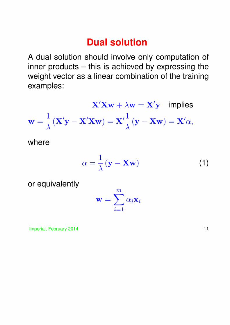
Dual solutionA dual solution should involve only computation ofinner products – this is achieved by expressing theweight vector as a linear combination of the trainingexamples:
X′Xw + λw = X′y implies
w =1
λ(X′y −X′Xw) = X′1
λ(y −Xw) = X′α,
where
α =1
λ(y −Xw) (1)
or equivalently
w =
m∑i=1
αixi
Imperial, February 2014 11

Dual solution
Substituting w = X′α into equation (1) we obtain:
λα = y −XX′α
implying(XX′ + λIm)α = y
This gives the dual solution:
α = (XX′ + λIm)−1
y
and regression function
g(x) = x′w = x′X′α =
m∑i=1
αi⟨x,xi⟩
Imperial, February 2014 12

Key ingredients of dual solution
Step 1: Compute
α = (K+ λIm)−1
y
where K = XX′ that is Kij = ⟨xi,xj⟩
Step 2: Evaluate on new point x by
g(x) =
m∑i=1
αi⟨x,xi⟩
Important observation: Both steps only involveinner products
Imperial, February 2014 13
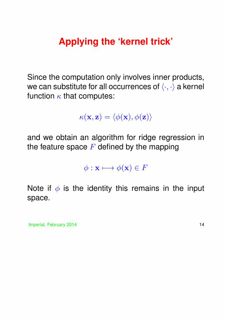
Applying the ‘kernel trick’
Since the computation only involves inner products,we can substitute for all occurrences of ⟨·, ·⟩ a kernelfunction κ that computes:
κ(x, z) = ⟨ϕ(x), ϕ(z)⟩
and we obtain an algorithm for ridge regression inthe feature space F defined by the mapping
ϕ : x 7−→ ϕ(x) ∈ F
Note if ϕ is the identity this remains in the inputspace.
Imperial, February 2014 14

A simple kernel exampleThe simplest non-trivial kernel function is thequadratic kernel:
κ(x, z) = ⟨x, z⟩2
involving just one extra operation. But surprisinglythis kernel function now corresponds to a complexfeature mapping:
κ(x, z) = (x′z)2 = z′(xx′)z
= ⟨vec(zz′), vec(xx′)⟩
where vec(A) stacks the columns of the matrix Aon top of each other. Hence, κ corresponds to thefeature mapping
ϕ : x 7−→ vec(xx′)
Imperial, February 2014 15

Implications of the kernel trick
• Consider for example computing a regressionfunction over 1000 images represented by pixelvectors – say 32× 32 = 1024.
• By using the quadratic kernel we implement theregression function in a 1, 000, 000 dimensionalspace
• but actually using less computation for thelearning phase than we did in the original space.
Imperial, February 2014 16

Implications of kernel algorithms
• Can perform linear regression in very high-dimensional (even infinite dimensional) spacesefficiently.
• This is equivalent to performing non-linearregression in the original input space: forexample quadratic kernel leads to solution of theform
g(x) =m∑i=1
αi⟨xi,x⟩2
that is a quadratic polynomial function of thecomponents of the input vector x.
• Using these high-dimensional spaces mustsurely come with a health warning, what aboutthe curse of dimensionality?
Imperial, February 2014 17

Part 2
• Simple classification algorithm
• Principal components analysis.
• Kernel canonical correlation analysis.
Imperial, February 2014 18
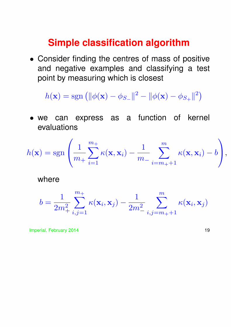
Simple classification algorithm
• Consider finding the centres of mass of positiveand negative examples and classifying a testpoint by measuring which is closest
h(x) = sgn(∥ϕ(x)− ϕS−∥
2 − ∥ϕ(x)− ϕS+∥2)
• we can express as a function of kernelevaluations
h(x) = sgn
1
m+
m+∑i=1
κ(x,xi)−1
m−
m∑i=m++1
κ(x,xi)− b
,
where
b =1
2m2+
m+∑i,j=1
κ(xi,xj)−1
2m2−
m∑i,j=m++1
κ(xi,xj)
Imperial, February 2014 19

Simple classification algorithm
• equivalent to dividing the space with a hyperplaneperpendicular to the line half way between thetwo centres with vector given by
w =1
m+
m+∑i=1
ϕ(xi)−1
m−
m∑i=m++1
ϕ(xi)
• Function is the difference in likelihood of theParzen window density estimators for positiveand negative examples
• We will see some examples of the performanceof this algorithm in a moment.
Imperial, February 2014 20
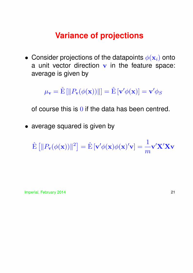
Variance of projections
• Consider projections of the datapoints ϕ(xi) ontoa unit vector direction v in the feature space:average is given by
µv = E [∥Pv(ϕ(x))∥] = E [v′ϕ(x)] = v′ϕS
of course this is 0 if the data has been centred.
• average squared is given by
E[∥Pv(ϕ(x))∥2
]= E [v′ϕ(x)ϕ(x)′v] =
1
mv′X′Xv
Imperial, February 2014 21
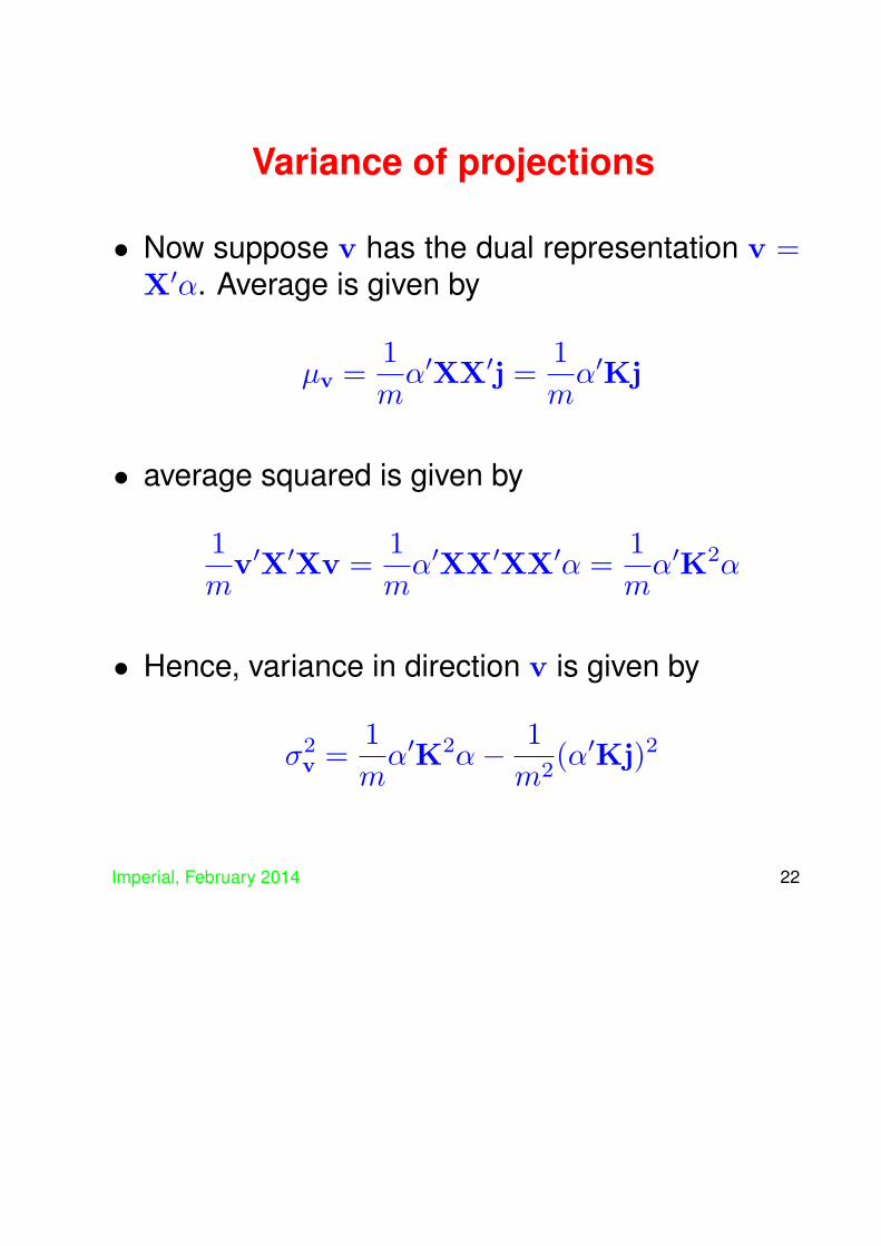
Variance of projections
• Now suppose v has the dual representation v =X′α. Average is given by
µv =1
mα′XX′j =
1
mα′Kj
• average squared is given by
1
mv′X′Xv =
1
mα′XX′XX′α =
1
mα′K2α
• Hence, variance in direction v is given by
σ2v =
1
mα′K2α− 1
m2(α′Kj)2
Imperial, February 2014 22

Fisher discriminant
• The Fisher discriminant is a thresholded linearclassifier:
f(x) = sgn(⟨w, ϕ(x)⟩+ b
where w is chosen to maximise the quotient:
J(w) =(µ+
w − µ−w)
2
(σ+w)2 + (σ−
w)2
• As with Ridge regression it makes sense toregularise if we are working in high-dimensionalkernel spaces, so maximise
J(w) =(µ+
w − µ−w)
2
(σ+w)2 + (σ−
w)2 + λ∥w∥2
Imperial, February 2014 23
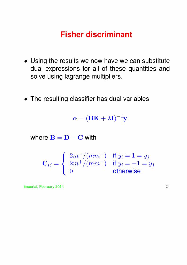
Fisher discriminant
• Using the results we now have we can substitutedual expressions for all of these quantities andsolve using lagrange multipliers.
• The resulting classifier has dual variables
α = (BK+ λI)−1y
where B = D−C with
Cij =
2m−/(mm+) if yi = 1 = yj2m+/(mm−) if yi = −1 = yj0 otherwise
Imperial, February 2014 24

and
D =
2m−/m if i = j and yi = 12m+/m if i = j and yi = −10 otherwise
and b = 0.5αKt with
ti =
1/m+ if yi = 11/m− if yi = −10 otherwise
giving a decision function
f(x) = sgn
(m∑i=1
αiκ(xi,x)− b
)
Imperial, February 2014 25
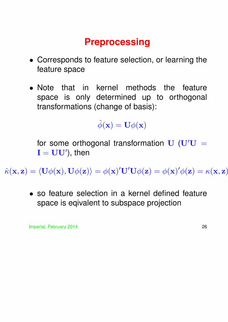
Preprocessing
• Corresponds to feature selection, or learning thefeature space
• Note that in kernel methods the featurespace is only determined up to orthogonaltransformations (change of basis):
ϕ(x) = Uϕ(x)
for some orthogonal transformation U (U′U =I = UU′), then
κ(x, z) = ⟨Uϕ(x),Uϕ(z)⟩ = ϕ(x)′U′Uϕ(z) = ϕ(x)′ϕ(z) = κ(x, z)
• so feature selection in a kernel defined featurespace is eqivalent to subspace projection
Imperial, February 2014 26
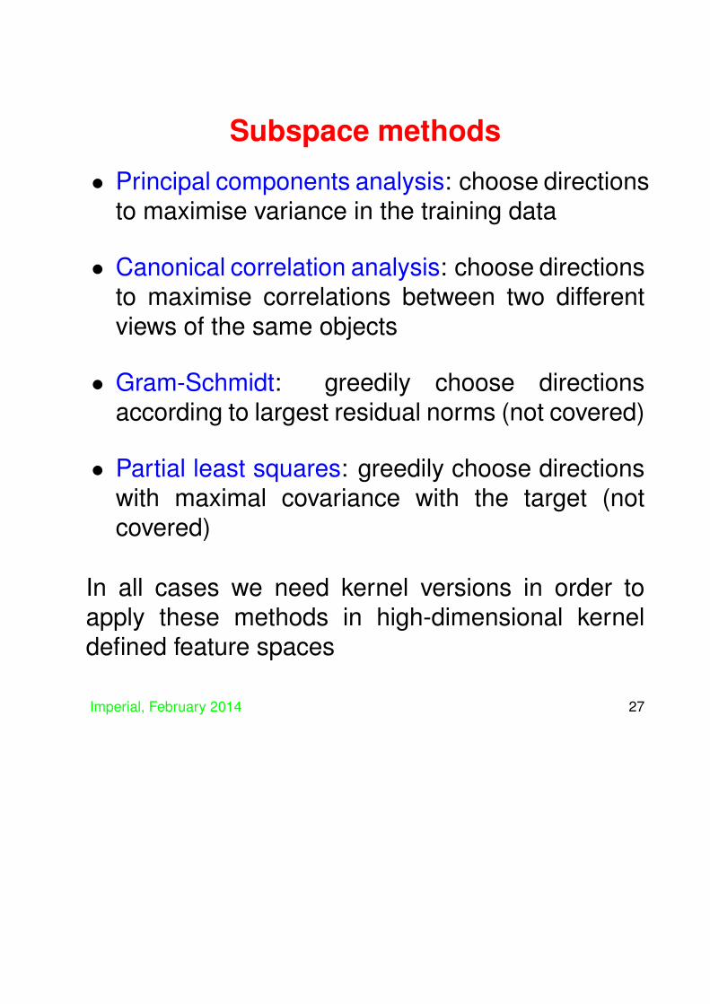
Subspace methods
• Principal components analysis: choose directionsto maximise variance in the training data
• Canonical correlation analysis: choose directionsto maximise correlations between two differentviews of the same objects
• Gram-Schmidt: greedily choose directionsaccording to largest residual norms (not covered)
• Partial least squares: greedily choose directionswith maximal covariance with the target (notcovered)
In all cases we need kernel versions in order toapply these methods in high-dimensional kerneldefined feature spaces
Imperial, February 2014 27

Principal Components Analysis
• PCA is a subspace method – that is it involvesprojecting the data into a lower dimensionalspace.
• Subspace is chosen to ensure maximal varianceof the projections:
w = argmaxw:∥w∥=1w′X′Xw
• This is equivalent to maximising the Raleighquotient:
w′X′Xw
w′w
Imperial, February 2014 28

Principal Components Analysis
• We can optimise using Lagrange multipliers inorder to remove the contraints:
L(w, λ) = w′X′Xw − λw′w
taking derivatives wrt w and setting equal to 0gives:
X′Xw = λw
implying w is an eigenvector of X′X.
• Note that
λ = w′X′Xw =
m∑i=1
⟨w,xi⟩2
Imperial, February 2014 29

Principal Components Analysis
• So principal components analysis performs aneigenvalue decomposition of X′X and projectsinto the space spanned by the first k eigenvectors
• Captures a total of
k∑i=1
λi
of the overall variance:
m∑i=1
∥xi∥2 =n∑
i=1
λi = tr(K)
Imperial, February 2014 30
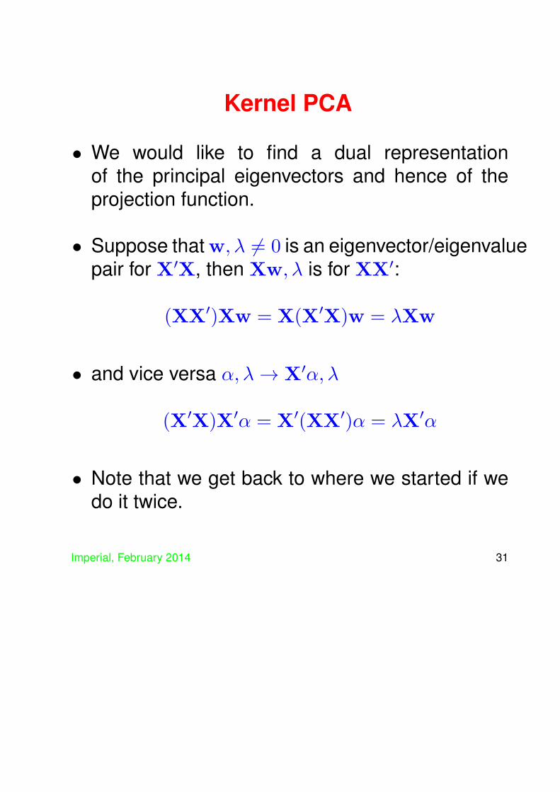
Kernel PCA
• We would like to find a dual representationof the principal eigenvectors and hence of theprojection function.
• Suppose that w, λ = 0 is an eigenvector/eigenvaluepair for X′X, then Xw, λ is for XX′:
(XX′)Xw = X(X′X)w = λXw
• and vice versa α, λ → X′α, λ
(X′X)X′α = X′(XX′)α = λX′α
• Note that we get back to where we started if wedo it twice.
Imperial, February 2014 31

Kernel PCA
• Hence, 1-1 correspondence between eigenvectorscorresponding to non-zero eigenvalues, but notethat if ∥α∥ = 1
∥X′α∥2 = α′XX′α = α′Kα = λ
so if αi, λi, i = 1, . . . , k are first k eigenvectors/valuesof K
1√λi
αi
are dual representations of first k eigenvectorsw1, . . . ,wk of X′X with same eigenvalues.
• Computing projections:
⟨wi, ϕ(x)⟩ = 1√λi
⟨X′αi, ϕ(x)⟩ = 1√λi
m∑j=1
αijκ(xi,x)
Imperial, February 2014 32

Part 3
• Statistical analysis of the stability of patterns.
• Rademacher complexity.
• Generalisation of SVMs
• Support Vector Machine Optimisation
Imperial, February 2014 33

Generalisation of a learner
• Assume that we have a learning algorithm A thatchooses a function AF(S) from a function spaceF in response to the training set S.
• From a statistical point of view the quantity ofinterest is the random variable:
ϵ(S,A,F) = E(x,y) [ℓ(AF(S),x, y)] ,
where ℓ is a ‘loss’ function that measures thediscrepancy between AF(S)(x) and y.
Imperial, February 2014 34

Generalisation of a learner
• For example, in the case of classification ℓ is 1if the two disagree and 0 otherwise, while forregression it could be the square of the differencebetween AF(S)(x) and y.
• We refer to the random variable ϵ(S,A,F) as thegeneralisation of the learner.
Imperial, February 2014 35

Example of Generalisation I
• We consider the Breast Cancer dataset from theUCI repository.
• Use the simple Parzen window classifier describedin Part 2: weight vector is
w+ −w−
where w+ is the average of the positive trainingexamples and w− is average of negative trainingexamples. Threshold is set so hyperplanebisects the line joining these two points.
Imperial, February 2014 36

Example of Generalisation II• Given a size m of the training set, by repeatedly
drawing random training sets S we estimate thedistribution of
ϵ(S,A,F) = E(x,y) [ℓ(AF(S),x, y)] ,
by using the test set error as a proxy for the truegeneralisation.
• We plot the histogram and the average of thedistribution for various sizes of training set –initially the whole dataset gives a single value ifwe use training and test as the all the examples,but then we plot for training set sizes:
342, 273, 205, 137, 68, 34, 27, 20, 14, 7.
Imperial, February 2014 37

Example of Generalisation III
• Since the expected classifier is in all cases thesame:
E [AF(S)] = ES
[w+
S −w−S
]= ES
[w+
S
]− ES
[w−
S
]= Ey=+1 [x]− Ey=−1 [x] ,
we do not expect large differences in the averageof the distribution, though the non-linearity ofthe loss function means they won’t be the sameexactly.
Imperial, February 2014 38

Error distribution: full dataset
0 0.1 0.2 0.3 0.4 0.5 0.6 0.7 0.8 0.9 10
10
20
30
40
50
60
70
80
90
100
Imperial, February 2014 39

Error distribution: dataset size: 342
0 0.1 0.2 0.3 0.4 0.5 0.6 0.7 0.8 0.9 10
5
10
15
20
25
30
Imperial, February 2014 40
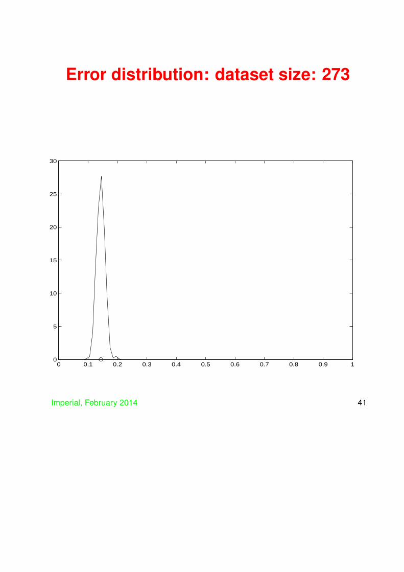
Error distribution: dataset size: 273
0 0.1 0.2 0.3 0.4 0.5 0.6 0.7 0.8 0.9 10
5
10
15
20
25
30
Imperial, February 2014 41

Error distribution: dataset size: 205
0 0.1 0.2 0.3 0.4 0.5 0.6 0.7 0.8 0.9 10
5
10
15
20
25
30
35
Imperial, February 2014 42

Error distribution: dataset size: 137
0 0.1 0.2 0.3 0.4 0.5 0.6 0.7 0.8 0.9 10
5
10
15
20
25
30
Imperial, February 2014 43
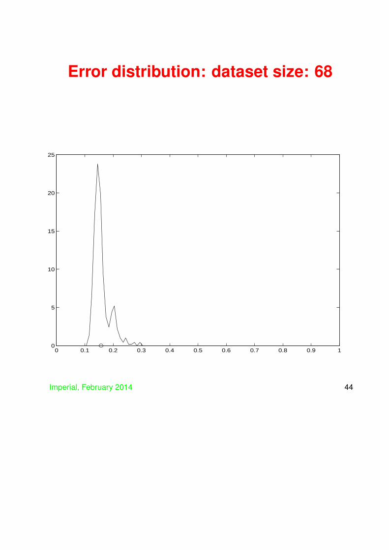
Error distribution: dataset size: 68
0 0.1 0.2 0.3 0.4 0.5 0.6 0.7 0.8 0.9 10
5
10
15
20
25
Imperial, February 2014 44

Error distribution: dataset size: 34
0 0.1 0.2 0.3 0.4 0.5 0.6 0.7 0.8 0.9 10
2
4
6
8
10
12
14
16
18
20
Imperial, February 2014 45
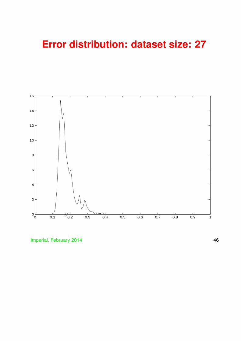
Error distribution: dataset size: 27
0 0.1 0.2 0.3 0.4 0.5 0.6 0.7 0.8 0.9 10
2
4
6
8
10
12
14
16
Imperial, February 2014 46

Error distribution: dataset size: 20
0 0.1 0.2 0.3 0.4 0.5 0.6 0.7 0.8 0.9 10
2
4
6
8
10
12
Imperial, February 2014 47

Error distribution: dataset size: 14
0 0.1 0.2 0.3 0.4 0.5 0.6 0.7 0.8 0.9 10
2
4
6
8
10
12
Imperial, February 2014 48

Error distribution: dataset size: 7
0 0.1 0.2 0.3 0.4 0.5 0.6 0.7 0.8 0.9 10
1
2
3
4
5
6
Imperial, February 2014 49
Observations
• Things can get bad if number of trainingexamples small compared to dimension (in thiscase input dimension is 9)
• Mean can be bad predictor of true generalisationi.e. things can look okay in expectation, but stillgo badly wrong
• Key ingredient of learning keep flexibility highwhile still ensuring good generalisation
Imperial, February 2014 50

Controlling generalisation
• The critical method of controlling generalisationfor classification is to force a large margin on thetraining data
• Equivalent to minimising the norm while keepingthe separation fixed (at say ±1)
• Support Vector Machines implement this strategy
Imperial, February 2014 51

Controlling generalisation
• Now consider using an SVM on the same dataand compare the distribution of generalisations
• SVM distribution in red
Imperial, February 2014 52

Error distribution: dataset size: 205
0 0.2 0.4 0.6 0.8 10
5
10
15
20
25
30
35
Imperial, February 2014 53
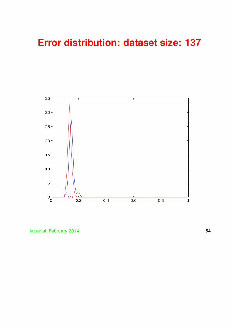
Error distribution: dataset size: 137
0 0.2 0.4 0.6 0.8 10
5
10
15
20
25
30
35
Imperial, February 2014 54

Error distribution: dataset size: 68
0 0.2 0.4 0.6 0.8 10
5
10
15
20
25
30
Imperial, February 2014 55
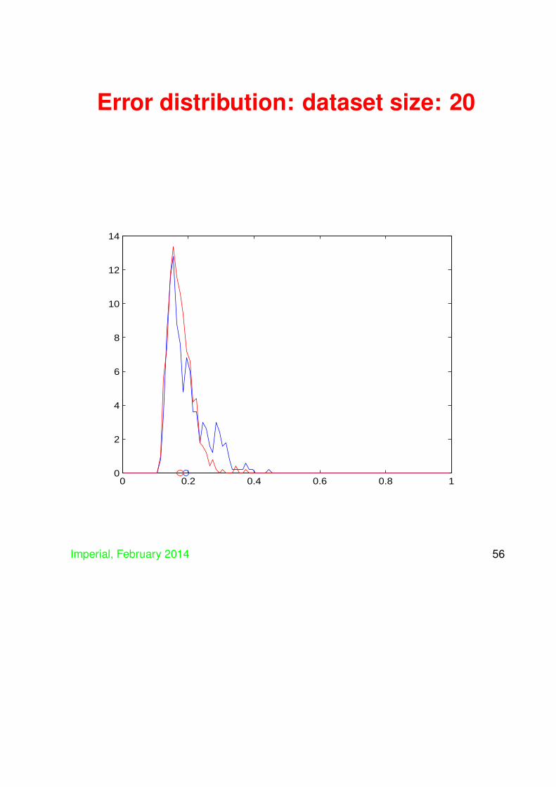
Error distribution: dataset size: 20
0 0.2 0.4 0.6 0.8 10
2
4
6
8
10
12
14
Imperial, February 2014 56

Error distribution: dataset size: 14
0 0.2 0.4 0.6 0.8 10
5
10
15
Imperial, February 2014 57
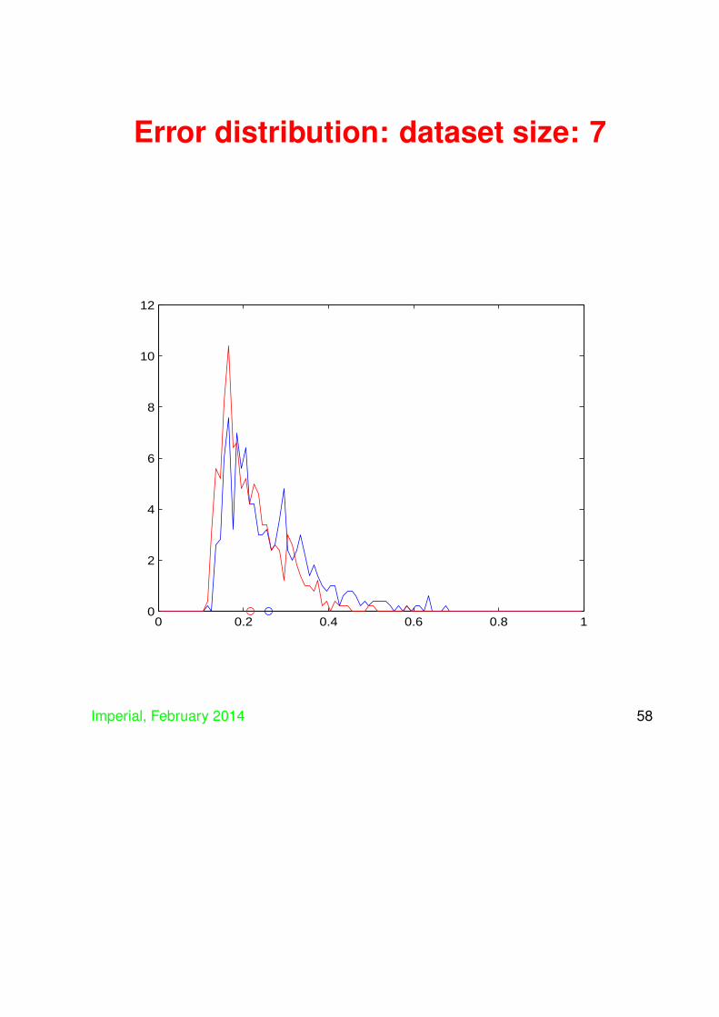
Error distribution: dataset size: 7
0 0.2 0.4 0.6 0.8 10
2
4
6
8
10
12
Imperial, February 2014 58

Expected versus confident bounds
• For a finite sample the generalisation ϵ(S,A,F)has a distribution depending on the algorithm,function class and sample size m.
• Traditional statistics as indicated above hasconcentrated on the mean of this distribution –but this quantity can be misleading, eg for lowfold cross-validation.
Imperial, February 2014 59

Expected versus confident boundscont.
• Statistical learning theory has preferred toanalyse the tail of the distribution, finding a boundwhich holds with high probability.
• This looks like a statistical test – significant at a1% confidence means that the chances of theconclusion not being true are less than 1% overrandom samples of that size.
• This is also the source of the acronym PAC:probably approximately correct, the ‘confidence’parameter δ is the probability that we have beenmisled by the training set.
Imperial, February 2014 60

Concentration inequalities
• Statistical Learning is concerned with thereliability or stability of inferences made from arandom sample.
• Random variables with this property have beena subject of ongoing interest to probabilists andstatisticians.
Imperial, February 2014 61

Concentration inequalities cont.
• As an example consider the mean of a sample ofm 1-dimensional random variables X1, . . . , Xm:
Sm =1
m
m∑i=1
Xi.
• Hoeffding’s inequality states that if Xi ∈ [ai, bi]
P{|Sm − E[Sm]| ≥ ϵ} ≤ 2 exp
(− 2m2ϵ2∑m
i=1(bi − ai)2
)Note how the probability falls off exponentiallywith the distance from the mean and with thenumber of variables.
Imperial, February 2014 62

Concentration for SLT
• We are now going to look at deriving SLT resultsfrom concentration inequalities.
• Perhaps the best known form is due toMcDiarmid (although he was actually representingpreviously derived results):
Imperial, February 2014 63

McDiarmid’s inequalityTheorem 1. Let X1, . . . , Xn be independent randomvariables taking values in a set A, and assume thatf : An → R satisfies
supx1,...,xn,xi∈A
|f(x1, . . . , xn)− f(x1, . . . , xi, xi+1, . . . , xn)| ≤ ci,
for 1 ≤ i ≤ n. Then for all ϵ > 0,
P {f (X1, . . . , Xn)− Ef (X1, . . . , Xn) ≥ ϵ} ≤ exp
(−2ϵ2∑ni=1 c
2i
)
• Hoeffding is a special case when f(x1, . . . , xn) =Sn
Imperial, February 2014 64

Using McDiarmid
• By setting the right hand side equal to δ, we canalways invert McDiarmid to get a high confidencebound: with probability at least 1− δ
f (X1, . . . , Xn) < Ef (X1, . . . , Xn) +
√∑ni=1 c
2i
2log
1
δ
• If ci = c/n for each i this reduces to
f (X1, . . . , Xn) < Ef (X1, . . . , Xn) +
√c2
2nlog
1
δ
Imperial, February 2014 65

Rademacher complexity
• Rademacher complexity is a new way ofmeasuring the complexity of a function class. Itarises naturally if we rerun the proof using thedouble sample trick and symmetrisation but lookat what is actually needed to continue the proof:
Imperial, February 2014 66

Rademacher proof beginningsFor a fixed f ∈ F we have
E [f(z)] ≤ E [f(z)] + suph∈F
(E[h]− E[h]
).
where F is a class of functions mapping from Z to[0, 1] and E denotes the sample average.
We must bound the size of the second term. Firstapply McDiarmid’s inequality to obtain (ci = 1/m forall i) with probability at least 1− δ:
suph∈F
(E[h]− E[h]
)≤ ES
[suph∈F
(E[h]− E[h]
)]+
√ln(1/δ)
2m.
Imperial, February 2014 67
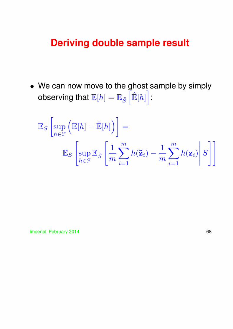
Deriving double sample result
• We can now move to the ghost sample by simplyobserving that E[h] = ES
[E[h]
]:
ES
[suph∈F
(E[h]− E[h]
)]=
ES
[suph∈F
ES
[1
m
m∑i=1
h(zi)−1
m
m∑i=1
h(zi)
∣∣∣∣∣S]]
Imperial, February 2014 68

Deriving double sample result cont.
Since the sup of an expectation is less than orequal to the expectation of the sup (we can makethe choice to optimise for each S) we have
ES
[suph∈F
(E[h]− E[h]
)]≤
ESES
[suph∈F
1
m
m∑i=1
(h(zi)− h(zi))
]
Imperial, February 2014 69
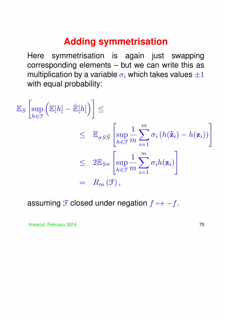
Adding symmetrisationHere symmetrisation is again just swappingcorresponding elements – but we can write this asmultiplication by a variable σi which takes values ±1with equal probability:
ES
[suph∈F
(E[h]− E[h]
)]≤
≤ EσSS
[suph∈F
1
m
m∑i=1
σi (h(zi)− h(zi))
]
≤ 2ESσ
[suph∈F
1
m
m∑i=1
σih(zi)
]= Rm (F) ,
assuming F closed under negation f 7→ −f .
Imperial, February 2014 70

Rademacher complexity
The Rademacher complexity provides a way ofmeasuring the complexity of a function class F bytesting how well on average it can align with randomnoise:
Rm(F) = ESσ
[supf∈F
2
m
m∑i=1
σif (zi)
].
is known as the Rademacher complexity of thefunction class F.
Imperial, February 2014 71

Main Rademacher theorem
The main theorem of Rademacher complexity: withprobability at least 1 − δ over random samples S ofsize m, every f ∈ F satisfies
E [f(z)] ≤ E [f(z)] +Rm(F) +
√ln(1/δ)
2m
• Note that Rademacher complexity gives theexpected value of the maximal correlation withrandom noise – a very natural measure ofcapacity.
• Note that the Rademacher complexity is distributiondependent since it involves an expectation overthe choice of sample – this might seem hard tocompute.
Imperial, February 2014 72
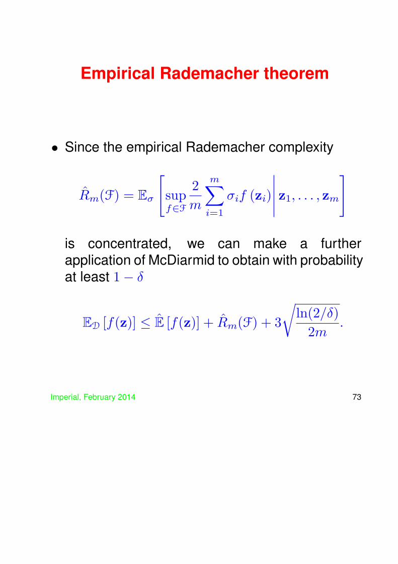
Empirical Rademacher theorem
• Since the empirical Rademacher complexity
Rm(F) = Eσ
[supf∈F
2
m
m∑i=1
σif (zi)
∣∣∣∣∣ z1, . . . , zm]
is concentrated, we can make a furtherapplication of McDiarmid to obtain with probabilityat least 1− δ
ED [f(z)] ≤ E [f(z)] + Rm(F) + 3
√ln(2/δ)
2m.
Imperial, February 2014 73

Application to large marginclassification
• Rademacher complexity comes into its own forBoosting and SVMs.
Imperial, February 2014 74

Application to Boosting
• We can view Boosting as seeking a function fromthe class (H is the set of weak learners){∑
h∈H
ahh(x) : ah ≥ 0,∑h∈H
ah ≤ B
}= convB(H)
by minimising some function of the margindistribution (assume H closed under negation).
• Adaboost corresponds to optimising an exponentialfunction of the margin over this set of functions.
• We will see how to include the margin in theanalysis later, but concentrate on computing theRademacher complexity for now.
Imperial, February 2014 75

Rademacher complexity for SVMs
• The Rademacher complexity of a class of linearfunctions with bounded 2-norm:{x →
m∑i=1
αiκ(xi,x):α′Kα ≤ B2
}⊆
⊆ {x → ⟨w, ϕ (x)⟩ : ∥w∥ ≤ B}= FB,
where we assume a kernel defined featurespace with
⟨ϕ(x), ϕ(z)⟩ = κ(x, z).
Imperial, February 2014 76

Rademacher complexity of FBThe following derivation gives the result
Rm(FB) = Eσ
[supf∈FB
∣∣∣∣∣ 2mm∑i=1
σif (xi)
∣∣∣∣∣]
= Eσ
[sup
∥w∥≤B
∣∣∣∣∣⟨w,
2
m
m∑i=1
σiϕ (xi)
⟩∣∣∣∣∣]
≤ 2B
mEσ
[∥∥∥∥∥m∑i=1
σiϕ(xi)
∥∥∥∥∥]
=2B
mEσ
⟨ m∑
i=1
σiϕ(xi),
m∑j=1
σjϕ(xj)
⟩1/2
≤ 2B
m
Eσ
m∑i,j=1
σiσjκ(xi,xj)
1/2
=2B
m
√√√√ m∑i=1
κ(xi,xi)
Imperial, February 2014 77

Imperial, February 2014 78
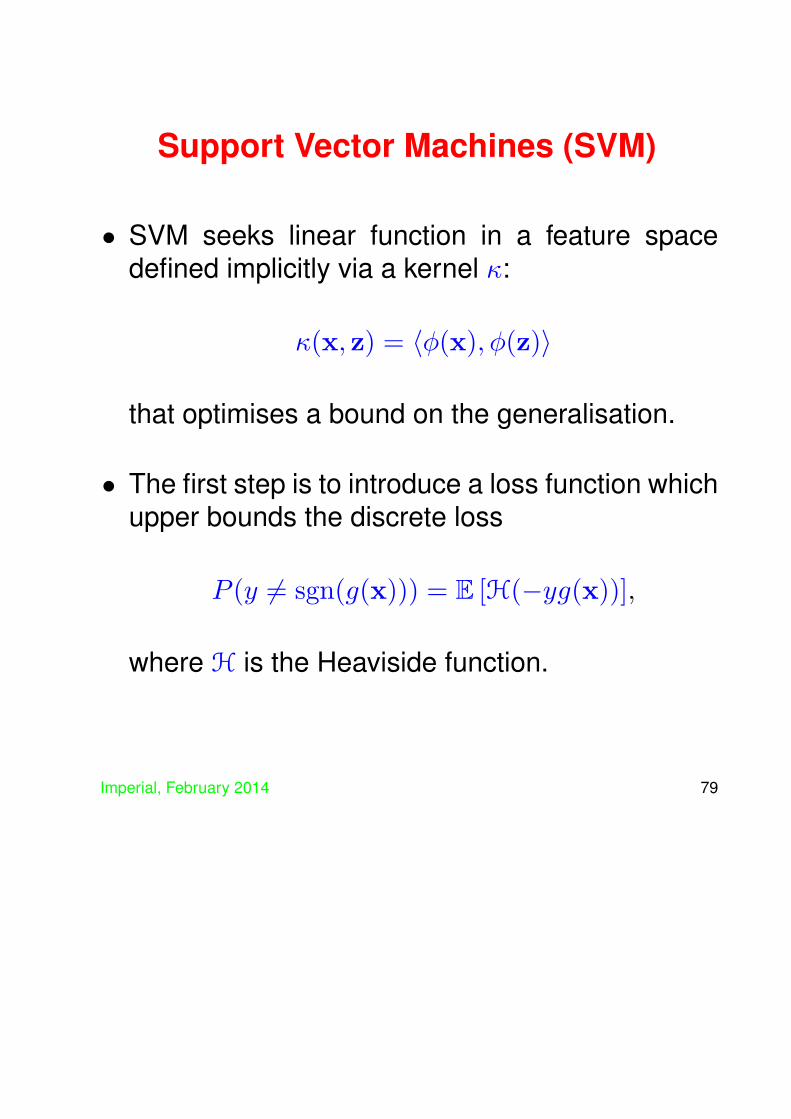
Support Vector Machines (SVM)
• SVM seeks linear function in a feature spacedefined implicitly via a kernel κ:
κ(x, z) = ⟨ϕ(x), ϕ(z)⟩
that optimises a bound on the generalisation.
• The first step is to introduce a loss function whichupper bounds the discrete loss
P (y = sgn(g(x))) = E [H(−yg(x))],
where H is the Heaviside function.
Imperial, February 2014 79

Margins in SVMs
• Critical to the bound will be the margin of theclassifier
γ(x, y) = yg(x) = y(⟨w, ϕ(x)⟩+ b) :
positive if correctly classified, and measuresdistance from the separating hyperplane whenthe weight vector is normalised.
• The margin of a linear function g is
γ(g) = mini
γ(xi, yi)
though this is frequently increased to allow some‘margin errors’.
Imperial, February 2014 80

Margins in SVMs
Imperial, February 2014 81

Applying the Rademacher theorem
• Consider the loss function A : R → [0, 1], givenby
A(a) =
1, if a > 0;1 + a/γ, if −γ ≤ a ≤ 0;0, otherwise.
• By the Rademacher Theorem and since the lossfunction A dominates H, we have that
E [H(−yg(x))] ≤ E [A(−yg(x))]
≤ E [A(−yg(x))] +
Rm(A ◦ F) + 3
√ln(2/δ)
2m.
Imperial, February 2014 82

Imperial, February 2014 83
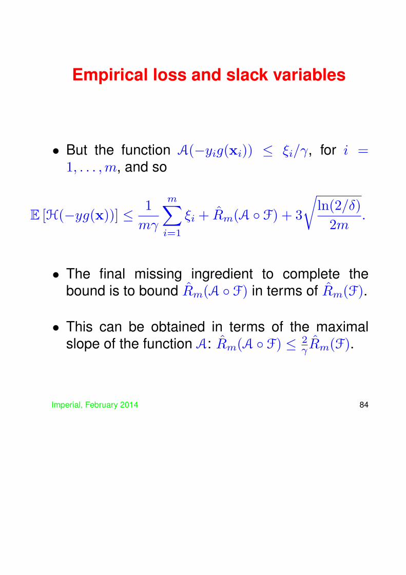
Empirical loss and slack variables
• But the function A(−yig(xi)) ≤ ξi/γ, for i =1, . . . ,m, and so
E [H(−yg(x))] ≤ 1
mγ
m∑i=1
ξi + Rm(A ◦ F) + 3
√ln(2/δ)
2m.
• The final missing ingredient to complete thebound is to bound Rm(A ◦ F) in terms of Rm(F).
• This can be obtained in terms of the maximalslope of the function A: Rm(A ◦ F) ≤ 2
γRm(F).
Imperial, February 2014 84

Final SVM bound
• Assembling the result we obtain:
P (y = sgn(g(x))) = E [H(−yg(x))]
≤ 1
mγ
m∑i=1
ξi +4
mγ
√√√√ m∑i=1
κ(xi,xi) + 3
√ln(2/δ)
2m
• Note that for the Gaussian kernel this reduces to
P (y = sgn(g(x))) ≤ 1
mγ
m∑i=1
ξi +4√mγ
+ 3
√ln(2/δ)
2m
Imperial, February 2014 85

Using a kernel
• Can consider much higher dimensional spacesusing the kernel trick
• Can even work in infinite dimensional spaces, egusing the Gaussian kernel:
κ(x, z) = exp
(−∥x− z∥2
2σ2
)
Imperial, February 2014 86

Error distribution: dataset size: 342
0 0.2 0.4 0.6 0.8 10
5
10
15
20
25
30
35
40
Imperial, February 2014 87
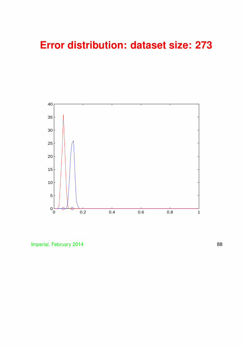
Error distribution: dataset size: 273
0 0.2 0.4 0.6 0.8 10
5
10
15
20
25
30
35
40
Imperial, February 2014 88
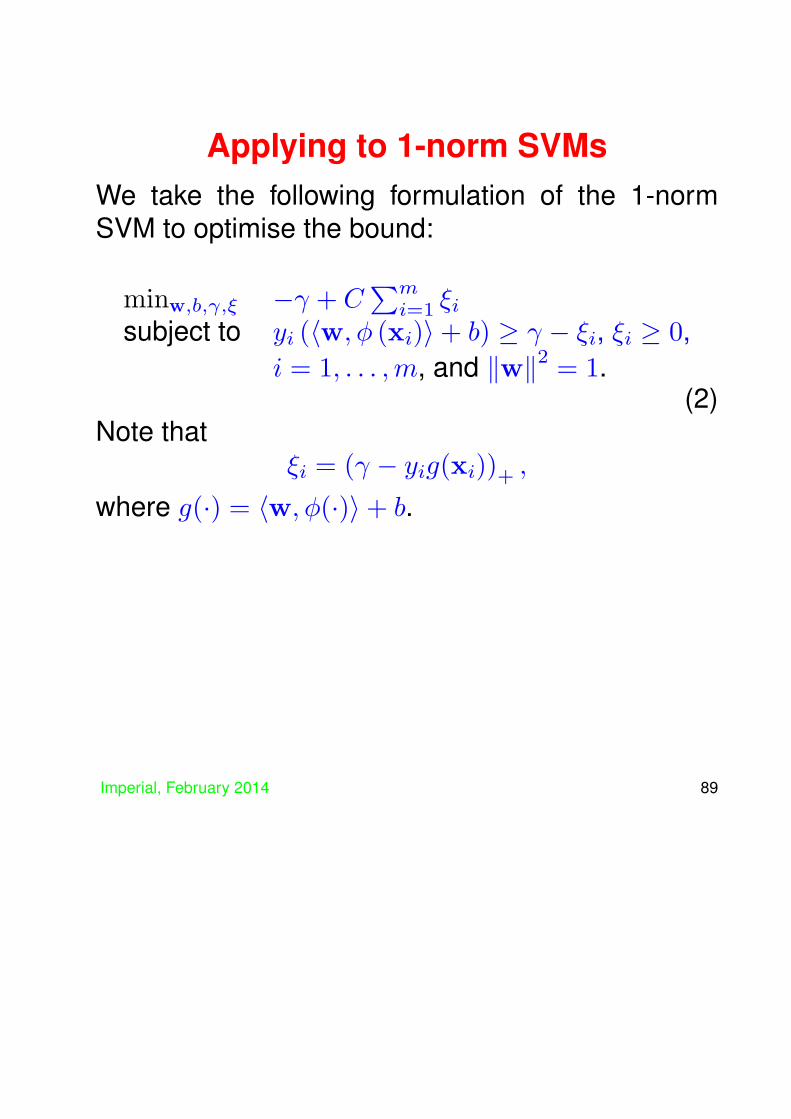
Applying to 1-norm SVMsWe take the following formulation of the 1-normSVM to optimise the bound:
minw,b,γ,ξ −γ + C∑m
i=1 ξisubject to yi (⟨w, ϕ (xi)⟩+ b) ≥ γ − ξi, ξi ≥ 0,
i = 1, . . . ,m, and ∥w∥2 = 1.(2)
Note thatξi = (γ − yig(xi))+ ,
where g(·) = ⟨w, ϕ(·)⟩+ b.
Imperial, February 2014 89
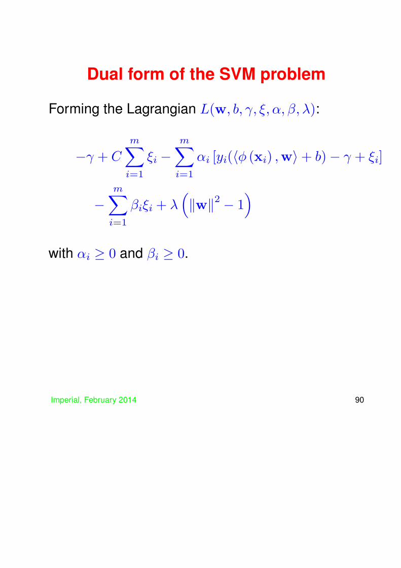
Dual form of the SVM problem
Forming the Lagrangian L(w, b, γ, ξ, α, β, λ):
−γ + C
m∑i=1
ξi −m∑i=1
αi [yi(⟨ϕ (xi) ,w⟩+ b)− γ + ξi]
−m∑i=1
βiξi + λ(∥w∥2 − 1
)with αi ≥ 0 and βi ≥ 0.
Imperial, February 2014 90

Dual form of the SVM problem
Taking derivatives gives:
∂L(w, b, γ, ξ, α, β, λ)
∂w= 2λw −
m∑i=1
yiαiϕ (xi) = 0,
∂L(w, b, γ, ξ, α, β, λ)
∂ξi= C−αi−βi = 0,
∂L(w, b, γ, ξ, α, β, λ)
∂b=
m∑i=1
yiαi = 0,
∂L(w, b, γ, ξ, α, β, λ)
∂γ= 1−
m∑i=1
αi = 0.
Imperial, February 2014 91

Dual form of the SVM problem
L(α, λ) = − 1
4λ
m∑i,j=1
yiyjαiαjκ (xi,xj)− λ,
which, again optimising with respect to λ, gives
λ∗ =1
2
m∑i,j=1
yiyjαiαjκ (xi,xj)
1/2
Imperial, February 2014 92

Dual form of the SVM problem
equivalent to maximising
L(α) = −m∑
i,j=1
αiαjyiyjκ (xi,xj) ,
subject to the constraints
0 ≤ αi ≤ C,
m∑i=1
αi = 1
m∑i=1
yiαi = 0
to give solution
α∗i , i = 1, . . . ,m
Imperial, February 2014 93

Dual form of the SVM problemThis is a convex quadratic programme: minimisinga convex quadratic objective subject to linearconstraints: convex if Hessian G is positive semi-definite:
Gij = yiyjκ (xi,xj)
Matrix psd iff u′Gu ≥ 0 for all u:
u′Gu =
m∑i,j=1
uiujyiyj⟨ϕ(xi), ϕ(xj)⟩
=
⟨m∑i=1
uiyiϕ(xi),
m∑j=1
ujyjϕ(xj)
⟩
=
∥∥∥∥∥m∑i=1
uiyiϕ(xi)
∥∥∥∥∥2
≥ 0
Imperial, February 2014 94
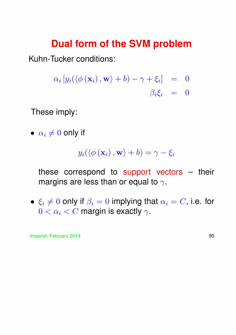
Dual form of the SVM problemKuhn-Tucker conditions:
αi [yi(⟨ϕ (xi) ,w⟩+ b)− γ + ξi] = 0
βiξi = 0
These imply:
• αi = 0 only if
yi(⟨ϕ (xi) ,w⟩+ b) = γ − ξi
these correspond to support vectors – theirmargins are less than or equal to γ.
• ξi = 0 only if βi = 0 implying that αi = C, i.e. for0 < αi < C margin is exactly γ.
Imperial, February 2014 95
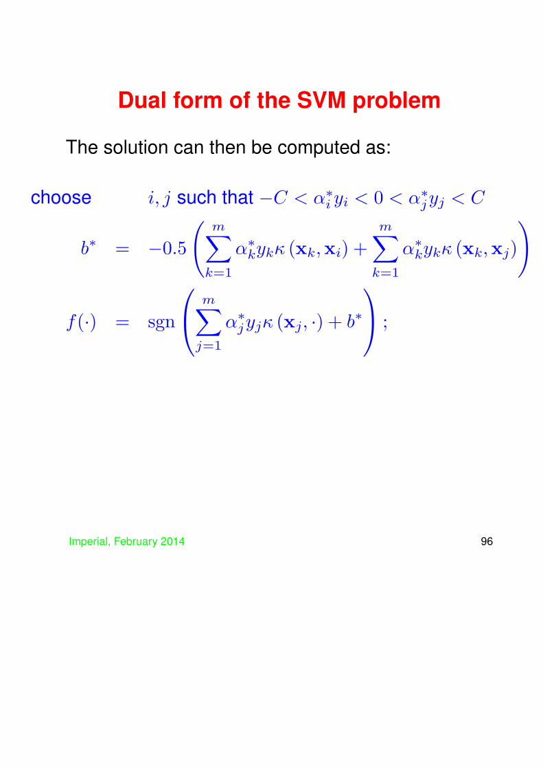
Dual form of the SVM problem
The solution can then be computed as:
choose i, j such that −C < α∗i yi < 0 < α∗
jyj < C
b∗ = −0.5
(m∑
k=1
α∗kykκ (xk,xi) +
m∑k=1
α∗kykκ (xk,xj)
)
f(·) = sgn
m∑j=1
α∗jyjκ (xj, ·) + b∗
;
Imperial, February 2014 96
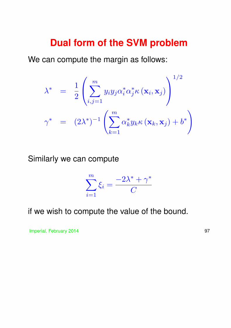
Dual form of the SVM problem
We can compute the margin as follows:
λ∗ =1
2
m∑i,j=1
yiyjα∗iα
∗jκ (xi,xj)
1/2
γ∗ = (2λ∗)−1
(m∑
k=1
α∗kykκ (xk,xj) + b∗
)
Similarly we can compute
m∑i=1
ξi =−2λ∗ + γ∗
C
if we wish to compute the value of the bound.
Imperial, February 2014 97

Dual form of the SVM problem
Decision boundary and γ margin for 1-norm svmwith a gaussian kernel:
Imperial, February 2014 98

Dual form of the SVM problem
• Have introduced a slightly non-standard versionof the SVM but makes ν-SVM very simple todefine.
• Consider expressing C = 1/(νm):
– implies 0 ≤ αi ≤ 1/(νm)– if ξ > 0 then αi = 1/(νm), but
∑mi=1αi = 1 so
at most νm inputs can have this hold.– equally at least νm inputs have αi = 0
• Hence, ν can be seen as the fraction of ‘supportvectors’, a natural measure of the noise in thedata.
Imperial, February 2014 99

Alternative form of the SVM problem
Note more traditional form of the dual SVMoptimisation:
L(α) =
m∑i=1
αi −1
2
m∑i,j=1
αiαjyiyjκ (xi,xj) .
with constraints
0 ≤ αi ≤ C,
m∑i=1
yiαi = 0
Imperial, February 2014 100
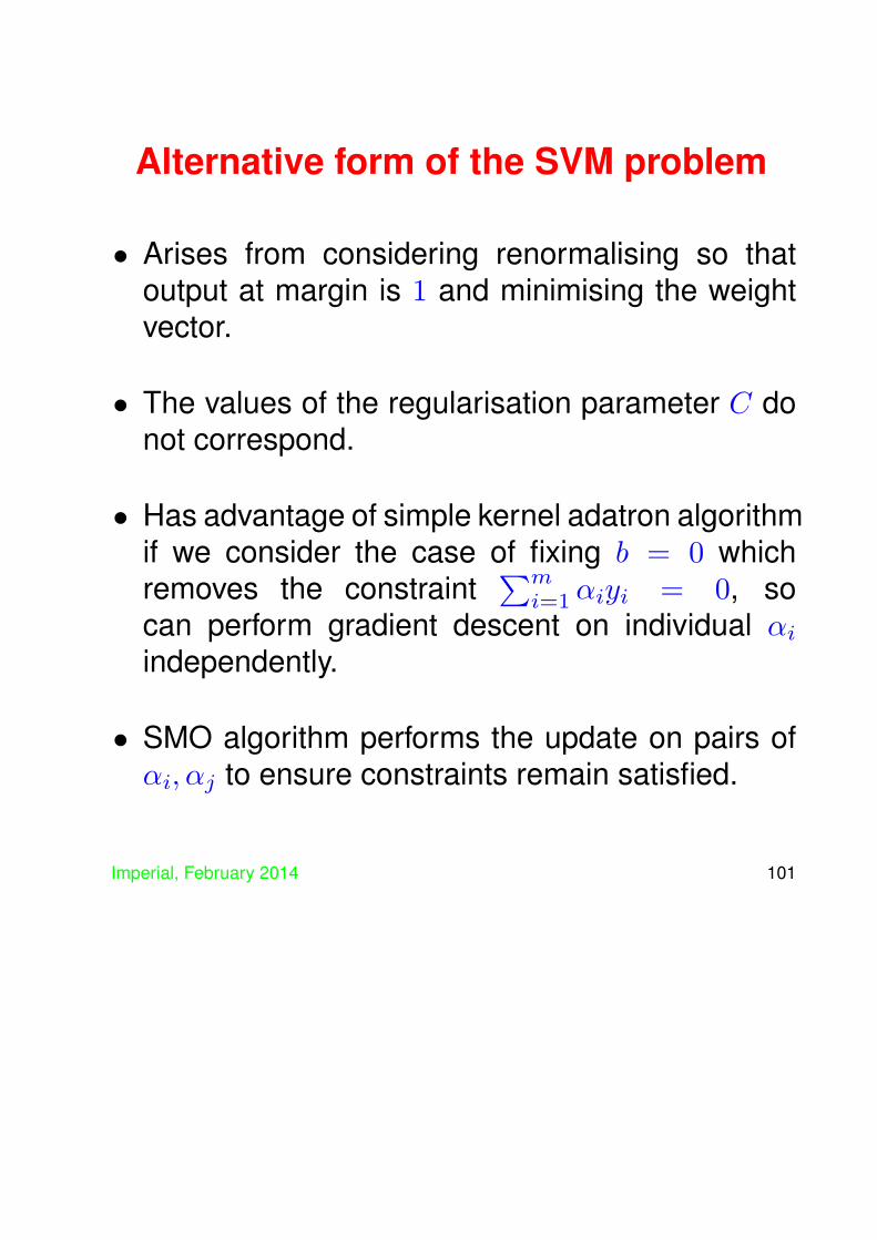
Alternative form of the SVM problem
• Arises from considering renormalising so thatoutput at margin is 1 and minimising the weightvector.
• The values of the regularisation parameter C donot correspond.
• Has advantage of simple kernel adatron algorithmif we consider the case of fixing b = 0 whichremoves the constraint
∑mi=1αiyi = 0, so
can perform gradient descent on individual αi
independently.
• SMO algorithm performs the update on pairs ofαi, αj to ensure constraints remain satisfied.
Imperial, February 2014 101

Part 4
• Kernel design strategies.
• Kernels for text and string kernels.
• Kernels for other structures.
• Kernels from generative models.
Imperial, February 2014 102

Kernel functions• Already seen some properties of kernels:
– symmetric:
κ(x, z) = ⟨ϕ(x), ϕ(z)⟩ = ⟨ϕ(z), ϕ(x)⟩ = κ(z,x)
– kernel matrices psd:
u′Ku =
m∑i,j=1
uiuj⟨ϕ(xi), ϕ(xj)⟩
=
⟨m∑i=1
uiϕ(xi),
m∑j=1
ujϕ(xj)
⟩
=
∥∥∥∥∥m∑i=1
uiϕ(xi)
∥∥∥∥∥2
≥ 0
Imperial, February 2014 103

Kernel functions
• These two properties are all that is required for akernel function to be valid: symmetric and everykernel matrix is psd.
• Note that this is equivalent to all eigenvalues non-negative – recall that eigenvalues of the kernelmatrix measured the sum of the squares of theprojections onto the eigenvector.
• If we have uncountable domains should alsohave continuity, though there are exceptions tothis as well.
Imperial, February 2014 104
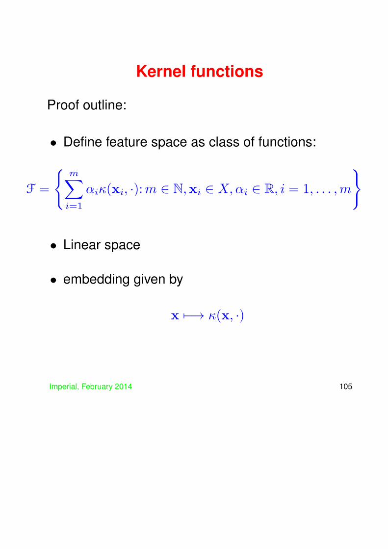
Kernel functions
Proof outline:
• Define feature space as class of functions:
F =
{m∑i=1
αiκ(xi, ·):m ∈ N,xi ∈ X,αi ∈ R, i = 1, . . . ,m
}
• Linear space
• embedding given by
x 7−→ κ(x, ·)
Imperial, February 2014 105

Kernel functions
• inner product between
f(x) =
m∑i=1
αiκ(xi,x) and g(x) =
n∑i=1
βiκ(zi,x)
defined as
⟨f, g⟩ =m∑i=1
n∑j=1
αiβjκ(xi, zj) =m∑i=1
αig(xi) =n∑
j=1
βjf(zj),
• well-defined
• ⟨f, f⟩ ≥ 0 by psd property.
Imperial, February 2014 106

Kernel functions
• so-called reproducing property:
⟨f, ϕ(x)⟩ = ⟨f, κ(x, ·)⟩ = f(x)
• implies that inner product corresponds tofunction evaluation – learning a function correspondsto learning a point being the weight vectorcorresponding to that function:
⟨wf , ϕ(x)⟩ = f(x)
Imperial, February 2014 107

Kernel constructions
For κ1, κ2 valid kernels, ϕ any feature map, B psdmatrix, a ≥ 0 and f any real valued function, thefollowing are valid kernels:
• κ(x, z) = κ1(x, z) + κ2(x, z),
• κ(x, z) = aκ1(x, z),
• κ(x, z) = κ1(x, z)κ2(x, z),
• κ(x, z) = f(x)f(z),
• κ(x, z) = κ1(ϕ(x),ϕ(z)),
• κ(x, z) = x′Bz.
Imperial, February 2014 108

Kernel constructionsFollowing are also valid kernels:
• κ(x, z) =p(κ1(x, z)), for p any polynomial withpositive coefficients.
• κ(x, z) = exp(κ1(x, z)),
• κ(x, z) = exp(−∥x− z∥2 /(2σ2)).
Proof of third: normalise the second kernel:
exp(⟨x, z⟩ /σ2)√exp(∥x∥2 /σ2) exp(∥z∥2 /σ2)
= exp
(⟨x, z⟩σ2
− ⟨x,x⟩2σ2
− ⟨z, z⟩2σ2
)
= exp
(−∥x− z∥2
2σ2
).
Imperial, February 2014 109

Subcomponents kernelFor the kernel ⟨x, z⟩s the features can be indexed bysequences
i = (i1, . . . , in),
n∑j=1
ij = s
whereϕi(x) = xi1
1 xi22 . . . xin
n
A similar kernel can be defined in which all subsetsof features occur:
ϕ : x 7→ (ϕA(x))A⊆{1,...,n}
whereϕA(x) =
∏i∈A
xi
Imperial, February 2014 110
Subcomponents kernel
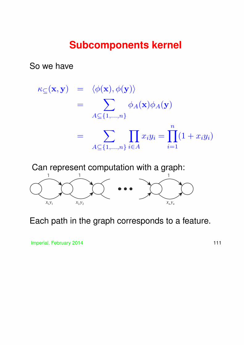
So we have
κ⊆(x,y) = ⟨ϕ(x), ϕ(y)⟩
=∑
A⊆{1,...,n}
ϕA(x)ϕA(y)
=∑
A⊆{1,...,n}
∏i∈A
xiyi =n∏
i=1
(1 + xiyi)
Can represent computation with a graph:1
x y1 1
x y2 2
x yn n
1 1
Each path in the graph corresponds to a feature.
Imperial, February 2014 111

Graph kernels
Can also represent polynomial kernel
κ(x,y) = (⟨x,y⟩+R)d= (x1y1 + x2y2 + · · ·+ xnyn +R)
d
with a graph:R
x y 1 1
x y 2 2
x y n n
R x y
1 1
x y 2 2
x y n n
R x y
1 1
x y 2 2
x y n n
d 1 - d 1 2 3
Imperial, February 2014 112

Graph kernels
The ANOVA kernel is represented by the graph:1
x z1 1
0 0( , ) 1
x z1 1
1
1
0 1( , )
1 1( , ) 1
1
( , )0 2
,( )1 2
( , )2 2
x z2 2 x z2 2
1
x z1 1
( , )1 n( , )1 1n -
( , )2 1n - ( , )2 n
( , )d n- -1 1 ( , )d n-1
( , )d n-1 ( , )d n
( , )0 1n- ( , )0 n
1
x zn n
Imperial, February 2014 113

Graph kernels
Features are all the combinations of exactly ddistinct features, while computation is given byrecursion:
κm0 (x, z) = 1, if m ≥ 0,
κms (x, z) = 0, if m < s,
κms (x, z) = (xmzm)κm−1
s−1 (x, z) + κm−1s (x, z)
While the resulting kernel is given by
κnd(x, z)
in the bottom right corner of the graph.
Imperial, February 2014 114

Graph kernels
• Initialise DP(1) = 1;
• for each node compute
DP(i) =∑j→i
κ(uj→ui) (x, z)DP (j)
• result given at output node s: κ(x, z) = DP(s).
Imperial, February 2014 115

Kernels for text
• The simplest representation for text is the kernelgiven by the feature map known as the vectorspace model
ϕ : d 7→ ϕ(d) = (tf(t1, d), tf(t2, d), . . . , tf(tN , d))′
where t1, t2, . . . , tN are the terms occurring in thecorpus and tf(t, d) measures the frequency ofterm t in document d.
• Usually use the notation D for the document termmatrix (cf. X from previous notation).
Imperial, February 2014 116

Kernels for text
• Kernel matrix is given by
K = DD′
wrt kernel
κ(d1, d2) =
N∑j=1
tf(tj, d1)tf(tj, d2)
• despite high-dimensionality kernel function canbe computed efficiently by using a linked listrepresentation.
Imperial, February 2014 117

Semantics for text
• The standard representation does not take intoaccount the importance or relationship betweenwords.
• Main methods do this by introducing a ‘semantic’mapping S:
κ(d1, d2) = ϕ(d1)′SS′ϕ(d2)
Imperial, February 2014 118

Semantics for text
• Simplest is diagonal matrix giving term weightings(known as inverse document frequency – tfidf):
w(t) = lnm
df(t)
• Hence kernel becomes:
κ(d1, d2) =
N∑j=1
w(tj)2tf(tj, d1)tf(tj, d2)
Imperial, February 2014 119

Semantics for text
• In general would also like to include semanticlinks between terms with off-diagonal elements,eg stemming, query expansion, wordnet.
• More generally can use co-occurrence of wordsin documents:
S = D′
so(SS′)ij =
∑d
tf(i, d)tf(j, d)
Imperial, February 2014 120
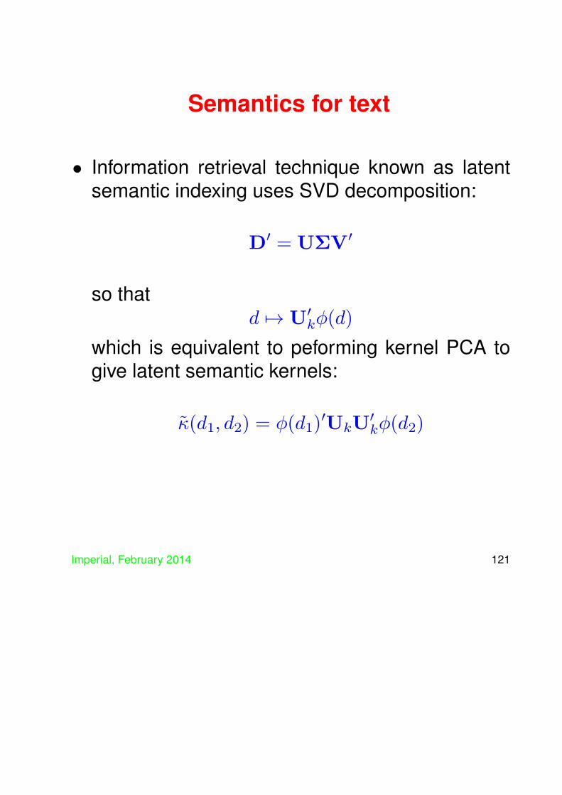
Semantics for text
• Information retrieval technique known as latentsemantic indexing uses SVD decomposition:
D′ = UΣV′
so thatd 7→ U′
kϕ(d)
which is equivalent to peforming kernel PCA togive latent semantic kernels:
κ(d1, d2) = ϕ(d1)′UkU
′kϕ(d2)
Imperial, February 2014 121
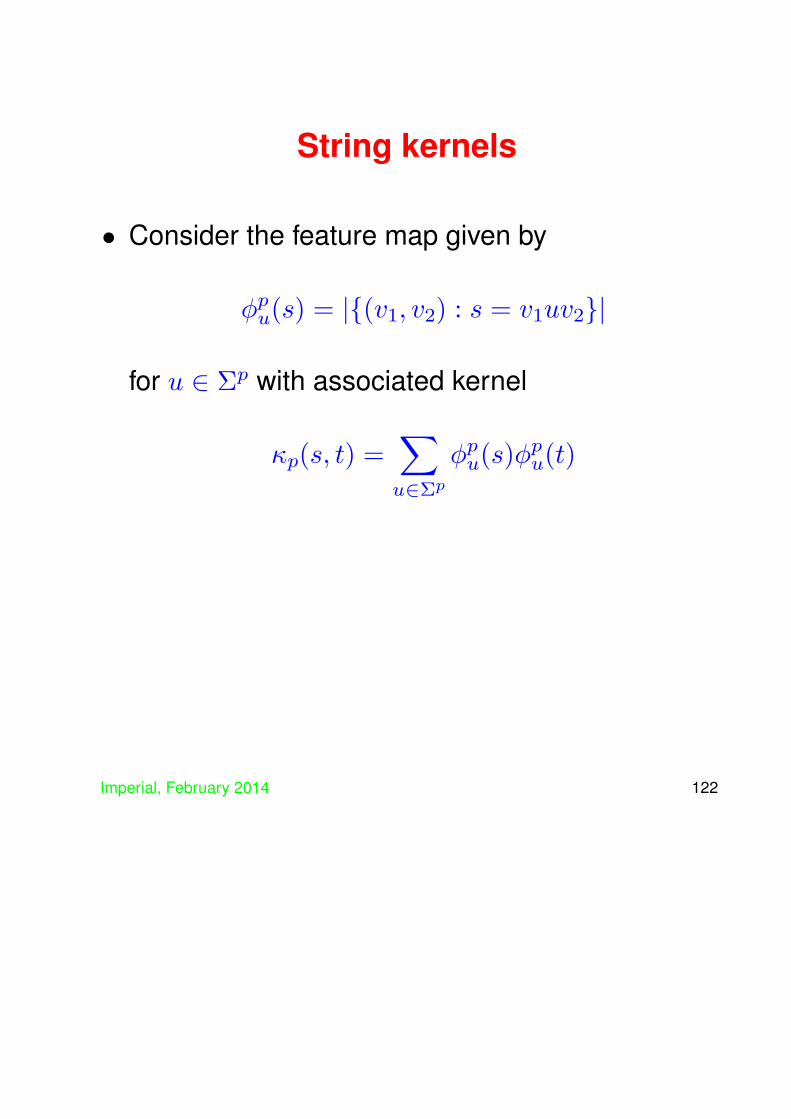
String kernels
• Consider the feature map given by
ϕpu(s) = |{(v1, v2) : s = v1uv2}|
for u ∈ Σp with associated kernel
κp(s, t) =∑u∈Σp
ϕpu(s)ϕ
pu(t)
Imperial, February 2014 122

String kernels
• Consider the following two sequences:
s ="statistics"t ="computation"
The two strings contain the following substringsof length 3:
"sta", "tat", "ati", "tis","ist", "sti", "tic", "ics""com", "omp", "mpu", "put","uta", "tat", "ati", "tio", "ion"
and they have in common the substrings "tat"and "ati", so their inner product would beκ (s, t) = 2.
Imperial, February 2014 123

Trie based p-spectrum kernels
• Computation organised into a trie with nodesindexed by substrings – root node by emptystring ϵ.
• Create lists of substrings at root node:
Ls(ϵ) = {(s(i : i+ p− 1), 0) : i = 1, |s| − p+ 1}
Similarly for t.
• Recursively through the tree: if Ls(v) and Lt(v)both not empty:for each (u, i) ∈ L∗(v) add (u, i + 1) to listL∗(vui+1)
• At depth p increment global variable kerninitialised to 0 by |Ls(v)||Lt(v)|.
Imperial, February 2014 124

Gap weighted string kernels
• Can create kernels whose features are allsubstrings of length p with the feature weightedaccording to all occurrences of the substring asa subsequence:
ϕ ca ct at ba bt cr ar br
cat λ2 λ3 λ2 0 0 0 0 0car λ2 0 0 0 0 λ3 λ2 0bat 0 0 λ2 λ2 λ3 0 0 0bar 0 0 0 λ2 0 0 λ2 λ3
• This can be evaluated using a dynamicprogramming computation over arrays indexedby the two strings.
Imperial, February 2014 125

Tree kernels
• We can consider a feature mapping for treesdefined by
ϕ : T 7−→ (ϕS(T ))S∈I
where I is a set of all subtrees and ϕS(T ) countsthe number of co-rooted subtrees isomorphic tothe tree S.
• The computation can again be performedefficiently by working up from the leaves of thetree integrating the results from the children ateach internal node.
• Similarly we can compute the inner product in thefeature space given by all subtrees of the giventree not necessarily co-rooted.
Imperial, February 2014 126

Probabilistic model kernels
• There are two types of kernels that can bedefined based on probabilistic models of thedata.
• The most natural is to consider a class of modelsindex by a model class M : we can then definethe similarity as
κ(x, z) =∑m∈M
P (x|m)P (z|m)PM(m)
also known as the marginalisation kernel.
• For the case of Hidden Markov Models thiscan be again be computed by a dynamicprogramming technique.
Imperial, February 2014 127
Probabilistic model kernels
• Pair HMMs generate pairs of symbols and undermild assumptions can also be shown to give riseto kernels that can be efficiently evaluated.
• Similarly hidden tree generating models of data,again using a recursion that works upwards fromthe leaves.
Imperial, February 2014 128

Fisher kernelsFisher kernels are an alternative way of definingkernels based on probabilistic models.
• We assume the model is parametrised accordingto some parameters: consider the simpleexample of a 1-dim Gaussian distributionparametrised by µ and σ:
M =
{P (x|θ) = 1√
2πσexp
(−(x− µ)
2
2σ2
): θ = (µ, σ) ∈ R2
}.
• The Fisher score vector is the derivative of thelog likelihood of an input x wrt the parameters:
logL(µ,σ) (x) = −(x− µ)2
2σ2− 1
2log (2πσ) .
Imperial, February 2014 129
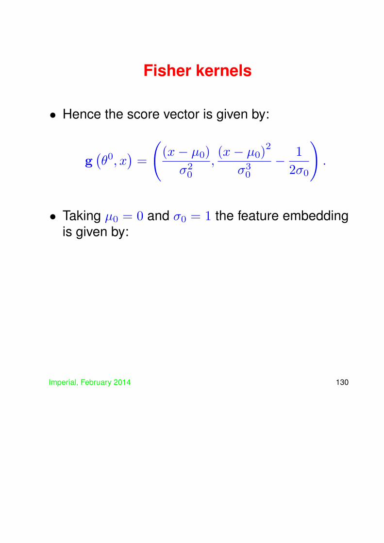
Fisher kernels
• Hence the score vector is given by:
g(θ0, x
)=
((x− µ0)
σ20
,(x− µ0)
2
σ30
− 1
2σ0
).
• Taking µ0 = 0 and σ0 = 1 the feature embeddingis given by:
Imperial, February 2014 130

Fisher kernels
−2 −1.5 −1 −0.5 0 0.5 1 1.5 2−0.5
0
0.5
1
1.5
2
2.5
3
3.5
−2 −1.5 −1 −0.5 0 0.5 1 1.5 2−0.5
0
0.5
1
1.5
2
2.5
3
3.5
Imperial, February 2014 131

Fisher kernels
Can compute Fisher kernels for various modelsincluding
• ones closely related to string kernels
• Hidden Markov Models
Imperial, February 2014 132

ConclusionsKernel methods provide a general purpose toolkitfor pattern analysis
• kernels define flexible interface to the dataenabling the user to encode prior knowledge intoa measure of similarity between two items – withthe proviso that it must satisfy the psd property.
• composition and subspace methods providetools to enhance the representation: normalisation,centering, kernel PCA, kernel Gram-Schmidt,kernel CCA, etc.
• algorithms well-founded in statistical learningtheory enable efficient and effective exploitationof the high-dimensional representations toenable good off-training performance.
Imperial, February 2014 133

Where to find out more
Web Sites: www.support-vector.net (SV Machines)
www.kernel-methods.net (kernel methods)
www.kernel-machines.net (kernel Machines)
www.neurocolt.com (Neurocolt: lots of TRs)
www.pascal-network.org
References
[1] N. Alon, S. Ben-David, N. Cesa-Bianchi, and D. Haussler.Scale-sensitive Dimensions, Uniform Convergence, andLearnability. Journal of the ACM, 44(4):615–631, 1997.
Imperial, February 2014 134

[2] M. Anthony and P. Bartlett. Neural Network Learning:Theoretical Foundations. Cambridge University Press,1999.
[3] M. Anthony and N. Biggs. Computational LearningTheory, volume 30 of Cambridge Tracts in TheoreticalComputer Science. Cambridge University Press, 1992.
[4] M. Anthony and J. Shawe-Taylor. A result of Vapnik withapplications. Discrete Applied Mathematics, 47:207–217, 1993.
[5] K. Azuma. Weighted sums of certain dependent randomvariables. Tohoku Math J., 19:357–367, 1967.
[6] P. Bartlett and J. Shawe-Taylor. Generalizationperformance of support vector machines and otherpattern classifiers. In B. Scholkopf, C. J. C. Burges,and A. J. Smola, editors, Advances in Kernel Methods— Support Vector Learning, pages 43–54, Cambridge,MA, 1999. MIT Press.
[7] P. L. Bartlett. The sample complexity of patternclassification with neural networks: the size of theweights is more important than the size of the network.
Imperial, February 2014 135
IEEE Transactions on Information Theory, 44(2):525–536, 1998.
[8] P. L. Bartlett and S. Mendelson. Rademacher andGaussian complexities: risk bounds and structuralresults. Journal of Machine Learning Research, 3:463–482, 2002.
[9] S. Boucheron, G. Lugosi, , and P. Massart. A sharpconcentration inequality with applications. RandomStructures and Algorithms, pages vol.16, pp.277–292,2000.
[10] O. Bousquet and A. Elisseeff. Stability andgeneralization. Journal of Machine Learning Research,2:499–526, 2002.
[11] N. Cristianini and J. Shawe-Taylor. An introduction toSupport Vector Machines. Cambridge University Press,Cambridge, UK, 2000.
[12] Y. Freund and R. E. Schapire. A decision-theoreticgeneralization of on-line learning and an application toboosting. In Computational Learning Theory: Eurocolt’95, pages 23–37. Springer-Verlag, 1995.
Imperial, February 2014 136

[13] W. Hoeffding. Probability inequalities for sums ofbounded random variables. J. Amer. Stat. Assoc.,58:13–30, 1963.
[14] M. Kearns and U. Vazirani. An Introduction toComputational Learning Theory. MIT Press, 1994.
[15] V. Koltchinskii and D. Panchenko. Rademacherprocesses and bounding the risk of function learning.High Dimensional Probability II, pages 443 – 459, 2000.
[16] J. Langford and J. Shawe-Taylor. PAC bayes andmargins. In Advances in Neural Information ProcessingSystems 15, Cambridge, MA, 2003. MIT Press.
[17] M. Ledoux and M. Talagrand. Probability in BanachSpaces: isoperimetry and processes. Springer, 1991.
[18] C. McDiarmid. On the method of bounded differences. In141 London Mathematical Society Lecture Notes Series,editor, Surveys in Combinatorics 1989, pages 148–188.Cambridge University Press, Cambridge, 1989.
[19] R. Schapire, Y. Freund, P. Bartlett, and W. SunLee. Boosting the margin: A new explanation for theeffectiveness of voting methods. Annals of Statistics,
Imperial, February 2014 137
1998. (To appear. An earlier version appeared in:D.H. Fisher, Jr. (ed.), Proceedings ICML97, MorganKaufmann.).
[20] J. Shawe-Taylor, P. L. Bartlett, R. C. Williamson,and M. Anthony. Structural risk minimization overdata-dependent hierarchies. IEEE Transactions onInformation Theory, 44(5):1926–1940, 1998.
[21] J. Shawe-Taylor and N. Cristianini. On the generalisationof soft margin algorithms. IEEE Transactions onInformation Theory, 48(10):2721–2735, 2002.
[22] J. Shawe-Taylor and N. Cristianini. Kernel Methodsfor Pattern Analysis. Cambridge University Press,Cambridge, UK, 2004.
[23] J. Shawe-Taylor, C. Williams, N. Cristianini, and J. S.Kandola. On the eigenspectrum of the gram matrixand its relationship to the operator eigenspectrum. InProceedings of the 13th International Conference onAlgorithmic Learning Theory (ALT2002), volume 2533,pages 23–40, 2002.
[24] M. Talagrand. New concentration inequalities in product
Imperial, February 2014 138

spaces. Invent. Math., 126:505–563, 1996.[25] V. Vapnik. Statistical Learning Theory. Wiley, New York,
1998.[26] V. Vapnik and A. Chervonenkis. Uniform convergence of
frequencies of occurence of events to their probabilities.Dokl. Akad. Nauk SSSR, 181:915 – 918, 1968.
[27] V. Vapnik and A. Chervonenkis. On the uniformconvergence of relative frequencies of events to theirprobabilities. Theory of Probability and its Applications,16(2):264–280, 1971.
[28] Tong Zhang. Covering number bounds of certainregularized linear function classes. Journal of MachineLearning Research, 2:527–550, 2002.
Imperial, February 2014 139