Kepler Monitoring of an L Dwarf I. The Photometric Period

and White Light Flares

John E. Gizis,1 Adam J. Burgasser, 2 Edo Berger,3 Peter K. G. Williams,3 Frederick J.

Vrba,4 Kelle L. Cruz,5,6 Stanimir Metchev7

ABSTRACT

We report on the results of fifteen months of monitoring the nearby field

L1 dwarf WISEP J190648.47+401106.8 (W1906+40) with the Kepler mission.

Supporting observations with the Karl G. Jansky Very Large Array and Gemini

North telescope reveal that the L dwarf is magnetically active, with quiescent

radio and variable Hα emission. A preliminary trigonometric parallax shows

that W1906+40 is at a distance of 16.35+0.36−0.34 pc, and all observations are con-

sistent with W1906+40 being an old disk star just above the hydrogen-burning

limit. The star shows photometric variability with a period of 8.9 hours and

an amplitude of 1.5%, with a consistent phase throughout the year. We infer

a radius of 0.92 ± 0.07RJ and sin i > 0.57 from the observed period, luminos-

ity (10−3.67±0.03L⊙), effective temperature (2300 ± 75K) , and v sin i (11.2 ± 2.2

km s−1). The light curve may be modeled with a single large, high latitude dark

spot. Unlike many L-type brown dwarfs, there is no evidence of other variations

at the & 2% level, either non-periodic or transient periodic, that mask the un-

derlying rotation period. We suggest that the long-lived surface features may

be due to starspots, but the possibility of cloud variations cannot be ruled out

without further multi-wavelength observations. During the Gemini spectroscopy,

1Department of Physics and Astronomy, University of Delaware, Newark, DE 19716, USA

2Center for Astrophysics and Space Science, University of California San Diego, La Jolla, CA 92093, USA

3Harvard-Smithsonian Center for Astrophysics, 60 Garden Street, Cambridge, MA 02138, USA

4US Naval Observatory, Flagstaff Station, 10391 West Naval Observatory Road, Flagstaff, AZ 86001,

USA

5Department of Physics and Astronomy, Hunter College, City University of New York, 695 Park Avenue,

New York, NY 10065, USA

6Department of Astrophysics, American Museum of Natural History, Central Park West at 79th Street,

New York, NY 10025, USA

7Department of Physics and Astronomy, State University of New York, Stony Brook, NY 11794, USA

– 2 –

we observed the most powerful flare ever seen on an L dwarf, with an estimated

energy of 1.6 × 1032 ergs in white light emission. Using the Kepler data, we

identify similar flares and estimate that white light flares with optical/ultraviolet

energies of 1031 ergs or more occur on W1906+40 as often as 1-2 times per month.

Subject headings: brown dwarfs — stars: activity — stars: flare — stars: spots

— stars: individual: WISEP J190648.47+401106.8

1. Introduction

Dramatic changes in the spectra of ultracool dwarfs with Teff . 2300 K lead to their

classification as a distinct spectral type, the L dwarfs (Kirkpatrick et al. 1999; Martın et al.

1999). The L dwarf field population is a mix of old hydrogen-burning stars and young brown

dwarfs. The weakening of molecular features and reddening of broad-band colors compared

to M dwarfs are explained by the formation of condensates, or dust grains (see the review

by Kirkpatrick 2005). Early observations established that chromospheric activity weakens

in this spectral type range (Gizis et al. 2000), and it is now clear that magnetic activity

changes dramatically in character (see Berger et al. 2010; McLean et al. 2012). L0-L2 dwarfs

are cooler than the M dwarfs which show optical variations due to cool magnetic starspots

(Basri et al. 2011), but warmer than the L/T transition brown dwarfs that show mounting

evidence of infrared variations due to cloud inhomogeneties (Artigau et al. 2009; Radigan

et al. 2012; Buenzli et al. 2012). These considerations suggest that L dwarfs may show

variability due to changes in the condensate distribution (such as clouds, or holes in cloud

decks) and/or magnetic starspots. Because measurements of v sin i suggest all L dwarfs are

rapid rotators (Bailer-Jones 2004; Reiners & Basri 2008), rotational modulation is expected

to have periods of hours.

Optical (I-band) variations have been detected in many L dwarfs at the few percent

level (Bailer-Jones & Mundt 2001; Clarke et al. 2002; Gelino et al. 2002; Clarke et al. 2003;

Koen 2003, 2005, 2006; Lane et al. 2007) and usually attributed to inhomogenities in the

clouds. Although a few detected I-band signals were periodic and consistent with rotational

modulation, others were not, and characteristics seen in one observing run may be different

in another. Bailer-Jones & Mundt (2001) suggested that surface features in early L dwarfs

evolve on timescales of hours and “mask” the underlying rotation curve in I-band: A par-

ticularly interesting case was 2MASSW J1145572+231730 (hereafter 2M1145+23), an L1.5

dwarf with Hα emission (Kirkpatrick et al. 1999), which showed periods that did not match

the previous year’s observations (Bailer-Jones & Mundt 1999, 2001). Gelino et al. (2002)

found that at least seven, and perhaps up to twelve, of eighteen L dwarfs were variable at

– 3 –

I-band, but that most had non-periodic light-curves. The two observed periods were thought

to be much longer than the rotation rates. Koen (2006) reported that the L0 dwarf 2MASS

J06050196-22342270 had a consistent 2.4 hour period over three nights, but the amplitude

declined from 27 to 11 mmag. Both Bailer-Jones & Mundt (2001) and Gelino et al. (2002)

considered the balance of evidence favored cloud variations over sunspot-like starspots, al-

though some possible starspots have been noted in L dwarfs with Hα emission (Bailer-Jones

& Mundt 1999; Clarke et al. 2003). Lane et al. (2007) suggests that a three-hour periodicity

in the L3.5 2MASSW J0036159+182110 is due to starspots: Although this source is not

chromospherically active, it is radio active (Berger et al. 2005). These observations are all of

field L dwarfs; Caballero et al. (2004) did not find statistically significant variations in young

(σ Ori) early L-type brown dwarfs, but few percent variations would have been below the

detection threshold and warmer young brown dwarfs showed evidence of accretion.

Flares are another potential type of variability in ultra cool dwarfs, but only a few optical

flares in L dwarfs have been reported (Liebert et al. 2003; Schmidt et al. 2007; Reiners &

Basri 2008). As Schmidt et al. (2007) remark, only the Hα emission line has been seen in

these flares, and not the nearby helium emission lines seen in M dwarf flares. In a study of

M8-L3 dwarfs, Berger et al. (2010) placed a limit of . 0.04 hr−1 on the rate of flares that

increase the Hα line more than a factor of a few above the quiescent chromospehric emission

level. This rate is consistent with the estimated L dwarf flare duty cycle of ∼ 1−2% (Liebert

et al. 2003; Schmidt et al. 2007). In contrast, many strong flares have been observed in M7-

M9 dwarfs (Liebert et al. 1999; Martın & Ardila 2001; Rockenfeller et al. 2006; Stelzer et al.

2006; Schmidt et al. 2007), with other atomic emission lines and even white light continuum

emission in some cases. Their Hα flare duty cycle is also much higher, perhaps 5-7% (Gizis

et al. 2000; Schmidt et al. 2007). Notably, simultaneous radio-optical monitoring of two

M8.5 dwarfs found no temporal correlation between radio flares and Hα flares (Berger et al.

2008a,b).

The field L dwarf observations are intriguing, but the limitations of telescope scheduling

and ground-based observing make it difficult to reliably characterize L dwarf variability and

assess the relative contribution of periodic and non-periodic components. The discovery of

WISEP J190648.47+401106.8 (hereafter W1906+40, Gizis et al. 2011), a nearby L1 dwarf in

the Kepler Mission (Koch et al. 2010) field of view, has allowed us to obtain a 15 month long

time series from space. Although W1906+40 is much fainter (SDSS g, r, i = 22.4, 20.0, 17.4)

than the typical FGKM main sequence star targeted with Kepler, the achieved precision

of 7 mmags per observation compares favorably with ground-based data. We report on

the Kepler photometry and supporting multi-wavelength observations in Section 2, discuss

periodicity in Section 3, and discuss flares in Section 4.

– 4 –

2. Observations

2.1. Kepler Data

W1906+40 was observed with Kepler Director’s Discretionary Time (Program GO30101)

from 28 June 2011 to 27 June 2012 and with Guest Observer time (Program GO40004) from

28 June 2012 to 03 October 2012. Its parameters are listed in Table 1. It was assigned a

new name for each quarter: KIC 100003560 (Quarter 10), KIC 100003605 (Quarter 11), KIC

100003905 (Quarter 12), KIC 100004035 (Quarter 13), and KIC 100004076 (Quarter 14). The

target was observed in long cadence mode (Jenkins et al. 2010b), providing 30 minute obser-

vations, for the full time period and also in one-minute short cadence mode (Gilliland et al.

2010) during Quarter 14. For each observation, the Kepler pipeline (Jenkins et al. 2010a)

provides the pixel data, the time (t = BJD− 2454833.0, or mission days), the aperture flux

(SAP Flux), the uncertainty, and a corrected aperture flux (PDCSAP Flux), which is meant

to correct instrumental drifts (Stumpe et al. 2012). After excluding data flagged as bad

(Quality Flag > 0), there are 18,372 long cadence measurements. The pipeline-estimated

noise levels are 0.5%. For Quarters 10 and 14, we adopt the PDCSAP Flux photometry.

These quarters used an aperture of nine pixels. The spacecraft is rotated between quarters,

so W1906+40 was observed on four different detectors with different focus and different aper-

tures. The default pipeline analysis used larger apertures for Quarters 11-13, which resulted

in noisier photometry. Quarter 13’s PDCSAP Flux is very low (< 100 counts per second),

which we found is due to two negative (bad) pixels included in the aperture. Smaller aper-

tures also reduce the possibility of contamination by nearby background stars. We therefore

adopted smaller apertures of six pixels for Quarters 11 and 12 and four pixels for Quarter 10

using the PyKE tool kepextract.1 Instrumental drifts for these three quarters were removed

with third-order polynomial fits. Kepler photometry is not calibrated in any absolute sense

since such calibration is not needed to meet the primary mission goals, so we divided each

quarter’s data by the median count rate for that quarter.

The Kepler data show a strong peak in the periodogram at a period of 0.3702 days. We

emphasize that this period is present in each quarter, and in both the pipeline photometry

and our revised (smaller aperture) photometry. This 8.9 hour period is consistent with

the rotation period distribution deduced for early L dwarfs by their v sin i measurements

(Reiners & Basri 2008). We fit a sine curve to the first year’s data with a Markov Chain

Monte Carlo (MCMC) analysis and find the period is 0.370152 ± 0.000002 days with an

amplitude of 0.00763± 0.00006 (8.3 mmag). The peak-to-peak variation is twice this (1.5%,

1PyKE is available through the Kepler Mission contributed software webpage:

http://keplergo.arc.nasa.gov/PyKE.shtml

– 5 –

or 16 mmag). Fitting each quarter separately yields periods of 0.37015± 0.00005. The full

phased dataset with sine curve is shown in Figure 1. Excluding the small number of outliers,

whose nature are discussed in Section 4, the standard deviation about the fit is 0.65%, or 7

mmag. We adopt this as the noise level of the measurements, as it is only a slight increase

over the expected value (0.5%) and there are other possible noise sources in the Kepler

instrument (Caldwell et al. 2010), though real intrinsic variations may contribute. Figure 2

shows four days of data; this region happens to include our radio observations (Section 2.3)

and a possible flare (Section 4.2).

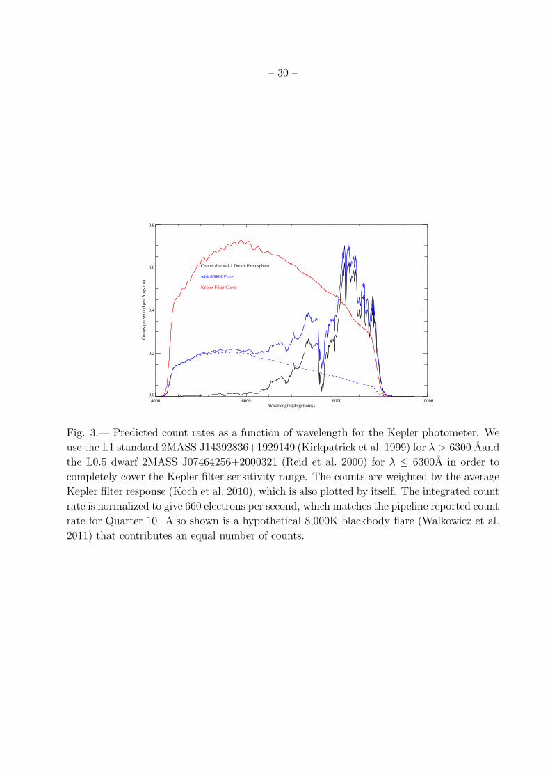
It can be useful to discuss flares in terms of energies instead of relative counts. Walkowicz

et al. (2011) and Maehara et al. (2012) have estimated the energy of white light flares on

G, K and M dwarfs observed by Kepler by approximating the flare as a 10,000K blackbody.

The Kepler Mission filter is similar to g,r, and i combined (Koch et al. 2010): As illustrated

in Figure 3, the L dwarf photosphere contributes mainly at the very reddest wavelengths,

but hot flares will contribute through the entire filter. Indeed, the effective wavelength for

the Kepler photometry for W1906+40 is 7990A rather than ∼ 6200A for hot sources. In

Table 2, we present energy calculations of hypothetical flares that have the same observed

count rate as W1906+40, assuming the flares radiate isotropically. We use the i magnitude,

the distance derived in Section 2.2, and the L1 dwarf spectrum shown in Figure 3 to estimate

that the L dwarf luminosity is 1.4 × 1028 erg s−1 in the wavelength range 4370Ato 8360A.

The blackbody energies for equal count rates are 50% higher because the energy per photon

is higher, 2.1 × 1028 erg s−1. Thus, to double the observed Kepler count rate, one needs a

flare of 1.3 × 1030 erg (over that wavelength range) during a short cadence exposure and

3.8 × 1031 erg during a long cadence exposure. Most of the flare energy will be emitted at

shorter optical and ultraviolet wavelengths. The corresponding bolometric luminosities for

the blackbodies are 4.4 to 6.4 erg s−1. Real flares are not blackbodies, so we also estimated

the total luminosities by consulting Table 6 of Hawley & Pettersen (1991), which gives

energies from 1200Ato 8045Afor the impulsive and gradual phases of great flare of 12 April

1984 on AD Leo. The results are close to the blackbody approximations.

2.2. Optical and Near-Infrared Observations

W1906+40 was observed with the Gemini Multi-Object Spectrograph (Hook et al. 2004)

on the Gemini North telescope (Program GN-2012A-Q-37). The R831 grating, OG515 order

blocking filter, and 1.0 arcsecond slit were used to yield wavelength coverage 6276A to 8393

A, with two small gaps between detectors that were interpolated over. We obtained sixteen

600-second exposures on UT Date 24 July 2012, twenty-five on 29 July 2012, and six on

– 6 –

UT Date 8 August 2012. The flux calibration star BD+28 4211 was observed on 29 July

2012. The data were bias-subtracted, flat-fielded, wavelength-calibrated, extracted and flux-

calibrated in the standard way using the Gemini gmos package in IRAF. A small correction

was then applied to bring the spectra in agreement with the i-band magnitude.

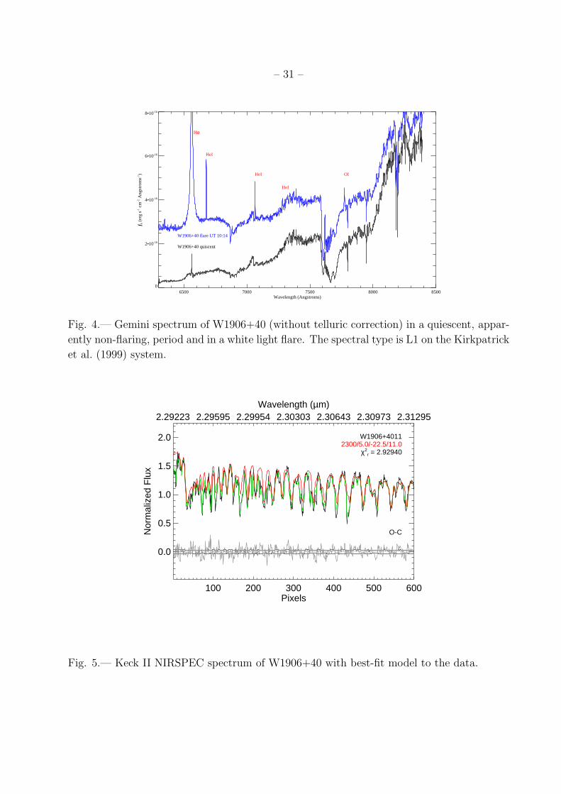
We compared the Gemini spectra to the spectral type standards defined by Kirkpatrick

et al. (1999) and find that W1906+40 is spectral type L1 (Figure 4.) It is not a low gravity

L dwarf (Cruz et al. 2009). We see no evidence for lithium absorption in any of the spectra.

The L1 optical spectral type agrees with the L1 near-infrared spectral type derived in the

discovery report. Hα is variable on all nights but detected in emission in all spectra. On 24

July the Hα emission equivalent width increased from 0.5A at the beginning of observations

to 7.5A at the end. On 29 July 2012, the Hα emission begins at 2.8A, but is then dominated

by flares, discussed further in Section 4.1, as seen in Figure 4. On 8 August, the first five

spectra have an equivalent width of 2.5-3.0 A, but the last increases to 6.5A. The average

non-flare Hα equivalent width is 4A. The flares on 29 July overwhelm the small periodic

signal, so we defer any attempt to identify small photospheric changes on the other nights

to a future paper when additional simultaneous ground-based and Kepler data are available.

W1906+40 was observed in clear and dry conditions on 10 September 2011 (UT) with

the Keck II NIRSPEC near-infrared echelle spectrograph (McLean et al. 2000), as part of an

ongoing search for radial velocity variables among nearby L dwarfs (Burgasser et al. 2012).

The source was observed using the high-dispersion mode, N7 filter and 0.′′432×12′′ slit to

obtain 2.00–2.39 µm spectra over orders 32–38 with λ/∆λ = 20,000 (∆v = 15 km s−1) and

dispersion of 0.315 A pixel−1. Two 120 s exposures were obtained in two nods separated by

7′′ along the slit. We also observed the A0 V calibrator HD 192538 (V = 6.47) in the same

setup for telluric correction and flux calibration, and internal quartz flatfield and NeArXeKr

arc lamps for pixel response and wavelength calibration, respectively.

Spectral data were extracted from the images using the REDSPEC package2, and we

focused our analysis on order 33 which samples the strong CO band around 2.3 µm (Blake

et al. 2008). We used REDSPEC and associated routines to perform pixel-response cali-

bration, background subtraction, order identification, image rectification, and extraction of

raw counts for both target and A0 V star. We also obtained an initial linear wavelength

calibration using the arc lamp images, but performed no telluric or flux calibration. We

then used these data to perform a forward-modeling analysis similar to that described in

Blake et al. (2010). Our full methodology will be presented in a future paper, but in brief

2REDSPEC was developed for NIRSPEC by S. Kim, L. Prato, and I. McLean; see

http://www2.keck.hawaii.edu/inst/nirspec/redspec/index.html.

– 7 –

we explored a parameterized model of the raw spectrum

S[p] = {(M [p(λ,RV )]⋆K)×T [p(λ)]α×C[p]} ⋆LSF (1)

through Markov Chain Monte Carlo (MCMC) methods. Here, M is a synthetic model

chosen from the BT-Settled set of Allard et al. (2011), spanning 1800 K ≤ Teff ≤ 2500 K

in 100 K steps and 4.5 ≤ log g ≤ 5.5 (cgs) in 0.5 dex steps, and sampled at a resolution

of 300,000 (∆v = 1 km s−1); p(λ) is the conversion function from wavelength to pixel,

modeled as a third-order polynomial; RV is the barycentric radial velocity of the star; K is

the rotational broadening kernel defined by Gray (1992) which depends on v sin i; T[λ] is the

telluric absorption spectrum, adopted from the solar absorption spectral atlas of Livingston

& Wallace (1991); α scales T[λ] to match the observed telluric absorption; C is the flux

calibration function, modeled as a second-order polynomial; LSF is the spectrograph line

spread function, modeled as a Gaussian with width σG; and ⋆ denotes convolution. To

facilitate rapid exploration of this 11-component parameter space, we performed the rotation

convolution on all of the models in advance, sampling 5 km s−1≤ v sin i ≤ 100 km s−1in

1 km s−1steps. Parameters were initiated by first fitting the A0 V observation; we then fit

the W1906+40 spectrum using MCMC chains of length 1000 for each of the spectral models

deployed (Teff and log g), following standard procedures (e.g., Ford 2005) and using χ2 as

our cost function .

Figure 5 shows our best-fit model to the data, with Teff = 2300 K, log g = 5.0 dex,

heliocentric radial velocity of −22.5 km s−1(assuming a barycentric motion of −10.7 km s−1)

and v sin i = 11 km s−1. The fit is good (reduced χ2 = 2.9), and the strong blend of both

stellar and telluric absorption features provides a robust framework for constraining both

radial and rotational velocities. To determine estimates of each, we marginalized all of the

chains for each parameter p using a probability function based on the F-test statistic

〈p〉 =all chains∑

i

pi℘i (2)

σ2p =

(

all chains∑

i

p2i℘i

)

− 〈p〉2 (3)

where the probability function ℘ for each chain was determined from the F-test probability

distribution function

℘i ∝ 1− F (χ2i /min({χ2}), ν, ν) (4)

(see Burgasser et al. 2010) with min({χ2}) being the minimum χ2 (best-fitting model), ν the

degrees of freedom (# pixels −# parameters), and enforcing∑

℘i = 1. From this calculation

we determined RV = −22.6±0.4 km s−1 and v sin i = 11.2±2.2 km s−1 for W1906+40. The

– 8 –

fitted Teff is consistent with other L dwarf studies (see the reviews of Chabrier & Baraffe

2000; Kirkpatrick 2005), so we estimate the uncertainty in Teff as ±75K.

The parallax and proper motion were obtained with the ASTROCAM (Fischer et al.

2003) imager at the 1.55-m telescope of the U.S. Naval Observatory, using the astrometric

observing and reduction principles described in Vrba et al. (2004). Observations in J-band

were obtained on 27 nights over the course of 1.23 years. A reference frame employing 16

stars with a range of apparent J magnitude of 11.8-14.6 was employed. The conversion

from relative to absolute parallax was based on using both 2MASS and SDSS photometry

to determine a mean distance of the reference frame stars of 2.20 mas. We caution that this

is a preliminary parallax since, even with an excellent reference frame and a location in the

sky giving a significant parallax factor in declination, an observational time baseline of 1.23

years is not sufficient to completely separate parallax and proper motion. This object will be

on the USNO infrared parallax program for the next 2-3 years to establish a final parallax.

This distance (16.35+0.36−0.34 pc) is in excellent agreement with that derived in the discovery

paper (16.6± 1.9 pc) assuming the object to be single. If there is a unresolved companion,

it is therefore unlikely to contribute significantly to the Kepler photometry. As shown in the

Kirkpatrick (2005) review, an L1 dwarf like W1906+40 is most likely a hydrogen-burning

star with age & 300 Myr. The observed tangential velocity is greater than the median (30

km s−1) for L1 dwarfs (Faherty et al. 2009), supporting an old age and stellar status. Both

integrating the W1906+40 near-infrared spectrum and optical to mid-infrared photometry

and comparison to other L1 dwarfs (Golimowski et al. 2004) gives BCK = 3.22± 0.06, and

therefore logL/L⊙ = −3.67±0.03. Overall, our optical and near-infrared observations show

that W1906+40 is a typical L1 dwarf, though the Hα and rotation rate places it in the

more chromospherically active and slowly rotating half of the population. If the L dwarf

rotation-age relation suggested by Reiners & Basri (2008) is correct, W1906+40 would be

older than 5 Gyr.

2.3. Radio Observations

W1906+40 was observed with the Karl G. Jansky Very Large Array (VLA)3 for three

hours starting at 2012 Feb 23.46 UTC (Project 12A-088). The total observing bandwidth

was 2048 MHz, with two subbands centered at 5000 and 7100 MHz and divided into 512

channels each. Standard calibration observations were obtained, with 3C286 serving as

3The VLA is operated by the National Radio Astronomy Observatory, a facility of the National Science

Foundation operated under cooperative agreement by Associated Universities, Inc.

– 9 –

the flux density scale and bandpass calibrator and the quasar J1845+4007 (4◦ from W1906)

serving as the phase reference source. The total integration time on W1906 was 120 minutes.

The VLA data were reduced using standard procedures in the CASA software system

(McMullin et al. 2007). Radiofrequency interference was flagged manually. After calibration,

a deep image of 2048×2048 pixels, each 1×1 arcsec, was created. The imaging used multi-

frequency synthesis (Sault & Wieringa 1994) and CASA’s multifrequency CLEAN algorithm

with two spectral Taylor series terms for each CLEAN component; this approach models both

the flux and spectral index of each source. The rms residual of the deconvolution process

around W1906 was 2.9 µJy bm−1.

W1906+40 is detected at the eight-sigma level with flux density 23.0 ± 4.1 µJy at a

mean observing frequency of 6.05 GHz. This corresponds to νLν = (4.5± 0.9)× 1022 erg s−1

with spectral index (Sν ∝ να) α = −2.0 ± 1.4. The mean time of the observation is 23 Feb

2012 12:40:50 UTC which equals Kepler mission time 1148.026. This corresponds to phase

0.91 in Figure 1, close to the minimum in the Kepler light curve. The time series is shown in

Figure 2. We searched for variability in W1906+40 by using the deep CLEAN component

model to subtract all other detectable sources from the visibility data, then plotting the

real component of the mean residual visibility as a function of time, rephasing the data to

the location of W1906. No evidence for variability was seen. We imaged the LL and RR

polarization components separately and found no evidence for significant circular polarization

of the emission fromW1906+40. W1906+40 is just the sixth L/T dwarf detected in quiescent

radio emission (Berger 2002, 2006; Berger et al. 2009; Burgasser et al. 2013; Williams et al.

2013).

2.4. Mid-Infrared (WISE) data

The W1906+40 discovery paper was based on the Preliminary Wide Field Infrared Ex-

plorer (WISE, Wright et al. 2010) data release. It appears as source WISE J190648.47+401106.8

in the final WISE All-Sky Source Catalog. The source was scanned 28 times over 1.9 days

in April 2010 as part of the main WISE Mission and again 34 times over 4.3 days in Oc-

tober 2010 in the Post-Cryo mission. We find that in the WISE All-Sky Single Exposure

(L1b) Source Table and WISE Preliminary Post-Cryo Single Exposure (L1b) Source Tables,

W1 is consistent between and within the two epochs, but the source apparently brightened

from W2= 11.23 ± 0.02 in April 2010 to a mean W2= 11.12 ± 02 in October (with indi-

vidual uncertainties ±0.03 magnitudes.) The October data also shows more scatter in W2

than expected, but higher precision mid-infrared observations would be needed to confirm

variability. The WISE data are more than 680 periods before the beginning of the Kepler

– 10 –

data.

3. Photometric Variability

3.1. Radius and Inclination

The radius and inclination of W1906+40 are important parameters in interpreting the

Kepler light curve. We can constrain them both using our observations. First, the radius is a

function of the observed distance (and thereby the luminosity) and our effective temperature

fit:

R = 0.90± 0.03RJ

(

2300K

Teff

)2(

d

16.35pc

)

(5)

The uncertainty of 3% includes the uncertainty in the bolometric correction and pho-

tometry but not parallax or temperature uncertainty. Second, assuming the photometric

period is the rotation period, we can also constrain the radius and inclination with our

spectroscopic v sin i:

R sin i = 0.80RJ

(

P

0.37015 d

)(

v sin i

11.2 kms−1

)

(6)

The uncertainty in this value is 20% due to the v sin i uncertainty. Combining this

constraint with Equation 5 suggests i ≈ 60◦, but a range of inclinations are possible. Since

the period is so strongly constrained, we can infer the posterior probability using three ob-

servations for the data (luminosity, effective temperature, and v sin i) and a three parameter

model (luminosity, radius, and sin i). Our priors are flat in luminosity and radius, but pro-

portional to sin i on geometric grounds. Using an MCMC chain of one million steps, and

discarding a burn-in of one thousand steps, we find the posterior probability distribution

shown in Figure 6. The inferred radius is R = 0.92 ± 0.07RJ . At the 95% confidence level,

we find that sin i > 0.59, with the median value sin i = 0.83 and most likely value sin i = 0.90.

The inferred radius is consistent with theoretical predictions of 0.8 .< R . 1.0RJ (Chabrier

et al. 2000; Burrows et al. 2011).

– 11 –

3.2. Spot models

The most striking aspect of the Kepler light curve is that it has a consistent phase

for over a year. Furthermore, while we cannot rule out deviations from a sine function or

small changes in the shape, it appears that the light curve has no flat portion. The simplest

explanation is that the rotating dwarf has a single feature (darker or brighter than the

surrounding photosphere) that is always in view. To explore this possibility, we model the

first year of data using the circular spot equations of Dorren (1987), which we implemented in

Python with an MCMC code. We assumed linear limb darkening coefficients of 0.9 based on

the predictions of Claret (1998) and Claret & Bloemen (2011). Many solutions are possible,

and generally we can find single dark spot models with χ2 similar to the sine models. Some

possible solutions with completely dark spots with sin i consistent with Figure 6 and are

listed in Table 3. Solutions with i ≈ 80◦ can be found, but they require a larger spot. The

different light curve during Quarter 13 could be explained in large part in the single circular

dark spot model by increasing the spot size (to ∼ 13◦ for i = 60◦), or by lowering the

latitude (to ∼ 70◦ for i = 60◦). While attributing a long-lived feature to a single “spot” is

attractive, it could also be modeled in other ways, such as multiple large dark spots at lower

latitudes. An intriguing alternative spot model that does not favor large circumpolar spots

was presented for active dwarfs by Alekseev & Gershberg (1996). In this “zonal model,” it

is assumed that a large number of small spots together form large dark bands symmetric

around the equator. This naturally produces sinusoidal light curve even at sin i ≈ 1 without

requiring us to be viewing polar spots.

The physical cause of the putative large spot at high latitude (or even multiple spots

at low latitudes) might be a magnetic starspot (i.e., a region of cooler photosphere due to

magnetic fields) or an cloud structure. Jupiter’s Great Red Spot would produce a strong

periodic signal at 9.9 hours even in unresolved data (Gelino & Marley 2000), though a single

spot on W1906+40 would be at much higher latitude. Gelino et al. (2002) comment that

small holes in a cloud layer would form bright (I-band) spots “similar to the ‘5 µm hot spots’

of Jupiter.” These might be distributed according to the zonal model. Harding et al. (2011)

argue for a “magnetically-driven auroral process” to produce optical variations in some ultra

cool dwarfs. We cannot determine whether the features are brighter or darker with the

single-band Kepler data, so all of these possibilities are plausible. It is worth considering

whether chromospheric emission line variations would explain the Kepler periods. Varying

Hα emission from zero to ten Angstroms equivalent width, even with associated bluer Balmer

lines, would only produce a signal of ∼ 0.0015%, an order of magnitude too small to explain

our data.

The stability of the period and amplitude makes a striking contrast with the L dwarf

– 12 –

observations discussed in the Introduction. Besides the stable 8.9 hour period, we find no

evidence of other periods, transient or not, in the data. To search for other periods of

hours to days, we have calculated periodograms for every three, five, and ten day period

and found no other significant period in any of them. The long-term drifts we removed

were typically 1%, and only reached 6% during quarter 11, and these are consistent with the

drifts in bright stars corrected by the PDC pipeline process. Although intrinsic slow changes

in W1906+40 on timescales of months might be removed, it is likely that a strong signal,

like the ∼ 30 day period M dwarf GJ 4099 (KIC 414293, Basri et al. 2011), would still be

detected. Variations on timescales less than a week that are & 1% would be detected. We

conclude that the various “masking” periods and non-periodic variations reported in other

L dwarfs at amplitudes > 2%, and attributed to condensate cloud inhomogeneties, are not

present in W1906+40. On the other hand, variations . 1% can be plausibly be attributed to

noise, but could also be due to real variations. (The data shown in Figure 2 are suggestive,

and typical.)

If the short-lived variability observed on non-active ultracool dwarfs is associated with

condensate clouds, perhaps the long-lived periodic feature on this active L dwarf is associated

with different, possibly magnetic, phenomena. A number of studies (Berger et al. 2005;

Hallinan et al. 2006, 2008; Berger et al. 2009; McLean et al. 2011) have suggested that some

ultracool dwarfs have stable magnetic large-scale topologies, like dipoles or quadrupoles.

This could result in a large high-latitude feature. Hussain (2002) reviewed starspot lifetimes:

While starspots on single, young main-sequence stars have typical lifetimes of a month, other

types of starspots can have lifetimes of years or decades. Furthermore, an active longitude

may remain more heavily spotted for years, even as individual spots come and go on shorter

timescales. Of course, as Lane et al. (2007) remark, a cooler starspot on an L dwarf might

have different cloud properties than the normal photosphere.

4. Flare Analysis

4.1. Spectroscopy and photometry of the 29 July 2012 flares

After the first forty minutes of Gemini data on 29 July 2012 show relatively quiescent

Hα emission, the subsequent spectra are dominated by a series of flares characterized by

strong emission lines and a blue continuum. The first flare is in the ten minute exposure

beginning at UT 08:29:28, followed by a more powerful “main” flare at UT 10:14:15 (shown

in Figure 4. Both of these flares are detected in the Kepler short cadence photometry: the

first flare peaks at mission time 1304.8597 and the atomic emission lines as a function of

time throughout the night are shown in Figure 8 along with the simultaneous Kepler short

– 13 –

cadence photometry.4 The Kepler light curve is in good agreement with the appearance of

the spectroscopic white light continuum. Even with multi wavelength data at high time

resolution (see Gershberg 2005), flare spectra have proven to be challenging to interpret.

Most notably, this L1 dwarf is able to produce a white light flare that is similar to that

observed in M dwarf flare stars. Indeed, the flare spectrum is very similar to Fuhrmeister

et al. (2008)’s flare in the M6 dwarf CN Leo (Wolf 359), including the white light, broad

Hα, and atomic emission lines. The flare also resembles the most powerful observed M7

(Schmidt et al. 2007) and M9 (Liebert et al. 1999) dwarf flares, demonstrating continuity in

the flare properties across the M/L transition. The white light and emission line light curves

are qualitatively very similar to the 28 March 1984 AD Leo flare described by Houdebine

(1992) as “impulsive/gradual.”

The main flare shows both atomic emission lines and continuum emission with a blue

slope. The higher time resolution photometry shows that the flare began four minutes into

the Gemini UT 10:14:15 exposure, and reached its Kepler maximum in the final two minutes.

The “white light” flare continuum spectrum is consistent with an 8000± 2000K blackbody.

In Allred et al. (2006)’s radiative hydrodynamic simulations, an electron beam injected at the

top of a magnetic loop heats the chromosphere, producing emission lines in general agreement

with observed flares, but does not penetrate to the denser photosphere, and white light

emission is not produced. As Kowalski et al. (2010) discuss in the case of a flare on the M4.5

dwarf YZ CMi, evidently the W1906+40 photosphere must somehow be heated to produce

∼ 8000K continuum emission. This is also seen in the older models of Cram & Woods

(1982), where white light continuum emission requires moving the temperature minimum

deeper and heating the photosphere (see their Models 4-6). Free-free emission from a hot

(T ≈ 107 K) plasma is also consistent with our white light flare spectrum but is disfavored

by Hawley & Fisher (1992)’s analysis of M dwarf flares. The Kepler photometry and our

calibration (Table 2) indicates that the flare energy release during the Gemini 10:14:15UT

exposure was ∼ 5 × 1031 erg. The photometric light curve is typical of those observed in

UV Ceti (M dwarf) flare stars as summarized by Gershberg (2005): It is asymmetric, with a

rapid rise, an initial fast decrease, and a subsequent slow decay which began when the flare

was at ∼ 0.2 of the maximum. The flare lasts 106 minutes in the Kepler photometry, for a

4The timing gaps evident in Figure 8 should be explained. The Gemini observations were originally queue

scheduled as three blocks of three hours each, with two blocks on 29 July 2012. The main flare begins in

the 15th spectrum, the last of the first block. There is then a five minute gap before the next block of

spectra begins. After eight of these spectra, the telescope was diverted to a target of opportunity for another

program. After slightly more than one hour, the queue returned to our program to take two more spectra.

The lost observing time was made up on 8 August. The Kepler light curve stops due to a monthly data

download.

– 14 –

total estimated ultraviolet/optical energy of ∼ 1.6× 1032 erg.

The white light is accompanied by strong, very broad Hα emission. Most stellar flares

do not show much Hα broadening (Houdebine 1992). If modeled with two gaussians, as

sometimes done for M dwarf flares (Eason et al. 1992; Fuhrmeister et al. 2008), the narrower

gaussian component has Full Width at Half Maximum (FWHM) ∼ 6 A and the broader

gaussian component has FWHM ∼ 25 A. Very broad Hβ and bluer Balmer flare lines are

usually attributed to Stark broadening, but Eason et al. (1992) argued in the case of a UV

Ceti flare that broad Hα is better explained by turbulent motions. Fuhrmeister et al. (2008)

also interpret broad Hα flare emission in the M6 dwarf CN Leo as due to turbulent motions,

in addition to Stark broadening, possibly due to “ a chromospheric prominence that is lifted

during the flare onset and then raining down during the decay phase.” (Their observations

have higher time and spectral resolution.) This interpretation could also be applied to the

W1906+40 flare. Zirin & Tanaka (1973) noted broad (FWHM 12 A) Hα emission from the

kernels of a great solar flare; these are also responsible for the white light emission and show

turbulent motions (Zirin 1988). Detailed modeling should be pursued, however, as very

broad Hα emission wings are caused by Stark broadening in some Cram & Woods (1982)

models along with the white light (Models 5, 6), while Kowalski et al. (2011, 2012) found

broad Hα absorption associated with a white light flare on YZ CMi reminiscent of an A-star.

As the blue continuum and broad Hα decays, the Hα line stays strong but narrows.

Atomic emission lines from He I, O I are easily visible. These emission lines remain strong

for two hours (Figure 8). One hour after the main flare, Hα strengthens again, perhaps due

to another flare, creating a double peaked time series profile, though only a small increase in

the spectroscopic blue continuum and Kepler photometry occur. Subtracting the quiescent

photospheric spectrum, we also identify emission lines from neutral K and Na which fill in

the core of the photospheric absorption features. These spectra are similar to red M dwarf

flare spectra (Fuhrmeister et al. 2008), and are understood as the result of the increase in

electron density and heating of the chromosphere (Fuhrmeister et al. 2010). The much longer

duration of the emission lines is not surprising, and is consistent with solar flares (Zirin 1988)

and the statistics of SDSS spectra of M dwarf flares (Kruse et al. 2010; Hilton et al. 2010).

The first flare was also a powerful one in its own right. In the first spectrum of the

first flare, Hα strengthens to equivalent width 30A, which we can correct to 42A given

the timing of the Kepler photometry. In the next ten minute exposure, Hα has increased

to 55A. When the quiescent photosphere is subtracted, a blue continuum is present in the

first exposure and the flare is clearly detected in the Kepler photometry. We are unable to

say if this flare, which would otherwise be the strongest spectroscopically observed L dwarf

flare, is a physically related to the main flare almost two hours (a fifth of a rotation period)

– 15 –

later. The complex time evolution, with this possible precursor flare two hours before and

a secondary flare an hour after the main flare, suggests the emergence and reconfiguration

of a complex, multi-loop magnetic structure. This may be consistent with the L dwarf flare

theory sketched out by Mohanty et al. (2002), but in any case the flares appear very similar

to flares on hotter stars, suggesting similar mechanisms. Although probable flares in early

L dwarfs have been noted before (Liebert et al. 2003; Schmidt et al. 2007; Reiners & Basri

2008), they were seen in the Hα line only. The 29 July flares are both stronger in Hα than

in those flares, in addition to showing other atomic emission lines and white light.

4.2. Flare statistics from Kepler photometry

There are a total of 21 candidate white light flares in the Quarter 14 short cadence data

that peak at least 10% above the average W1906+40 count rate and are elevated for two or

more measurements (Table 4). The strongest candidate flares include data points flagged as

likely cosmic rays by the Kepler pipeline, but we believe this is incorrect. The sharp rise of

the two 29 July flares are also flagged as possible cosmic rays (see the discussion in Jenkins

et al. 2010b), but the Gemini spectroscopy proves they are flares. The centroid of the main

flare peak shifts by 0.4 pixels not because it is a off-center cosmic ray, but because the

positions are wavelength dependent, and (blue) flare photons outnumber (red) photospheric

photons more than three to one. As the flare decays the centroid returns to normal. We

therefore accept flare-like light curves even if the sharp rise triggered the cosmic ray flag.

Seven of the flares last at least an hour. The ten strongest flares are shown in Figure 9.

Most rise to their peak value within a few minutes, and drop to half their peak flux in 1-3

minutes. We list the rise time to the peak in Table 4) as tr, the time to drop to half the

flux as t1/2, and the total length of the flare as tL. The flare at mission day 1298.5401 is an

exception with, a 23 minute rise time and slow decay. Overall, both the typical shape and

the variety of the light curves is consistent with stellar flares (Gershberg 2005). Only a few

of the Quarter 14 flares would be detectable in the 30 minute long-cadence data. We list the

peak long cadence count rate in Tabl 4. We have searched the Quarters 10-13 data for other

candidate flares, and found seven. Six are shown in Figure 10. At mission time 1148.407,

the target increases by 48%, decaying to 10% in the next exposure; this would represent

a flare of energy ∼ 1.4 × 1032 ergs. (This is the time period also plotted in Figure 2.)

These points are not flagged as cosmic rays and the pixel data appears consistent with the

stellar PSF, so we conclude that it is a real flare. The most powerful long-cadence–only

flare candidate is at mission time 1039.049: W1906+40 doubles in brightness, then decays

over the next 2 hours back to the normal brightness. The pipeline, however, flags the initial

– 16 –

increase as a possible cosmic ray strike, and if this is correct, the following “decay” simply

represents the return of the CCD’s sensitivity to normal. Given the shift in the centroids

of the similarly powerful spectroscopic flare, we include this candidate in our analysis. The

cosmic ray flagging may have a significant effect on real flares: The long cadence flux for the

Gemini 1304.9353 flare is half that we obtain by integrating the short cadence flux, and the

discrepancy is due to the removal of “cosmic rays” in the long cadence pipeline. Both the

short cadence and long cadence data should be viewed with caution for the lowest energy

flares, since the contribution of a long-lived tail can be lost in the noise, and flares with

low peaks will be missed altogether. There is no apparent dependence of the flares on the

rotation phase in either the short or long cadence data. It is also notable that four of the

eight most powerful Quarter 14 might be related, the pair 1304.8597/1304.9353 and the pair

1336.1666/1336.1939.

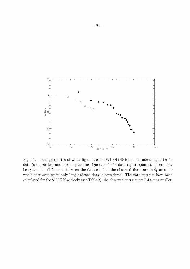
In Figure 11, we plot the flare energy spectrum (Lacy et al. 1976) as the estimated

flare energy as a function of the cumulative frequency (ν). The long-cadence Quarters 10-14

appear shifted with respect to the Quarter 14 data, simply because the observed flare rate

was lower. (Indeed, there are no candidate flares in Quarter 10.) Additional monitoring is

needed to improve the frequency estimates and to check if the flare rate varies. Comparison

to well studied dMe flare stars (Lacy et al. 1976; Gershberg 2005) indicates the flare energy

spectrum is similar to that observed in flare stars but shifted downwards for W1906+40:

Flares are ∼ 10 − 100 times less energetic at a given frequency, or alternatively flares of a

given energy are less frequent on W1906+40 than on dMe flare stars. On the other hand,

the white light flare rate on W1906+40 is comparable to that of the Sun (Neidig & Cliver

1983; Gershberg 2005), despite the L dwarf’s much lower effective temperature and surface

area. The observed rate for flares with energy > 1031 ergs is 10−3 to 10−2.5 hr−1, or 1-2

per month. For comparison, the Berger et al. (2010) limit on Hα-only L dwarf flares is a

cumulative frequency of log ν((hr−1) . −1.4; those flares are too weak to be detected in the

broad Kepler filter.

5. Conclusion

Our initial monitoring of W1906+40 has revealed long-lived surface features and a well-

defined periodicity due to rotation. Despite its cool photosphere, this L1 dwarf maintains

an active and variable chromosphere, emits in the radio, and produces powerful flares that

rival white light flares in the Sun. A major limiting factor in the analysis of the periodic

component is our lack of knowledge of the spot-to-star flux ratio. During our Guest Observer

Cycle 4 program, we are monitoring W1906+40 with a number of ground-based telescopes

– 17 –

to search for changes correlated with Kepler data and to determine if the surface features

change on multi-year timescales. These observations may be able to reveal the nature of the

surface features, and whether they are hotter or cooler than the surrounding photosphere.

We are grateful to Martin Still for approving the Kepler observations and to the USNO

infrared parallax team for allowing us to use the preliminary parallax measurement. We

thank Gibor Basri and Peter Plavchan for helpful discussions of Kepler photometry, Kamen

Todorov and David Hogg for discussions of MCMC methods, and Mark Giampapa, Suzanne

Hawley, Adam Kowalski, Dermott Mullan, and Lucianne Walkowicz for discussions of stellar

flares.

This paper includes data collected by the Kepler mission. Funding for the Kepler mis-

sion is provided by the NASA Science Mission directorate. The material is based upon work

supported by NASA under award No. NNX13AC18G. EB acknowledges support from the

National Science Foundation through Grant AST-1008361. The National Radio Astronomy

Observatory is a facility of the National Science Foundation operated under cooperative

agreement by Associated Universities, Inc. Based on observations obtained at the Gemini

Observatory, which is operated by the Association of Universities for Research in Astronomy,

Inc., under a cooperative agreement with the NSF on behalf of the Gemini partnership: the

National Science Foundation (United States), the Science and Technology Facilities Council

(United Kingdom), the National Research Council (Canada), CONICYT (Chile), the Aus-

tralian Research Council (Australia), Ministerio da Ciencia, Tecnologia e Inovacao (Brazil)

and Ministerio de Ciencia, Tecnologıa e Innovacion Productiva (Argentina) Some of the data

presented herein were obtained at the W.M. Keck Observatory, which is operated as a scien-

tific partnership among the California Institute of Technology, the University of California

and the National Aeronautics and Space Administration. The Observatory was made possi-

ble by the generous financial support of the W.M. Keck Foundation. This publication makes

use of data products from the Wide-field Infrared Survey Explorer, which is a joint project

of the University of California, Los Angeles, and the Jet Propulsion Laboratory/California

Institute of Technology, funded by the National Aeronautics and Space Administration.

Some of the data presented in this paper were obtained from the Mikulski Archive for Space

Telescopes (MAST). STScI is operated by the Association of Universities for Research in

Astronomy, Inc., under NASA contract NAS5-26555. Support for MAST for non-HST data

is provided by the NASA Office of Space Science via grant NNX09AF08G and by other

grants and contracts.

Facilities: Gemini:Gillett, Keck:II, Kepler, USNO:61in, VLA

– 18 –

REFERENCES

Alekseev, I. Y., & Gershberg, R. E. 1996, in Astronomical Society of the Pacific Conference

Series, Vol. 109, Cool Stars, Stellar Systems, and the Sun, ed. R. Pallavicini & A. K.

Dupree, 583

Allard, F., Homeier, D., & Freytag, B. 2011, in Astronomical Society of the Pacific Confer-

ence Series, Vol. 448, 16th Cambridge Workshop on Cool Stars, Stellar Systems, and

the Sun, ed. C. Johns-Krull, M. K. Browning, & A. A. West, 91

Allred, J. C., Hawley, S. L., Abbett, W. P., & Carlsson, M. 2006, ApJ, 644, 484

Artigau, E., Bouchard, S., Doyon, R., & Lafreniere, D. 2009, ApJ, 701, 1534

Bailer-Jones, C. A. L. 2004, A&A, 419, 703

Bailer-Jones, C. A. L., & Mundt, R. 1999, A&A, 348, 800

—. 2001, A&A, 367, 218

Basri, G., Walkowicz, L. M., Batalha, N., Gilliland, R. L., Jenkins, J., Borucki, W. J., Koch,

D., Caldwell, D., Dupree, A. K., Latham, D. W., Marcy, G. W., Meibom, S., &

Brown, T. 2011, AJ, 141, 20

Berger, E. 2002, ApJ, 572, 503

—. 2006, ApJ, 648, 629

Berger, E., Basri, G., Fleming, T. A., Giampapa, M. S., Gizis, J. E., Liebert, J., Martın, E.,

Phan-Bao, N., & Rutledge, R. E. 2010, ApJ, 709, 332

Berger, E., Basri, G., Gizis, J. E., Giampapa, M. S., Rutledge, R. E., Liebert, J., Martın,

E., Fleming, T. A., Johns-Krull, C. M., Phan-Bao, N., & Sherry, W. H. 2008a, ApJ,

676, 1307

Berger, E., Gizis, J. E., Giampapa, M. S., Rutledge, R. E., Liebert, J., Martın, E., Basri,

G., Fleming, T. A., Johns-Krull, C. M., Phan-Bao, N., & Sherry, W. H. 2008b, ApJ,

673, 1080

Berger, E., Rutledge, R. E., Phan-Bao, N., Basri, G., Giampapa, M. S., Gizis, J. E., Liebert,

J., Martın, E., & Fleming, T. A. 2009, ApJ, 695, 310

– 19 –

Berger, E., Rutledge, R. E., Reid, I. N., Bildsten, L., Gizis, J. E., Liebert, J., Martın, E.,

Basri, G., Jayawardhana, R., Brandeker, A., Fleming, T. A., Johns-Krull, C. M.,

Giampapa, M. S., Hawley, S. L., & Schmitt, J. H. M. M. 2005, ApJ, 627, 960

Blake, C. H., Charbonneau, D., & White, R. J. 2010, ApJ, 723, 684

Blake, C. H., Charbonneau, D., White, R. J., Torres, G., Marley, M. S., & Saumon, D. 2008,

ApJ, 678, L125

Buenzli, E., Apai, D., Morley, C. V., Flateau, D., Showman, A. P., Burrows, A., Marley,

M. S., Lewis, N. K., & Reid, I. N. 2012, ArXiv e-prints

Burgasser, A. J., Cruz, K. L., Cushing, M., Gelino, C. R., Looper, D. L., Faherty, J. K.,

Kirkpatrick, J. D., & Reid, I. N. 2010, ApJ, 710, 1142

Burgasser, A. J., Luk, C., Dhital, S., Bardalez Gagliuffi, D., Nicholls, C. P., Prato, L., West,

A. A., & Lepine, S. 2012, ArXiv e-prints

Burgasser, A. J., Melis, C., Zauderer, B. A., & Berger, E. 2013, ApJ, 762, L3

Burrows, A., Heng, K., & Nampaisarn, T. 2011, ApJ, 736, 47

Caballero, J. A., Bejar, V. J. S., Rebolo, R., & Zapatero Osorio, M. R. 2004, A&A, 424, 857

Caldwell, D. A., Kolodziejczak, J. J., Van Cleve, J. E., Jenkins, J. M., Gazis, P. R., Ar-

gabright, V. S., Bachtell, E. E., Dunham, E. W., Geary, J. C., Gilliland, R. L.,

Chandrasekaran, H., Li, J., Tenenbaum, P., Wu, H., Borucki, W. J., Bryson, S. T.,

Dotson, J. L., Haas, M. R., & Koch, D. G. 2010, ApJ, 713, L92

Chabrier, G., & Baraffe, I. 2000, ARA&A, 38, 337

Chabrier, G., Baraffe, I., Allard, F., & Hauschildt, P. 2000, ApJ, 542, 464

Claret, A. 1998, A&A, 335, 647

Claret, A., & Bloemen, S. 2011, A&A, 529, A75

Clarke, F. J., Oppenheimer, B. R., & Tinney, C. G. 2002, MNRAS, 335, 1158

Clarke, F. J., Tinney, C. G., & Hodgkin, S. T. 2003, MNRAS, 341, 239

Cram, L. E., & Woods, D. T. 1982, ApJ, 257, 269

Cruz, K. L., Kirkpatrick, J. D., & Burgasser, A. J. 2009, AJ, 137, 3345

– 20 –

Dorren, J. D. 1987, ApJ, 320, 756

Eason, E. L. E., Giampapa, M. S., Radick, R. R., Worden, S. P., & Hege, E. K. 1992, AJ,

104, 1161

Faherty, J. K., Burgasser, A. J., Cruz, K. L., Shara, M. M., Walter, F. M., & Gelino, C. R.

2009, AJ, 137, 1

Fischer, J., Vrba, F. J., Toomey, D. W., Lucke, B. L., Wang, S.-i., Henden, A. A., Robichaud,

J. L., Onaka, P. M., Hicks, B., Harris, F. H., Stahlberger, W. E., Kosakowski, K. E.,

Dudley, C. C., & Johnston, K. J. 2003, in Society of Photo-Optical Instrumentation

Engineers (SPIE) Conference Series, Vol. 4841, Society of Photo-Optical Instrumen-

tation Engineers (SPIE) Conference Series, ed. M. Iye & A. F. M. Moorwood, 564–577

Ford, E. B. 2005, AJ, 129, 1706

Fuhrmeister, B., Liefke, C., Schmitt, J. H. M. M., & Reiners, A. 2008, A&A, 487, 293

Fuhrmeister, B., Schmitt, J. H. M. M., & Hauschildt, P. H. 2010, A&A, 511, A83

Gelino, C., & Marley, M. 2000, in Astronomical Society of the Pacific Conference Series,

Vol. 212, From Giant Planets to Cool Stars, ed. C. A. Griffith & M. S. Marley, 322

Gelino, C. R., Marley, M. S., Holtzman, J. A., Ackerman, A. S., & Lodders, K. 2002, ApJ,

577, 433

Gershberg, R. E. 2005, Solar-Type Activity in Main-Sequence Stars (Springer)

Gilliland, R. L., Jenkins, J. M., Borucki, W. J., Bryson, S. T., Caldwell, D. A., Clarke, B. D.,

Dotson, J. L., Haas, M. R., Hall, J., Klaus, T., Koch, D., McCauliff, S., Quintana,

E. V., Twicken, J. D., & van Cleve, J. E. 2010, ApJ, 713, L160

Gizis, J. E., Monet, D. G., Reid, I. N., Kirkpatrick, J. D., Liebert, J., & Williams, R. J.

2000, AJ, 120, 1085

Gizis, J. E., Troup, N. W., & Burgasser, A. J. 2011, ApJ, 736, L34+

Golimowski, D. A., Leggett, S. K., Marley, M. S., Fan, X., Geballe, T. R., Knapp, G. R.,

Vrba, F. J., Henden, A. A., Luginbuhl, C. B., Guetter, H. H., Munn, J. A., Canzian,

B., Zheng, W., Tsvetanov, Z. I., Chiu, K., Glazebrook, K., Hoversten, E. A., Schnei-

der, D. P., & Brinkmann, J. 2004, AJ, 127, 3516

Gray, D. F. 1992, The observation and analysis of stellar photospheres. (Cambridge Univer-

sity Press)

– 21 –

Hallinan, G., Antonova, A., Doyle, J. G., Bourke, S., Brisken, W. F., & Golden, A. 2006,

ApJ, 653, 690

Hallinan, G., Antonova, A., Doyle, J. G., Bourke, S., Lane, C., & Golden, A. 2008, ApJ,

684, 644

Harding, L. K., Hallinan, G., Boyle, R. P., Butler, R. F., Sheehan, B., & Golden, A. 2011,

in Astronomical Society of the Pacific Conference Series, Vol. 448, 16th Cambridge

Workshop on Cool Stars, Stellar Systems, and the Sun, ed. C. Johns-Krull, M. K.

Browning, & A. A. West, 219

Hawley, S. L., & Fisher, G. H. 1992, ApJS, 78, 565

Hawley, S. L., & Pettersen, B. R. 1991, ApJ, 378, 725

Hilton, E. J., West, A. A., Hawley, S. L., & Kowalski, A. F. 2010, AJ, 140, 1402

Hook, I. M., Jørgensen, I., Allington-Smith, J. R., Davies, R. L., Metcalfe, N., Murowinski,

R. G., & Crampton, D. 2004, PASP, 116, 425

Houdebine, E. R. 1992, Irish Astronomical Journal, 20, 213

Hussain, G. A. J. 2002, Astronomische Nachrichten, 323, 349

Jenkins, J. M., Caldwell, D. A., Chandrasekaran, H., Twicken, J. D., Bryson, S. T., Quin-

tana, E. V., Clarke, B. D., Li, J., Allen, C., Tenenbaum, P., Wu, H., Klaus, T. C.,

Middour, C. K., Cote, M. T., McCauliff, S., Girouard, F. R., Gunter, J. P., Wohler,

B., Sommers, J., Hall, J. R., Uddin, A. K., Wu, M. S., Bhavsar, P. A., Van Cleve, J.,

Pletcher, D. L., Dotson, J. A., Haas, M. R., Gilliland, R. L., Koch, D. G., & Borucki,

W. J. 2010a, ApJ, 713, L87

Jenkins, J. M., Caldwell, D. A., Chandrasekaran, H., Twicken, J. D., Bryson, S. T., Quin-

tana, E. V., Clarke, B. D., Li, J., Allen, C., Tenenbaum, P., Wu, H., Klaus, T. C.,

Van Cleve, J., Dotson, J. A., Haas, M. R., Gilliland, R. L., Koch, D. G., & Borucki,

W. J. 2010b, ApJ, 713, L120

Kirkpatrick, J. D. 2005, ARA&A, 43, 195

Kirkpatrick, J. D., Reid, I. N., Liebert, J., Cutri, R. M., Nelson, B., Beichman, C. A., Dahn,

C. C., Monet, D. G., Gizis, J. E., & Skrutskie, M. F. 1999, ApJ, 519, 802

– 22 –

Koch, D. G., Borucki, W. J., Basri, G., Batalha, N. M., Brown, T. M., Caldwell, D.,

Christensen-Dalsgaard, J., Cochran, W. D., DeVore, E., Dunham, E. W., Gautier,

T. N., Geary, J. C., Gilliland, R. L., Gould, A., Jenkins, J., Kondo, Y., Latham,

D. W., Lissauer, J. J., Marcy, G., Monet, D., Sasselov, D., Boss, A., Brownlee, D.,

Caldwell, J., Dupree, A. K., Howell, S. B., Kjeldsen, H., Meibom, S., Morrison, D.,

Owen, T., Reitsema, H., Tarter, J., Bryson, S. T., Dotson, J. L., Gazis, P., Haas,

M. R., Kolodziejczak, J., Rowe, J. F., Van Cleve, J. E., Allen, C., Chandrasekaran,

H., Clarke, B. D., Li, J., Quintana, E. V., Tenenbaum, P., Twicken, J. D., & Wu, H.

2010, ApJ, 713, L79

Koen, C. 2003, MNRAS, 346, 473

—. 2005, MNRAS, 360, 1132

—. 2006, MNRAS, 367, 1735

Kowalski, A. F., Hawley, S. L., Holtzman, J. A., Wisniewski, J. P., & Hilton, E. J. 2010,

ApJ, 714, L98

Kowalski, A. F., Hawley, S. L., Holtzman, J. A., Wisniewski, J. P., & Hilton, E. J. 2011, in

IAU Symposium, Vol. 273, IAU Symposium, 261–264

—. 2012, Sol. Phys., 277, 21

Kruse, E. A., Berger, E., Knapp, G. R., Laskar, T., Gunn, J. E., Loomis, C. P., Lupton,

R. H., & Schlegel, D. J. 2010, ApJ, 722, 1352

Lacy, C. H., Moffett, T. J., & Evans, D. S. 1976, ApJS, 30, 85

Lane, C., Hallinan, G., Zavala, R. T., Butler, R. F., Boyle, R. P., Bourke, S., Antonova, A.,

Doyle, J. G., Vrba, F. J., & Golden, A. 2007, ApJ, 668, L163

Liebert, J., Kirkpatrick, J. D., Cruz, K. L., Reid, I. N., Burgasser, A., Tinney, C. G., &

Gizis, J. E. 2003, AJ, 125, 343

Liebert, J., Kirkpatrick, J. D., Reid, I. N., & Fisher, M. D. 1999, ApJ, 519, 345

Livingston, W., & Wallace, L. 1991, An atlas of the solar spectrum in the infrared from 1850

to 9000 cm-1 (1.1 to 5.4 micrometer) (National Solar Observatory)

Maehara, H., Shibayama, T., Notsu, S., Notsu, Y., Nagao, T., Kusaba, S., Honda, S.,

Nogami, D., & Shibata, K. 2012, Nature, 485, 478

Martın, E. L., & Ardila, D. R. 2001, AJ, 121, 2758

– 23 –

Martın, E. L., Delfosse, X., Basri, G., Goldman, B., Forveille, T., & Zapatero Osorio, M. R.

1999, AJ, 118, 2466

McLean, M., Berger, E., Irwin, J., Forbrich, J., & Reiners, A. 2011, ApJ, 741, 27

McLean, M., Berger, E., & Reiners, A. 2012, ApJ, 746, 23

McMullin, J. P., Waters, B., Schiebel, D., Young, W., & Golap, K. 2007, in Astronomical So-

ciety of the Pacific Conference Series, Vol. 376, Astronomical Data Analysis Software

and Systems XVI, ed. R. A. Shaw, F. Hill, & D. J. Bell, 127

Mohanty, S., Basri, G., Shu, F., Allard, F., & Chabrier, G. 2002, ApJ, 571, 469

Neidig, D. F., & Cliver, E. W. 1983, Sol. Phys., 88, 275

Radigan, J., Jayawardhana, R., Lafreniere, D., Artigau, E., Marley, M., & Saumon, D. 2012,

ApJ, 750, 105

Reid, I. N., Kirkpatrick, J. D., Gizis, J. E., Dahn, C. C., Monet, D. G., Williams, R. J.,

Liebert, J., & Burgasser, A. J. 2000, AJ, 119, 369

Reiners, A., & Basri, G. 2008, ApJ, 684, 1390

Rockenfeller, B., Bailer-Jones, C. A. L., Mundt, R., & Ibrahimov, M. A. 2006, MNRAS, 367,

407

Sault, R. J., & Wieringa, M. H. 1994, A&AS, 108, 585

Schmidt, S. J., Cruz, K. L., Bongiorno, B. J., Liebert, J., & Reid, I. N. 2007, AJ, 133, 2258

Stelzer, B., Schmitt, J. H. M. M., Micela, G., & Liefke, C. 2006, A&A, 460, L35

Stumpe, M. C., Smith, J. C., Van Cleve, J. E., Twicken, J. D., Barclay, T. S., Fanelli, M. N.,

Girouard, F. R., Jenkins, J. M., Kolodziejczak, J. J., McCauliff, S. D., & Morris, R. L.

2012, PASP, 124, 985

Vrba, F. J., Henden, A. A., Luginbuhl, C. B., Guetter, H. H., Munn, J. A., Canzian, B.,

Burgasser, A. J., Kirkpatrick, J. D., Fan, X., Geballe, T. R., Golimowski, D. A.,

Knapp, G. R., Leggett, S. K., Schneider, D. P., & Brinkmann, J. 2004, AJ, 127, 2948

Walkowicz, L. M., Basri, G., Batalha, N., Gilliland, R. L., Jenkins, J., Borucki, W. J., Koch,

D., Caldwell, D., Dupree, A. K., Latham, D. W., Meibom, S., Howell, S., Brown,

T. M., & Bryson, S. 2011, AJ, 141, 50

– 24 –

Williams, P. K. G., Berger, E., & Zauderer, B. A. 2013, ArXiv e-prints

Wright, E. L., Eisenhardt, P. R. M., Mainzer, A. K., Ressler, M. E., Cutri, R. M., Jarrett,

T., Kirkpatrick, J. D., Padgett, D., McMillan, R. S., Skrutskie, M., Stanford, S. A.,

Cohen, M., Walker, R. G., Mather, J. C., Leisawitz, D., Gautier, T. N., McLean, I.,

Benford, D., Lonsdale, C. J., Blain, A., Mendez, B., Irace, W. R., Duval, V., Liu,

F., Royer, D., Heinrichsen, I., Howard, J., Shannon, M., Kendall, M., Walsh, A. L.,

Larsen, M., Cardon, J. G., Schick, S., Schwalm, M., Abid, M., Fabinsky, B., Naes,

L., & Tsai, C. 2010, AJ, 140, 1868

Zirin, H. 1988, Astrophysics of the sun (Cambridge University Press)

Zirin, H., & Tanaka, K. 1973, Sol. Phys., 32, 173

This preprint was prepared with the AAS LATEX macros v5.2.

– 25 –

Table 1. WISEP J190648.47+401106.8

Parameter W1906+4011 Units

Sp. Type L1 optical

Sp. Type L1 near-infrareda

i 17.419± 0.006 mag a

Ks 11.77± 0.02 mag a

πabs 61.15± 1.30 mas

µ 476.2± 2.9 mas yr−1

θ 111.28± 0.17 degrees

vtan 36.9± 0.8 km s−1

vrad −22.6± 0.4 km s−1

U -5.5 km s−1 b

V -11.6 km s−1

W -41.3 km s−1

v sin i 11.2± 2.2 km s−1

Period 0.37015 days

Amplitude 1.5%

logLbol/L⊙ −3.67± 0.03

R 0.92± 0.07 RJ

sin i > 0.59

Radio νLν (4.5± 0.9)× 1022 erg s−1)

Radio α −2.0± 1.4

〈Hα EW〉 4 A

〈FHα〉 3× 10−16 erg s−1cm−2

log 〈FHα〉/Lbol -5.0

log νLν/Lbol -7.3

aFrom Gizis et al. (2011)

bU is positive towards Galactic center

– 26 –

Table 2. W1906+40 Kepler Calibration

Spectrum Count Rate L (4370-8360 A) Lbol

cnts s−1 1028 erg s−1 1028 erg s−1

L1 photosphere (W1906+40) 1 1.4 82

Flare (6000K Blackbody) 1 2.0 4.4

Flare (8000K Blackbody) 1 2.1 5.0

Flare (10000K Blackbody) 1 2.1 6.4

Flare (Scaled AD Leo Impulsive)a 1 2.1 6.8

Flare (Scaled AD Leo Gradual)a 1 2.1 5.2

aBased on Hawley & Pettersen (1991). See text

Table 3. Sample Single Circular Dark Spot Models

Parameter i = 50◦ i = 60◦ i = 70◦ i = 80◦

sin i 0.77 0.87 0.94 0.98

Median Observed Flux 1.000 1.000 1.000 1.000

Unspotted Flux 1.012 1.012 1.011 1.011

Latitude (deg) 73 77 81 83

Spot Radius (deg) 8.0 9.9 13 20

– 27 –

Table 4. Flares Observed in Quarter 14

Mission Time Peak Etot tL tr t1/2 PeakLC Notes

days cnts s−1 1030 erg s−1 min min min cnts s−1

1304.9353 4.27 160 106 7 5 1.35 Gemini spectra

1298.5401 1.34 48 160 23 22 1.16

1336.1666 2.42 40 37 3 2 1.17 Ended by 1336.1939

1348.8632 2.09 38 75 5 3 1.10

1358.5103 1.56 27 76 9 3 1.08

1336.1939 1.39 26 64 4 17 1.08

1302.2680 3.39 17 106 2 2 1.02

1304.8597 1.27 8.4 60 3 1 1.04 Gemini spectra, precedes 1304.9353

1287.6311 1.46 7.2 26 2 1 1.04

1340.6865 1.34 6.6 18 1 3 1.02

1362.5329 1.41 4.5 12 2 1 1.01

1357.3020 1.29 4.2 19 2 1 1.00

1299.4556 1.42 4.2 8 1 2 1.01

1352.5146 1.33 3.3 9 2 1 1.00

1286.4391 1.18 2.5 12 2 3 1.00

1314.9410 1.34 1.8 2 2 1 1.00

1288.1638 1.11 1.4 10 2 1 1.01

1331.0249 1.12 0.9 4 1 2 1.00

1366.0617 1.11 0.6 2 1 1 1.00

1323.4271 1.12 0.6 3 2 1 1.00

1318.0816 1.12 0.6 3 2 1 1.00

– 28 –

Phase

Rel

ativ

e B

right

ness

0.96

0.97

0.98

0.99

1.00

1.01

1.02

Q10

Q11

0.96

0.97

0.98

0.99

1.00

1.01

1.02

Q12

Q13

0.0 0.2 0.4 0.6 0.8 1.00.96

0.97

0.98

0.99

1.00

1.01

1.02

Q14

Fig. 1.— Phased Kepler light curves for W1906+40 for Quarters 10-14 for a period of

0.370152 days. Phase zero is defined as Kepler Mission day 1000.0. The red curve shows

a sine function with P = 0.370152 days and amplitude 0.00763. The light curve shows

significant differences in Quarter 13, but overall the light curve has a consistent phase and

amplitude.

– 29 –

1146 1147 1148 1149 1150Mission Time (days)

0.98

1.00

1.02

1.04

1.06

1.08

1.10

1.12

Rel

ativ

e K

eple

r B

right

ness

1146 1147 1148 1149 1150Mission Time (days)

0.98

1.00

1.02

1.04

1.06

1.08

1.10

1.12

Rel

ativ

e K

eple

r B

right

ness

1.48

Fig. 2.— Kepler light curve showing the Quarter 12 data from Mission Day 1146 to 1150.

The plotted error bars are those reported by the Kepler pipeline (0.044 for these points),

which may be underestimated. The red curve shows the model sine fit for the full year-long

dataset. Possible changes in the amplitude are evident, perhaps up to twice the model. The

time of the radio observations (Section 2.3) is marked by the vertical blue line with one hour

before and after shown as the dotted line. The flare candidate at 1148.41 is discussed in

Section 4.2.

– 30 –

4000 6000 8000 10000Wavelength (Angstroms)

0.0

0.2

0.4

0.6

0.8

Cou

nts

per

seco

nd p

er A

ngst

rom

Counts due to L1 Dwarf Photosphere

Kepler Filter Curve

with 8000K Flare

Fig. 3.— Predicted count rates as a function of wavelength for the Kepler photometer. We

use the L1 standard 2MASS J14392836+1929149 (Kirkpatrick et al. 1999) for λ > 6300 Aand

the L0.5 dwarf 2MASS J07464256+2000321 (Reid et al. 2000) for λ ≤ 6300A in order to

completely cover the Kepler filter sensitivity range. The counts are weighted by the average

Kepler filter response (Koch et al. 2010), which is also plotted by itself. The integrated count

rate is normalized to give 660 electrons per second, which matches the pipeline reported count

rate for Quarter 10. Also shown is a hypothetical 8,000K blackbody flare (Walkowicz et al.

2011) that contributes an equal number of counts.

– 31 –

6500 7000 7500 8000 8500Wavelength (Angstroms)

0

2•10-16

4•10-16

6•10-16

8•10-16

f λ (

erg

s-1 c

m-2

Ang

stro

ms-1

)

W1906+40 quiscent

W1906+40 flare UT 10:14

Hα

HeI

HeI

HeI

OI

Fig. 4.— Gemini spectrum of W1906+40 (without telluric correction) in a quiescent, appar-

ently non-flaring, period and in a white light flare. The spectral type is L1 on the Kirkpatrick

et al. (1999) system.

100 200 300 400 500 600Pixels

0.0

0.5

1.0

1.5

2.0

Nor

mal

ized

Flu

x

2.29223 2.29595 2.29954 2.30303 2.30643 2.30973 2.31295Wavelength (µm)

O-C

W1906+40112300/5.0/-22.5/11.0

χ2r = 2.92940

Fig. 5.— Keck II NIRSPEC spectrum of W1906+40 with best-fit model to the data.

– 32 –

Pro

babi

lity

0.6 0.8 1.0 1.2Radius (RJ)

0.00

0.02

0.04

0.06

0.08

0.10

0.12

0.14

0.0 0.2 0.4 0.6 0.8 1.0sin i

Fig. 6.— Posterior Probability Distribution for the radius and inclination (sin i) of

W1906+40 given the constraints of the observed luminosity, effective temperature, period,

and v sin i.

Wavelength (Angstroms)

f λ (

10-1

7 erg

s-1

cm

-2 A

ngst

rom

s-1)

10

100

1000UT 10:14:15

10

100

1000UT 10:31:27

6400 6600 6800 7000 7200 7400

10

100

1000UT 10:41:56

Fig. 7.— The first three observed spectra during the main flare on 29 July 2012, with the

L dwarf photosphere (Figure 4) subtracted off. Note the strong white light continuum, the

broad H α that narrows, and the helium emission lines. The first spectrum has been adjusted

upwards by a factor of 1.67 based on the timing of the flare in the Kepler photometry.

– 33 –

Time (days)

Flu

x (1

0-16 e

rg s

-1 c

m-2)

0

5.0•103

1.0•104

1.5•104

2.0•104

2.5•104

Kepler White Light

0

100

200

300

400

H alpha

1304.85 1304.90 1304.95 1305.00 1305.0502

4

6

8

10

12

14He I

O I

Fig. 8.— Kepler white light and Gemini emission line flux as a function of time. The early,

main, and later flares are evident. The line fluxes measured with Gemini at the start of

the two flares (1304.86 and 1304.93) have been adjusted upwards based on the timing of

the flare start times in the Kepler photometry. The Kepler white light flux is calculated for

the wavelength range 4370-8360 A; the ultraviolet plus optical flux is probably two to three

times higher (Table 2).

Time from Peak (days)

Rel

ativ

e B

right

ness

(cn

ts/s

ec)

1.01.52.02.53.03.5

1302.2680

1336.1666

1.0

1.5

2.0

2.5

3.0 1348.8632

1358.5103

1.01.21.41.61.82.0

1287.6311

1362.5329

1.01.21.41.61.82.0

1299.4556

1336.1939

-0.010 -0.005 0.000 0.005 0.010 0.015 0.0201.01.21.41.61.82.0

1298.5401

-0.010 -0.005 0.000 0.005 0.010 0.015 0.020

1314.9410

Fig. 9.— Quarter 14 Kepler photometry of white light flares. Note the different scales for

the upper plots.

– 34 –

Time (days)

Rel

ativ

e B

right

ness

0.91.01.11.21.31.41.5

1017.8398

1139.1095

0.91.01.11.21.31.41.5

1148.4069

1206.0315

-0.2 0.0 0.2 0.40.91.01.11.21.31.41.5

1213.6127

-0.2 0.0 0.2 0.4

1266.3336

Fig. 10.— Quarters 11-13 long cadence photometry of candidate white light flares. Not

shown is another flare at time 1039.04 where W1906+40 doubles in brightness, but is flagged

as possible cosmic ray. See discussion in the text. There are no flare candidates in Quarter

10.

– 35 –

-4.0 -3.5 -3.0 -2.5 -2.0 -1.529

30

31

32

33

log

E (

erg)

log ν (hr−1)

Fig. 11.— Energy spectra of white light flares on W1906+40 for short cadence Quarter 14

data (solid circles) and the long cadence Quarters 10-13 data (open squares). There may

be systematic differences between the datasets, but the observed flare rate in Quarter 14

was higher even when only long cadence data is considered. The flare energies have been

calculated for the 8000K blackbody (see Table 2); the observed energies are 2.4 times smaller.