kekb accelerator commissioning of kekbptep 2013, 03a010 t. abe et al. table 1. machine parameters...

Prog. Theor. Exp. Phys. 2013, 03A010 (25 pages)DOI: 10.1093/ptep/pts101

KEKB Accelerator

Commissioning of KEKB

Tetsuo Abe1, Kazunori Akai1, Yunhai Cai2, Kiyokazu Ebihara1, Kazumi Egawa1,Atsushi Enomoto1, John Flanagan1, Hitoshi Fukuma1, Yoshihiro Funakoshi1,∗,Kazuro Furukawa1, Takaaki Furuya1, Junji Haba1, Shigenori Hiramatsu1,Kenji Hosoyama1, Takao Ieiri1, Naoko Iida1, Hitomi Ikeda1, Masako Iwasaki1,Tatsuya Kageyama1, Susumu Kamada1, Takuya Kamitani1, Shigeki Kato1,Mitsuo Kikuchi1, Eiji Kikutani1, Haruyo Koiso1, Shin-ichi Kurokawa1, Mika Masuzawa1,Toshihiro Matsumoto1, Toshihiro Mimashi1, Takako Miura1, Akio Morita1,Yoshiyuki Morita1, Tatsuro T. Nakamura1, Kota Nakanishi1, Michiru Nishiwaki1,Yujiro Ogawa1, Kazuhito Ohmi1, Yukiyoshi Ohnishi1, Satoshi Ohsawa1, Norihito Ohuchi1,Katsunobu Oide1, Toshiyuki Oki1, Masaaki Ono1, Eugene Perevedentsev3, Kotaro Satoh1,Masanori Satoh1, Yuji Seimiya1, Kyo Shibata1, Miho Shimada1, Masaaki Suetake1,Yusuke Suetsugu1, Takashi Sugimura1, Tsuyoshi Suwada1, Osamu Tajima1,Masafumi Tawada1, Masaki Tejima1, Makoto Tobiyama1, Noboru Tokuda1,Sadaharu Uehara1, Shoji Uno1, Yasuchika Yamamoto1, Yoshiharu Yano1,Kazue Yokoyama1, Masato Yoshida1, Mitsuhiro Yoshida1, Shin-ichi Yoshimoto1,Masakazu Yoshioka1, Demin Zhou1, and Zhanguo Zong1

1KEK, High Energy Accelerator Organization, Oho 1-1, Tsukuba, Ibaraki 305-0801, Japan2SLAC National Accelerator Laboratory, Stanford University, Menlo Park, CA 94025, USA3The Budker Institute of Nuclear Physics, Academician Lavrentyev 11, 630090 Novosibirsk, Russia∗E-mail: [email protected]

Received October 10, 2012; Accepted December 25, 2012; Published March 25, 2013

. . . . . . . . . . . . . . . . . . . . . . . . . . . . . . . . . . . . . . . . . . . . . . . . . . . . . . . . . . . . . . . . . . . . . . . . . . . . . . .The machine commissioning of KEKB started in December 1998 and its operation was termi-nated at the end of June 2010 to upgrade KEKB to SuperKEKB. In this paper, we describe thecommissioning procedure of KEKB from 2002 to 2010.. . . . . . . . . . . . . . . . . . . . . . . . . . . . . . . . . . . . . . . . . . . . . . . . . . . . . . . . . . . . . . . . . . . . . . . . . . . . . . .

1. Introduction

KEKB [1] is an energy-asymmetric double-ring collider for B meson physics. Its operation startedin December 1998 and finished at the end of June 2010. During these ten-and-a-half years, KEKBachieved the world’s highest luminosity in both the peak and integrated luminosities. KEKB consistsof an 8 GeV electron ring (the high energy ring; HER), a 3.5 GeV positron ring (the low energy ring;LER) and their injector, which is a linac-complex providing the rings with both electron and positronbeams. The issues with the beam commissioning in the first four years have been described in aprevious paper [2]. In this paper, we describe the subsequent history of the beam commissioning.Emphasis is placed on how we have increased the luminosity and what issues remain unsolved.

© The Author(s) 2013. Published by Oxford University Press on behalf of the Physical Society of Japan.This is an Open Access article distributed under the terms of the Creative Commons Attribution License (http://creativecommons.org/licenses/by/3.0),which permits unrestricted use, distribution, and reproduction in any medium, provided the original work is properly cited.

at High E

nergy Accelerator R

esearch Organization(K

EK

) on January 15, 2015http://ptep.oxfordjournals.org/

Dow

nloaded from

http://ptep.oxfordjournals.org/

PTEP 2013, 03A010 T. Abe et al.

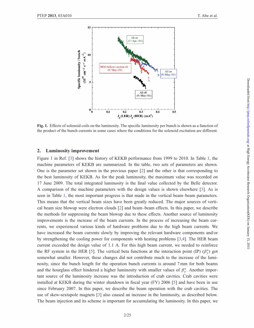
Fig. 1. Effects of solenoid coils on the luminosity. The specific luminosity per bunch is shown as a function ofthe product of the bunch currents in some cases where the conditions for the solenoid excitation are different.

2. Luminosity improvement

Figure 1 in Ref. [3] shows the history of KEKB performance from 1999 to 2010. In Table 1, themachine parameters of KEKB are summarized. In the table, two sets of parameters are shown.One is the parameter set shown in the previous paper [2] and the other is that corresponding tothe best luminosity of KEKB. As for the peak luminosity, the maximum value was recorded on17 June 2009. The total integrated luminosity is the final value collected by the Belle detector.A comparison of the machine parameters with the design values is shown elsewhere [3]. As isseen in Table 1, the most important progress is that made in the vertical beam–beam parameters.This means that the vertical beam sizes have been greatly reduced. The major sources of verti-cal beam size blowup were electron clouds [2] and beam–beam effects. In this paper, we describethe methods for suppressing the beam blowup due to these effects. Another source of luminosityimprovements is the increase of the beam currents. In the process of increasing the beam cur-rents, we experienced various kinds of hardware problems due to the high beam currents. Wehave increased the beam currents slowly by improving the relevant hardware components and/orby strengthening the cooling power for components with heating problems [3,4]. The HER beamcurrent exceeded the design value of 1.1 A. For this high beam current, we needed to reinforcethe RF system in the HER [5]. The vertical beta functions at the interaction point (IP) (β∗

y ) gotsomewhat smaller. However, these changes did not contribute much to the increase of the lumi-nosity, since the bunch length for the operation bunch currents is around 7 mm for both beamsand the hourglass effect hindered a higher luminosity with smaller values of β∗

y . Another impor-tant source of the luminosity increase was the introduction of crab cavities. Crab cavities wereinstalled at KEKB during the winter shutdown in fiscal year (FY) 2006 [5] and have been in usesince February 2007. In this paper, we describe the beam operation with the crab cavities. Theuse of skew-sextupole magnets [3] also caused an increase in the luminosity, as described below.The beam injection and its scheme is important for accumulating the luminosity. In this paper, we

2/25

at High E

nergy Accelerator R


EK


Dow

nloaded from



Table 1. Machine parameters of KEKB. Two sets of parameters are shown. One is the set of parametergiven in a previous paper [2] and the other is the set that corresponds to the best luminosity at KEKB.

up to 31 May 2010 up to 31 Oct. 2001

LER HER LER HER

Circumference 3016 3016 mRF frequency 508.89 508.89 MHzHarmonic number 5120 5120Horizontal emittance 18 24 18 24 nmBeam current 1637 1188 1072 761 mANumber of bunches 1585 1153Bunch current 1.03 0.75 0.93 0.66 mABunch spacing 1.84 2.36 mTotal RF voltage 8.0 13.0 6.5 12.0 MVSynchrotron tune νs −0.0246 −0.0209 −0.0223 −0.0199Horizontal tune νx 45.506 44.511 45.51 44.52Vertical tune νy 43.561 41.585 43.57 41.59Beta values at IP β∗

x /β∗y 120/0.59 120/0.59 59/0.65 63/0.70 cm

Momentum compaction α 3.31 3.43 3.41 3.38 ×10−4

Beam–beam parameter ξx 0.127 0.102 0.073 0.061Beam–beam parameter ξy 0.129 0.090 0.047 0.035Beam lifetime 133@1637 200@1188 101@1072 266@761 min@mALuminosity (Belle CsI) 2.108 × 1034 0.517 × 1034 cm−2 s−1

Total integrated luminosity 1041 42 fb−1

describe the continuous injection scheme, which contributed greatly to the integrated luminosityat KEKB.

3. Effects of electron clouds

In the history of KEKB, vertical beam size blowup due to electron clouds has been a very severeobstacle to obtaining a higher luminosity. The nature of the blowup has been studied theoretically andexperimentally [7,8]. In the beam operation, the effects of electron clouds were drastically suppressedby the installation of solenoid coils all around the LER ring [2]. The effects of the solenoid coilswere clearly observed in 2001, as shown in Fig. 1. In the figure, the specific luminosity per bunchis depicted as a function of the product of the bunch currents of the two beams. Here, the specificluminosity per bunch is defined as the total luminosity/(the number of bunches × the product of thebunch currents). As seen in the figure, when we switched off all the solenoids, the specific luminositybecame almost half of that with the solenoids.

Figure 2 shows the history of the length of the region where the solenoids coils are installed. Thesolenoid coils were installed on several occasions and about 95% of the drift space of the LER ringwas covered with the solenoid field Bz > 20 G. Although the solenoids drastically improved theluminosity, we found that performance of KEKB was still affected by electron clouds when an LERbeam current higher than about 1.6 A was used. The luminosity of KEKB did not increase with anLER beam current higher than about 1.6 A. It is believed that this is due to the effects of electronclouds. For this reason, the operation beam current in the LER of 1.6 A is much lower than the designbeam current of 2.6 A. Another impact of the electron clouds on the beam operation at KEKB isthe choice of bunch spacing. In the design, the bunch spacing is one RF-bucket, which means thatevery RF-bucket is filled with beam particles. However, in the actual operation, the bunch spacing isapproximately 3 RF-buckets. With shorter bunch spacing, the specific luminosity was reduced. Thisrestriction on bunch spacing is also believed to come from the effects of the electron clouds.

3/25

at High E

nergy Accelerator R


EK


Dow

nloaded from



Fig. 2. Installation history of solenoid coils in the LER ring.

0 10 20 30 40 50Bunch ID (MOD[49])

0

.001

.002

.003

.004

.005

.006

Spec

ific

Lum

inos

ity [

arbi

trar

y]

Fig. 3. Specific luminosity per bunch depending on the bunch position in the unit 49 RF-buckets. Each datumis the average of 99 bunches in the equivalent position in the unit 49 RF-buckets and the error bars are thestandard deviations of the 99 bunches.

Figure 3 shows the result of an experiment on bunch spacing carried out on 21 March 2008. Forthe experiment, a special filling pattern was used. In the beam filling pattern of KEKB, the samepattern should be repeated every 49 RF-buckets to be compatible with two-bunch injection. Due tothe synchronization problem between the injector linac and the KEKB rings, only the two bunchesin 49 RF-buckets in the rings can be injected from the linac to the rings. In the filling pattern used inthe experiment, 17 RF-buckets out of 49 RF-buckets were filled with the beam and the same patternsrepeated 99 times. Most of the bunch spacing between adjacent bunches was 3 RF-buckets but only2 bunches out of 17 bunches in a unit of 49 RF-buckets followed the preceding bunches at a distanceof 2 RF-buckets. In Fig. 3, the specific luminosity per bunch is plotted as a function of bunch ID in aunit of 49 RF-buckets. Note that the specific luminosity of each bunch ID in the figure is the averageof 99 bunches in the equivalent position in the units of 49 RF-buckets. The error bars in the graph

4/25

at High E

nergy Accelerator R


EK


Dow

nloaded from



Table 2. Tuning knobs for the luminosity and their observables. Many depend only onthe beam size at the synchrotron radiation monitor (SRM), besides the luminosity.

Knob Observable Frequency

Beam offset at IP (orbit feedback) Beam–beam kick (BPMs) ∼1 sCrossing angle at IP (orbit feedback) BPMs ∼1 sTarget of orbit feedback at IP (offset) vertical size at SRM, luminosity ∼1/2 dayTarget of orbit feedback at IP (angle) vertical size at SRM, luminosity ∼1/2 dayGlobal closed orbit BPMs ∼20 sBetatron tunes tunes of non-colliding bunches ∼20 sRelative RF phase center of gravity of the vertex ∼10 minGlobal coupling, dispersion, beta-beat orbit response to kicks, RF freq. ∼14 daysVertical waist position vertical size at SRM, luminosity ∼1/2 dayx–y coupling and dispersion at IP vertical size at SRM, luminosity ∼1/2 dayChromaticity of x–y coupling at IP vertical size at SRM, luminosity ∼1/2 day

show the standard deviations of the 99 bunches. As is seen in the figure, the specific luminosity after2 RF-buckets is ∼15% lower than that of the other bunches. It is believed that this degradation in thespecific luminosity comes from the effects of the electron clouds. In the case of short bunch trains,this degradation was not observed; thus, we can disprove the possibility that the degradation in thespecific luminosity after short bunch spacing is caused by the effects of parasitic collisions.

4. Methods of luminosity tuning

There are a number of knobs for tuning the luminosity. Only a few of them can be tuned up withindependent observables besides the luminosity. Table 2 lists the tuning parameters and their observ-ables. Tuning parameters related to the crab cavities are not listed in the table. We found that the linearoptics correction is important for suppressing the beam–beam blowup. In the usual beam operation,we frequently (typically every 2 weeks) made optics corrections where we corrected global betafunctions, x–y coupling parameters, and dispersions [2]. Sometimes, the optics corrections weredone with a different set of sextupole magnet strengths to narrow the stop-band of the resonance(2νx + νs = integer) or (2νx + 2νs = integer). The optics correction is the basis of the luminositytuning. On this basis, we carried out tuning on the other parameters in Table 2. At KEKB, we foundthat the local x–y coupling and the vertical dispersion at the IP are very important for increasing theluminosity. We have developed tuning knobs to adjust these parameters. In the following, we describethese knobs. The parameters are changed by changing the beam orbits. Figures 4 and 5 show exam-ples of the orbit form for changing the parameters. In the case of the LER (Fig. 4), 8 orbit bumpsare made to control the x–y coupling and the vertical dispersion parameters. Each bump is createdat a pair of (defocusing) sextupole (SD) magnets. At KEKB, we use the non-interleaved sextupolescheme. Each bump is almost localized at the pair of SD magnets. Since a tail of the bump is slightlyextended to the position of SF magnets next to the SD magnets, their effects are counted correctlyin the calculation. The paired SD magnets are connected with pseudo −I transformers (−I ′). In thissituation, if we make a symmetric bump at the paired sextupole magnets, the vertical dispersion islocalized between them and the x–y coupling is leaked around the ring. On the other hand, in thecase of an asymmetric bump, the x–y coupling is localized and the dispersion is leaked. In a realoperation, 8 symmetric and/or asymmetric bumps are created to meet the condition that the x–ycoupling and the vertical dispersion are localized in the bump section and R1, R2, R3, R4, ηy (thevertical dispersion) at the IP and η′

y (the slope of the vertical dispersion) at the IP are equal to target

5/25

at High E

nergy Accelerator R


EK


Dow

nloaded from



ym

y(m

m)

y(m

m)

0 100 200 300 400-400 -300 -200 -100

0-.5-1

-1.5

1.5

.51

15

50

2520

10

0

50

-50

100

-100

LER IP Dispersion / Tilt

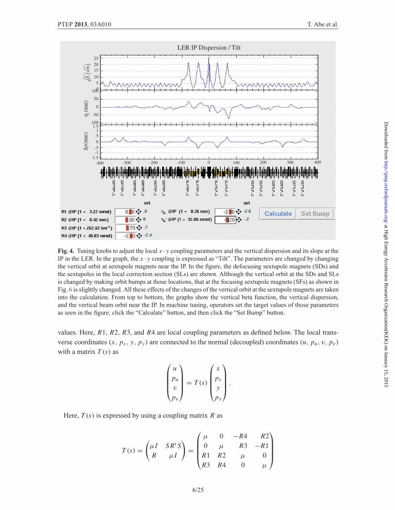
Fig. 4. Tuning knobs to adjust the local x–y coupling parameters and the vertical dispersion and its slope at theIP in the LER. In the graph, the x–y coupling is expressed as “Tilt”. The parameters are changed by changingthe vertical orbit at sextupole magnets near the IP. In the figure, the defocusing sextupole magnets (SDs) andthe sextupoles in the local correction section (SLs) are shown. Although the vertical orbit at the SDs and SLsis changed by making orbit bumps at those locations, that at the focusing sextupole magnets (SFs) as shown inFig. 6 is slightly changed. All these effects of the changes of the vertical orbit at the sextupole magnets are takeninto the calculation. From top to bottom, the graphs show the vertical beta function, the vertical dispersion,and the vertical beam orbit near the IP. In machine tuning, operators set the target values of those parametersas seen in the figure, click the “Calculate” button, and then click the “Set Bump” button.

values. Here, R1, R2, R3, and R4 are local coupling parameters as defined below. The local trans-verse coordinates (x, px , y, py) are connected to the normal (decoupled) coordinates (u, pu, v, pv)with a matrix T (s) as ⎛

⎜⎜⎜⎝upu

v

pv

⎞⎟⎟⎟⎠ = T (s)

⎛⎜⎜⎜⎝

xpx

ypy

⎞⎟⎟⎟⎠ .

Here, T (s) is expressed by using a coupling matrix R as

T (s) =(μI S Rt SR μI

)=

⎛⎜⎜⎜⎝μ 0 −R4 R20 μ R3 −R1

R1 R2 μ 0R3 R4 0 μ

⎞⎟⎟⎟⎠

6/25

at High E

nergy Accelerator R


EK


Dow

nloaded from



ym

y(m

m)

y(m

m)

0-.5-1

-1.5

1.5

.51

15

50

25 20

10

0

50

-50

100

-100

3035

0 200 400-400 -200

HER IP Dispersion / Tilt

Fig. 5. Tuning knobs to adjust the local x–y coupling parameters and the vertical dispersion and its slopeat the IP in the HER. In the graph, the x–y coupling is expressed as “Tilt”. The parameters are changed bychanging the vertical orbit at sextupole magnets near the IP. In the figure, the defocusing sextupole magnets(SDs) are shown.

and

S =(

0 1−1 0

), μ2 + detR = 1.

The locations of the sextupole magnets are shown in Figs. 4 and 5 together with typical shapes ofthe orbit bumps and some other optical parameters. As is seen in Fig. 4, the bump section is around±350 m of the IP (about 700 m in total) in the LER. In the figures, the center is the IP. KEKB has a200 m straight section around the IP. In the case of the LER, a local chromaticity correction schemeis installed in this straight section. Four SL magnets shown in Fig. 4 are sextupole magnets for thelocal correction. (We also use the non-interleaved sextupole scheme for the local correction.) Wealso make bumps at the paired sextupole magnets for the local correction. The HER case is almostthe same except that we have no local chromaticity correction for the HER and so the length of thebump section is somewhat longer compared with the LER case. We need a larger number of sex-tupole magnets in the arc section in the HER where we cannot use the sextupole magnets in the localchromaticity correction section as part of the knob. We have enough free parameters (16 parametersfor the height of the symmetric and asymmetric bumps) and so, in principle, it is possible to adjustthe coupling and dispersion parameters independently. As for the orbit itself, we can set the bumpswith sufficient accuracy, since the continuous closed orbit correction (CCC) system corrects the orbitif there is any deviation from the target orbit. However, machine errors may degrade the parameter

7/25

at High E

nergy Accelerator R


EK


Dow

nloaded from



180 200 220 240 260 280 300 3200

1

2

3

4

5

6-.4-.2

0.2.4.6.81

1.2

ym

x(m

)x

m

02468

101214

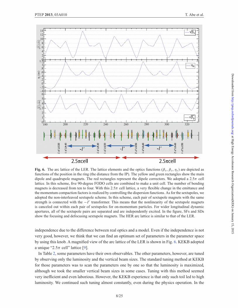
Fig. 6. The arc lattice of the LER. The lattice elements and the optics functions (βx , βy , ηx ) are depicted asfunctions of the position in the ring (the distance from the IP). The yellow and green rectangles show the maindipole and quadrupole magnets. The red rectangles represent the dipole correctors. We adopted a 2.5π celllattice. In this scheme, five 90-degree FODO cells are combined to make a unit cell. The number of bendingmagnets is decreased from ten to four. With this 2.5π cell lattice, a very flexible change in the emittance andthe momentum compaction factors is realized by controlling the dispersion functions. As for the sextupoles, weadopted the non-interleaved sextupole scheme. In this scheme, each pair of sextupole magnets with the samestrength is connected with the −I ′ transformer. This means that the nonlinearity of the sextupole magnetsis canceled out within each pair of sextupoles for on-momentum particles. For wider longitudinal dynamicapertures, all of the sextupole pairs are separated and are independently excited. In the figure, SFs and SDsshow the focusing and defocusing sextupole magnets. The HER arc lattice is similar to that of the LER.

independence due to the difference between real optics and a model. Even if the independence is notvery good, however, we think that we can find an optimum set of parameters in the parameter spaceby using this knob. A magnified view of the arc lattice of the LER is shown in Fig. 6. KEKB adopteda unique “2.5π cell” lattice [9].

In Table 2, some parameters have their own observables. The other parameters, however, are tunedby observing only the luminosity and the vertical beam sizes. The standard tuning method at KEKBfor those parameters was to scan the parameters one by one so that the luminosity is maximized,although we took the smaller vertical beam sizes in some cases. Tuning with this method seemedvery inefficient and even laborious. However, the KEKB experience is that only such toil led to highluminosity. We continued such tuning almost constantly, even during the physics operation. In the

8/25

at High E

nergy Accelerator R


EK


Dow

nloaded from



0 0.5 1.51 2Ib,LER (mA)

0

.02

.04

.06

.08

.12

.14

.1

y,H

ER

Fig. 7. Predicted beam–beam parameters by the strong–strong beam–beam simulations with a crossing angleof 22 mrad (purple) and the head-on collision (crab crossing) (red). Some experimental data are also shownwith squares. The black and green squares denote data with and without the crab cavities, respectively.

process of tuning with the crab cavities, we developed a tuning method in which 12 parameters aresearched at the same time, as is described in the next section.

5. Operation with crab cavities

5.1. Motivation for installing crab cavities

One of the design features of KEKB is the horizontal crossing angle of ±11 mrad at the IP. Althoughthere are many merits of the crossing angle scheme, the beam–beam performance may degrade. Thedesign of KEKB predicted that the vertical beam–beam parameter ξy could be as high as 0.05, ifbetatron tunes are properly chosen. The crab crossing scheme was proposed in 1988 by R. Palmer[10] as an idea to recover the head-on collision with the crossing angle for linear colliders. It hasalso been shown that the synchro–betatron coupling terms associated with the crossing angle in ringcolliders are canceled by crab crossing [11]. As discussed in Ref. [3], the development of the crabcavities at KEKB has been encouraged by beam-beam simulations [12–14], which predicted a veryhigh beam-beam parameter of ξy ∼ 0.15. Figure 7 shows a comparison between ξy for the head-oncollision (crab crossing) and the crossing angle by a strong–strong beam–beam simulation. After along R&D period, the crab cavities were finally installed at KEKB in February 2007.

5.2. Single crab cavity scheme

As explained in Ref. [3], we have developed the single crab cavity scheme. The layout is shown inFig. 2 in Ref. [3]. This scheme not only saved the cost of the cavities, but made it possible to usethe existing cryogenic system in the Nikko region, which has been utilized for the superconductingaccelerating cavities.

In the single crab cavity scheme, the following equation should be met for both beams to realize ahead-on collision:

φx

2=√βC

x β∗x cos(πνx − |ψC

x ])

2 sinπνx

VcωRF

Ec. (1)

9/25

at High E

nergy Accelerator R


EK


Dow

nloaded from



Table 3. Typical parameters for the crab cavities. The crossing angle,the horizontal beta functions at the IP and the crab cavities, the horizontaltunes, the horizontal phase advance from the cavities to the IP, the crabvoltage, and the RF frequency are shown.

LER HER

φx 22 mradβ∗

x 1.2 1.2 mβC

x 51 122 mνx 45.506 44.511ψC

x /2π 0.25 0.25Vc 0.97 1.45 MVfRF 508.89 MHz

Here, φx is the full crossing angle. βCx and β∗

x are the beta functions at the crab cavity and the IP,respectively.ψC

x denotes the horizontal betatron phase advance between the crab cavity and the IP.νx is the horizontal tune. Vc and ωRF are the crab voltage and the angular RF frequency (= 2π fR F),respectively. Typical values for these parameters are shown in Table 3.

The beam optics was modified for the crab cavities to provide the necessary magnitude of the betafunctions at the cavities and the proper phase advance between the cavities and the IP. A number ofquadrupoles have switched polarity and have started to have independent power supplies.

5.3. Tuning method of crab cavity parameters with beams and beam tuning with crabcavities

5.3.1. Crab voltage. Prior to the beam operation, calibration of the crab voltage was done by usingthe klystron output power and the loaded Q values of the crab cavities without actual beams. Thecrab voltage was also calibrated by using beams. If a bunch passes by the crab cavity at the zero-crosstiming of the crab RF voltage, the center of the bunch receives no dipole kick. When the crab phaseshifts from this condition, the bunch receives a net dipole kick from the cavity, like the case of asteering magnet. This dipole kick causes a closed orbit distortion (COD), the size of which dependson the crab phase. From the CODs around the ring created by the crab cavity, the dipole kick anglecan be estimated. By scanning the crab phase by more than 360◦ and fitting the kick angle estimatedat each data point as a function of the crab phase, the crab voltage can be determined. The crabvoltage thus determined is consistent with that calibrated from the klystron power and the Q valuewithin a few percent. From the crab phase scan and the fit, the phase shifter of the crab cavity systemcan also be calibrated. In the actual beam operation in the physics run mode, the crab voltages ofboth rings are scanned to maximize the luminosity, as is shown below.

5.3.2. Crab phase. In principle, the crab phase should be set so that the center of the bunch passesby at the zero-cross timing of the crab cavity. In this condition, the bunch receives no net dipole kick.This condition can be found by scanning the crab phase as described above. However, this methodis rather time-consuming and so an easier method is used in the usual operation. This method is tosearch for a crab phase that causes no change in the COD between the crab on and off by trial anderror. Although there are two zero-cross phases, we can choose the correct phase by observing thephase of the COD. In the actual physics run, in which high beam currents are needed, the crab phaseis shifted by some amount (typically 10◦) to suppress the dipole oscillation observed at high-currentcrab collision. The COD induced by the net dipole kick by the crab cavity can be compensated bysteering magnets in the ring.

10/25

at High E

nergy Accelerator R


EK


Dow

nloaded from



5.3.3. Beam orbits at the crab cavities. The beam loading for the crabbing mode increases linearlyas a function of a horizontal orbit displacement from the center of the crab cavity. If the RF powerto operate the cavity is too sensitive to the beam orbit, cavity operation under the existence of thebeams could be difficult. To avoid this situation, we have chosen the loaded Q value of the cavity tobe QL = (1 − 2)× 105. With this relatively low Q value, the RF power for the operation is relativelyhigh (typically 100 kW at 1.4 MV). However, the RF power becomes less sensitive to the beam orbit(typically 20% change for 1 mm orbit change). When we condition the cavity, we need a higherpower. However, with this Q value, 200 kW is sufficient for conditioning the cavity up to 2 MV. Inaddition, we have developed an orbit feedback system to keep the horizontal beam orbit at the crabcavity stable [16]. This system is composed of 4 horizontal steering magnets to make an offset bumpfor each ring and 4 beam position monitors (BPMs) for each ring to monitor the beam orbit at thecrab cavity. The design system speed is 1 Hz and the target accuracy of the orbit is within 0.1 mm.However, in the actual beam operation, we found that the beam orbit is stable enough even without theorbit feedback system. Therefore, usually we do not use the orbit feedback system. At the beginningof the beam operation with the crab cavities, we searched the field center in the cavities by measuringthe amplitude of the crabbing mode excited by beams when the cavities were detuned. In this search,we found that the field center of the HER crab cavity shifted about 7 mm from the assumed centerposition of the crab cavity. One possible reason for this large displacement could be misalignmentof the cavity. We feel that there could be such a large misalignment, since precise alignment of thecrab cavity to the cryostat was very difficult.

5.3.4. Luminosity tuning with crab cavities. The luminosity tuning in general is described above.Here, we describe the method of the luminosity tuning related to the crab cavities. In the following,we mention two tuning items, i.e. the crab Vc (crab voltage) scan and the tuning on the x–y couplingat the crab cavities. Regarding the crab Vc, the calibration can be done with a single beam mentionedabove. However, this is not sufficient for the beam collision operation, since optics errors such asthose for the beta functions or the phase advance between the crab cavity and the IP could shift theoptimum crab Vc. In the actual tuning, we first tune the balance of the crab Vc between the two rings.For this purpose, we employ a trick to change the crab phase slightly and observe the orbit offset atthe IP. The IP orbit feedback system [17] can detect the orbit offset at the IP precisely. While changingthe crab phases of both rings by some amount (typically 10–15◦), we tune the balance of the crab Vc

between the two rings so that the IP orbit offset becomes the same for both rings. In this tuning, werely on the accuracy of the phase shifter of the crab cavity system. While keeping this balance (theratio of the crab Vc), we scan the crab Vc for both rings and set the values that give the maximumluminosity. In our experience, the optimum set of the crab Vc thus found is not much different fromthe calibrated values with the single beam. The difference is usually within 5%.

The motivation to control the x–y coupling at the crab cavities is to handle the vertical crabbing.In principle, the crab cavity kicks the beam horizontally. However, if there is x–y coupling at thecrab cavity or if the crab cavity has some rotational misalignment, the beam could receive a verticalcrab kick. This could degrade the luminosity. The local x–y coupling is expressed by 4 parameters,R1, R2, R3, and R4, as described above. In the actual beam operation, these coupling parametersare scanned one by one to maximize the luminosity. We found that the tuning with these knobs hassome effect on the luminosity, and the luminosity gain with the knobs is typically 5%. We expectedthat R2 and R4 might affect the luminosity, since these parameters are related to the vertical crab at

11/25

at High E

nergy Accelerator R


EK


Dow

nloaded from



Table 4. Comparison of KEKB machine parameters with and without crab crossing.

June 2010 Nov. 2006with crab w/o crab

LER HER LER HER

Energy 3.5 8.0 3.5 8.0 GeVCircumference 3016 3016 mIbeam 1637 1188 1662 1340 mA# of bunches 1585 1387Ibunch 1.03 0.75 1.20 0.965 mAAv. spacing 1.8 2.1 mEmittance 18 24 18 24 nmβ∗

x 120 120 59 56 cmβ∗

y 5.9 5.9 6.5 5.9 mmVer. size @ IP 0.94 0.94 1.8 1.8 μmRF voltage 8.0 13.0 8.0 15.0 MVνx 0.506 0.511 0.505 0.509νy 0.561 0.585 0.534 0.565ξx 0.127 0.102 0.117 0.071ξy 0.129 0.090 0.108 0.057Lifetime 133 200 110 180 min.Luminosity 2.108 1.760 1034 cm−2 s−1

Lum/day 1.479 1.232 fb−1

the IP. However, in reality, there is no big difference in the effect on the luminosity between thesefour parameters.

5.4. Specific luminosity with and without crab cavities

Since the introduction of the crab cavities, we have made efforts [18] to realize the beam–beamperformance predicted by the beam–beam simulation. As a result of these efforts, we accomplished arelatively high beam–beam parameter of about 0.09, as shown in Table 4. We found that the correctionof the chromaticity of the x–y coupling at the IP is effective for increasing the luminosity [3]. Thiscorrection increased the vertical beam–beam parameter from ∼0.08 to ∼0.09. However, even withthis improvement, the beam–beam parameter achieved, ∼0.09, is much lower than the value predictedby the simulation, ∼0.15. We do not yet understand the cause of this discrepancy.

In Fig. 8, a comparison between the specific luminosity per bunch with the crab cavities on and offis shown. The specific luminosity is defined as the luminosity divided by the bunch current product ofthe two beams and also divided by the number of bunches. If the beam sizes are constant as a functionof the beam currents, the specific luminosity per bunch should be constant. As is seen in the figure,the specific luminosity is not constant. This means that the beam sizes are enlarged as a function ofthe beam currents. In the experiment taking the data shown in Fig. 8, the number of bunches wasreduced to 99 to avoid possible electron cloud effects. In the usual physics operation, the numberof bunches was 1585. For this experiment, the IP horizontal beta function, β∗

x , was changed from0.8 m to 1.2 m to avoid the physical aperture problem and to increase the bunch currents as describedin Sect. 5.1.1. In the usual physics operation, the bunch current product was around 0.8 mA2. Thespecific luminosity per bunch with the crab on is about 20% higher than that with the crab off. Sincethe geometrical loss of the luminosity due to the crossing angle is calculated as about 11%, thereis definitely some gain in the luminosity by the crab cavities other than recovery of the geometricalloss. However, the effectiveness of the crab cavities is much smaller than the beam–beam simulation,as is seen in Fig. 8. The beam–beam parameter is strictly restricted for some unknown reason.

12/25

at High E

nergy Accelerator R


EK


Dow

nloaded from



Spec

ific

Lum

inos

ity /

bunc

h

[1

030

cm-2

s-1

mA

2 ]

0

5

10

15

20

25

30

0 0.2 0.4 0.6 0.8 1.0 1.2 1.4 1.6Ibunch(e+) × Ibunch(e-) [mA2]

Fig. 8. Comparison of the specific luminosity per bunch with and without crab cavities as a function of thebunch current product of the two beams. The specific luminosity is defined as the luminosity divided by thebunch current product of the two beams and also divided by the number of bunches. Three different linesfrom the beam–beam simulations are also shown, corresponding to different values of the IP horizontal betafunction, β∗

x . The simulations predicted that a smaller β∗x (smaller σ ∗

x ) would give a higher luminosity. Alsoshown in the figure is a line corresponding to a constant vertical beam–beam parameter of 0.09 for the HER,assuming the bunch current ratio between the LER and the HER is 8/5. As seen in the figure, the data withcrab cavities are aligned on this line. This means that the HER vertical beam–beam parameter, ξy(HER), issaturated at around 0.09.

5.5. Efforts to increase the specific luminosity with crab cavities

The performance with the crab cavities has been considered very important, not only for KEKBbut also SuperKEKB in the so-called high current scheme. Therefore, we have made every effort tounderstand the discrepancy between the beam–beam simulation and the experiments on the beam–beam performance with the crab cavities. Although we have not identified the cause, we summarizethese efforts in the following.

5.5.1. Short beam lifetime related to physical aperture around crab cavities. In the beam opera-tion with the crab cavities, we encountered the situation that we cannot increase the bunch currentof one beam due to the poor beam lifetime of the other beam. We took this issue seriously andmade efforts to solve it, since this issue is possibly a cause of degradation of the beam–beam perfor-mance with the crab crossing. We could identify the process responsible for the lifetime decrease.The process is the dynamic beam–beam effects, i.e., the dynamic beta effect and the dynamic emit-tance effect. Since the horizontal tune of KEKB is very close to the half-integer, the effects are verylarge. In Fig. 9, the beta functions around the LER ring are depicted with and without the dynamicbeam–beam effect before we solved the problem. The horizontal beta function around the crab cavitybecomes very large. Here, the horizontal tune was 0.506 and the unperturbed horizontal beam–beamparameter was around 0.127 with the operation bunch current of the HER. Without the beam–beamperturbation, the horizontal beta functions at the IP and at a quadrupole magnet next to the crab cavitywere 0.9 m and 161 m, respectively. With the beam–beam effect, the beta functions were calculatedto be 0.138 m and 1060 m at the IP and at the quadrupole magnet, respectively. To meet the crabcondition, the horizontal phase advance between the crab cavity and the IP was chosen at π/2 times

13/25

at High E

nergy Accelerator R


EK


Dow

nloaded from



0 500 1000 1500 2000 2500 3000Distance from IP (m)

0

5

10

15

20

25

30

0

5

10

15

20

25

30

xm

ym

Fig. 9. Beating of beta functions due to dynamic beam–beam effects in the LER before we took some coun-ter-measures against this problem with a νx value of 0.506 and an unperturbed beam–beam parameter (ξx0)of 0.127. The red and black lines are the beta functions with and without the dynamic beam–beam effect,respectively.

an odd integer. With this phase advance, the horizontal beta function becomes very large around thecrab cavity. Also due to the dynamic beam–beam effect, the horizontal emittance (εx ) was enlargedfrom 18 nm to ∼52 nm. In this situation, we found that the horizontal beam size around the crabcavity is very large (typically 7 mm) at the operation bunch currents and the physical aperture thereis only around 5 σx . Therefore, the physical aperture around the crab cavities could seriously affectthe beam lifetime. The same problem is also observed at the HER. However, the effect is less serious,since the horizontal tune of the HER is more distant from the half-integer than in the LER case.

To mitigate this problem, we have taken several counter-measures. In the original optics of theLER, the horizontal beta function around the crab cavity took the local maximum value not at thecrab cavity but at the quadrupole magnets closest to the crab cavity. To satisfy the crab condition,the horizontal beta function at the crab cavity should be set at the target value. If we can decreasethe beta function at the quadrupole magnet keeping the beta function at the crab cavity unchanged,we can widen the physical acceptance around the crab cavity. In the summer shutdown in 2008, wechanged the optics around the crab cavity by adding some power supplies for the quadrupole mag-nets and changing the wiring of the power supplies. As a result, the horizontal beta function at thequadrupole magnets next to the crab cavity was reduced to the same value at the crab cavity. Beforethis change, the horizontal beta function at the quadrupoles was about twice as large as that at the crabcavity. With this change, the beam lifetime problem was mitigated to some extent. However, whenwe increased the bunch currents beyond the usual operation values, the lifetime problem appearedagain. To investigate the specific luminosity at higher bunch currents, we decided to increase thehorizontal beta function at the IP. By enlarging the IP beta function, we can lower the beta functionat the crab cavity and enlarge the physical acceptance. We enlarged β∗

x from 0.8 or 0.9 m to 1.2 m or

14/25

at High E

nergy Accelerator R


EK


Dow

nloaded from



Spec

ific

Lum

inos

ity /

bunc

h

[1

030

cm-2

s-1

mA

2 ]

0

5

10

15

20

25

30

0 0.2 0.4 0.6 0.8 1.0 1.2 1.4 1.6

Ibunch(e+) × Ibunch(e-) [mA2]

Fig. 10. Specific luminosity per bunch as a function of the bunch current product of two beams with differentβ∗

x . The specific luminosity is defined as the luminosity divided by the bunch current product of the two beamsand also divided by the number of bunches. Three different lines from the beam–beam simulations are alsoshown, corresponding to different values of the IP horizontal beta function, β∗

x . The simulations predicted thata smaller β∗

x (smaller σ ∗x ) would give a higher luminosity. Also shown in the figure are lines corresponding to

constant vertical beam–beam parameters of 0.08 and 0.09 for the HER, assuming that the bunch current ratiobetween the LER and the HER is 8/5. As seen in the figure, the data with crab cavities are aligned on these lines.This means that the HER vertical beam–beam parameter, ξy(HER), was saturated at around 0.08 or 0.09. In theexperiment, we found that the luminosity did not depend on the IP horizontal beta functions, β∗

x , in contrast tothe simulation. The data with β∗

x = 0.8 or 0.9 m (blue dots) were taken before we introduced the skew-sextupolemagnets. The data after the introduction of the skew-sextupoles (green and red dots) are aligned on the linecorresponding to a ξy(HER) of 0.09. This means that the maximum beam–beam parameter increased from0.08 to 0.09 owing to the skew-sextupoles. The change of β∗

x from 0.8 or 0.9 m to 1.2 m was done to increasethe bunch currents by mitigating the physical aperture problem at the crab cavities and to compare the datawith the simulations at a higher bunch current region. Even with solving the physical aperture problem, thereremained a large discrepancy between the simulation and the experiment.

1.5 m. With this change, we could increase the bunch currents up to the value shown in Fig. 8 andthe discrepancy between the simulation and the experiment was shown more definitely. Figure 10shows a comparison of the specific luminosity with different values of β∗

x . In the beam–beam sim-ulations, as shown in the figure, the specific luminosity with β∗

x = 0.8 m is much higher than thatwith β∗

x = 1.5 m. In the experiment, however, this change of β∗x did not make any difference to the

specific luminosity. The specific luminosity with β∗x = 0.8 m or 0.9 m in Fig. 10 is lower than that

with β∗x = 1.2 m. This is because the data with β∗

x = 0.8 m or 0.9 m were taken before the introduc-tion of the skew-sextupole magnets. In Fig. 10, the specific luminosity with the nominal operationbunch currents is also shown (green dots) as a reference. In addition to these counter-measures forthe lifetime problem, we also tried to raise the crab voltage. If this had been successful, we couldhave lowered the horizontal beta function at the crab cavity while keeping β∗

x the same. We tried tooperate the He refrigerator at lower pressure to lower the He temperature. From the data from theR&D stage, it was expected that we could operate the crab cavity stably with a higher voltage, ifthe He temperature was lowered. We actually succeeded in lowering the He temperature from 4.4 K

15/25

at High E

nergy Accelerator R


EK


Dow

nloaded from



down to 3.85 K in April 2009. However, it turned out that the maximum crab voltage was unchangedeven with this lower He temperature. Therefore, we gave up this trial.

With these counter-measures, we also expected to improve the specific luminosity by solvingthe lifetime problem, since we sometimes encountered a situation where we could not move somemachine parameter such as the horizontal orbital offset at the IP to the direction giving a higher lumi-nosity due to poor beam lifetime. However, we found that the lifetime problem has almost nothing todo with the specific luminosity, except for the high bunch current region where the lifetime problemwas serious.

As for the short lifetime problem, we have developed another counter-measure of e+/e− simulta-neous injection. The injector linac is shared by 4 accelerators. Two are the KEKB rings and the othertwo are the PF ring and another SR ring called PF-AR. Before the simultaneous injection scheme wassuccessfully introduced, there were 4 injection modes corresponding to the 4 rings. Switching fromone mode to another took about 30 s or 3 min. The concept of simultaneous injection is to switchthe injection modes pulse-to-pulse. In the period of the KEKB operation, we succeeded in applyingsimultaneous injection in 3 rings (the 2 KEKB rings and the PF ring) [6]. With this new injectionscheme, beam operation with a shorter beam lifetime became possible. However, as mentioned above,we found that the lifetime problem has almost nothing to do with the specific luminosity, althoughthe machine parameter scan at KEKB has become much faster with constant beam currents storedin the rings and it has become possible to find better machine parameters much more quickly thanbefore.

5.5.2. Synchro–betatron resonance. In KEKB operation, we found that a synchro–betatron res-onance of (2νx + νs = integer) or (2νx + 2νs = integer) seriously affects the KEKB performance.The nature of the resonance lines was studied in detail during the machine study on crab crossing.We found that the resonances affect (1) single-beam lifetimes, (2) single-beam beam sizes (both inthe horizontal and vertical directions), (3) two-beam lifetimes, and (4) two-beam beam sizes (bothin the horizontal and vertical directions), and the effects are beam-current-dependent. The effectslower the luminosity directly or indirectly through beam-size blowup, beam current limitation due topoor beam lifetime, or a smaller variable range of the tunes. The strength of the resonance lines can beweakened by choosing properly a set of sextupole magnets. KEKB adopted the non-interleaved sex-tupole scheme to minimize the nonlinearity of the sextupoles. The LER and HER have 54 pairs and52 pairs of sextupoles, respectively. With so many degrees of freedom in the number of sextupoles,optimization of sextupole setting is not an easy task even with the present computing power. Prior tothe beam operation, the sextupole setting candidates are searched by computer simulation. Usuallythe dynamic aperture and an anomalous emittance growth [19] are optimized on the synchro–betatronresonance. Usually, a sextupole setting that gives good performance in the computer simulation doesnot necessarily give good performance in the real machine; most of the sextupole setting candidatesdo not give satisfactory performance. When we changed the linear optics, we usually needed to trymany setting candidates until we finally obtained a setting with sufficient performance. The single-beam beam size and the beam lifetime are criteria for sextupole performance. Alternatively, as aneasier method of the estimation of sextupole performance, beam loss was observed when the horizon-tal tune was jumped down across the resonance line. The resonance line in the HER is stronger thanthat in the LER, since we do not have a local chromaticity correction in the HER. In usual operation,we could operate the machine with the horizontal tune below the resonance line in case of the LER,while we could not lower the horizontal tune of the HER below the resonance line. The beam–beam

16/25

at High E

nergy Accelerator R


EK


Dow

nloaded from



simulation predicts a higher luminosity with a lower horizontal tune in the HER. To weaken thestrength of the resonance line in the HER, we tried to change the sign of α (momentum compactionfactor). Since νs is negative with positive α, the resonance is a sum resonance (2νx + νs = integer).By changing the sign of α, we can change it to a difference resonance (2νx − νs = integer). A trialwas done in June 2007. The trial was successful and we were able to lower the horizontal tune belowthe resonance. However, when we tried the negative α in the LER, an unexpectedly large synchrotronoscillation due to the microwave instability occurred. Due to this oscillation, we gave up the negativeα optics trial. So far, we have formed no conclusion on the effect of the synchro–betatron resonanceon the specific luminosity.

5.5.3. Machine errors. The method of luminosity tuning is described in the preceding section.In the conventional method of tuning at KEKB, most of these parameters (except for the param-eters optimized by observing their own observables) are scanned one by one just observing theluminosity and the beam sizes. One possibility for the low specific luminosity is that we havenot yet reached an optimum parameter set due to too wide a parameter space. As a more efficientmethod for the parameter search, in autumn 2007 we introduced the downhill simplex method fortwelve parameters of the x–y coupling parameters at the IP and the vertical dispersions at the IPand their slopes, which are very important for the luminosity tuning, from the experience of theKEKB operation. These twelve parameters can be searched at the same time with this method. Wehave been using this method since then. However, even with this method an achievable specificluminosity has not been improved, although the speed of the parameter search seems to be ratherimproved.

Another possibility for our inability to achieve a higher luminosity with the tuning method above isthe side effects of the large tuning knobs. Although machine errors can be compensated by using thetuning knobs, tuning knobs that are too large cause side effects and would degrade the luminosity.Therefore, if the machine errors are too large, the luminosity predicted by the simulation cannot beachieved by using the usual tuning knobs. We actually confirmed that large tuning knobs on the x–ycoupling at the IP can degrade the single beam performance. The problem is how large machine errorsexist at KEKB. According to the simulation, with reasonable machine errors such as misalignmentsof magnets and BPMs, offsets of BPMs, and strength errors in the magnets, such large errors in thex–y coupling or the dispersion at the IP are not created, as the luminosity cannot be recovered by theknobs due to their side effects. One possibility could be the error related to the detector solenoid.The Belle detector is equipped with a 1.4 T solenoid. The field is locally compensated by the compen-sation solenoid magnets installed near the IP so that the integral of the solenoid field is zero on bothsides of the IP. The remaining effects of the solenoid field are compensated by the skew-quadrupolemagnets located near the IP. If the compensation is insufficient (or over-compensated), a large errorin the x–y coupling would remain. Although there is no direct evidence that the compensation ofthe Belle solenoid is insufficient, the effect of the Belle solenoid on the luminosity was doubted, asfor the beam energy dependence of the luminosity. KEKB was designed to operate on the ϒ(4S)resonance (EC M = 10.58 GeV). KEKB was also operated on ϒ(1S) (EC M = 9.46 GeV), ϒ(2S)(EC M = 10.02 GeV), and ϒ(5S) (EC M = 10.87 GeV). We found that the luminosity on ϒ(5S) isalmost the same as that on ϒ(4S). However, the luminosity on ϒ(1S) and ϒ(2S) is lower than thatonϒ(4S) by ∼50% and ∼20%, respectively. The design beam energy of KEKB is that ofϒ(4S), andthe x–y coupling due to the Belle solenoid is compensated completely at this design energy. When wechange the beam energy, we do not change the strength of the Belle solenoid and the compensation

17/25

at High E

nergy Accelerator R


EK


Dow

nloaded from



solenoids. Thus, the x–y coupling correction for the Belle solenoid is not complete on a resonanceother than ϒ(4S) and the luminosity would be affected by the remaining x–y coupling. To investi-gate this issue, a machine study was done on ϒ(2S) in October 2009 with the Belle solenoid andcompensation solenoid, which is tracked to the beam energy. In contrast to the initial expectation,the luminosity in this condition was even worse than the usual 2S run. We gave up this trial in about2 days, since the Belle experiment could not use the data with the different detector solenoid strength.Therefore, the correlation between the detector solenoid and the luminosity was not confirmed in thisexperiment.

We also tried to measure the x–y coupling at the IP directly by using the injection kicker magnetsand the BPMs around the IP. Although some data showed a very large value of the x–y coupling atthe IP, we have obtained no conclusive results due to the poor accuracy of the measurements.

5.5.4. Vertical emittance in a single beam mode. The beam–beam simulation showed that theattainable luminosity depends strongly on the single beam vertical emittance. If the actual verticalemittance is much larger than the assumed value, it could create a disagreement. We carefully checkedthe calibration of the beam size measurement system. We found some errors in the calibration of theHER beam size measurement system and the actual vertical emittance was somewhat smaller thanthe value that was considered previously. However, the latest values of the global x–y coupling ofboth beams are around 1.3% and these coupling values do not explain the discrepancy in the specificluminosity between experiment and simulation shown in Fig. 10, where the x–y coupling in thesimulation is assumed to be 1%.

5.5.5. Vertical crabbing motion. The vertical crab at the IP could degrade the luminosity. It canbe created by some errors related to the crab kick, such as misalignment of the crab cavity and thelocal x–y coupling at the crab cavity. The x–y coupling parameters at the crab cavities give a tuningknob to adjust the vertical crab at the IP. By tuning them, we can eliminate the vertical crab at the IP,even if it is created by other sources such as misalignment of accelerating cavities. However, tuningof these parameters is not so effective for increasing the luminosity as described above.

5.5.6. Off-momentum optics. It has been shown by beam–beam simulation that the chromaticityof the x–y coupling at the IP could reduce the luminosity largely through the beam–beam interaction,if the residual chromatic coupling is large [20,21]. While even an ideal lattice has such a chromaticcoupling, the alignment errors of the sextupole magnets could cause a large chromatic coupling. Ithas been thought that this kind of chromatic coupling is one of the candidates causing the seriousluminosity degradation with crab crossing. Parallel to trials measuring such chromatic couplingsdirectly, we introduced tuning knobs to control them. For this purpose, we installed 14 pairs of skew-sextupole magnets (10 pairs for the HER and 4 pairs for the LER) in the beginning of 2009. Themaximum strength of the magnets (bipolar) is K2 ∼ 0.1/m2, and K2 ∼ 0.22/m2 for the HER andLER respectively. The tuning knobs using these magnets were introduced to the beam operation atthe beginning of May 2009. The luminosity gain using these knobs is about 15%. Even with theimprovement in the luminosity by the use of the skew-sextupole magnets, there still remains a largediscrepancy between the experiment and the simulation.

5.5.7. Fast noise. Fast noise would cause a loss in the luminosity. According to the beam–beamsimulation, the allowable phase error of the crab cavities for an N turn correlation is 0.1 × √

Ndegrees. On the other hand, the measured error in the presence of the beams was less them ±0.01

18/25

at High E

nergy Accelerator R


EK


Dow

nloaded from



degree for fast fluctuation (≥1 kHz) and less than ±0.1 degree for slow fluctuation (from ten to sev-eral hundred Hz). Then, the measured phase error is much smaller than the allowable values given bythe beam–beam simulation. Besides the noise from the crab cavities, any fast noise could degrade theluminosity. For example, in 2005, we found a phenomenon that the luminosity depends on the gainof the bunch-by-bunch feedback system. With a gain higher by about 6 dB, the luminosity decreasedabout 20% [15]. This seems to indicate that some noise in the feedback system degraded the lumi-nosity. However, this phenomenon disappeared after a system adjustment, including the replacementof an amplifier for the feedback system. Although we confirmed that some artificially strong noiseto the crab cavities or to the feedback system can decrease the luminosity [22], there is no evidencethat the achievable luminosity at KEKB was limited by some fast noise.

6. Continuous injection scheme

The beam injection and its scheme is important for gaining integrated luminosity. In the upgrade fromTRISTAN to KEKB, the linac was upgraded to enable direct injection. In the period of the KEKBoperation, the beam injection and its scheme were much improved, which contributed greatly to theintegrated luminosity. The improvements include 2-bunch injection [6], continuous injection, andsimultaneous injection [6]. In this section, we describe the method and the results of the continuousinjection scheme.

6.1. Motivation

Before we introduced the continuous injection scheme, beam injection was done after the physicsrun, which restarted after the previous beam injection was completed. Therefore, the physics detectorcould not take data during the beam injection. The idea of the continuous injection scheme is that thedetector continues to take data during the beam injection. With this scheme we can expect a muchhigher accumulation rate of the luminosity, since we can avoid the time loss due to the beam injectionand always keep the maximum luminosity.

6.2. Efforts to realize continuous injection

On the Belle detector side, the influence of the continuous injection scheme was carefully checked.The beam background was not so high, except for 2 ms just after injection. Belle could turn on thedetector’s high voltage during the injection and could take data using the simple veto method for 2 ms.During the continuous injection, the CDC current draw became higher by 10% or less, as comparedwith that in normal running without the beam injection. Several test runs were performed and twoproblems were found, initially. The first problem was related to a preamplifier of the TOF (time offlight) scintillation counter. No serious problems with the preamplifier during normal physics runshad been observed for a few years. However, unexpected huge pulses entered the preamplifier at theinjection in the test runs. A baseline stabilization part in the preamplifier did not work correctly forthe huge pulse. All preamplifiers were replaced with new ones, which were modified to avoid such aproblem. The second problem was that the data acquisition system frequently stopped. The data sizesfor all sub-detectors were checked as a function of time after the injection. The events with largerdata size were recorded more frequently after the veto window. The veto time was increased to 3.5 msfrom 2 ms. After that, the rate of system stopping decreased dramatically. On the accelerator side,we made efforts to decrease the beam background during continuous injection. Tunings useful indecreasing the beam background during continuous injection involved narrowing the energy spread

19/25

at High E

nergy Accelerator R


EK


Dow

nloaded from



0.2.4.6.81

1.2

0

.5

1

1.5

8

0

2

4

6

10

95100

90

12/20/20031h0m0s 2h 8h5h4h3h 6h 9h7h

0

.01.015.02

.03.035.04

.005

.025

250

0

100

150

200

300

50

0

100150200

50

35010-5

10-6

10-7

10-8

10-5

10-6

10-7

10-8

Peak Luminosity 11.139[/nb/sec]@02:29Integrated Luminosity 228.70[/pb] 12/20/2003 1:00 - 12/20/2003 9:00 JST

Lifetime [m

m]

Pressure [Pa]Integ. Lum

. [/fb]delivered &

logged

Bea

m C

urre

nt [A

]Lu

min

osity

[/nb

/sec

]Sp

ec. L

um. [

%]

Fig. 11. Beam currents and luminosity trend before continuous injection.

of the positron beam from the linac by adjusting the ECS parameters, the beam orbit tuning of theinjecting beams, and the setting of the movable masks.

6.3. Results of continuous injection

We started the beam operation with the continuous injection scheme in the middle of January 2004.Since then, this scheme has been very successfully applied to the KEKB operation and has broughtan enormous gain in the integrated luminosity to Belle. In Table 5, we show a comparison of lumi-nosity performance before and after continuous injection. For comparison, we took two shifts thatwere stable and gave record integrated luminosities. The beam operations of the two shifts are shownin Figs. 11 and 12. Between the two shifts, we have achieved some improvement in the peak luminos-ity, as is shown in Table 5. The improvement in the integrated luminosity contains both contributionsfrom continuous injection and the increase of the peak luminosity. By removing the contributionfrom the peak luminosity, we found that the gain in the integrated luminosity of the continuousinjection is about 26%. In the removal of the contribution from the improvement in the peak lumi-nosity, we made a simple scaling calculation. However, observing more precisely the luminositytrend, we noticed that we needed a further correction. The main reasons for the improvement in thepeak luminosity were the increase of the beam currents and the improvements in the specific lumi-nosity by squeezing the beta functions at the IP and the change in the working points. However, wenoticed that continuous injection itself contributed to the increase in the peak luminosity. As seenin Fig. 13, in the case of the conventional injection scheme, the maximum peak luminosity was notobtained with the maximum beam currents of a fill. On the other hand, in the case of continuousinjection, the maximum peak luminosity was obtained almost at the maximum beam currents. This

20/25

at High E

nergy Accelerator R


EK


Dow

nloaded from



10-5

10-6

10-7

10-8

10-5

10-6

10-7

10-8

Lifetim

e [mm

]Pressure [Pa]

Integ. Lum

. [/fb]

delivered & logged

250

0

50

150

300

0

100

150

200

50

100

0

.2

.4

.6

.8

0

.2

.4

.6

.8

1

1.2

0

.5

1

1.5

8

0

2

4

6

10

12

112114

110108106

Bea

m C

urre

nt [

A]

Lum

inos

ity [

/nb/

sec]

Spec

. Lum

. [%

]

Peak Luminosity 12.824[/nb/sec]@07:52Integrated Luminosity 330.60[/pb] 5/23/2004 1:00 - 5/23/2004 9:00 JST

1h0m0s 2h 8h5h4h3h 6h 9h7h

5/23/2004

Fig. 12. Beam currents and luminosity trend after continuous injection.

Lum

inos

ity [

1034

/cm

2 /sec

]

0

0.2

0.4

1

0.8

0.6

1.4

1.2

1800 2000 2200 280026002400Ibeam (LER + HER)[mA]

Fig. 13. Comparison of luminosity trend (before and after introducing continuous injection). The blue and reddots denote data taken before introducing continuous injection (on 20 December 2003) and after continuousinjection (on 23 May 2004), respectively.

difference indicates that we have to change the beam tuning conditions according to the beam cur-rents, i.e. we can tune the machine at the maximum beam currents with continuous injection, while,in the conventional injection scheme, the machine condition changes before optimizing the machineconditions to the maximum beam currents. We found that the mechanical positions of the BPMsmove depending on the beam currents. The beam orbit corrections are frequently done relying onthe BPMs and the changes of the orbits at the sextupole magnets result in distortions of the linearoptics. This might be the reason why we have to change the machine tuning conditions depending on

21/25

at High E

nergy Accelerator R


EK


Dow

nloaded from



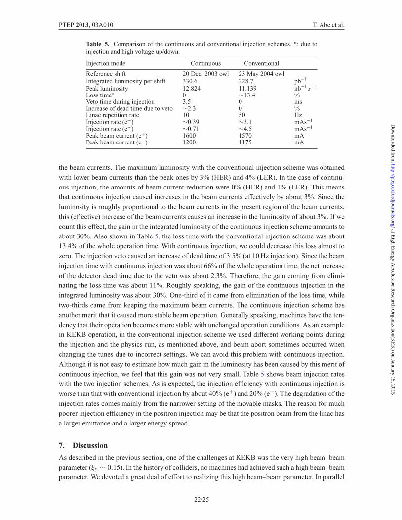
Table 5. Comparison of the continuous and conventional injection schemes. *: due toinjection and high voltage up/down.

Injection mode Continuous Conventional

Reference shift 20 Dec. 2003 owl 23 May 2004 owlIntegrated luminosity per shift 330.6 228.7 pb−1

Peak luminosity 12.824 11.139 nb−1 s−1

Loss time∗ 0 ∼13.4 %Veto time during injection 3.5 0 msIncrease of dead time due to veto ∼2.3 0 %Linac repetition rate 10 50 HzInjection rate (e+) ∼0.39 ∼3.1 mAs−1

Injection rate (e−) ∼0.71 ∼4.5 mAs−1

Peak beam current (e+) 1600 1570 mAPeak beam current (e−) 1200 1175 mA

the beam currents. The maximum luminosity with the conventional injection scheme was obtainedwith lower beam currents than the peak ones by 3% (HER) and 4% (LER). In the case of continu-ous injection, the amounts of beam current reduction were 0% (HER) and 1% (LER). This meansthat continuous injection caused increases in the beam currents effectively by about 3%. Since theluminosity is roughly proportional to the beam currents in the present region of the beam currents,this (effective) increase of the beam currents causes an increase in the luminosity of about 3%. If wecount this effect, the gain in the integrated luminosity of the continuous injection scheme amounts toabout 30%. Also shown in Table 5, the loss time with the conventional injection scheme was about13.4% of the whole operation time. With continuous injection, we could decrease this loss almost tozero. The injection veto caused an increase of dead time of 3.5% (at 10 Hz injection). Since the beaminjection time with continuous injection was about 66% of the whole operation time, the net increaseof the detector dead time due to the veto was about 2.3%. Therefore, the gain coming from elimi-nating the loss time was about 11%. Roughly speaking, the gain of the continuous injection in theintegrated luminosity was about 30%. One-third of it came from elimination of the loss time, whiletwo-thirds came from keeping the maximum beam currents. The continuous injection scheme hasanother merit that it caused more stable beam operation. Generally speaking, machines have the ten-dency that their operation becomes more stable with unchanged operation conditions. As an examplein KEKB operation, in the conventional injection scheme we used different working points duringthe injection and the physics run, as mentioned above, and beam abort sometimes occurred whenchanging the tunes due to incorrect settings. We can avoid this problem with continuous injection.Although it is not easy to estimate how much gain in the luminosity has been caused by this merit ofcontinuous injection, we feel that this gain was not very small. Table 5 shows beam injection rateswith the two injection schemes. As is expected, the injection efficiency with continuous injection isworse than that with conventional injection by about 40% (e+) and 20% (e−). The degradation of theinjection rates comes mainly from the narrower setting of the movable masks. The reason for muchpoorer injection efficiency in the positron injection may be that the positron beam from the linac hasa larger emittance and a larger energy spread.

7. Discussion

As described in the previous section, one of the challenges at KEKB was the very high beam–beamparameter (ξy ∼ 0.15). In the history of colliders, no machines had achieved such a high beam–beamparameter. We devoted a great deal of effort to realizing this high beam–beam parameter. In parallel

22/25

at High E

nergy Accelerator R


EK


Dow

nloaded from



to continuing the efforts to increase the specific luminosity at KEKB, we continued to study usingthe beam–beam simulation. We checked the validity of the beam–beam simulation code itself bycomparing two different codes. In the KEKB operation, we relied on the beam–beam simulationsdone by K. Ohmi and the introduction of the crab cavities was decided based on these simulations[12–14]. We confirmed that a different beam–beam simulation code from that by K. Ohmi gives thesame high beam–beam parameter with a horizontal tune close to the half-integer [23].

In the beam–beam simulation, only the linear lattice and the beam–beam interaction are included.Other effects, such as machine errors, lattice nonlinearity, or off-momentum optics, have been inves-tigated by adding them intentionally to the simulation code. The simulation showed that the residualx–y coupling at the IP due to machine errors would degrade the luminosity. However, as is describedin the previous section, the amount of x–y coupling at the IP that explains the discrepancy betweenthe luminosity by the simulation and that achieved in KEKB is rather large compared with thatexpected with reasonable machine errors. As for the nonlinearity of the lattice, the IR nonlinearityis dominant over the other lattice nonlinearities in high luminosity colliders with very small IP betafunctions. The IR nonlinearity was implemented in the beam–beam simulation. However, the lumi-nosity degradation due to the IR nonlinearity was negligible. The harmful effect of the chromaticityof the x–y coupling at the IP was shown by the simulation as described in the previous section. Bycorrecting these values using the skew-sextupole magnets, the luminosity increased by about 15%.The introduction of the skew-sextupole magnets was motivated by the beam–beam simulation. Anattempt to measure the chromaticity of the x–y coupling at the IP was made [24]. The results ofthe measurements showed that the chromaticity of the x–y coupling seemed to be well correctedby the skew-sextupole magnets. Although the accuracy of the measurements of the x–y couplingparameters is not good concerning their absolute values, their momentum dependence seemed tobe measured with enough accuracy. Another attempt was to implement the longitudinal wakefieldinto the beam–beam simulation [23]. The longitudinal particle distributions of both beams at KEKBgreatly deviated from a Gaussian distribution due to the potential well distortion and the microwaveinstability in the LER. However, such simulations showed that the wakefield does not have a bigeffect on the luminosity performance.

The beam–beam simulations mentioned above are based on the strong–strong model. To study theeffects of the nonlinearity of the entire lattice, a weak–strong beam–beam simulation was done usingthe SAD lattice [25]. The luminosity was consistent with the strong–strong simulation. We foundthat the linear IP coupling correction is essentially important even in the simulations considering thenonlinear lattice, as shown in Fig. 1 in Ref. [25]. Therefore, the lattice nonlinearity seems not to beimportant for luminosity performance. Another thing that we tried was to implement the crab cavitiesexplicitly into the beam–beam simulation. Note that the simulations mentioned so far do not considercrab crossing explicitly but the head-on collision was used as crab crossing. Figure 2 in Ref. [25]shows the results of the strong–weak beam–beam simulation with the SAD lattice including a singlecrab cavity. The luminosity degraded by about 25% compared with the case of head-on collisionwithout the crab cavity, even with the IP coupling correction. In KEKB, a single crab cavity per ringwas used and each bunch circulates around the ring with horizontal tilting. The tilt motion may pickup the nonlinear force along the ring (M. Zobov, private communications). Then, we carried out abeam–beam simulation where two crab cavities are located on both sides of the IP and the crabbingmotion is localized near the IP. We found that the luminosity was the same as that in the single cavitycase. We have not yet understood the mechanism of the luminosity degradation, although effects ofthe chromatic phases between the crab cavities and the IP are suspected. The effects of the crabbing

23/25

at High E

nergy Accelerator R


EK


Dow

nloaded from



motion explain some part of the discrepancy between the achievable luminosity in the strong–strongbeam–beam simulation and that in the experiment. However, there still remains a big discrepancy.

8. Conclusion

After the beam commissioning of the first four years, which has been described in a previous paper[2], the KEKB performance improved drastically and KEKB recorded the world’s highest luminosityin both the peak and integrated values. The suppression of the effects of electron clouds by thesolenoid windings in the LER was essentially important. However, at a higher LER beam currentthan about 1.6 A, the KEKB luminosity was still affected by the effects of electron clouds even withthe solenoid windings.

The luminosity tuning done by using the tuning knobs for the x–y coupling parameters and thedispersions at the IP and others was also very important for increasing the luminosity, althoughthe tuning was a very time-consuming task. Of course, the increase in the beam currents was alsoimportant for the luminosity [3].

The crab cavities worked very well until the end of the KEKB operation and imposed almost nobeam current limitation on the operation. We found that the specific luminosity with the crab cavitiesis about 20% higher than that without the crab cavities. This improvement in the luminosity is largerthan the recovery of the geometrical loss in the luminosity due to a crossing angle of about 11%. Thebeam–beam parameter, ξy , with the crab cavities reached 0.09. Although this value is very high, itis still much lower than the prediction of ξy ∼ 0.15 from the beam–beam simulation. Although theeffects of the crabbing motion explain some of the discrepancy, there still remains a big discrepancy.We could not identify the reason for this discrepancy during the period of KEKB operation. This isan unsolved problem at KEKB.

As for the efficiency in accumulating the luminosity, the realization of the continuous injectionscheme has been very important at KEKB. The gain of this scheme to the integrated luminosity wasabout 30%.

Acknowledgements

The authors would like to give their thanks to Prof. F. Takasaki and Prof. M. Yamauchi for their continu-ous encouragement throughout this work. They are also grateful to the accelerator operators from MitsubishiElectric System & Service Engineering Co., Ltd.

References[1] KEKB B-Factory Design Report, KEK-Report 95-7 (1995).[2] K. Akai et al., Nucl. Instrum. Methods Phys. Res., Sect. A 499, 191 (2003).[3] T. Abe et al., “Achievements of KEKB”, to be published in Prog. Theor. Exp. Phys.[4] K. Kanazawa et al., “Experience of KEK B-factory Vacuum System”, to be published in Prog. Theor.

Exp. Phys.[5] E. Ezura et al., “Performance and Operational Results of the RF Systems for the KEK B-Factory”, to be

published in Prog. Theor. Exp. Phys.[6] M. Akemoto et al., “The KEKB injector linac”, to be published in Prog. Theor. Exp. Phys.[7] K. Ohmi and F. Zimmermann, Phys. Rev. Lett. 85, 3821 (2000).[8] J. W. Flanagan, K. Ohmi, H. Fukuma, S. Hiramatsu, M. Tobiyama, and E. Perevedentsev, Phys. Rev.

Lett. 94, 054801 (2005).[9] H. Koiso, A. Morita, Y. Ohnishi, K. Oide, and K. Satoh, “Lattice of the KEKB Colliding Rings”, to be

published in Prog. Theor. Exp. Phys.[10] R. B. Palmer, SLAC PUB-4707 (1988).[11] K. Oide and K. Yokoya, Phys. Rev. A 40, 315 (1989).

24/25

at High E

nergy Accelerator R


EK


Dow

nloaded from

http://dx.doi.org/10.1016/S0168-9002(02)01788-6

http://dx.doi.org/10.1103/PhysRevLett.85.3821


http://dx.doi.org/10.1103/PhysRevA.40.315



[12] K. Ohmi, M. Tawada, Y. Cai, S. Kamada, K. Oide, and J. Qiang, Phys. Rev. ST Accel. Beams7, 104401 (2004).

[13] K. Ohmi, M. Tawada, Y. Cai, S. Kamada, K. Oide, and J. Qiang, Phys. Rev. Lett. 92, 214801 (2004).[14] K. Ohmi and K. Oide, Proc. EPAC’06, p. 616 (2006).[15] M. Arinaga, J. W. Flanagan, H. Fukuma, T. Furuya , S. Hiramatsu, H. Ikeda, H. Ishii, E. Kikutani, T.

Mitsuhashi, K. Mori, M. Tejima, and M. Tobiyama, “Progress in KEKB Beam InstrumentationSystems”, to be published in Prog. Theor. Exp. Phys.

[16] M. Masuzawa, Y. Funakoshi, T. Nakamura, and J. Odagiri, Proc. EPAC’06, p. 613 (2006).[17] Y. Funakoshi, M. Masuzawa, K. Oide, J. Flanagan, M. Tawada, T. Ieiri, M. Tejima, M. Tobiyama, K.

Ohmi, and H. Koiso, Phys. Rev. ST Accel. Beams 10, 101001 (2007).[18] Y. Funakoshi et al., Proc. EPAC’08, p. 1893 (2008).[19] K. Oide and H. Koiso, Phys. Rev. E 49, 4474 (1994).[20] D. Zhou, K. Ohmi, Y. Seimiya, Y. Ohnishi, A. Morita, and H. Koiso, Phys. Rev. ST Accel. Beams

13, 021001 (2010).[21] Y. Seimiya, K. Ohmi, D. Zhou, J. W. Flanagan, and Y. Ohnishi, Prog. Theor. Phys. 127, 1099 (2012).[22] K. Ohmi, R. Tomas, Y. Funakoshi, R. Calaga, T. Ieiri, Y. Morita, K. Nakanishi, K. Oide, Y. Ohnishi, Y.

Sun, M. Tobiyama, and F. Zimmerman, Phys. Rev. ST Accel. Beams 14, 111003 (2011).[23] Y. Cai, J. Flanagan, H. Fukuma, Y. Funakoshi, T. Ieiri, K. Ohmi, K. OIde, Y. Suetsugu, and J. Rorie,

Phys. Rev. ST Accel. Beams 12, 061002 (2009).[24] Y. Ohnishi, K. Ohmi, H. Koiso, M. Masuzawa, A. Morita, K. Mori, K. Oide, Y. Seimiya, and D. Zhou,

Phys. Rev. ST Accel. Beams 12, 091002 (2009).[25] K. Ohmi, J. Flanagan, Y. Funakoshi, N. Iida, H. Koiso, A. Morita, Y. Ohnishi, K. Oide, and Y. Seimiya,

Proc. EPAC’08, p. 2596 (2008).

25/25

at High E

nergy Accelerator R


EK


Dow

nloaded from

http://dx.doi.org/10.1103/PhysRevSTAB.7.104401



http://dx.doi.org/10.1103/PhysRevE.49.4474


http://dx.doi.org/10.1143/PTP.127.1099





kekb accelerator commissioning of kekbptep 2013, 03a010 t. abe et al. table 1. machine parameters...

Documents