Multi-H∞ Controller Design and Illustration on an Overhead Crane

Keivan Zavari, Goele Pipeleers and Jan Swevers

Abstract— While reliable and efficient tools are widely avail-able to solve (full-order) H∞ control problems, formulatingappropriate weighting functions constitutes the main obstacle toa good H∞ controller design. In order to facilitate the weightingfunction design, we propose to break apart the classical H∞objective into various H∞ design objectives and constraints,each relating to a particular closed-loop subsystem. The resultis a versatile and intuitive control design approach, and theresulting control problem is solved using the Lyapunov shapingparadigm. The potential of our approach is demonstrated onan overhead crane setup.

I. INTRODUCTION

The H∞ control problem concerns the design of a sta-bilizing controller K that minimizes the H∞ norm of theclosed-loop system H:

minimizeK∈S

ν (1a)

subj. to ‖H‖∞ < ν , (1b)

where S denotes the set of internally stabilizing controllers.By the end of the 90’s this problem was solved from atheoretical and mathematical viewpoint, at least for full-order controllers. Two alternative solution strategies, i.e. onebased on Ricatti equations [1] and one based on linearmatrix inequalities [2], [3], were developed and translatedinto reliable software, such as the function hinfsyn of theMatlabr Robust Control ToolboxTM. In spite of its theoreti-cal maturity,H∞ control is generally not acknowledged as aneasy and intuitive control design strategy. This is primarilydue to the fact that a closed-loop H∞ norm an sich haslimited practical value and invokes the addition of weightingfunctions. Designing appropriate weighing functions is oftenan iterative and cumbersome process, where the laboriousiterations in this design primarily follow from the fact thatall the control objectives and constraints, generally relatingto particular closed-loop subsystems, need to be merged intoone artificial objective (1a): the H∞ norm of the overallclosed-loop system.

In order to facilitate the weighting function design, wepropose to solve the controller design as a multi-objectivecontrol problem comprising multiple H∞ norms on closed-loop subsystems. This results in a more intuitive controlproblem formulation compared to (1) as it allows distin-guishing between design objectives and constraints, andimposing them on selected closed-loop subsystems. How-ever, contrary to (1), no exact convex reformulation of the

Keivan Zavari, Goele Pipeleers and Jan Swevers are with theDepartment of Mechanical Engineering, Katholieke UniversiteitLeuven, Celestijnenlaan 300B, B-3001 Heverlee, Belgium,keivan.zavari@mech.kuleuven.be.

proposed controller design problem currently exists. Wetherefore resort to the Lyapunov shaping paradigm [4], aconvex, yet conservative, solution strategy for general multi-objective control problems. Another solution strategy canbe using the less conservative G-shaping paradigm in [5].However, the paper’s major contribution is in formulating theproblem and showing that it simplifies the weighting functiondesign; more than in solving the problem. The numericalresults presented in Section III support the value of ourdesign strategy in spite of the conservatism introduced bythe Lyapunov shaping paradigm.

The contents of this paper is laid out as follows: Section IIdescribes the control problem formulation together with thenumerical solution strategy, while Section III numericallyand experimentally demonstrates its potential on an overheadcrane example. Section IV concludes the paper.Notation The set of integers is indicated by N, and Sn is theset of real symmetric n×n matrices. For a matrix X ∈ Sn,the inequalities X ≺ 0 and X � 0 mean X is negativedefinite, respectively positive definite.

II. MULTI-H∞ CONTROLLER DESIGN

Section II-A presents the control problem formulation,while Section II-B describes the numerical solution of theresulting multi-objective control problem.

A. Problem Formulation

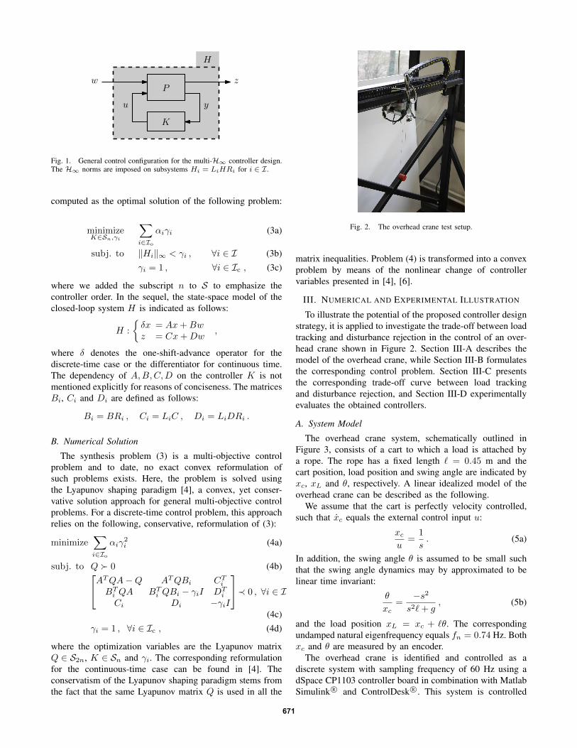
We consider a multi-objective control problem involvingvarious H∞ specifications on selected closed-loop subsys-tems. The problem is formulated in the general control con-figuration as depicted in Figure 1. The system P denotes thegeneralized plant and includes the weighting functions, K isthe controller to be designed and H denotes the closed-loopsystem. The signals u and y respectively correspond to thecontrol signal and the measured output, while the H∞ designspecifications are formulated by means of the exogenousinput w and the regulated output z. The considered H∞-norms are labelled by the index i ∈ I ⊂ N, and the ith normis imposed on closed-loop subsystem Hi of the followingform:

Hi = LiHRi , (2)

where the matrices Li, Ri select the appropriate input/outputchannels. The set I = Ic ∪ Io, where Ic groups the indicesrelating to design constraints, while Io relates to the designobjectives. The order of P is denoted by n, and only the full-order controller design is considered. That is: the controllerK is parametrized as a dynamical system of the same ordern as the generalized plant P . The controller parameters are

2012 IEEE International Conference on Control Applications (CCA)Part of 2012 IEEE Multi-Conference on Systems and ControlOctober 3-5, 2012. Dubrovnik, Croatia

978-1-4673-4504-0/12/$31.00 ©2012 IEEE 670

H

P

K

u y

zw

Fig. 1. General control configuration for the multi-H∞ controller design.The H∞ norms are imposed on subsystems Hi = LiHRi for i ∈ I.

computed as the optimal solution of the following problem:

minimizeK∈Sn,γi

∑i∈Io

αiγi (3a)

subj. to ‖Hi‖∞ < γi , ∀i ∈ I (3b)γi = 1 , ∀i ∈ Ic , (3c)

where we added the subscript n to S to emphasize thecontroller order. In the sequel, the state-space model of theclosed-loop system H is indicated as follows:

H :

{δx = Ax+Bwz = Cx+Dw

,

where δ denotes the one-shift-advance operator for thediscrete-time case or the differentiator for continuous time.The dependency of A,B,C,D on the controller K is notmentioned explicitly for reasons of conciseness. The matricesBi, Ci and Di are defined as follows:

Bi = BRi , Ci = LiC , Di = LiDRi .

B. Numerical Solution

The synthesis problem (3) is a multi-objective controlproblem and to date, no exact convex reformulation ofsuch problems exists. Here, the problem is solved usingthe Lyapunov shaping paradigm [4], a convex, yet conser-vative solution approach for general multi-objective controlproblems. For a discrete-time control problem, this approachrelies on the following, conservative, reformulation of (3):

minimize∑i∈Io

αiγ2i (4a)

subj. to Q � 0 (4b)ATQA−Q ATQBi CTiBTi QA BTi QBi − γiI DT

i

Ci Di −γiI

≺ 0 , ∀i ∈ I

(4c)γi = 1 , ∀i ∈ Ic , (4d)

where the optimization variables are the Lyapunov matrixQ ∈ S2n, K ∈ Sn and γi. The corresponding reformulationfor the continuous-time case can be found in [4]. Theconservatism of the Lyapunov shaping paradigm stems fromthe fact that the same Lyapunov matrix Q is used in all the

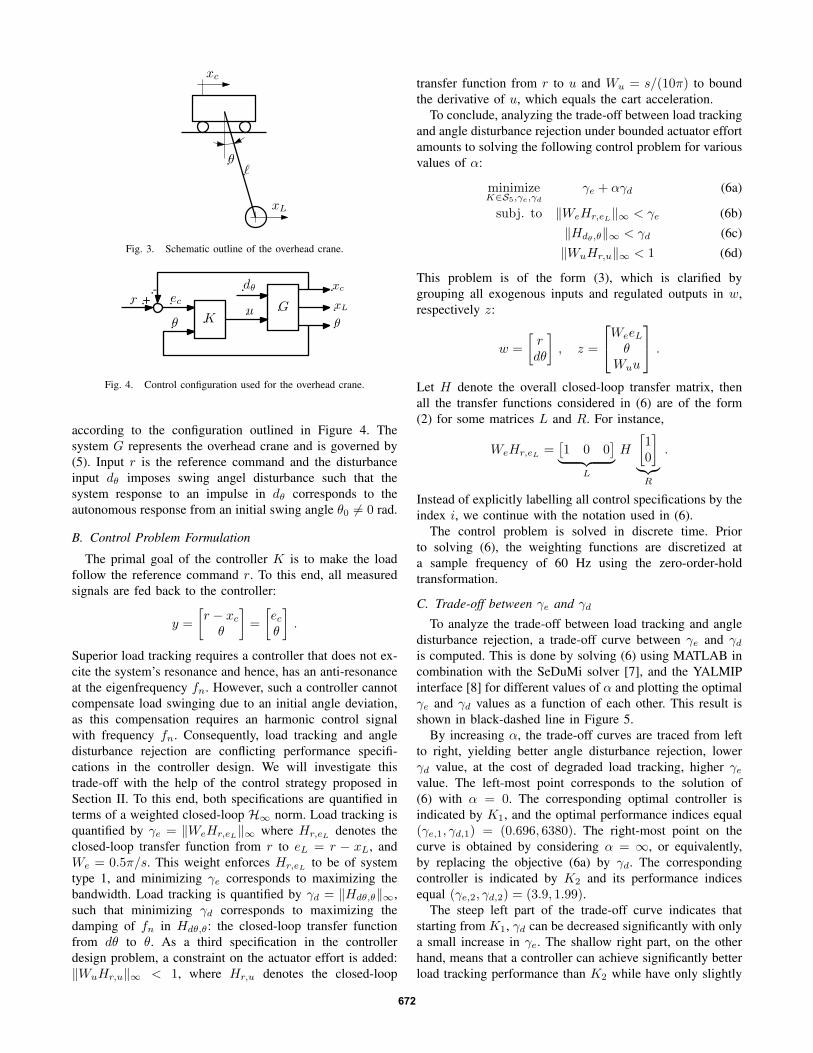
Fig. 2. The overhead crane test setup.

matrix inequalities. Problem (4) is transformed into a convexproblem by means of the nonlinear change of controllervariables presented in [4], [6].

III. NUMERICAL AND EXPERIMENTAL ILLUSTRATION

To illustrate the potential of the proposed controller designstrategy, it is applied to investigate the trade-off between loadtracking and disturbance rejection in the control of an over-head crane shown in Figure 2. Section III-A describes themodel of the overhead crane, while Section III-B formulatesthe corresponding control problem. Section III-C presentsthe corresponding trade-off curve between load trackingand disturbance rejection, and Section III-D experimentallyevaluates the obtained controllers.

A. System Model

The overhead crane system, schematically outlined inFigure 3, consists of a cart to which a load is attached bya rope. The rope has a fixed length ` = 0.45 m and thecart position, load position and swing angle are indicated byxc, xL and θ, respectively. A linear idealized model of theoverhead crane can be described as the following.

We assume that the cart is perfectly velocity controlled,such that xc equals the external control input u:

xcu

=1

s. (5a)

In addition, the swing angle θ is assumed to be small suchthat the swing angle dynamics may by approximated to belinear time invariant:

θ

xc=−s2

s2`+ g, (5b)

and the load position xL = xc + `θ. The correspondingundamped natural eigenfrequency equals fn = 0.74 Hz. Bothxc and θ are measured by an encoder.

The overhead crane is identified and controlled as adiscrete system with sampling frequency of 60 Hz using adSpace CP1103 controller board in combination with MatlabSimulink R© and ControlDesk R©. This system is controlled

671

xc

xL

θ`

Fig. 3. Schematic outline of the overhead crane.

+-

ec

θ K

dθ

u G

xc

xL

θ

r

Fig. 4. Control configuration used for the overhead crane.

according to the configuration outlined in Figure 4. Thesystem G represents the overhead crane and is governed by(5). Input r is the reference command and the disturbanceinput dθ imposes swing angel disturbance such that thesystem response to an impulse in dθ corresponds to theautonomous response from an initial swing angle θ0 6= 0 rad.

B. Control Problem Formulation

The primal goal of the controller K is to make the loadfollow the reference command r. To this end, all measuredsignals are fed back to the controller:

y =

[r − xcθ

]=

[ecθ

].

Superior load tracking requires a controller that does not ex-cite the system’s resonance and hence, has an anti-resonanceat the eigenfrequency fn. However, such a controller cannotcompensate load swinging due to an initial angle deviation,as this compensation requires an harmonic control signalwith frequency fn. Consequently, load tracking and angledisturbance rejection are conflicting performance specifi-cations in the controller design. We will investigate thistrade-off with the help of the control strategy proposed inSection II. To this end, both specifications are quantified interms of a weighted closed-loop H∞ norm. Load tracking isquantified by γe = ‖WeHr,eL‖∞ where Hr,eL denotes theclosed-loop transfer function from r to eL = r − xL, andWe = 0.5π/s. This weight enforces Hr,eL to be of systemtype 1, and minimizing γe corresponds to maximizing thebandwidth. Load tracking is quantified by γd = ‖Hdθ,θ‖∞,such that minimizing γd corresponds to maximizing thedamping of fn in Hdθ,θ: the closed-loop transfer functionfrom dθ to θ. As a third specification in the controllerdesign problem, a constraint on the actuator effort is added:‖WuHr,u‖∞ < 1, where Hr,u denotes the closed-loop

transfer function from r to u and Wu = s/(10π) to boundthe derivative of u, which equals the cart acceleration.

To conclude, analyzing the trade-off between load trackingand angle disturbance rejection under bounded actuator effortamounts to solving the following control problem for variousvalues of α:

minimizeK∈S5,γe,γd

γe + αγd (6a)

subj. to ‖WeHr,eL‖∞ < γe (6b)‖Hdθ,θ‖∞ < γd (6c)‖WuHr,u‖∞ < 1 (6d)

This problem is of the form (3), which is clarified bygrouping all exogenous inputs and regulated outputs in w,respectively z:

w =

[rdθ

], z =

WeeLθ

Wuu

.Let H denote the overall closed-loop transfer matrix, thenall the transfer functions considered in (6) are of the form(2) for some matrices L and R. For instance,

WeHr,eL =[1 0 0

]︸ ︷︷ ︸L

H

[10

]︸︷︷︸R

.

Instead of explicitly labelling all control specifications by theindex i, we continue with the notation used in (6).

The control problem is solved in discrete time. Priorto solving (6), the weighting functions are discretized ata sample frequency of 60 Hz using the zero-order-holdtransformation.

C. Trade-off between γe and γdTo analyze the trade-off between load tracking and angle

disturbance rejection, a trade-off curve between γe and γdis computed. This is done by solving (6) using MATLAB incombination with the SeDuMi solver [7], and the YALMIPinterface [8] for different values of α and plotting the optimalγe and γd values as a function of each other. This result isshown in black-dashed line in Figure 5.

By increasing α, the trade-off curves are traced from leftto right, yielding better angle disturbance rejection, lowerγd value, at the cost of degraded load tracking, higher γevalue. The left-most point corresponds to the solution of(6) with α = 0. The corresponding optimal controller isindicated by K1, and the optimal performance indices equal(γe,1, γd,1) = (0.696, 6380). The right-most point on thecurve is obtained by considering α = ∞, or equivalently,by replacing the objective (6a) by γd. The correspondingcontroller is indicated by K2 and its performance indicesequal (γe,2, γd,2) = (3.9, 1.99).

The steep left part of the trade-off curve indicates thatstarting from K1, γd can be decreased significantly with onlya small increase in γe. The shallow right part, on the otherhand, means that a controller can achieve significantly betterload tracking performance than K2 while have only slightly

672

0.6 0.8 1 1.2 1.4 1.6 1.8 20

1

2

3

4

5

γe

γd

γ trade-off in the optimization problem

actual valueoptimal value

Fig. 5. Trade-off curves of tracking performance and disturbance rejec-tion. The circled-blue point is the trade-off point which provides a goodcompromise between conflicting performances result.

TABLE ICOST FUNCTIONS OF THE MIXED-SENSITIVITY CONTROL PROBLEM.

optimal γ actual γHr,e 1.083 1.083Hr,u 1 0.7525Hdθ,θ 2.81 1.497

worse angle disturbance rejection. A good engineering choicewould therefore be a controller that corresponds to a point onthe trade-off curve with a moderate slope part, as for instanceK3, which is indicated by the blue circle in Figure 5.

To analyze the conservatism caused by the Lyapunov shap-ing paradigm used to solve the optimal control problem, thegrey dashed-dotted line in Figure 5 shows the true values ofγe = ‖WeHr,eL‖∞ and γd = ‖WθHdθ,θ‖∞ achieved by theoptimized controllers. Due to the conservatism, the optimizedγe, γd values, obtained by solving (6) according to (4),provide only an upper bound to the true performance indicesachieved by the optimized controller. Hence, in Figure 5 theblack dashed line, indicating the optimized γ values, liesabove the gray dashed-dotted line, indicating the actual γvalues, and the distance between the curves is a measure forthe conservatism of the Lyapunov shaping paradigm. Table Icompares the optimized and actual γ values for controllerK3, and confirms that the optimized γ values provide onlyan upper bound to the actual closed-loop H∞ norms.

D. Comparison of three controllers

In order to support the findings of the previous section, thecontrollers K1, K2 and K3 are further compared and imple-mented on the overhead crane shown in Figure 2. Figure 6compares closed-loop frequency response functions (FRFs)of Hr,eL , Hr,u and Hdθ,θ, while Figures 7 and 8 show theirtime-domain responses. Figure 7 shows the response to astep input of 10 cm in r and Figure 8 depicts an initial angeldeviation of the load on the experimental test setup. By the

construction of dθ, the impulse responses from dθ correspondto the autonomous responses from an initial swing angledeviation and in practice this is performed by manuallyapplying an impulse disturbance to the load. Because it isnot possible to manually apply the same disturbance to theangel at different experiments, the amplitudes are not thesame value in Figure 8. In this case the shape of the responseand settling time matter more.

The results for K1, which yields the best load tracking, areshown in dashed-red. The dashed-dotted green lines corre-spond to K2, which yields the best disturbance rejection,while the solid blue lines relate to K3, which yields agood trade-off between load tracking and angle disturbancerejection.

Figure 6 confirms that K1 yields the highest bandwidth forHr,eL . To achieve this superior load tracking performanceK1 must not excite the system’s resonance, due to which itcannot counteract the swinging initiated by an initial angledeviation. Consequently, in the FRF of Hdθ,θ the system’sundamped resonance at fn = 0.74 Hz prevails. Figures 7 and8 confirm the superior load tracking and poor disturbancerejection performance of K1.

The controller K2 yields superior disturbance rejectionat the cost of very poor load tracking, is confirmed byFrequency- and time-domain responses. Controller K3, onthe other hand, yields a good compromise between the twoperformance aspects. Compared to K1 it yields a slightlylower bandwidth in Hr,eL , while providing much moredamping to the resonance in Hdθ,θ. Compared to K2, K3

gives a slightly higher ‖Hdθ,θ‖∞, while providing a signifi-cantly higher bandwidth in Hr,eL . Figures 7 and 8 supportthese findings.

IV. CONCLUSION

This paper proposes to break apart the classical H∞control problem into H∞ objectives and constraints on se-lected closed-loop subsystems. This results in a versatile andintuitive control design approach and facilitates the weightingfunction design for the various H∞ specifications. Theresulting multi-objective control problem is solved using theLyapunov shaping paradigm. To illustrate proposed designapproach it is applied to an overhead crane example toanalyze the trade-off between angle disturbance rejection andload tracking. These results reveal the value of our approachdespite its conservatism.

V. ACKNOWLEDGEMENT

Goele Pipeleers is a Postdoctoral Fellow of the ResearchFoundation Flanders (FWO Vlaanderen). This work benefitsfrom K.U.Leuven BOF PFV/10/002 Center-of-ExcellenceOptimization in Engineering (OPTEC), the Belgian Pro-gramme on Interuniversity Attraction Poles, initiated by theBelgian Federal Science Policy Office (DYSCO), researchprojects G.0377.09 and G.0002.11 of the Research Foun-dation Flanders (FWO Vlaanderen), FP7- EMBOCON(ICT-248940), and K.U.Leuvens Concerted Research Action

673

10−2 10−1 100 101 102−100

−50

0

|Hr,u|(

dB)

10−2 10−1 100 101 102

−40

−20

0

20

|Hr,eL|(

dB)

Bode diagram of closed-loop functions

10−2 10−1 100 101 102

−200

20

40

60

frequency (Hz)

|Hdθ,θ|(

dB)

Fig. 6. Closed-loop Bode diagrams using the controller K1 (dashed-red),K2 (dash-dotted-green) and K3 (solid-blue).

0 1 2 3 4 5 6 70

0.5

1

xL

(m)

Closed-loop step response from reference input r

0 1 2 3 4 5 6 7

−0.2

−0.1

0

0.1

Time (Sec)

u(v

)

Control signal

Fig. 7. Closed-loop reference step response (top figure) and correspondingcontrol signal (bottom figure) using controller K1 (dashed-red), K2 (dash-dotted-green) and K3 (solid-blue).

0 1 2 3 4 5 6 7

−0.2

0

0.2

0.4

θ(r

ad)

Swing angle disturbance response

0 1 2 3 4 5 6 7−0.2

0

0.2

0.4

Time (Sec)

u(v

)

Control signal

Fig. 8. Swing angle disturbance response (top figure) and correspondingcontrol signal (bottom figure) using controller K1 (dashed-red), K2 (dash-dotted-green) and K3 (solid-blue).

GOA/10/11 Global real-time optimal control of autonomousrobots and mechatronic systems.

REFERENCES

[1] K. Glover and J. C. Doyle. State-space formulae for all stabilizingcontrollers that satisfy an H∞-norm bound and relations to risksensitivity. Systems & Control Problems, 11:167–172, 1988.

[2] T. Iwasaki and R. E. Skelton. All controllers for the general H∞control problem: LMI existence conditions and state space formulas.Automatica, 30(8):1307–1317, 1994.

[3] P. Gahinet and P. Apkarian. A linear matrix inequality approach toH∞ control. International Journal of Robust and Nonlinear Control,4:421–448, 1994.

[4] C. Scherer, P. Gahinet, and M. Chilali. Multiobjective output-feedbackcontrol via LMI optimization. IEEE Transactions on Automatic Control,42(7):896–911, 1997.

[5] M. C. de Oliveira, J. C. Geromel, and J. Bernussou. Extended H2

and H∞ norm characterizations and controller parametrizations fordiscrete-time systems. Int. J. Control, 75(9):666–679, 2002.

[6] I. Masubuchi, A. Ohara, and N. Suda. A linear matrix inequalityapproach to H∞ control. LMI-based controller synthesis: A unifiedformulation and solution, 8(8):669–686, 1998.

[7] J. F. Sturm, “Using SeDuMi 1.02, a Matlab toolbox for optimizationover symmetric cones,” Optimization Methods and Software, vol. 11,pp. 625–653, 1999.

[8] J. Lofberg, “Yalmip : A toolbox for modeling and optimizationin MATLAB,” in Proceedings of the CACSD Conference, Taipei,Taiwan, 2004. [Online]. Available: http://users.isy.liu.se/johanl/yalmip

674